TripleSurv: Triplet Time-adaptive Coordinate Loss for Survival Analysis

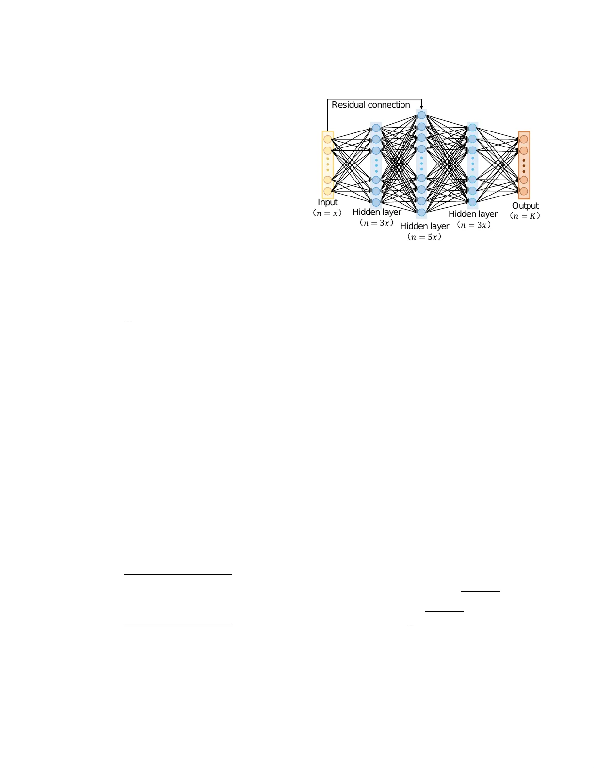
T ripleSurv: T riplet Time-adapti ve Coordinate Loss f or Surviv al Analysis Liwen Zhang, 1 * Lianzhen Zhong, 1,2 * F an Y ang, 1 Di Dong, 1 Hui Hui, 1 Jie Tian 1,3 † 1 CAS Ke y Laboratory of Molecular Imaging, Institute of Automation, Beijing, China 2 China Mobile (Hangzhou) Information T echnology Co. L TD., Hangzhou, China 3 School of Engineering Medicine & School of Biological Science and Medical Engineering, Beihang Univ ersity zhangliwen2018, zhonglianzhen2018, yangfan2022, HuiHui@ia.ac.cn, jie.tian@ia.ac.cn Abstract A core challenge in surviv al analysis is to model the distrib u- tion of censored time-to-event data, where the ev ent of inter- est may be a death, failure, or occurrence of a specific ev ent. Previous studies hav e sho wed that ranking and maximum likelihood estimation (MLE) loss functions are widely-used for surviv al analysis. Ho wev er , ranking loss only focus on the ranking of surviv al time and does not consider potential ef- fect of samples’ exact surviv al time values. Furthermore, the MLE is unbounded and easily subject to outliers (e.g., cen- sored data), which may cause poor performance of modeling. T o handle the complexities of learning process and exploit valuable survi v al time values, we propose a time-adaptiv e co- ordinate loss function, T ripleSurv , to achie ve adapti ve adjust- ments by introducing the differences in the surviv al time be- tween sample pairs into the ranking, which can encourage the model to quantitativ ely rank relativ e risk of pairs, ulti- mately enhancing the accuracy of predictions. Most impor- tantly , the T ripleSurv is proficient in quantifying the relative risk between samples by ranking ordering of pairs, and con- sider the time interval as a trade-off to calibrate the robust- ness of model over sample distribution. Our T ripleSurv is ev aluated on three real-world survi val datasets and a public synthetic dataset. The results show that our method outper- forms the state-of-the-art methods and exhibits good model performance and robustness on modeling various sophisti- cated data distributions with differe nt censor rates. Our code will be av ailable upon acceptance. 1. Introduction Surviv al analysis is a set of techniques to analyze data re- lated to the duration of time until an ev ent of interest occurs (Jing et al. 2019). This approach is applied in se v eral fields including medicine, engineering, economics, and sociology . The purpose of surviv al analysis is to assess the impact of certain v ariables on surviv al time (Bello et al. 2019). As an example, a surviv al analysis can be used to in vestigate the relationship between clinical factors (e.g., age, gender, and race) and heart attack risk. Additionally , survi v al analysis is frequently utilized in the medical field to identify which * These authors contributed equally . † Corrsponding author . Copyright © 2023, Association for the Adv ancement of Artificial Intelligence (www .aaai.org). All rights reserved. factors have the greatest impact on disease recurrence (Jing et al. 2019). Standard statistical and machine learning methods are widely used for surviv al analysis. Cox Proportional Haz- ards (CPH) (Cox 1972) is one of prev alent models, which calculates the effects of variables on the risk of an ev ent happening. The CPH model is based on the assumption that patients’ risk of death is a linear combination of their v ari- ables. Howe ver , this assumption is too strong to reflect the real-world nonlinear relationships between survi v al time and variables. Recently , researchers ha ve attempted to impro ve the performance of surviv al analysis models by incorporat- ing deep learning techniques to augment the con ventional Cox model (Katzman et al. 2018). Previous study introduce a deep generati ve model within the framew ork of parametric censored regression (Ranganath et al. 2016). Howe v er , these deep surviv al analysis models still possess strong assump- tions of the CPH model. T o address the limitations of pre vious deep surviv al anal- ysis models, discrete-time survi v al analysis based on Max- imum Likelihood Estimation (MLE) draws much attention (Lee et al. 2018). This approach segments the observation period into multiple time interv als, and then predicts survi val time by determining if the event of interest has occurred at certain interval. For instance, a deep neural network (DNN) was proposed in (Lee et al. 2018) that combines ranking loss and likelihood loss to predict the probability density v alues for discrete-time surviv al analysis. Additionally , techniques such as multi-task learning algorithm (Li et al. 2016) and re- current neural networks (RNN) (Ren et al. 2019), the studies hav e been used to capture the relationships between adjacent time intervals. The loss function is a crucial component of survi v al model learning. Some studies hav e optimized survi v al models us- ing ranking loss by predicting the order of surviv al times in pairs of samples (Lee et al. 2018). Howe ver , the original ranking loss function only focuses on the order of predicted values rather than the specific values themselves, and disre- garding the quantitative dif ferences of surviv al time for in- dividuals. Besides, some researchers currently focus on the calibration performance of survi v al model (Goldstein et al. 2020). Calibration refers to that predictions are consistent with observations, a well-calibrated surviv al model is one where the predicted probabilities ov er e v ents within any time interval are consistent with the observ ed frequencies of their occurrence (A vati et al. 2020). Although these methods do not make any strong assumptions about the underlying dis- tribution of survi val time or survi val function, they still have some limitation: 1) Not consider potential effect of samples’ exact surviv al time v alues; 2) improving the model perfor - mance from a single aspect, without re vealing the relation- ship between accuracy and rob ustness of models. T o address these issues, we propose a novel loss function, T ripleSurv , to further optimize the modeling process from dif ferent per - spectiv es. Main contributions of our w ork are summarized as follows: • W e propose a time-adapti ve pairwise loss function to ex- ploit v aluable survi v al information, and achie ve adapti v e adjustments by introducing the dif ferences in the survi val time between sample pairs into the ranking, which can encourage the model to quantitati vely rank relativ e risk of pairs, ultimately enhancing the accuracy of predic- tions. • W e propose a coordinate loss function of T ripleSurv to optimize the modeling process. The TripleSurv strikes a balance to facilitate the model to takes into account the data distribution, ranking, and calibration. • Our T ripleSurv is e v aluated on four public datasets. The results demonstrate that our method outperforms the state-of-the-art and existing methods and achie ves good performance and robustness on modeling various sophis- ticated data distributions with the highest geometrical and clinical metrics. Most importantly , our method also performs well on datasets with large censoring rates. 2. Related work W e re vie w three streams of related work for surviv al loss function in terms of the technical components of this work: 1) Likelihood estimation; 2) Ranking; 3) Calibration. A brief summary can be found in Appendix A. 2.1. Methods Based on Lik elihood Likelihood estimation function is a commonly used to opti- mize surviv al analysis models. One of representativ e Like- lihood estimation functions is Maximum Lik elihood Esti- mation (MLE). Though MLE corresponds to a proper scor- ing rule for modeling distribution, it is sensitiv e to out- liers (Kamran and Wiens 2021). This sensiti vity may re- sult in poor generalization of model. Continuous Ranked Probability Score (CRPS) is a great substitution of MLE which has been widely used in meteorology (Gneiting and Katzfuss 2014). The CRPS gi v es more calibrated forecasts compared with MLE. More importantly , CRPS could im- porve the sharpness of probabilistic forecast which is more practical for survi v al models (Ranganath et al. 2016; A vati et al. 2018; Rajkomar et al. 2018). A vati et al. introduced a Surviv al-CRPS (S-CRPS) for survi v al analysis which e x- tended CRPS to handle right and interval-censored data. Nev ertheless, although S-CRPS shows good robustness, it does not gives a straightforward w ay to balance model per- formance between the discrimination and robustness. 2.2. Methods Based on Ranking Ranking for survi v al analysis is a statistical method used to analyze the time-to-ev ent data, where the events of interest are rank ed or ordered. The Concordance Index (C-index) is a widely used metric for ranking (Harrell et al. 1982). The C-index focuses on ranking problem which calculates a ra- tio of corrected ordered pairs among all possible comparable pairs. Howe v er , it can’t be directly used as an objectiv e func- tion during training for it is in variant to any monotone trans- formation of the surviv al times (Steck et al. 2007). T o o ver - come this problem, a number of related works have emerged considering ranking problem by introducing ranking loss in- train to improv e the ranking ability of surviv al models. Ad- ditionally , Cox’ s partial likelihood function (Cox 1975) is commonly used as the objectiv e function in Cox propor- tional hazard model (Katzman et al. 2018; T ibshirani 1997), which describes the risk of an ev ent occurring for an individ- ual at a specific time point, given certain cov ariates. Raykar et al. proved that maximizing this likelihood also ends up ap- proximately maximizing the C-index. Recently , many works attempt to improv e C-index by combining ranking loss func- tion in-training (Lee et al. 2018; W ang, Li, and Chignell 2021; Jing et al. 2019). The study (Lee et al. 2018) pro- posed a deep learning method for modeling the ev ent prob- ability without assumptions of the probability distribution by combining MLE with a ranking loss. In RankDeepSurv (Jing et al. 2019), the authors combine a selecti v e ranking loss with MSE. Howe v er , these work mainly focus on or- dering relationship between comparable pairs b ut ignore the specific numerical differences for survi val time. 2.3. Methods Based on Calibration Calibration refers to that predictions are consistent with ob- servations, a well-calibrated survi val model is one where the predicted probabilities over e vents within any time interval is consistent to the observed frequencies of their occurrence (A v ati et al. 2020). Survi v al models with poor calibration can cause poor generalization for predicting the distrib ution if real-world survi v al data (Shah, Steyerber g, and K ent 2018; V an Calster and V ickers 2015). Recently , many studies deal with calibration problems in-training for surviv al model. A v ati et al. (A vati et al. 2020) replaced the common used partial lik elihood loss with Survi val-CRPS, which could im- plicitly balance between prediction and calibartion. Kamran proposed rank probability score(RPS) which is a discrete approximation based on CRPS as well. Concurrently , Gold- stein et al. proposed an explicit differentiable calibration loss of X-CAL (Goldstein et al. 2020) for boosting model ro- bustness in-training. Howe ver , X-CAL doesn’t disclose the relationship between the discrimination and robustness. 3. Methods In this section, we mainly introduce survi v al data, data pre- processing, methodology of our proposed method, and e v al- uation metrics. 3.1. Survival Data Surviv al data consist of three pieces of information (  X , t, δ, ) for each sample: 1) The vector  X denotes av ail- able co variates; 2) observed survi v al time t elapsed between enrollment time and the time of the failure or the censoring, whichev er occurred first; 3) a label indicating the status of ev ent δ (e.g. recurrence or death). One peculiar feature for surviv al data is kno wn as censoring. A censored sample sig- nifies that a patient did not experience the failure during the observed time interv al. 3.2. Data Pr eprocessing T o standardize the surviv al time, we normalize it to a range of 0 to 1. W e also define T max = max { t i | δ i = 1 } , and T min = min { t i | δ i = 1 } . Since the surviv al times of cen- sored samples may be greater than T max , and the last inter - val needs to b e left to correspond to infinity , T max corre- sponds to K-2, T min corresponds to 0. The diagram is shown as Figure 1.   0 1 K - 3 K - 2 K - 1 K ……      Figure 1: Diagram of the interval partition of study time. T o lea ve a certain interval, in fact, we make T max corre- spond to K-2.1, T min corresponds to 0.1, so the time interval of each interval ∆ T = T max − T min K − 2 . 2 , and then the study time t is normalized according to follo w formulas: cr op ( x, a, b ) = ( a, x < a b, x > b x, other , (1)            T ′ min = T min − 0 . 1 ∗ ∆ T T 1 max = T ′ min + ( K − 1) ∗ ∆ T T 2 max = T ′ min + K ∗ ∆ T t ′ = cr op ( t, T ′ min , T 1 max ) ˜ t = ( t ′ − T ′ min ) / ( T 2 max − T ′ min ) , (2) where the width corresponding to each time interv al after normalization is 1 K − 1 . The k-th interv al represents the time interval [ k − 1 K , k K ) , corresponding time t bin k = 2 k − 1 2 K . Unless otherwise specified, the study time t refers to the time after normalization in the following conte xt. 3.3. Proposed T APR-loss and T ripleSurv W e introduce our proposed loss function in two parts: 1) Theoretical description of our proposed time-adapti v e pair - wise rank loss (T APR-loss); 2) Theoretical description of our proposed integrating T ripleSurv equipped with T APR- loss. Proposed T APR-loss Our proposed time-adaptiv e pair- wise ranking loss (T APR-loss) is inspired by ranking loss (Lee et al. 2018). The ranking loss function optimizes di- rectly the pairwise orders: the longer-li v ed one among com- parable pair hav e a lo wer risk than the other: l rank = 1 | A 1 | X i ∈ A 1 X j ∈ R ( i ) Π( r isk i − r isk j ) , (3) where A 1 = { i | δ i = 1 } , R ( i ) is called the risk set and is defined as R ( i ) = { j | t j > t i } , r isk i signifies the estimated risk of the sample i , Π( · ) is the indicator function, and | · | is a counting function for a set. Since the indicator function is non-dif ferentiable, we generally use a function η ( · ) to ap- proximate the indicator function. Lee et al. (Lee et al. 2018) used η ( risk i , r isk j ) = exp ( σ ∗ ( r isk i − r isk j )) and rewrote the rank loss as follows: l rank = 1 | A 1 | X i ∈ A 1 X j ∈ R ( i ) exp ( σ ∗ ( F ( t i |  X i ) − F ( t i |  X j ))) , (4) where F ( t i |  X i ) signifies the probability of f ailure occurring at time t i and the gi v en co v ariates  X i . σ is a scalar h yperpa- rameter . The rank loss only considers the relati ve ranking of the surviv al time but ignore the important quantitative differ - ence (Lee et al. 2018; Raykar et al. 2007), resulting in count- less optimal solutions for the optimization problem, ev en in- valid forecasts. T o mitigate the issues, we extend the idea of concordance and assume that the risk difference between the comparable pair is proportional to the difference of failure times between them. According to the assumption, we add the dif ference of f ailure times into the rank loss, forming the T APR-loss: l T AP R − l oss = 1 | A 1 | X i ∈ A 1 X j ∈ R ( i ) exp ( σ ∗ [( r isk i − r isk k ) − ρ ∗ ( t j − ti )]) , (5) where we refine r isk = 1 − mean dead time = 1 − P K k − 1 p k ∗ t bin k , σ and ρ are scalar hyperparameters, σ ∈ (0 , 1] . Considering t bin k ∈ [ 1 2 K , 2 K − 1 2 K ] , we can infer 1 2 K = 1 − 2 K − 1 2 K P K k =1 p k < r isk ≤ 1 − 1 2 K P K k =1 p k = 2 K − 1 2 K , and r isk ∈ [ 1 2 K , 2 K − 1 2 K ] . T ripleSurv: strike a trade-off time-adaptive coordinate loss T o improve the performance and robustness of model and exploit valuable survial time, we propose the T ripleSurv to optimize the modeling process in multiple scale (single- sample, pairs, and population level) by integrating the lik e- lihood loss, T APR-loss, and calibration loss: l T ripleS ur v = − α ∗ l likel ihood − β ∗ l T AP R − l oss + γ ∗ l calibr ation , (6) where α , β and γ are scalar hyperparameters, which are suggested to set for ensuring that the values of these three items are at the same lev el of magnitude. Likelihood loss ( l likel ihood ) Theoretically , we need to es- timate probability density function f ( t |  X ) and the likeli- hood can be written as follows: l likel ihood =  f ( t |  X ) , δ = 1 S ( t |  X ) , δ = 0 , (7) where S ( t |  X ) is surviv al function. δ = 1 represent ev ent status is observed while δ = 0 represent ev ent status is not observed. In this study , we use the discrete probability mass function P ( t |  X ) = [ p 1 , p 2 , ..., p k ] in k disjoint time inter- vals, which is often predicted in academic research and clin- ical practical, and its definition and the likelihood can be written as follows: l likel ihood =  p k , δ = 1 1 − P k i =1 , δ = 0 , (8) where p k , k = 1 , 2 , ..., K , signifies the probability of the failure occurring in a specific time interval [ a k , b k ) , k de- notes the index of time interv al that study time t falls. Calibration loss ( l calibr ation ) W e combine the calibration loss with other objecti v es for optimization during training to strike a desired balance between discrimination and robust- ness.    l calibr ation = 1 G P G g =1 ( pr ed g − obse g ) 2 pr ed g = ( P i P t bin k ∈ I g p i k ) / ( P i P t bin k >a g p i k ) obse g = |{ i | a g ≤ t i < b g , e i = 1 }| / |{ i | a g ≤ t i }| . (9) W e compute the squared errors between the observ ed and predicted failure incidence within G time intervals. Obvi- ously , the optimization of calibration constrains the distrib u- tion of the model prediction in population level, which can play an important role of regularization in training process. 3.4. Model Description W e exploit Categorical (Cat) and Multi-T ask Logistic Re- gression (MTLR) methods (Goldstein et al. 2020) equipped with our proposed loss to model the distribution of failure occurring o ver discrete times. The Cat method is parameter- ized by using a deep neural network function of with K bins as outputs, which can approximate the continuous surviv al distribution as K → ∞ . MTLR method is similar to the Cat method except that it allows the model to produce K − 1 outputs. Assume a survi v al model with MTLR method out- puts a vector φ = [ φ 1 , φ 2 , ..., φ K − 1 ] , the estimation of the probability mass function for bin k < K is: p k = exp ( P K − 1 j = k φ j ) 1 + P K − 1 i =1 exp ( P K − 1 j = i φ j ) , (10) and the estimation of the probability mass function for bin K is: p k = 1 1 + P K − 1 i =1 exp ( P K − 1 j = i φ j ) . (11) As for one-dimensional data, we use a four layer fully- connected residual neural network (Figure 2) as the archi- tecture of the survi v al models, which is similar to the pro- posed model by Lee et al (Lee et al. 2018). F or the public synthetic dataset, we use shallow ResNet (He et al. 2016) as the architecture. The Batch Normalization is used in the architectures. Res i dual c onnec ti on I nput （ 𝑛 = 𝑥 ） H i dden l ay er （ 𝑛 = 3𝑥 ） H i dden l ay er （ 𝑛 = 5𝑥 ） H i dden l ay er （ 𝑛 = 3𝑥 ） O utput （ 𝑛 = 𝐾 ） Figure 2: The fully-connected neural network for one- dimensional data. 3.5. Evaluation Metrics W e use popular metrics of Concordance index (C-inde x), Brier Score, and T ime-dependent area under the R OC (TD A UC) for e valuation of model performance from dif- ferent aspects. Moreov er , in our study , risk stratification for real-world data is also conducted to assess the benefit of the surviv al models for selection of decision-making. W e intro- duce the definition of these metrics for easy to reproduce in Appendix B. Concordance Index (C-index) The C-index is a widely- used metric for survi v al models, which se vers as a repre- sentativ e indicator for rank relationship between predicted risk scores ˆ r and observ ed time points t . A C-inde x of 1.0 indicates perfect discrimination, while a C-index of 0.5 rep- resents no discrimination ability . Integrated Brier Score The Integrated Brier Score (IBS) is an extension of the time-dependent Brier score for surviv al model with cencored data. Time-dependent Brier score is a tailored metric is extended by Graf et al. (Graf et al. 1999) and widely-used to measures the capability of calibration. The metric uses in verse probability of censoring weights, which requires estimating the censoring survi v al function, denoted as ˆ G ( t ) over time points t . The time-dependent Brier score is defined as:        I sum i ( t ∗ ) = I ( t i ≤ t ∗ & δ i = 1) ( 0 − ˆ S ( t ∗ ) ) 2 ˆ G ( t i ) + I ( t i > t ∗ ) ( 1 − ˆ S ( t ∗ ) ) 2 ˆ G ( t ∗ ) B S ( t ∗ ) = 1 n P n i =1 I sum i ( t ∗ ) , (12) where I ( · ) represents observed ev ent status, n is number of samples, and ˆ S ( t ) is the observed rate of e vent-free samples at t ∗ . IBS can be defined given an av erage IBS across the time in intervals of T ∗ : IBS( T ∗ ) = 1 T ∗ Z T ∗ 0 B S ( t ∗ ) dt ∗ . (13) Time-dependent area under the ROC (TDA UC) The metirc of TD A UC is a performance ev aluation metric for binary classifiers that takes into account the classifier’ s performance changes over time (Kamarudin, Cox, and K olamunnage-Dona 2017). At a gi v en time point t and a cutoff c , W e define them as: T D AU C ( t, X ) = Aer a { sensitivity ( c, t ) , 1 − specif icity ( c, t ) } . (14) W e use the mean of TDA UC (mTD A UC) ov er the time to de- termine ho w well estimated risk scores can distinguish dis- eased patients from healthy patients: mT D AU C ( X ) = 1 n t X T D AU C ( t i , X ) , (15) where n t denote the number of time points. Hazard Ratio The hazard ratio (HR) is a measure of the relativ e risk of an event occurring in one group compared to another group ov er time. T o ev aluate the effecti v eness of different decision-making, decision implementation mainly is based on risk stratification with HR, where samples are divided into lo w-risk and high-risk groups by a risk factor r and are recommended a f av orable regimen. The cutof f of the risk factor is determined by the partition with the maximal log-rank test statistic in the training set. 4. Experiments and Results 4.1. Competing Methods a. Lasso-Cox The Cox proportional hazards (CPH) model is the most frequently used survi val model (Jing et al. 2019). Generally , to av oid wrong estimation caused by redundant input features, the Least Absolute Shrinkage and Selection Operator (LASSO) is used to perform feature selection be- fore building CPH model. The y are often used together . b . RSF The Random Surviv al Forests (RSF) is a popular nonlinear surviv al model that is based on the tree method and produces an ensemble estimate for the cumulative haz- ard function. c. DeepSurv DeepSurv model (Katzman et al. 2018) is a CPH model based on full connect neural network that opti- mizes the partial likelihood loss and outputs directly for the surviv al risk prediction. d. DeepRank W e formulate the DeepRank model as the comparison model that optimizes the rank loss (Lee et al. 2018). e. CRSP Survi v al-CRPS (CRPS) (A vati et al. 2020) is sharpness subject to calibration b ut it optimizes neither the calibration loss nor the traditional likelihood loss. f. X-cal X-cal model (Goldstein et al. 2020) combines the likelihood loss and explicit calibration for estimating the dis- tribution of survi v al function. g. DeepHit The DeepHit model (Lee et al. 2018), intro- duced by Lee et al. in 2018, is a deep neural network that predicts the probability p ( z ) of an e vent occurring over the entire time space given an input x . This method e xhibits state-of-the-art performance for modelling distribution of time-to-ev ent data. h. Cat integrating differ ent loss functions Cat is an ab- breviation of categorical method (Goldstein et al. 2020). This method regards surviv al analysis as a classification task, which discretizes the surviv al time of patients into sev eral time interv al bins, and then predicts the probabil- ity of each or falling in its corresponding interval bins. In our study , we compared different Cat methods integrating CRSP (Cat-crps), X-cal (Cat-xcal), DeepHit (Cat-hit), and our method (Cat-ours). i. MTLR integrating different loss functions MTLR (Li et al. 2016) method is different from the Cat method con- sidering some relationships between the probability of the time interval bins. W e also compared our method (MTLR- ours) integrating our proposed loss function with MTLR- crps, MTLR-xcal, and MTLR-hit. 4.2. Implementation Details W e use SGD optimizer and the “cosine annealing” learning schedule to update training weights. The initial learning rate is set as 1e-3 or 1e-2 where appropriate. The rate of dropout is set as 0.2 unless otherwise specified. The weight of each component in TripleSurv loss, α , β , and γ , are set to ensure the same lev el of magnitude for their v alues in the training datasets. The σ , ρ are determined according to the model performance in the validation dataset. In each experiment setting, the final model used for model e v aluation w as de- termined using its performance in terms of the C-index in the validation. The default ratio of training, v alidation, and test sets is approximately 3:1:1. For the small sample size of MET ABRIC (n=1981), we employ fiv e-fold cross-validation for performance ev aluation of dif ferent methods. More de- tails for easy reproduction in Appendix C. 4.3. Datasets and T asks SUPPOR T The Study to Understand Prognoses Prefer- ences Outcomes and Risks of Treatment (SUPPOR T) is a comprehensiv e study that assessed the survi v al time of criti- cally ill adults who were hospitalized (Jing et al. 2019). The SUPPOR T comprises 9105 patients and encompasses 14 dif- ferent features. In the dataset, the censor rate is 31.9%. T o- tally 68.10% of the dataset was observed data. BIDDING BIDDING real-time bidding dataset that con- tains auction request information, bid price, and the status whether bidders win the auction. Researchers treat the bid price as the time and whether winning of the auction as the ev ent status for surviv al analysis, and treat winning prob- ability estimation of a single auction as a task (Ren et al. 2019). MET ABRIC W e ev aluate dif ferent methods for the pre- diction of overall surviv al of patients with breast cancer from the Molecular T axonomy of Breast Cancer Interna- tional Consortium (MET ABRIC) dataset (Lee et al. 2018). T otally 1980 patients are av aliable in the dataset, which contains gene expression profiles and clinical features (Jing et al. 2019). Among all patients, 888 (44.8%) were followed until death, while the remaining 1093 (55.2%) were right- censored. MINIST Moreover , a public synthetic dataset (Goldstein et al. 2020) based on the MNIST is considered for ev aluat- ing our proposed method. The synthetic survi v al times are conditional on the MNIST classes.The settings for MNIST are the same as (Goldstein et al. 2020). More details for statistics of all datasets are summarized in Appendix D. 4.4. Results and Analysis Four experiments are conducted and sho w that our proposed T ripleSurv performs well on datasets with different cen- soring rates. Compared to existing loss functions of MLE (Ren et al. 2019), rank loss (Lee et al. 2018), and calibra- tion (Goldstein et al. 2020), our T ripleSurv achiev es the best ranking accuracy and robustness on four datasets. More de- tails for prognostic risk e v aluation can be found in Appendix E. Method C-index( ↑ ) mTD A UC( ↑ ) IBS( ↓ ) HR( ↑ ) Random(ref) 0.500 0.500 0.2520 1.00 Lasso-cox 0.725 0.754 0.1846 2.92 RSF 0.713 0.762 0.1806 2.99 DeepSurv 0.721 0.757 0.1867 3.00 DeepRank 0.723 0.742 0.1906 2.77 Cat-crps 0.675 0.684 0.1999 2.19 Cat-xcal 0.704 0.728 0.1908 2.55 Cat-hit 0.712 0.757 0.1843 3.01 Cat-ours 0.726 0.762 0.1803 3.04 MTLR-crps 0.701 0.724 0.1918 2.53 MTLR-xcal 0.701 0.744 0.1892 2.69 MTLR-hit 0.711 0.761 0.1840 3.07 MTLR-ours 0.727 0.765 0.1804 3.04 T able 1: Performance comparison in SUPPOR T . C- index:Concordance Inde x; mTD A UC: mean T ime- dependent area under the R OC; IBS: Integrated Brier Score; HR: hazard ratio (clinical metric for risk ev aluation). Experiment 1: Overall survival prediction in SUPPOR T As shown in T able 1, compared to existing deep surviv al models, the Cat-ours achieved the highest C-index, mT - D A UC (the e v aluation of TDA UC at each time point is shown in Figure 3), and the lowest IBS. The same results were also observed in MTLR-ours. The results indicate that our proposed TripleSurv has excellent discriminati ve abil- ity and can achiev e a good balance between discriminative ability and robustness for survi v al models. Experiment 2: Winning prediction at auction in BID- DING Our models (Cat-ours and MTLR-ours) ha v e the best discriminativ e and calibration capability (T able 2 and Figure 4). For surviv al models based on CRPS loss, the 0.0 0.2 0.8 1.0 0.80 0.70 0.75 0.75 Time−dependent AUC 0.4 0.6 Time from enrollment lasso_c ox rsf cat_c r ps cat_xcal cox_parl cat_hit cox_rank cat_ours 0.0 0.2 0.8 1.0 0.65 0.4 0.6 Time from enrollment Time−dependent AUC 0. 7 0 lasso_c ox rsf mtlr_crps mtlr_xcal cox_parl mtlr_hit cox_rank mtlr_ours A B 0.60 0.60 0.85 0.65 0.85 0.80 Multi-task method (mtlr) as backbone in SUPPORT Categorical method (cat) as backbone in SUPPORT Figure 3: Performance comparison using the TD A UC in SUPPOR T . Method C-index( ↑ ) mTD A UC( ↑ ) IBS( ↓ ) HR( ↑ ) Random (ref) 0.500 0.500 0.2926 1.00 Lasso-cox 0.699 0.716 0.2234 3.07 RSF 0.766 0.791 0.1945 3.66 DeepSurv 0.762 0.778 0.1990 3.65 DeepRank 0.760 0.777 0.2091 3.69 Cat-crps 0.680 0.695 0.2900 2.41 Cat-xcal 0.723 0.742 0.2009 2.92 Cat-hit 0.761 0.783 0.2061 3.52 Cat-ours 0.782 0.800 0.1922 3.95 MTLR-crps 0.751 0.767 0.2392 3.14 MTLR-xcal 0.727 0.750 0.1997 3.02 MTLR-hit 0.773 0.791 0.2078 3.59 MTLR-ours 0.785 0.801 0.1935 3.76 T able 2: Performance comparison in BIDDING results show a significant difference between Category and MTLR methods. The performance of nonlinear sur- viv al models is generally better than linear surviv al models (Lasso-cox). 0.2 0 . 1 0 . 0 0.8 0.70 cox_parl cox_parl cat_hit cox_rank cox_rank cat_ours 0.4 0.6 0.60 0.65 0.75 0.80 0.85 0.90 Time−dependent AUC Time from enrollment lasso_cox rsf rsf cat_crps cat_xcal mtlr _crps mtlr _xcal mtlr_hit mtlr _ours 0.70 0.60 0.65 0.75 0.80 0.85 0.90 Time−dependent AUC 0.2 0 . 0 0.8 0.4 0.6 Time from enrollment 0 . 1 A B lasso_cox Categorical method (cat) as backbone in BIDDING Multi-task method (mtlr) as backbone in BIDDING Figure 4: Performance comparison using the TD A UC in BIDDING. Experiment 3: Overall survi val pr ediction in MET ABRIC As is shown in T able 3, compared to other competing models, the Cat-ours achiev ed the highest C-index, mTDA UC (e valuation of TD A UC at each time point is sho wn in Figure 5), and the lowest IBS. The same results were observed in the MTLR-ours. For surviv al models based on the X-cal loss, the poor performance showed a lar ge dif ference between the Cat and MTLR method. In terms of risk stratification ability , the Cat-ours model identified 63% of patients as high-risk patients with the highest risk ratio (HR=2.70) between high and low-risk patients, while the MTLR-ours model identified 53% of patients as high-risk patients with the second highest risk ratio (HR=2.0) between high and lo w-risk patients. Other surviv al models hav e lo wer ability in identifying high-risk patients. Method C-index( ↑ ) mTD A UC( ↑ ) IBS( ↓ ) HR( ↑ ) Random (ref) 0.500 0.500 0.2500 1.00 Lasso-cox 0.654 0.647 0.1862 2.18 RSF 0.674 0.660 0.1891 2.46 DeepSurv 0.670 0.674 0.1886 2.36 DeepRank 0.675 0.680 0.1918 2.44 Cat-crps 0.659 0.648 0.1911 2.26 Cat-xcal 0.660 0.665 0.1907 2.27 Cat-hit 0.674 0.679 0.1954 2.17 Cat-ours 0.688 0.695 0.1878 2.70 MTLR-crps 0.662 0.644 0.1899 2.15 MTLR-xcal 0.612 0.614 0.1980 1.86 MTLR-hit 0.671 0.677 0.1874 2.32 MTLR-ours 0.679 0.681 0.1870 2.50 T able 3: Performance comparison in MET ABRIC 0.0 0.2 0.8 1.0 0.60 0.65 0.75 0.80 0.4 0.6 0.70 Time−dependent AUC Time from enrollment lasso_c ox rsf cat_c r ps cat_xcal cox_parl cat_hit cox_rank cat_ours 0.0 0.2 0.8 1.0 0.60 0.65 0.75 0.80 0.70 Time−dependent AUC 0.4 0.6 Time from enrollment lasso_c ox rsf mtlr_crps mtlr_xcal cox_parl mtlr _hit cox_rank mtlr _ours A B Categorical method (cat) as backbone in MET ABRIC Multi-task method (mtlr) as backbone in MET ABRIC Figure 5: Performance comparison using the TD A UC in MET ABRIC. Experiment 4: Surviv al prediction in synthetic MNIST In this experiment, The failure time of survival MNIST is synthetic but real clinical data, so we do not perform the risk stratification. The experimental results were summarized in T able 4. Our model, using either the Category method or the MTLR method, has the highest C-index and mTDA UC compared to other models (as shown in Figure 6). The MTLR-hit ha v e the better IBS than ours since our models take model rob ust- ness into consideration. Observing Figure 6 shows that sur- viv al models based on partial lik elihood and xcal combina- tion loss have significant shortcomings in predicting failure risks at early times. 4.4. Ablation Study W e conduct our ablation experiments using BIDDING dataset since it has the largest sample size among the three Method C-index( ↑ ) mTDA UC( ↑ ) IBS( ↓ ) Random (ref) 0.500 0.500 0.2500 DeepSurv 0.929 0.936 0.0658 DeepRank 0.951 0.994 0.0271 Cat-crps 0.942 0.983 0.0255 Cat-xcal 0.879 0.942 0.0591 Cat-hit 0.945 0.991 0.0061 Cat-ours 0.956 0.995 0.0060 MTLR-crps 0.948 0.991 0.0226 MTLR-xcal 0.908 0.955 0.0480 MTLR-hit 0.951 0.994 0.0051 MTLR-ours 0.956 0.995 0.0061 T able 4: Performance comparison in MNIST cox_parl cox_rank mtlr_cr ps mtlr_xcal mtlr_hit mtlr_ours cat_xcal cat_hit cat_ours cox_parl cox_rank cat_crps A B 0.0 0.2 0.8 1.0 0.80 0.85 0.95 1.00 0.4 0.6 0.90 Time−dependent AUC Time from enrollment 0.0 0.2 0.8 1.0 0.80 0.85 0.95 1.00 0.90 Time−dependent AUC 0.4 0.6 Time from enrollment Multi-task method (mtlr) as backbone in MNIST Categorical method (cat) as backbone in MNIST Figure 6: Performance comparison using the TD A UC in MNIST . real-world datasets. The experiment settings are the same as those set in mentioned experiments. The experimental results indicate that our methods exhibit superior perfor- mance (T able 5 and 6). Additionally , the model based on our T APR loss also outperformed the models based on the existing Rank loss in these three metrics. W e found that the our model(Cat-ours) had a slightly higher C-inde x (0.782 vs. 0.779) and similar mTD A UC (0.800 vs. 0.801) com- pared to the model using likelihood and T APR-loss, but a significantly higher IBS (0.1922 vs. 0.1993). The same re- sults were also found for the MTLR-ours. These results sug- gest that adding a calibration loss function to the combina- tion of likelihood and T APR losses can slightly improve the model’ s discrimination ability and its robustness. Further- more, although the model only based on MLE sho wed the highest IBS, it may cause the survi val model to prioritize calibration ability at the cost of discrimination ability , while our models can achiev e a good balance between discrimina- tion and calibration abilities. losses metrics MLE Rank T APR(ours) Calibration C-index ( ↑ ) IBS ( ↓ ) mTDA UC ( ↑ ) ✓ 0.755 0.1912 0.778 ✓ 0.757 0.4239 0.770 ✓ 0.766 0.3038 0.782 ✓ ✓ 0.761 0.2061 0.783 ✓ ✓ 0.779 0.1993 0.801 ✓ ✓ ✓ 0.782 0.1922 0.800 T able 5: Ablation study results using the Category method losses metrics MLE Rank T APR(ours) Calibration C-index ( ↑ ) IBS ( ↓ ) mTDA UC ( ↑ ) ✓ 0.763 0.1866 0.783 ✓ 0.749 0.4804 0.766 ✓ 0.766 0.3103 0.786 ✓ ✓ 0.773 0.2078 0.791 ✓ ✓ 0.782 0.1988 0.797 ✓ ✓ ✓ 0.785 0.1935 0.801 T able 6: Ablation study results using the MTLR method 6. Conclusion and future work In this study , we propose a simple yet efficient loss func- tion, namely T ripleSurv , to further optimize the model- ing process of surviv al analysis from multiple aspects. The method is ev aluated by geometrical and clinical metrics.The T ripleSurv strikes a balance to facilitate the model to take into account the data distribution, ranking, and calibration. Our T ripleSurv is ev aluated on three real-world tasks and a semi-synthetic task. The results experimentally demonstrate that our method can enhance the discrimination and rob ust- ness of survi v al models against baselines including state- of-the-art models. Still,further w ork should be done for im- prov ement particularly for clinical censored data modelling. For the future work, it is natural to in vestigate our method for survi v al analysis based on multi-mode data (e.g., videos, images, and diagnostic reports). References A v ati, A.; Duan, T .; Zhou, S.; Jung, K.; Shah, N. H.; and Ng, A. Y . 2020. Countdown Regression: Sharp and Calibrated Surviv al Predictions. A v ati, A.; Jung, K.; Harman, S.; Do wning, L.; Ng, A.; and Shah, N. H. 2018. Improving palliative care with deep learn- ing. BMC medical informatics and decision making , 18(4): 55–64. Bello, G. A.; Dawes, T . J.; Duan, J.; Biffi, C.; de Marvao, A.; How ard, L. S.; Gibbs, J. S. R.; W ilkins, M. R.; Cook, S. A.; and Rueckert, D. 2019. Deep-learning cardiac mo- tion analysis for human surviv al prediction. Nature machine intelligence , 1(2): 95. Cox, D. R. 1972. Re gression models and life-tables. J ournal of the Royal Statistical Society: Series B (Methodological) , 34(2): 187–202. Cox, D. R. 1975. Partial likelihood. Biometrika , 62(2): 269– 276. Gneiting, T .; and Katzfuss, M. 2014. Probabilistic forecast- ing. Annual Revie w of Statistics and Its Application , 1: 125– 151. Goldstein, M.; Han, X.; Puli, A.; Perotte, A.; and Ranganath, R. 2020. X-CAL: Explicit calibration for survi v al analy- sis. Advances in neural information pr ocessing systems , 33: 18296–18307. Graf, E.; Schmoor , C.; Sauerbrei, W .; and Schumacher , M. 1999. Assessment and comparison of prognostic classifica- tion schemes for surviv al data. Statistics in medicine , 18(17- 18): 2529–2545. Harrell, F . E.; Califf, R. M.; Pryor , D. B.; Lee, K. L.; and Rosati, R. A. 1982. Evaluating the yield of medical tests. J ama , 247(18): 2543–2546. He, K.; Zhang, X.; Ren, S.; and Sun, J. 2016. Deep resid- ual learning for image recognition. In Pr oceedings of the IEEE conference on computer vision and pattern reco gni- tion , 770–778. Jing, B.; Zhang, T .; W ang, Z.; Jin, Y .; Liu, K.; Qiu, W .; K e, L.; Sun, Y .; He, C.; Hou, D.; T ang, L.; Lv , X.; and Li, C. 2019. A deep survi v al analysis method based on ranking. Artificial Intelligence in Medicine , 98: 1–9. Kamarudin, A. N.; Cox, T .; and K olamunnage-Dona, R. 2017. Time-dependent ROC curve analysis in medical re- search: current methods and applications. BMC medical re- sear c h methodology , 17(1): 1–19. Kamran, F .; and Wiens, J. 2021. Estimating Calibrated In- dividualized Survi v al Curves with Deep Learning. In Pr o- ceedings of the AAAI Confer ence on Artificial Intellig ence , volume 35, 240–248. ISBN 2374-3468. Katzman, J. L.; Shaham, U.; Cloninger , A.; Bates, J.; Jiang, T .; and Kluger , Y . 2018. DeepSurv: personalized treatment recommender system using a Cox proportional hazards deep neural network. BMC medical r esearc h methodology , 18(1): 24. Lee, C.; Zame, W . R.; Y oon, J.; and van der Schaar , M. 2018. Deephit: A deep learning approach to survi v al analysis with competing risks. In Thirty-Second AAAI Conference on Ar- tificial Intelligence , v olume 32. ISBN 2374-3468. Li, Y .; W ang, J.; Y e, J.; and Reddy , C. K. 2016. A Multi-T ask Learning Formulation for Surviv al Analysis. In Pr oceed- ings of the 22nd A CM SIGKDD international confer ence on knowledge discovery and data mining , 1715–1724. A CM. Rajkomar , A.; Oren, E.; Chen, K.; Dai, A. M.; Hajaj, N.; Hardt, M.; Liu, P . J.; Liu, X.; Marcus, J.; and Sun, M. 2018. Scalable and accurate deep learning with electronic health records. NPJ digital medicine , 1(1): 1–10. Ranganath, R.; Perotte, A.; Elhadad, N.; and Blei, D. 2016. Deep surviv al analysis. In Machine Learning for Healthcare Confer ence , 101–114. PMLR. Raykar , V . C.; Steck, H.; Krishnapuram, B.; Dehing-Oberije, C.; and Lambin, P . 2007. On Ranking in Survi v al Analysis: Bounds on the Concordance Index. In Confer ence on Ad- vances in Neural Information Pr ocessing Systems . Ren, K.; Qin, J.; Zheng, L.; Y ang, Z.; Zhang, W .; Qiu, L.; and Y u, Y . 2019. Deep recurrent surviv al analysis. In Pr o- ceedings of the AAAI Confer ence on Artificial Intellig ence , volume 33, 4798–4805. ISBN 2374-3468. Shah, N. D.; Steyerber g, E. W .; and Kent, D. M. 2018. Big data and predictive analytics: recalibrating expectations. J ama , 320(1): 27–28. Steck, H.; Krishnapuram, B.; Dehing-Oberije, C.; Lambin, P .; and Raykar , V . C. 2007. On ranking in survi v al analy- sis: Bounds on the concordance index. Advances in neural information pr ocessing systems , 20. T ibshirani, R. 1997. The lasso method for variable selection in the Cox model. Statistics in medicine , 16(4): 385–395. V an Calster , B.; and V ickers, A. J. 2015. Calibration of risk prediction models: impact on decision-analytic perfor- mance. Medical decision making , 35(2): 162–169. W ang, L.; Li, Y .; and Chignell, M. 2021. Combining Rank- ing and Point-wise Losses for T raining Deep Survi v al Anal- ysis Models. In 2021 IEEE International Conference on Data Mining (ICDM) , 689–698. IEEE. ISBN 1665423986.