Fast and energy-efficient neuromorphic deep learning with first-spike times

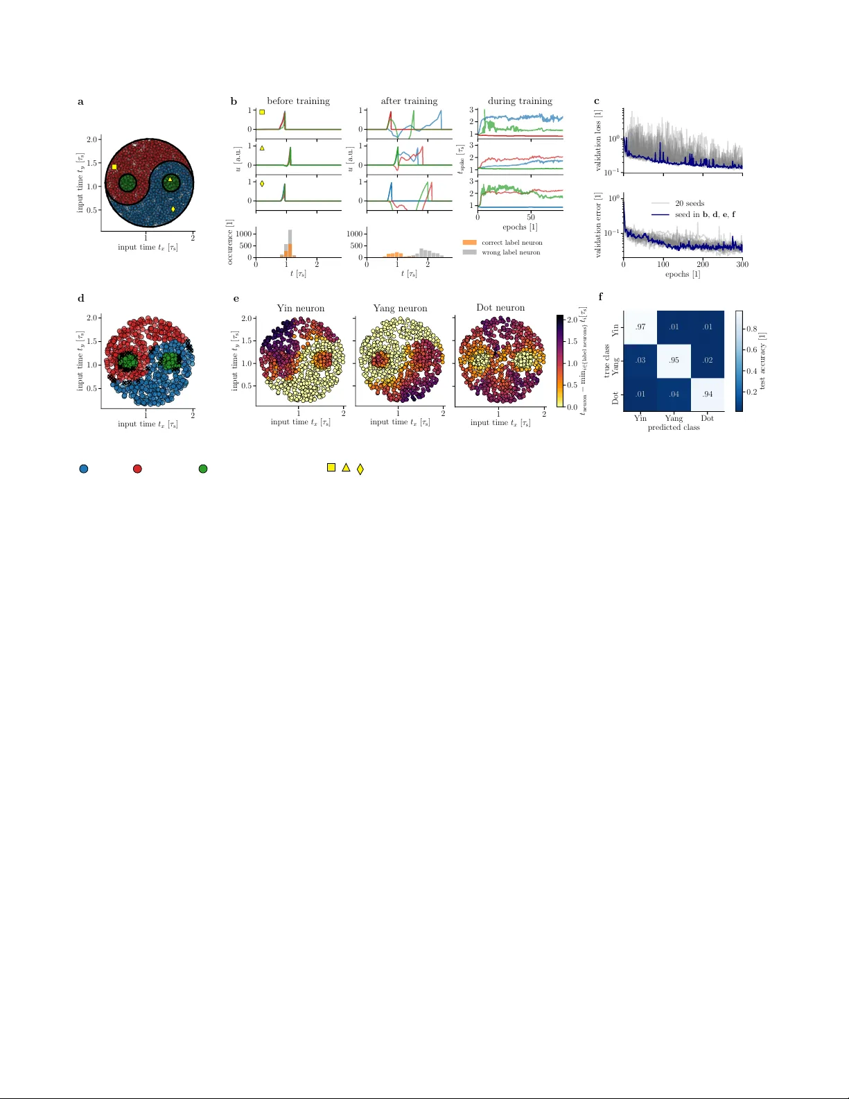
F ast and energy-eﬃcien t neuromorphic deep learning with ﬁrst-spik e times J. G¨ oltz ∗ , ¶ , 1 , 2 , L. Kriener ∗ , ¶ , 2 , A. Baum bac h 1 , S. Billaudelle 1 , O. Breit wieser 1 , B. Cramer 1 , D. Dold 1 , 3 , A. F. Kungl 1 , W. Senn 2 , J. Sc hemmel 1 , K. Meier † , 1 , M. A. P etro vici ¶ , 2 , 1 ∗ Shared ﬁrst authorship † Deceased ¶ Corresponding authors (julian.go eltz@kip.uni-heidelberg.de, { laura.kriener,mihai.p etro vici } @unib e.c h) 1 Kirchhoﬀ-Institute for Physics, Heidelberg University , 69120 Heidelberg, Germany . 2 Department of Physiology , University of Bern, 3012 Bern, Switzerland. 3 Siemens AI lab, Siemens AG T echnology , 80331 Munich, German y . Abstract F or a biolo gic al agent op er ating under envir onmental pr es- sur e, ener gy c onsumption and r e action times ar e of criti- c al imp ortanc e. Similarly, engine er e d systems ar e optimize d for short time-to-solution and low ener gy-to-solution char- acteristics. A t the level of neur onal implementation, this implies achieving the desir e d r esults with as few and as e arly spikes as p ossible. With time-to-ﬁrst-spike c o ding b oth of these go als ar e inher ently emer ging fe atur es of le arning. Her e, we describ e a rigor ous derivation of a le arning rule for such ﬁrst-spike times in networks of le aky inte gr ate-and- ﬁr e neur ons, r elying solely on input and output spike times, and show how this me chanism c an implement err or b ack- pr op agation in hier ar chic al spiking networks. F urthermor e, we emulate our fr amework on the Br ainSc aleS-2 neur omor- phic system and demonstr ate its c ap ability of harnessing the system’s sp e e d and ener gy char acteristics. Final ly, we ex- amine how our appr o ach gener alizes to other neur omorphic platforms by studying how its p erformanc e is aﬀe cte d by typ- ic al distortive eﬀe cts induc e d by neur omorphic substr ates. In tro duction In recen t years, the machine learning landscape has b een dominated by deep learning metho ds. Among the b enc h- mark problems they managed to crack, some were though t to still remain elusiv e for a long time [1–3]. It is thus not exaggerated to say that deep learning dominates our under- standing of “artiﬁcial in telligence” [4–8]. Compared to abstract neural net w orks used in deep learn- ing, their more biological archet yp es — spiking neural net- w orks — still lag b ehind in p erformance and scalability [9]. Reasons for this diﬀerence in success are numerous; for instance, unlik e abstract neurons, even an individual bi- ological neuron represen ts a complex system, with ﬁnite re- sp onse times, membrane dynamics and spik e-based comm u- nication [10, 11], making it more challenging to ﬁnd reliable co ding and computation paradigms [12–14]. F urthermore, one of the ma jor driving forces b ehind the success of deep learning, the backpropagation of errors algorithm [15–17], remained incompatible with spiking neural netw orks until only v ery recen tly [18, 19]. Despite these c hallenges, spiking neural net works promise to hold some imp ortan t adv antages. The time informa- tion inherent to spikes allows a co ding scheme for spike- based communication that utilizes b oth spatial and tem- p oral dimensions [20], unlik e spike-coun t-based approaches [21–24], where the information of spike times is at least par- tially diluted due to temporal or p opulation a v eraging. Ow- ing to the inheren t parallelism of all biological, as well as man y biologically-inspired, spiking neuromorphic systems [25], this promises fast, sparse and energy-eﬃcient infor- mation pro cessing, and provides a blueprint for comput- ing arc hitectures that could one da y riv al the eﬃciency of the brain itself [9, 25–27]. This makes spiking neural net- w orks implemen ted on sp ecialised neuromorphic devices po- ten tially more p o werful — at least in principle — than the “con v entional”, simple mac hine learning mo dels currently used on v on-Neumann mac hines, even though this potential still remains mostly unexploited [9]. Man y attempts ha ve b een made to reconcile spiking neu- ral netw orks with their abstract counterparts in terms of functionalit y , e.g., featuring spike-based inference mo dels [28–36] and deep mo dels trained on target spik e times b y shallo w learning rules [37, 38] or using spik e-compatible v er- sions of the error backpropagation algorithm [39–41]. Es- p ecially for tasks op erating on static information, a partic- ularly elegan t wa y of utilizing the temp oral asp ect of exact spik e times is the time-to-ﬁrst-spik e (TTFS) co ding scheme [42]. Here, a neuron enco des its real-v alued resp onse to a stim ulus as the time elapsed b efore its ﬁrst spik e in reaction to that stimulus. Suc h single-spik e co ding enables fast in- formation pro cessing b y explicitly encouraging the emission 1 of as few spikes as early as p ossible, which meets ph ysiolog- ical constrain ts and reaction times observed in humans and animals [42–45]. Apart from biological plausibility , suc h a fast and sparse co ding scheme is a natural ﬁt for neuromor- phic systems that oﬀer energy-eﬃcient and fast em ulation of spiking neural net w orks [46–52]. F or hierarchical TTFS netw orks, a gradient-descen t- based learning rule was prop osed in [53, 54], using error bac kpropagation on a contin uous function of output spike times. Ho wev er, this approach is limited to a neuron model without leak, which is neither biologically plausible, nor compatible with most analog v ery-large-scale in tegration (VLSI) neuron dynamics [25]. W e prop ose a solution for leaky integrate-and-ﬁre (LIF) neurons with current-based (CuBa) synapses — a widely-used dynamical mo del of spik- ing neurons with realistic in tegration b eha vior [55–57]. An early v ersion of this w ork w as presen ted in G¨ oltz [58]. F or several speciﬁc conﬁgurations of time constan ts, we pro vide analytical expressions for ﬁrst-spik e timing, which, in turn, allow the calculation of exact gradients of any dif- feren tiable cost function that dep ends on these spik e times. In hierarchical netw orks of LIF neurons using the TTFS co ding scheme, this enables exact error backpropagation, allo wing us to train such netw orks as universal classiﬁers on b oth con tinuous and discrete data spaces. As our algorithm only requires knowledge ab out aﬀer- en t and eﬀerent spik e times of all neurons, it lends itself to emulation on neuromorphic hardware. The accelerated, y et pow er-eﬃcient BrainScaleS-2 platform [48, 59] pairs es- p ecially well with the sparseness and low latency already inheren t to TTFS co ding. W e show ho w an implementation of our algorithm on BrainScaleS-2 can obtain similar classi- ﬁcation accuracies to softw are sim ulations, while displaying highly comp etitiv e time and pow er c haracteristics, with a com bination of 48 µ s and 8.4 µ J p er classiﬁcation. By incorporating information generated on the hardw are for up dates during training, the algorithm automatically adapts to p oten tial imp erfections of neuromorphic circuits, as implicitly demonstrated b y our neuromorphic implemen- tation. In further softw are simulations, we show that our mo del deals well with v arious levels of substrate-induced dis- tortions such as ﬁxed-pattern noise and limited parameter precision and control, thus providing a rigorous algorith- mic backbone for a wide range of neuromorphic substrates and applications. Suc h robustness with resp ect to imper- fections of the underlying neuronal substrate represents an indisp ensable prop ert y for any netw ork mo del aiming for biological plausibility and for every application geared to- w ards ph ysical computing systems [33, 34, 60–64]. In the following, we ﬁrst in tro duce the CuBa LIF mo del and the TTFS co ding sc heme, b efore w e demonstrate ho w time [a. u.] PSPs [a. u.] τ m /τ s → ∞ τ m /τ s = 2 τ m /τ s = 1 τ m /τ s → 0 a time [a.u.] neuron id d c ϑ E ` b time [a. u.] ϑ E ` mem brane v oltage Figure 1: Time-to-ﬁrst-spike co ding and learning. T op: sin- gle neurons. (a) P ostsynaptic potential (PSP) shapes for diﬀeren t ratios of time constants τ s and τ m . The ﬁniteness of time constants causes the neuron to gradually forget prior input. (b) One k ey c hal- lenge of this ﬁnite memory arises when small v ariations of the synaptic weigh ts result in disappearing/app earing output spik es, which elicits a discontin uity in the function describing output spike timing. Bottom: application to feedforw ard hierarc hical netw orks. (c) Netw ork structure. The geometric shape of the neurons represents a notation of their resp ectiv e t yp es (input  , hidden ◦ , label 4 ). The shading of the input neurons is a representation of the corresp onding data, such as pixel brightness (  , . . . ,  , . . . ,  ). The color of the lab el neu- rons represen ts their respective class ( N , N , N ). (d) Time-to-ﬁrst-spik e (TTFS) coding exempliﬁed in a raster plot. As an example of input encoding, the brightness of an input pixel is enco ded in the lateness of a spike. Note that in our framework, TTFS co ding simultaneously refers to t wo individual asp ects, namely the input-to-spike-time con- version and the determination of the inferred class b y the identit y of the ﬁrst lab el neuron to ﬁre ( N ). In all ﬁgures w e denote units in square brac kets; in particular, w e use [a. u.] for arbitrary units, and [1] for dimensionless quantities, and [ τ s ] for times that are measured in multiples of the synaptic time constant τ s . b oth inference and training via error bac kpropagation can b e p erformed analytically with such dynamics. Finally , the presen ted mo del is ev aluated b oth in soft ware sim ulations and neuromorphic em ulations, before studying eﬀects of sev- eral t yp es of substrate-induced distortions. Results Leaky integrate-and-ﬁre dynamics The dynamics of an LIF neuron with CuBa synapses are giv en b y C m ˙ u ( t ) = g ` [ E ` − u ( t )] + X i w i X t i θ ( t − t i ) exp  − t − t i τ s  , (1) with membrane capacitance C m , leak conductance g ` (from whic h the membrane time constant τ m = C m /g ` follo ws), presynaptic weigh ts w i and spike times t i , synaptic time 2 constan t τ s and θ the Hea viside step function. The ﬁrst sum runs o ver all presynaptic neurons while the second sum runs o ver all spik es for eac h presynaptic neuron. The neuron elicits a spike at time T when the presynaptic input pushes the membrane potential abov e a threshold ϑ . After spiking, a neuron b ecomes refractory for a time p eriod τ ref , which is modeled by clamping its mem brane p oten tial to a reset v alue % : u ( t 0 ) = % for T ≤ t 0 ≤ T + τ ref . F or conv enience and without loss of generalit y , we set the leak p oten tial E ` = 0. Eqn. (1) can b e solv ed analytically and yields subthreshold dynamics as describ ed by Eqn. (9). The choice of τ m and τ s ultimately inﬂuences the shap e of a postsynaptic p oten tial (PSP), starting from a simple exp onen tial ( τ m  τ s ), to a diﬀerence of exponentials (with an alpha function for the sp ecial case of τ m = τ s ) to a graded step function ( τ m  τ s ) (Fig. 1a). Note that all of these scenarios are conserv ed un- der exc hange of τ s and τ m , as is apparent from the symmetry of the analytical solution (Eqn. (9)). The ﬁrst tw o cases with ﬁnite mem brane time constan t τ m are mark edly diﬀeren t from the last one, which is also kno wn as either the non-leaky integrate-and-ﬁre (nLIF) or simply integrate-and-ﬁre (IF) model and was used in previ- ous w ork [53]. In the nLIF model, input to the membrane is nev er forgotten un til a neuron spikes, as opp osed to the LIF mo del, where the PSP reaches a p eak after ﬁnite time and subsequen tly decays back to its baseline. In other w ords, presynaptic spikes in the LIF model hav e a purely lo cal ef- fect in time, unlike in the nLIF mo del, where only the onset of a PSP is localized in time, but the p ostsynaptic eﬀect remains forev er, or until the p ostsynaptic neuron spik es. A pair of ﬁnite time constants thus assigns muc h more im- p ortance to the time diﬀerences b et w een input spik es and in tro duces discon tinuities in the neuronal output that mak e an analytical treatmen t more diﬃcult (Fig. 1b). First-spik e times Our spike-timing-based neural co de follo ws an idea ﬁrst prop osed in [53]. Unlike co ding in artiﬁcial neural netw orks (ANNs) and diﬀeren t from spike- coun t-based co des in spiking neural net works (SNNs), this sc heme explicitly uses the timing of individual spikes for enco ding information. In time-to-ﬁrst-spik e (TTFS) co d- ing, the presence of a feature in a stimulus is reﬂected by the timing of a neuron’s ﬁrst spike after the onset of the stim ulus , with earlier spik es represen ting a more strongly manifested feature. This has the eﬀect that important infor- mation inheren tly propagates quic kly through the net work, with p oten tially only few spikes needed for the netw ork to pro cess an input. Consequen tly , this scheme enables eﬃ- cien t pro cessing of inputs, both in terms of time-to-solution and energy-to-solution (assuming the latter depends, in gen- eral on the total num b er of spik es and the time requi red for the net w ork to solv e, e.g., an input classiﬁcation problem). In order to formulate the optimization of a ﬁrst-spike time T as a gradient-descen t problem, we deriv e an ana- lytical expression for T . This is equiv alen t to ﬁnding the time of the ﬁrst threshold crossing b y solving u ( T ) = ϑ for T . Ev en though there is no general closed-form solution for this problem, analytical solutions exist for sp eciﬁc cases. F or example, we sho w that (see Metho ds) T = τ s  b a 1 − W  − g ` ϑ a 1 exp  b a 1  for τ m = τ s (2) and T = 2 τ s ln " 2 a 1 a 2 + p a 2 2 − 4 a 1 g ` ϑ # for τ m = 2 τ s , (3) where W is the Lambert W function and using the shorthand notations a n and b for sums ov er the set of causal presynaptic spikes C = { i | t i < T } (see Eqns. (11) and (12)). W e note that, when calculating the output spik e time for a large num b er of input neurons, determining C can be computationally in tensiv e (see Metho ds). One in- heren t adv antage of ph ysical em ulation is the reduction of this calculational burden. The ab o ve equations are diﬀerentiable with resp ect to synaptic w eights and presynaptic spike times. As will b e sho wn in the following, this directly translates to solving the credit assignment problem and thus allo ws exact error propagation through net works of spiking neurons. F or eas- ier reading, we fo cus on one speciﬁc case ( τ m = τ s ), but the others can b e treated analogously . Exact error backpropagation with spikes Learning in SNNs requires the ability to relate eﬀerent spiking to b oth aﬀerent weigh ts and spike times. F or the output spike time of a neuron k with presynaptic partners i , the ﬁrst re- lationship can be formally described b y the deriv ativ e of the output spik e time with respect to the presynaptic w eights (Eqn. (22)). Using certain properties of W , we can ﬁnd a simple expression that can, additionally , b e made to depend on the output spik e time t k itself: ∂ t k ∂ w ki = − 1 a 1 exp  t i τ s  W ( z ) + 1 ( t k − t i ) , (4) with a 1 and z representing functions of w ki and t i as deﬁned in Eqns. (11) and (18). Using the output spik e time as ad- ditional information optimizes learning in scenarios where the exact neuron parameters are unkno wn and the real out- put spike time diﬀers from the one calculated under ideal assumptions, as discussed later. 3 Second, the capabilit y to relate errors in the output spike time to errors in the input spik e times allo ws us to recur- siv ely propagate c hanges from neurons to their presynaptic partners. ∂ t k ∂ t i = − 1 a 1 exp  t i τ s  W ( z ) + 1 w ki τ s ( t k − t i − τ s ) . (5) T ogether, Eqns. (4) and (5) eﬀectively and exactly solv e the credit assignment problem in appropriately parametrized LIF net w orks of arbitrary arc hitecture. W e can now apply the ﬁndings ab o ve to study learning in a lay ered netw ork. Figure 1c sho ws a sc hematic of our feed- forw ard netw orks and their spiking activity . The input uses the same co ding scheme as all other neurons: more promi- nen t features are enco ded by earlier spikes. The output of the netw ork is deﬁned by the iden tity of the lab el neuron that spik es ﬁrst (Fig. 1d). W e denote by t ( l ) k the output spik e time of the k th neuron in the l th lay er; for example, in a netw ork with N lay ers, t ( N ) n is the spike time of the n th neuron in the lab el la yer. The w eight pro jecting to the k th neuron of lay er l from the i th neuron of la y er l − 1 is denoted by w ( l ) ki . T o apply the error bac kpropagation algorithm [15, 17], w e c ho ose a loss function that is diﬀeren tiable with resp ect to synaptic w eights and spike times. During learning, the ob jective is to maximize the temp oral diﬀerence b et ween the correct and all other lab el spik es. The following loss function fulﬁlls the ab o ve requiremen ts: L [ t ( N ) , n ∗ ] = dist  t ( N ) n ∗ , t ( N ) n 6 = n ∗  = log " X n exp − t ( N ) n − t ( N ) n ∗ ξ τ s !# , (6) where t ( N ) denotes the vector of lab el spike times t ( N ) n , n ∗ the index of the correct label and ξ ∈ R + is a scaling param- eter. This loss function represen ts a cross entrop y b etw een the true label distribution and the softmax-scaled lab el spike times produced b y the net work (see Metho ds). Reducing its v alue therefore increases the temp oral diﬀerence b et ween the output spike of the correct label neuron and all other lab el neurons. Notably , it only dep ends on the spik e time diﬀerence and is in v arian t under absolute time shifts, mak- ing it independent of the concrete c hoice of the experiment start which deﬁnes t = 0. In case of a non-spiking lab el neuron we treat its spike time as t ( N ) n = ∞ . In this case ho w ever, the equation Eqn. (2) is not deﬁned and neither are its deriv ativ es. W e therefore in tro duce a simple, lo cal heuristic to encourage spiking b eha viour in large p ortions of the net work (see Metho ds). In some scenarios, learning can b e facilitated b y the addition of a spik e-time-dep enden t regularization term (see Metho ds). Gradien t descen t on the loss function Eqn. (6) can now be easily p erformed by rep eated application of the chain rule. Using the exact deriv atives Eqns. (4) and (5), this yields the synaptic plasticit y rule ∆ w ( l ) ki ∝ − ∂ L [ t ( N ) , n ∗ ] ∂ w ( l ) ki (7) = − ∂ t ( l ) k ∂ w ( l ) ki ∂ L [ t ( N ) , n ∗ ] ∂ t ( l ) k | {z } δ ( l ) k = − ∂ t ( l ) k ∂ w ( l ) ki X j ∂ t ( l +1) j ∂ t ( l ) k δ ( l +1) j . A compact form ulation for hierarchical netw orks that highligh ts the backpropagation of errors can b e found in Eqns. (38) to (40). In either form, only the lab el la yer error and the neuron spike times are required for training, whic h can either be calculated using Eqn. (2) or b y simulating (or em ulating) the LIF dynamics (Eqn. (1)). The computational complexity of the synaptic plasticit y rule – a p oten tial limiting factor for on-chip implementa- tions – can be drastically reduced by appropriate approxi- mations. In the Supplementary Information SI.D w e presen t early results using suc h an approac h. Note that the simpliﬁ- cation is only used in Supplementary Information SI.D and all other results we report in the following w ere pro duced using the full analytical equations Eqns. (4) and (5). Sim ulations After deriving the learning algorithm in the previous c hapter, we show its classiﬁcation capabilities in soft w are sim ulations. In these sim ulations we demonstrate successful learning and provide a baseline for the hardw are em ulations that follo w. W e use tw o data sets that emphasize diﬀerent aspects of in teresting real-w orld scenarios. As an example for lo w-dimensional, “con tin uous” data spaces, in which p oin ts b elonging to diﬀerent classes can b e arbitrarily close together (thus making separation par- ticularly c hallenging), we c hose the Yin-Y ang data set [65]. F or higher-dimensional, discrete input, w e used the MNIST data set [66] as a small-scale image classiﬁcation scenario. The results in this section are based on Eqn. (2) for calcu- lating the spike times in the forw ard pass, and Eqn. (40) for calculating weigh t updates; for details regarding implemen- tation see Methods. F or hyperparameters of the discussed exp erimen ts see T ables A and B. Yin-Y ang classiﬁc ation task: The ﬁrst data set consists of p oin ts in the yi n-y ang ﬁgure (Fig. 2a). Each p oin t is deﬁned b y a pair of Cartesian coordinates ( x, y ) ∈ [0 , 1] 2 . T o build in redundancy and capture the intrinsic symmetry of the 4 1 2 input time t x [ τ s ] Y ang neuron 10 − 1 10 0 v alidation loss [1] c 0 100 200 300 ep o c hs [1] 10 − 1 10 0 v alidation error [1] 20 seeds seed in b , d , e , f 1 2 input time t x [ τ s ] 0 . 5 1 . 0 1 . 5 2 . 0 input time t y [ τ s ] Yin neuron e 1 2 3 t spik e [ τ s ] 1 2 3 during training 1 2 input time t x [ τ s ] Dot neuron 0 1 0 1 1 2 input time t x [ τ s ] 0 . 5 1 . 0 1 . 5 2 . 0 input time t y [ τ s ] d 1 2 input time t x [ τ s ] 0 . 5 1 . 0 1 . 5 2 . 0 input time t y [ τ s ] a 0 50 ep o c hs [1] 1 2 3 0 1 u [ a.u.] 0 1 u [ a.u.] 0 1 after training 0 1 b efore training b 0 1 2 t [ τ s ] 0 500 1000 o ccurence [1] 0 1 2 t [ τ s ] 0 500 1000 correct lab el neuron wrong lab el neuron Yin Y ang Dot predicted class Yin Y ang Dot true class .97 .01 .01 .03 .95 .02 .01 .04 .94 f 0 . 0 0 . 5 1 . 0 1 . 5 2 . 0 t neuron − min i ∈{ lab el neurons } t i [ τ s ] 0 . 2 0 . 4 0 . 6 0 . 8 test accuracy [1] Figure 2: Classiﬁcation of the Yin-Y ang data set. (a) Illustration of the Yin-Y ang data set. The samples are separated into three classes, Yin ( ), Y ang ( ) and Dot ( ). The y ellow sym b ols ( , , ) mark samples for which the training process is illustrated in (b). The input times t x and t y correspond to the spike time of the inputs asso ciated with the x and y co ordinates of individual samples. (b) T raining mechanism for three exemplary data samples (cf. (a)). F or the ﬁrst three rows, the left and middle columns depict voltage dynamics in the lab el lay er before and after training for 300 ep ochs, resp ectiv ely . The voltage traces of the three lab el neurons are color-co ded according to their corresp onding class as in (a). Before training, the random initialization of the weights causes the lab el neurons to show similar voltage traces and almost indistinguishable spike times. After training there is a clear separation b et ween the spik e time of the correct lab el neuron and all others, with the correct neuron spiking ﬁrst. The evolution of the label spik e times during training is shown in the right column for the ﬁrst 70 epo c hs. Bottom row: spike histograms ov er all training samples. Our learning algorithm induces a clear separation b et ween the spike times of correct and wrong lab el neurons. (c) T raining progress (v alidation loss as giv en in Eqn. (6) and error rate) over 300 ep ochs for 20 training runs with random initializations (gra y). The run shown in panels b and d-f is plotted in blue. (d) Classiﬁcation result on the test set (1000 samples). The color of eac h sample indicates the class determined b y the trained netw ork. The wrongly classiﬁed samples (mark ed with blac k X) all lie very close to the b order betw een classes. (e) Spik e times of the Yin, Y ang and Dot neurons for all test samples after training. F or each sample, spike times were normalized by subtracting the earliest spike time in the lab el la yer. Bright y ellow denotes zero diﬀerence, i.e., the respective lab el neuron w as the ﬁrst to spike and the sample w as assigned to its class. The bright yello w areas resemble the shap es of the Yin, Y ang and Dot areas, reﬂecting the high classiﬁcation accuracy after training. (f ) Confusion matrix for the test set after training. yin-y ang motive, the data set is augmented with mirrored co ordinates (1 − x, 1 − y ) enabling net works of neurons with- out trainable bias to learn the task [65]. The three classes are lab eled as per the respective area they occupy , i.e., Yin, Y ang or Dot. This augmen ted data set w as sp eciﬁcally de- signed to require latent v ariables for classiﬁcation: a shallo w non-spiking classiﬁer reaches (64 . 3 ± 0 . 2)% test accuracy , an ANN with one hidden lay er of size 120 typically around (98 . 7 ± 0 . 3)%. Due to this large gap, our Yin-Y ang data set represents an expressive test of error backpropagation in our hierarc hical spiking net w orks. At the same time, it can b e learned by net works that are compatible in size with the curren t revision of BrainScaleS-2 [67]. After translation of the four features to spike times (see Fig. 1 and Metho ds for more details), they w ere joined with a bias spike at ﬁxed time, and these ﬁv e spikes served as in- put to a netw ork with 120 hidden and 3 lab el neurons. W e illustrate the training me c hanism with v oltage traces for three samples b elonging to diﬀerent classes (Fig. 2b). The algorithm c hanges the w eights to create a separation in the lab el spike times (cf. left and middle column) that corre- sp onds to correct classiﬁcation. Note that the v oltage traces w ere just recorded for illustration, as only spike times are required for calculating w eight updates. After 300 ep ochs our net works reached (95 . 9 ± 0 . 7)% test accuracy for training with 20 diﬀeren t random seeds (Fig. 2c). The classiﬁcation failed only for samples that w ere extremely close to the b or- der betw een t wo classes (Fig. 2d). Figure 2e sho ws the spike times of the lab el neurons. These v ary contin uously for in- puts b elonging to other classes, but drop abruptly at the b oundary of the area b elonging to their o wn class, which denotes a clear separation – see, for example, the abrupt c hange from red (late spike time) to yello w (early spike time) of the Yin-neuron when mo ving from Y ang to Yin (Fig. 2e, 5 left panel). 0 50 100 150 ep o c hs [1] 10 − 1 10 0 v alidation error [1] 0 50 100 150 10 − 1 10 0 v alidation loss [1] 10 seeds seed in b a 0 1 2 3 4 5 6 7 8 9 predicted class 0 1 2 3 4 5 6 7 8 9 true class .98 .00 .00 .00 .00 .00 .01 .00 .01 .00 .00 .99 .00 .00 .00 .00 .00 .00 .00 .00 .00 .00 .96 .01 .00 .00 .01 .00 .02 .00 .00 .00 .00 .97 .00 .01 .00 .00 .01 .00 .00 .00 .00 .00 .98 .00 .01 .00 .00 .01 .00 .00 .00 .01 .00 .97 .01 .00 .01 .00 .00 .00 .00 .00 .00 .00 .98 .00 .00 .00 .00 .01 .01 .00 .00 .00 .00 .96 .01 .00 .00 .00 .00 .00 .00 .00 .00 .01 .98 .00 .00 .00 .00 .00 .01 .01 .00 .01 .02 .93 b 0 . 0 0 . 2 0 . 4 0 . 6 0 . 8 test accuracy [1] Figure 3: Classiﬁcation of the MNIST data set. (a) T raining progress of a netw ork ov er 150 epochs for 10 diﬀerent random initial- izations. The run dra wn in blue is the one whic h pro duced the results in (b). (b) Confusion matrix for the test set after training. MNIST classiﬁc ation task: T o study the scalabilit y of our approac h to larger and more high-dimensional data sets, w e applied it to the classiﬁcation of MNIST handwritten digits [66]. Figure 3 shows training results for net works with 784- 350-10 neurons, where pixel intensities were translated to spik e times. During training, noise was added to the input samples to aid generalization, but no bias spikes were used. As seen in Fig. 3a, training con verges for 10 diﬀerent initial random seeds, reac hing a ﬁnal test accuracy of (97 . 1 ± 0 . 1)%. Similar results are also achiev ed for deep er architectures with multiple hidden lay ers (see T able SI.B1 for additional sim ulation runs with diﬀeren t net w ork architectures). F or reference, we consider sev eral other results obtained with spiking-time co ding. In Mostafa [53], a maxim um test accuracy of 97 . 55% using a netw ork with a hidden la yer of 800 neurons is reported; note that this w ork uses non-leaky neurons with eﬀectively inﬁnite membrane memory . Also for non-leaky neurons, but using an appro ximative approach for calculating gradien ts, Kheradpisheh & Masquelier [54] rep ort 97 . 4% using 400 hidden neurons. In Comsa et al. [68], a maxim um test accuracy of 97 . 96% w as ac hieved using 340 hidden neurons, supp orted by a regular spike grid and extensiv e h yp erparameter searc h. W e note that there also exist trial-av eraging and spike- coun t-based approaches that hav e the b eneﬁt of more straigh t-forw ard learning rules, but these approaches sac- riﬁce precision, neuronal real-estate or time-to-solution in comparison to framew orks based on the precise timing of single output spik es. F or example, Esser et al. [61] rep ort 92 . 7% using 512 neu- rons, while T av anaei et al. [69] require 1000 hidden neurons to ac hiev e 96 . 6%. F ast neuromorphic classiﬁcation In our framework, the time to solution is a function of the net work depth and the time constan ts τ m and τ s . Assuming typical biologi- cal timescales, most input patterns in the ab o ve scenario are classiﬁed within several milliseconds. By leveraging the sp eedup of neuromorphic systems such as BrainScaleS [46, 67], with intrinsic acceleration factors of 10 3 to 10 4 , the same computation can b e ac hieved within microseconds. In the following, we presen t an implementation of our frame- w ork on BrainScaleS-2 and discuss its p erformance in con- junction with the achiev ed classiﬁcation sp eed and energy consumption. F or a pro of-of-concept implemen tation on its predecessor BrainScaleS-1, we refer to Supplementary In- formation SI.A. The adv antages of such a neuromorphic implementation come at the cost of reduced control. T raining needs to cop e with phenomena such as spike jitter, limited weigh t range and granularit y , as well as neuron parameter v ariability , among others. In general, an imp ortan t aspect of any theory aiming for compatibilit y with physical substrates, b e they biological or artiﬁcial, is its robustness to substrate imp er- fections; our results on BrainScaleS-2 implicitly represent a p o werful demonstration of this prop ert y . T o further sub- stan tiate the generalizability of our algorithm to diﬀerent substrates, we complement our exp erimen tal results with a sim ulation study of v arious substrate-induced distortive eﬀects. L e arning on Br ainSc aleS-2: BrainScaleS-2 is a mixed- signal accelerated neuromorphic platform with 512 phys- ical neurons, each being able to receive inputs via 256 conﬁgurable synapses. These neurons can b e coupled to form larger logical neurons with a correspondingly increased n um b er of inputs. At the heart of eac h neuron is an analog circuit emulating LIF neuronal dynamics with an accelera- tion factor of 10 3 to 10 4 compared to biological timescales. Due to v ariations in the man ufacturing process, the real- ized circuits systematically deviate from each other (ﬁxed- pattern noise). Although these v ariations can b e reduced b y calibrating each circuit [72], considerable diﬀerences remain (standard deviation on the order of 5 % on BrainScaleS-2) and p ose a challenge for p ossible neuromorphic algorithms – along with other features of physical mo del systems suc h as spik e time jitter or spik e loss [33, 34, 63, 73]. The chip’s synaptic arrays w ere conﬁgured to supp ort ar- bitrary fully-connected net w orks of up to 256 emulated neu- rons with a maxim um of 256 inputs per neuron. Eac h suc h logical connection was realized via t w o physical synapses in order to allo w transitions b et ween an excitatory and an inhibitory regime. Synaptic w eights on the chip are conﬁg- urable with 6 bit precision. More details ab out our setup can b e found in the Methods section. W e used an in-the-lo op training approach [23, 33, 74], where inference runs emulated on the neuromorphic sub- 6 0 20 40 ep o c hs [1] 10 − 1 10 0 v alidation error [1] 10 seeds run in g , h 10 0 10 − 1 v alidation loss [1] b 0 20 40 10 0 10 − 1 v alidation loss [1] f Yin Y ang Dot predicted class Yin Y ang Dot true class .95 .03 .02 .02 .96 .03 .03 .03 .95 c 0 1 2 3 4 5 6 7 8 9 predicted class 0 1 2 3 4 5 6 7 8 9 true class .99 .00 .00 .00 .00 .00 .00 .00 .00 .00 .00 .98 .00 .00 .00 .00 .00 .00 .00 .00 .01 .00 .97 .00 .00 .00 .00 .01 .00 .00 .00 .00 .01 .96 .00 .01 .00 .00 .01 .01 .00 .00 .00 .00 .97 .00 .01 .00 .00 .01 .00 .00 .00 .01 .00 .97 .00 .00 .00 .01 .01 .00 .00 .00 .01 .01 .97 .00 .00 .00 .00 .00 .01 .00 .00 .00 .00 .98 .00 .00 .01 .00 .01 .00 .00 .01 .00 .01 .95 .01 .00 .00 .00 .00 .03 .00 .00 .01 .00 .95 g 5 10 input time t x [ µ s] Y ang neuron a 5 10 input time t x [ µ s] 5 10 input time t y [ µ s] d 5 10 input time t x [ µ s] 5 10 input time t y [ µ s] Yin neuron e 5 10 input time t x [ µ s] Dot neuron 0 200 400 ep o c hs [1] 10 − 1 10 0 v alidation error [1] 10 seeds run in c , d , e u [a. u.] 3 0 10 20 time [ µ s] u [a. u.] 8 u [a. u.] 0 h u [a. u.] 1 0 . 2 0 . 4 0 . 6 0 . 8 test accuracy [1] 0 2 4 6 8 10 12 t neuron − min i ∈{ lab el neurons } t i [ µ s] 0 . 0 0 . 2 0 . 4 0 . 6 0 . 8 test accuracy [1] BrainScaleS-2 ASIC Figure 4: Classiﬁcation on the BrainScaleS-2 neuromorphic platform. (a) Photograph of a BrainScaleS-2 c hip. (b-e) Yin-Y ang data set (b) T raining progress ov er 200 ep ochs for 11 diﬀeren t random initializations. The run dra wn in blue also pro duced the results sho wn in panel (b-d). (c) Confusion matrix for the test set after training. (d) Classiﬁcation result on the test set. F or each input sample the color indicates the class determined b y the trained net work. W rong classiﬁcations are marked with a black X. The wrongly classiﬁed samples all lie v ery close to the border b et ween tw o classes. (e) Separation of label spike times (cf. Fig. 2e). F or each of the label neurons, bright yello w dots represent data samples for which it w as the ﬁrst to spike, thereby assigning them its class. Similarly to the soft ware simulations, the bright yello w areas align well with the shap es of the Yin, Y ang and Dot areas of the data set. (f-h) MNIST data set (f ) Ev olution of training ov er 50 epo c hs for 10 diﬀerent random initializations. The run drawn in blue is the one which produced the results sho wn in panel (g) and (h). (g) Confusion matrix for the test set after training. (h) Exemplary mem brane voltage traces on BrainScaleS-2 after training. Eac h panel sho ws color-coded voltage traces of four lab el neurons for one input that w as presented repeatedly to the net work (inla ys sho w the input and its correct class). Each trace was recorded four times to p oin t out the trial-to-trial v ariations. strate were interlea ved with host-based weigh t update cal- culations. F or em ulating the forward pass, the spike times for eac h sample in a mini-batc h w ere joined sequentially in to one long spik e train and then injected into the neuromor- phic system via a ﬁeld-programmable gate array (FPGA). The latter was also used to record the spikes emitted by the hidden and lab el la yers. Figure 4a-d sho ws the results of training a spiking netw ork with 120 hidden neurons on BrainScaleS-2 on the Yin-Y ang data set. The system quic kly learned to discriminate b e- t w e en the presen ted patterns, with an av erage test accuracy of (95 . 0 ± 0 . 9)%. The hardware emulation performs similarly to the soft- w are sim ulations (Fig. 2), with the wrong classiﬁcations still only happening along the b orders of the areas with diﬀeren t lab els (Fig. 4c). The remaining diﬀerence in p erformance after training is attributable to the substrate v ariability (cf. also Fig. 4h). Considering that one of the speciﬁc c hallenges built into the Yin-Y ang data set resides in the con tinuit y of its input space and abrupt class switc h b et w een b ordering areas, this result highligh ts the robustness of our approac h. T o classify the MNIST data set using the BrainScaleS-2 system, we emulated and trained a netw ork of size 256-246- 10 (Fig. 4f-h). Due to the restrictions imp osed by the hard- w are on the input dimensionality , we used downsampled images of 16 × 16 pixels. Across multiple initializations, we ac hiev e d a test accuracy of (96 . 9 ± 0 . 1)%; similarly to the Yin-Y ang data set, this is only slightly low er than in soft- w are sim ulations of equally sized netw orks (T able 2). As sho wn in T able 2, ab out one third of the loss in accuracy is due to the do wnsampling of the data, with the remainder b eing caused by the v ariability of the substrate. The abil- it y of our framework to achiev e reliable classiﬁcation de- spite such substrate-induced distortions is well-illustrated b y p ost-training membrane dynamics measured on the chip Fig. 4h. In all cases shown here, the correct lab el neuron spik es before 10 µ s and is clearly separable from all other lab el neurons. Due to its short intrinsic time constants and ov erall energy eﬃciency , the BrainScaleS-2 system enables very fast and e n ergy-eﬃcien t acquisition of classiﬁcation results. Classiﬁcation of the 10 000 MNIST test samples tak es a total of 0.937 s, including data transmission, em ulation of dynam- ics and return of the classiﬁcation results. The total time on the BrainScaleS-2 c hip w as 480 µ s, a detailed breakdown of the execution time is shown in Supplementary Informa- tion SI.E. The p o wer consumption of the c hip, measured during run time, including all c hip comp onen ts needed for spik e generation and processing (i.e., excluding the host and FPGA) amoun ted to 175 mW. F or measuremen t details and 7 T able 1: Comparison of pattern recognition mo dels on the MNIST data set emulated on neuromorphic back-ends, sorted b y classiﬁcation sp eed. F or reference, an ANN running on GPU is included in the top row. Note that w e include only references which present measurements for both energy and throughput in addition to accuracy . An extended table con taining results with partial or estimated measuremen ts can be found in Supplementary Information, T able SI.F1. platform type technology co ding input netw ork data augmentation/ energy p er classiﬁcations test reference resolution size/structure regularization classiﬁcation per second 1 accuracy Nvidia T esla P100 digital 14 nm ANN 28 × 28 CNN 2 dropout 852 µ J 125 000 99.2 % see SI.E.2 SpiNNaker digital 130 nm rate 28 × 28 784-600-500-10 noisy input encoding 3.3 mJ 91 95.0 % [70], 2015 T rue North digital 28 nm rate 28 × 28 CNN noisy input encoding 0.27 µ J 1000 92.7 % [61], 2015 T rue North digital 28 nm rate 28 × 28 CNN noisy input encoding 108 µ J 1000 99.4 % [61], 2015 unnamed (Intel) digital 10 nm temp oral (28 × 28) 3 236-20 sto c hastic spike loss 17.1 µ J 6250 89.0 % [71], 2018 BrainScaleS-2 mixed 65 nm temporal 16 × 16 256-246-10 input noise 8.4 µ J 20 800 96.9 % this work, see also SI.E.1 1 Note that some of the platforms achiev e a high num b er of classiﬁcations p er second simply by pro cessing a large n umber of samples in parallel, while other platforms rely on the sequential (but fast) pro cessing of individual samples. 2 Standard architecture given as an example in the PyT orch repository , for details see Supplementary Information SI.E.2. 3 The 28 × 28 image is prepro cessed using 5 × 5 Gab or-ﬁlters and 3 × 3 p ooling before b eing sen t into the chip. scalabilit y considerations we refer to Supplemen tary Infor- mation SI.E. This results in an av erage energy consumption of 8.4 µ J p er classiﬁcation. F or a comparison to other neu- romorphic platforms, w e refer to T able 1. Note that the netw orks on the other neuromorphic plat- forms diﬀer in their arc hitectures, coding sc hemes and train- ing metho ds, and while we list some of these diﬀerences in the table, a direct comparison in terms of individual n um- b ers remains diﬃcult. This table only includes references in which measure- men ts for b oth classiﬁcation rate and energy are reported. A more comprehensiv e ov erview, including studies that lac k some of the abov e measurements, can b e found in the Sup- plemen tary Information, T able SI.F1. Our current exp erimen tal setup leav es ro om for signif- ican t optimization. F or an estimation of possible im- pro v ements and their p oten tial eﬀect on classiﬁcation rate and energy consumption, we refer to Supplemen tary In- formation SI.E and [74]. With these impro v ements we exp ect to increase the classiﬁcation rate by up to a fac- tor of four while sim ultaneously decreasing the energy-p er- classiﬁcation v alue b y up to a factor of 3. Robustness of time-to-ﬁrst-spike learning As noted earlier, a learning sc heme operating only on spik e times com- bined with our coding represents a natural ﬁt for neuromor- phic hardware, b oth for requiring commonly accessible ob- serv ables (i.e., spike times, as opp osed to, e.g., membrane p oten tials or synaptic currents) and due to its intrinsic ef- ﬁciency , as it emphasizes few and early spik es. An imp or- tan t indicator of a mo del’s feasibility for neuromorphic em- ulation is its robustness to wards substrate-induced distor- tions. By exp erimen tally demonstrating its capabilities on BrainScaleS-2, we ha ve implicitly pro vided one substantiv e data p oin t for our framework. Here, w e present a more T able 2: Summary of the presen ted results. Accuracies are giv en as mean v alue and standard deviation. F or comparison, on the Yin- Y ang data set a l inear classiﬁer achiev es (64 . 3 ± 0 . 2) % test accuracy , while a (non-spiking, not particularly optimized) ANN with 120 hidden neurons achiev es (98 . 7 ± 0 . 3) %. As a reference for the MNIST data set we trained a 784-350-10 fully connected ANN which reached an av erage test accuracy of (98 . 2 ± 0 . 1) %. The results in this table were obtained without extensive hyperparameter tuning. data set hidden accuracy [ % ] neurons test train Yin-Y ang in SW 120 95 . 9 ± 0 . 7 96 . 3 ± 0 . 7 on HW 120 95 . 0 ± 0 . 9 95 . 3 ± 0 . 7 MNIST in SW 350 97 . 1 ± 0 . 1 99 . 6 ± 0 . 1 in SW ( τ s = 2 τ m ) 350 97 . 2 ± 0 . 1 99 . 7 ± 0 . 1 MNIST 16 × 16 in SW 246 97 . 4 ± 0 . 2 99 . 2 ± 0 . 1 on HW 246 96 . 9 ± 0 . 1 98 . 2 ± 0 . 1 8 comprehensiv e study of the robustness of our approac h. Most ph ysical neuronal substrates hav e several forms of v ariabilit y in common [75, Chapter 5]. In b oth digital and mixed-signal systems, synaptic w eigh ts are t ypically limited in b oth range and resolution. Additionally , parameters of analog neuron and synapse circuits exhibit a certain spread. T o study the impact of these eﬀects, w e included them in soft w are simulations of our mo del applied to the Yin-Y ang classiﬁcation task. In this context, we highligh t the importance of a detail men tioned in the deriv ation of Eqn. (4). The output spike time given in Eqn. (2) dep ends only on neuron parame- ters, presynaptic spike times and weigh ts, th us its deriv a- tiv es share the same dep endencies (Eqns. (22) and (23)). With some manipulations, the equation for the actual out- put spike time can b e inserted (Eqns. (24) and (25)), pro- ducing a version of the learning rule that directly depends on the output spik e time itself. This version thus allo ws the incorp oration of additional information gained in the for- w ard pass and is therefore exp ected to be signiﬁcantly more stable, whic h is conﬁrmed b elo w. Using dimensionless weigh t units (scaled by the inv erse threshold), we observ e that an upp er weigh t limit of ap- pro ximately 3 is suﬃcient for ac hieving p eak performance (Figure 5a). This weigh t v alue is equiv alent to a PSP that co v e r s the distance betw een leak potential and ﬁring thresh- old. If this is not achiev able within the t ypical parametrization range of a neuromorphic c hip, the eﬀective maxim um w eight to the hidden lay er can be increased b y multiplexing each input in to the net w ork (cf. Metho ds). In the exp erimen ts with limited w eight resolution (b oth in softw are and on hardware), a ﬂoating-p oin t-precision “shado w” copy of synaptic w eigh ts was kept in memory . The forw ard and backw ard pass used discretized weigh t v al- ues, while the calculated weigh t up dates were applied to the shado w weigh ts [76]. Our mo del shows approximately constan t p erformance for w eight resolutions do wn to 5 bit, follo w ed b y gradual degradation b elo w (Figure 5b). In terestingly , adding v ariabilit y to the synapse and mem- brane time constants has no discernible eﬀects (Figure 5c). This is a direct consequence of having used the true out- put spike times for the learning rule in the backw ard pass. A comparison to “naive” gradient descent without this in- formation is sho wn in (Figure 5d). These simulations sho w that the algorithm can be exp ected to adequately cope with a large amount of ﬁxed-pattern noise on the time c on stan ts if the mean of the distributions for τ m and τ s matc h reason- ably well with the v alues assumed b y the learning rule (up to 10-20% diﬀerence). Additionally , in Supplementary Information SI.C w e in- v estigate trained netw orks regarding their robustness to adv erse eﬀects that appear only after training, such as temp erature-induced parameter v ariations or inactiv ation of neurons. Our simulations sho w that trained netw orks can cop e with such eﬀects, suggesting that our training al- gorithm develops net work structures robust even to distor- tions not presen t during training. Finally , w e note that all of the eﬀects addressed ab o ve also ha v e biological correlates. While not directly reﬂecting the v ariabilit y of biological neurons and synapses, our simula- tions do suggest that biological v ariabilit y does not presen t a fundamen tal obstacle to our form of TTFS computation. 0 . 0 0 . 1 0 . 2 0 . 3 0 . 4 σ τ s/m [ ¯ τ s ] 0 . 85 0 . 90 0 . 95 test accuracy [1] c 0 . 6 0 . 8 1 . 0 1 . 2 1 . 4 τ m [ ¯ τ s ] 0 . 85 0 . 90 0 . 95 with t spik e (Eqns. 24, 25) without t spik e (Eqns. 22, 23) d 2 3 4 5 6 double w eigh t resolution [bit] 0 . 80 0 . 85 0 . 90 0 . 95 w clip = 2 . 0 w clip = 3 . 0 w clip = 5 . 0 b 1.0 1.5 2.0 3.0 5.0 None w clip [1] 0 . 80 0 . 85 0 . 90 0 . 95 test accuracy [1] a Figure 5: Eﬀects of substrate imp erfections. Mo deled con- straints were added artiﬁcially into simulated netw orks. All panels show median, quartiles, minim um, and maximum of the ﬁnal test accu- racy on the Yin-Y ang data set for 20 diﬀerent initializations. (a) Lim- ited weight range. The w eights w ere clipp ed to the range [ − w clip , w clip ] during training and evaluation. The triangle, square and circle mark the clip v alues that are used in panel (b). (b) Limited weight resolu- tion. F or the three weigh t ranges marked in (a) the weigh t resolution was reduced from a double precision ﬂoat v alue do wn to 2 bits. Here, n -bit precision denotes a setup where the interv al [ − w clip , w clip ] is dis- cretized into 2 · 2 n − 1 samples ( n weigh t bits plus sign). (c) Time constants with ﬁxed-pattern noise. F or these simulations each neuron received a random τ s and τ m independently drawn from the distri- bution N ( ¯ τ s , σ τ s/m ). This means that the ratio of time constan ts was essentially nev er the one assumed b y the learning rule. (d) Systematic shift b et ween time constants. Here τ s was dra wn from N ( ¯ τ s , σ τ s/m ) while τ m was drawn from N ( ¯ τ m , σ τ s/m ) for each neuron for v arying mean ¯ τ m and ﬁxed σ τ s/m = 0 . 1 ¯ τ s . The orange curve illustrates a training where the bac kward pass performs “naive” gradient descent, without using explicit information about output spik e times. The blue curve, as all other panels, has the output spike time as an observable. 9 Discussion W e hav e prop osed a mo del of ﬁrst-spike-time learning that builds on a rigorous analysis of neuro-synaptic dynam- ics with ﬁnite time constan ts and provides exact learning rules for optimizing ﬁrst-spik e times. The resulting form of synaptic plasticity op erates on pre- and p ostsynaptic spik e times and eﬀectiv ely solves the credit assignmen t problem in spiking net works; for the speciﬁc case of hierarchical feedfor- w ard top ologies, it yields a spike-based form of error back- propagation. In this manuscript, we hav e applied this algo- rithm to netw orks with one and t wo hidden la yers. Given the rep orted results, we are conﬁdent that our approac h scales to ev en larger and deep er net works. While TTFS co ding is an exceptionally app ealing paradigm for reasons of speed and eﬃciency , our approach is not restricted to this particular co ding scheme. Our learn- ing rules enable a rigorous manipulation of spik e times and can be used for a v ariet y of loss functions that target other relationships b et ween spike timings. The time-to-ﬁrst-spike scenario studied here merely represents the simplest, y et arguably also the fastest and most eﬃcient paradigm for spik e-based classiﬁcation of static patterns. Additionally , our derived theory is applicable to more complex, e.g., re- curren t, netw ork structures and multi-spik e coding sc hemes whic h are needed for pro cessing temporal data streams. First-spik e co ding sc hemes are particularly relev an t in the con text of biology , where decisions often hav e to be taken under pressure of time. The action to b e taken in response to a stimulus can b e considerably sp ed up by encoding it in ﬁrst-spik e times. In turn, suc h fast decision making on the order of ∼ 100 ms [42, 43] will hav e a particularly sen- sitiv e dependence on exact spike times and thus require a corresp onding precision of parameters. A t ﬁrst glance, demands for precision appear at odds with the imp erfect, v ariable nature of microscopic physical sub- strates, b oth biological and artiﬁcial. W e met this c hallenge b y incorp orating output spik e times directly in to the back- w ard pass. With this, the theoretical requirement of exact ratios of membrane to synaptic time constants is signiﬁ- can tly softened, which greatly extends the applicability of our framework to a wide range of substrates, including, in particular, BrainScaleS-2. By requiring only spike times, the prop osed learning framew ork has minimal demands for neuromorphic hard- w are and b ecomes inheren tly robust to wards substrate- induced distortions. This further enhances its suitability for a wide range of neuromorphic platforms. Bolstered b y the design characteristics of the BrainScaleS-2 system, our implementation achiev es a time-to-classiﬁcation of ab out 10 µ s after receiving the ﬁrst spike. Including relaxation betw een patterns and comm unication, the complete MNIST test set with 10 000 samples is classiﬁed in less than 1 s with an energy con- sumption of about 8.4 µ J per classiﬁcation, which compares fa v orably with other neuromorphic solutions for pattern classiﬁcation. The time characteristics of this implemen- tation do not deteriorate for increased lay er sizes b ecause neurons communicate async hronously and their dynamics are em ulated indep enden tly . F or the curren t incarnation of BrainScaleS-2, an increase in spiking activity only has a negligible eﬀect on pow er consumption. F urthermore, for larger num b ers of neurons w e would exp ect only a weak increase of the p o wer drain. W e also stress that, in contrast to, e.g., GPUs, our sys- tem was used to process input data sequen tially . Our re- p orted classiﬁcation sp eed is thus a direct consequence of our co ding scheme com bined with the system’s accelerated dynamics. F urther increasing the throughput by paralleliza- tion (sim ultaneously using m ultiple chips) is straigh tforward and w ould not aﬀect the required energy p er classiﬁcation. Due to the complexit y of our exact gradien t-based rules, our hardware netw orks were trained using up dates calcu- lated oﬀ-c hip based on em ulated spik e times. Early , promis- ing sim ulations using a signiﬁcantly simpliﬁed learning rule, ho w ever, sugge st the p ossibilit y of an on-chip implemen- tation of our framework. F urthermore, we note that our learning rules require three comp onen ts that can all be made a v ailable at the locus of the synapse: pre- and post-synaptic spik es, as in classical spik e-timing-dep enden t plasticity , and an error term, which could be propagated by mec hanisms suc h as those prop osed in, e.g., [77, 78]. This raises the in- triguing p ossibilit y for our framework to help explain learn- ing in biological substrates as w ell. Since, compared to the v on-Neumann paradigm, artiﬁcial brain-inspired computing is only in its infancy , its range of p ossible applications still remains an open question. This is reﬂected b y most state-of-the-art neuromorphic approaches to information processing, which, in order to accommo date a wide range of spike-based computational paradigms, aim for a large degree of ﬂexibility in netw ork top ology and parametrization. Despite the obvious eﬃciency trade-oﬀ of suc h general-purp ose platforms, we ha ve sho wn that an em- b edded v ersion of our framework can achiev e a p o werful com bination of performance, sp eed, eﬃciency and robust- ness. This giv es us conﬁdence that a more specialized neuro- morphic implemen tation of our model represen ts a comp eti- tiv e alternative to current solutions bas ed on von-Neumann arc hitectures, esp ecially in edge computing scenarios. 10 Metho ds Preliminaries In this section we derive the equations from the main manuscript, starting with the learning rule for τ m → ∞ , then τ m = τ s , Eqn. (2) and ﬁnally τ m = 2 τ s , Eqn. (3). The case τ m → ∞ has already b een discussed in Mostafa [53] and w as reproduced here for completeness and comparison. Due to the symmetry in τ m and τ s of the PSP (Eqn. (14)), the τ m = 2 τ s case describ es the τ m = 1 2 τ s case as w ell. F or each, a solution for the spik e time T , deﬁned by u ( T ) = ϑ, (8) has to b e found, giv en LIF dynamics u ( t ) = 1 C m τ m τ s τ m − τ s X spikes t i w i κ ( t − t i ) , (9) κ ( t ) = θ ( t )  exp  − t τ m  − exp  − t τ s  , (10) with membrane time constant τ m = C m /g ` and the PSP k ernel κ given by a diﬀerence of exponentials. Here we al- ready assumed our TTFS use case in whic h each neuron only pro duces one relev ant spike and the second sum in Eqn. (1) reduces to a single term. F or conv enience, we use the follo wing deﬁnitions a n : = X i ∈ C w i exp  t i nτ s  , (11) b : = X i ∈ C w i t i τ s exp  t i τ s  , (12) with summation o v er the set of causal presynaptic spikes C = { i | t i < T } . In practice, this deﬁnition of the causal set C is not a closed-form expression b ecause the output spike time T dep ends explicitly on C . Ho wev er, it can b e computed straigh tforw ardly by iterating ov er the ordered sets of in- put spike times (for n presynaptic spik es there are n sets ˜ C i eac h comprising of the i ﬁrst input spik es). F or each set ˜ C i one calculates an output spik e time T i and determines if this happ ens later than the last input of this set and before the next input (the i + 1th input spik e). The earliest suc h spike T i is the actual output spike time and the corresp onding ˜ C i is the correct causal set. If no suc h causal set ˜ C i exists, the neuron did not spik e and w e assign it the spike time T = ∞ . nLIF learning rule for τ m → ∞ With this choice of τ m , the ﬁrst term in Eqn. (10) b ecomes 1 and we recov er the nLIF case discussed in [53]. Given the existence of an output spik e, in Eqn. (8) the spike time T app ears only in one place and simple reordering yields T τ s = ln  a 1 a ∞ − ϑC m /τ s  , (13) where we used Eqn. (11) for n = 1 and n = ∞ , the latter b eing the sum o ver the w eights. Learning rule for τ m = τ s According to l’Hˆ opital’s rule, in the limit τ m → τ s Eqn. (9) b ecomes a sum ov er α - functions of the form u ( t ) = 1 C m X i w i θ ( t − t i ) · ( t − t i ) exp  − t − t i τ s  . (14) Using these voltage dynamics for the equation of the spike time Eqn. (8), together with the deﬁnitions Eqns. (11) and (12) and τ m = C m /g ` , w e get the equation 0 = g ` ϑ exp  T τ s  + b − a 1 T τ s | {z } = : y . (15) The v ariable y is in tro duced to bring the equation into the form h exp ( h ) = z (16) whic h can b e solved with the diﬀerentiable Lambert W func- tion h = W ( z ). The goal is now to bring Eqn. (15) in to this form, this is ac hiev ed b y reform ulation in terms of y 0 = g ` ϑ exp  b a 1  exp  − y a 1  + y (17) y a 1 |{z} = : h exp  y a 1  = − g ` ϑ a 1 exp  b a 1  | {z } = : z . (18) With the deﬁnition of the Lam b ert W function the spike time can b e written as T τ s = b a 1 − W  − g ` ϑ a 1 exp  b a 1  . (19) Br anch choic e: Giv en that a spike happ ens, there will b e tw o threshold crossings: One from below at the actual spik e time, and one from ab o ve when the voltage decays bac k to the leak p oten tial (Fig. Aa,b). Corresp ondingly , the Lambert W function (Fig. Ac,d) has t w o real branc hes (in addition to inﬁnite imaginary ones), and we need to c ho ose the branc h that returns the earlier solution. In case the v oltage is only tangent to the threshold at its maxim um, the Lam b ert W function only has one solution. F or c ho osing the branch in the other cases w e need to 11 − 0 . 25 0 . 00 0 . 25 0 . 50 0 . 75 1 . 00 z [1] − 5 − 4 − 3 − 2 − 1 0 1 h = W ( z ) [1] h = W ( z ), h < − 1 h = W ( z ), h > − 1 d − 5 0 h [1] − 0 . 25 0 . 00 0 . 25 0 . 50 0 . 75 z ( h ) = h · e h [1] c time [a. u.] ϑ E ` mem brane v oltage u [a. u.] argmax t [ u (t)]= t i + τ s a time [a. u.] ϑ E ` max t [ u ( t )]= u ( t i + τ s ) = ϑ b Figure A: (a) Membrane dynamics for one strong input spike at t i (upw ard arrow) with tw o threshold crossings due to leak pullbac k (earlier violet, later brown). The change induced b y a reduction of the input w eight is shown in red. (b) Edge case without crossing and ex- actly one time where u ( t ) = ϑ . (c) Deﬁning relation for the Lam b ert W function W , evidently not an injective map. (d) Distinguishing be- tw een h ≶ − 1 allows to deﬁne the in verse function of (c), the Lambert W function W . lo ok at h from the deﬁnition, i.e. h = y a 1 = b a 1 − T τ s . (20) In a setting with only one strong enough input spike, the summations in a n and b reduce to yield h = ( t i − T ) /τ s . Because the maximum of the PSP for τ m = τ s o ccurs at t i + τ s , w e know that the spike m ust o ccur at T ≤ t i + τ s and therefore − 1 ≤ t i − T τ s = h. (21) This corresp onds to the branch cut of the Lam b ert W func- tion meaning w e must c ho ose the branch with h ≥ − 1. F or a general setting, if we know a spike exists, we expect a n and b to b e p ositiv e. In order to get the earlier thresh- old crossing, w e need the branch that returns the larger W (Fig. Ad), that is where W = h > − 1. Derivatives: The deriv atives for t i in the causal set i ∈ C come do wn to ∂ T ∂ w i ( w , t ) (22) = τ s a 1 exp  t i τ s   z W 0 ( z ) +  t i τ s − b a 1  (1 − z W 0 ( z ))  , ∂ T ∂ t i ( w , t ) (23) = w i a 1 exp  t i τ s   1 +  t i τ s − b a 1  (1 − z W 0 ( z ))  . A crucial step is to reinsert the deﬁnition of the spike time where it is p ossible (cf. Fig. 5d). F or this we need the deriv ativ e of the Lambert W function z W 0 ( z ) = W ( z ) W ( z )+1 that follo ws from diﬀerentiating its deﬁnition Eqn. (16) with h = W ( z ) with resp ect to z . With this equation one can calculate the deriv ative of Eqn. (19) with resp ect to incom- ing weigh ts and times as functions of presynaptic w eigh ts, input spik e times and output spik e time: ∂ T ∂ w i ( w , t , T ) = − 1 a 1 1 W ( z ) + 1 exp  t i τ s  ( T − t i ) , (24) ∂ T ∂ t i ( w , t , T ) = − 1 a 1 1 W ( z ) + 1 exp  t i τ s  w i τ s ( T − t i − τ s ) . (25) These equations are equiv alent to the Eqns. (4) and (5) sho wn in the main text. Learning rule for τ m = 2 τ s Inserting the v oltage (Eqn. (9)) in to the spik e time (Eqn. (8)) yields g ` ϑ = exp  − T τ m  X i ∈ C w i exp  t i τ m  − (26) exp  − T τ s  X i ∈ C w i exp  t i τ s  . Reordering and rewriting this in terms of a 1 , a 2 , and τ s (with τ m = 2 τ s ) w e get 0 = − a 1  exp  − T 2 τ s  2 + a 2 exp  − T 2 τ s  − g ` ϑ . (27) This is written suc h that its quadratic nature b ecomes ap- paren t, making it p ossible to solv e for exp( − T / 2 τ s ) and th us T τ s = 2 ln " 2 a 1 a 2 + p a 2 2 − 4 a 1 g ` ϑ # . (28) Br anch choic e: The quadratic equation has tw o solutions that corresp ond to the v oltage crossing at spike time and relaxation tow ards the leak later; again, w e wan t the earlier of the t wo solutions. It follows from the monotonicit y of the logarithm that the earlier time is the one with the larger denominator. Due to an output spik e requiring an excess of recen t p ositiv ely weigh ted input spik es, a n are p ositiv e, and the + solution is the correct one. Derivatives: Using the deﬁnition x = p a 2 2 − 4 a 1 g ` ϑ for 12 brevit y , the deriv atives of Eqn. (28) are ∂ T ∂ w i ( w , t ) (29) = 2 τ s  1 a 1 + 2 g ` ϑ ( a 2 + x ) x  exp  t i τ s  − 2 τ s x exp  t i 2 τ s  , ∂ T ∂ t i ( w , t ) (30) = 2 w i  1 a 1 + 2 g ` ϑ ( a 2 + x ) x  exp  t i τ s  − w i x exp  t i 2 τ s  . Again, inserting the output spik e time yields ∂ T ∂ w i ( w , t , T ) (31) = 2 τ s a 1  1 + g ` ϑ x exp  T 2 τ s  exp  t i τ s  − 2 τ s x exp  t i 2 τ s  , ∂ T ∂ t i ( w , t , T ) (32) = 2 w i a 1  1 + g ` ϑ x exp  T 2 τ s  exp  t i τ s  − w i x exp  t i 2 τ s  . Error bac kpropagation in a lay ered net work Our goal is to up date the net work’s w eigh ts such that they min- imize the loss function L [ t ( N ) , n ∗ ]. F or w eights pro jecting in to the lab el la yer, updates are calculated via ∆ w ( N ) ni ∝ − ∂ L [ t ( N ) , n ∗ ] ∂ w ( N ) ni = − ∂ t ( N ) n ∂ w ( N ) ni ∂ L [ t ( N ) , n ∗ ] ∂ t ( N ) n . (33) The w eight updates of deeper lay ers can be calculated iter- ativ ely b y application of the c hain rule: ∆ w ( l ) ki ∝ − ∂ L [ t ( N ) , n ∗ ] ∂ w ( l ) ki = − ∂ t ( l ) k ∂ w ( l ) ki δ ( l ) k , (34) where the second term is a propagated error that can b e calculated recursively with a sum o ver the neurons in la y er ( l + 1): δ ( l ) k : = ∂ L [ t ( N ) , n ∗ ] ∂ t ( l ) k = X j ∂ t ( l +1) j ∂ t ( l ) k δ ( l +1) j . (35) In the follo wing w e treat the τ m = τ s case but the cal- culations can b e performed analogously for the other cases. Rewriting Eqns. (24) and (25) in a la y er-wise setting, the deriv ativ es of the spike time for a neuron k in arbitrary lay er l are ∂ t ( l ) k ∂ w ( l ) ki ( w , t ( l − 1) , t ( l ) ) (36) = − 1 a 1 exp t ( l − 1) i τ s ! 1 W ( z ) + 1  t ( l ) k − t ( l − 1) i  , ∂ t ( l ) k ∂ t ( l − 1) i ( w , t ( l − 1) , t ( l ) ) (37) = − 1 a 1 exp t ( l − 1) i τ s ! 1 W ( z ) + 1 w ( l ) ki τ s  t ( l ) k − t ( l − 1) i − τ s  . Inserting Eqns. (35) to (37) in to Eqns. (33) and (34) yields a synaptic learning rule whic h implemen ts exact error bac k- propagation on spik e times. This learning rule can be rewritten to resem ble the stan- dard error bac kpropagation algorithm for ANNs: δ ( N ) = ∂ L ∂ t ( N ) , (38) δ ( l − 1) =  b B ( l ) − 1   ρ ( l − 1)   w ( l ) ,T δ ( l )  , (39) ∆ w ( l ) = − η τ s  δ ( l ) ρ ( l − 1) ,T   b B ( l ) , (40) where  is the element-wise pro duct, the T -superscript de- notes the transp ose of a matrix and δ ( l − 1) is a vector con- taining the bac kpropagated errors of lay er ( l − 1). The in- dividual elemen ts of the tensors ab o ve are giv en by ρ ( l ) i = − 1 a 1 exp t ( l ) i τ s ! 1 W ( z ) + 1 , (41) b B ( l ) ki = t ( l ) k − t ( l − 1) i τ s . (42) BrainScaleS-2 The application-sp eciﬁc integrated cir- cuit (ASIC) is built around an analog neuromorphic core whic h emulates the dynamics of neurons and synapses. All state v ariables, such as membrane p oten tials and synap- tic curren ts, are ph ysically represented in their resp ectiv e circuits and evolv e contin uously in time. Considering the natural time constan ts of such integrated analog circuits, this emulation takes place at 1000-fold accelerated time scales compared to the biological nerv ous system. One BrainScaleS-2 c hip features 512 adaptive exponential leaky in tegrate-and-ﬁre (AdEx) neurons, whic h can b e freely con- ﬁgured; these circuits can be restricted to LIF dynamics as required by our training framework [79]. Both the mem- brane and synaptic time constan ts w ere calibrated to 6 µ s. Eac h neuron circuit is connected to one of four synapse matrices on the chip, and integrates stimuli from its col- 13 umn of 256 CuBa synapses [59]. Each synapse holds a 6 bit w eigh t v alue; its sign is shared with all other synapses lo- cated on the same synaptic row. The presen ted training sc heme, how ev er, allows weigh ts to con tin uously transition b et ween excitation and inhibition. W e therefore allo cated pairs of synapse ro ws to conv ey the activity of single presy- naptic partners, one conﬁgured for excitation, the other one for inhibition. Synapses receive their inputs from an ev ent routing mo d- ule allowing to connect neurons within a chip as well as to inject stim uli from external sources. Even ts emitted by the neuron circuits are annotated with a time stamp and then sent oﬀ-chip. The neuromorphic ASIC is accompanied b y a FPGA to handle the communication with the host computer. It also provides mechanisms for low-latency ex- p erimen t con trol including the timed release of spik e trains in to the neuromorphic core. The FPGA is furth ermore used to record ev en ts and digitized membrane traces originating from the ASIC. BrainScaleS-2 only p ermits recording one mem brane trace at a time. Each membrane voltage sho wn in Fig. 4h therefore originates from a diﬀeren t rep etition of the exp erimen t. The ASIC is controlled b y a lay ered softw are stack [80] whic h exp oses the necessary in terfaces to a high-level user via Python bindings. These w ere used in our framework that is describ ed in the follo wing. Sim ulation softw are Our exp erimen ts were performed using custom mo dules for the deep learning library PyTorch [81]. The net work module implements lay ers of LIF neurons whose spike times are calculated according to Eqn. (2). This metho d of determining the spik e times of the neurons is fastest, but also memory-in tensive. An alter- nativ e implementation in tegrates the dynamical equations of the LIF neurons in a lay er, whic h also yields the neuron spik e times. Even though b oth approac hes are tec hnically equiv alen t, this metho d is slo wer and should only be em- plo y ed if the computing resources are limited. The activ ations passed b et ween the lay ers during the for- w ard pass are the spik e times. The e qu ations describing the w eigh t updates for the netw ork (Eqn. (40)) are realized in a custom bac kw ard-pass mo dule for the net work. T raining and regularization metho ds In order to train a given data set using our learning framework, the input data has to be translated in to spik e times ﬁrst. W e do this by deﬁning the times of the earliest and latest p os- sible input spike t early and t late and mapping the range of input v alues linearly to the time in terv al [ t early , t late ]. If the data set requires a bias to b e solv able, our frame- w ork allo ws its addition. These bias spikes essentially rep- resen t additional input spik es for a lay er, which ha ve the same spike time for an y input. The w eigh ts from the neu- rons to these “bias sources” is learned in the same w ay as all the other synaptic weigh ts. F or the Yin-Y ang data set, the addition of a bias spik e facilitated training. F or some samples, due to the low n umber of inputs, the relatively lo w activit y that is received b y the netw ork is spread out o ver a long time interv al. The additional spike in the middle of the av ailable interv al decreases the maximum distance b e- t w ee n input spik es for the hidden la y er. In contrast, the MNIST data set has a m uc h higher input dimensionality and the spik es are more distributed ov er the input time in- terv al. Therefore, the activity pro vided to the hidden lay er at an y p oin t in time is high even without additional bias. Implemen ting our learning algorithm as custom PyT orch mo dules allows us to use the training arc hitecture pro vided b y the library . The sim ulations w ere p erformed using mini- batc h training in combination with with the Adam opti- mizer [82] and learning rate sc heduling (the parameters can b e found in T ables A and B). T o assist learning we emplo y several regularization tech- niques. The term + α h exp  t ( N ) n ∗ /β τ s  − 1 i with scaling pa- rameters α , β ∈ R + , can b e added to the loss in Eqn. (6). This re gularizer further pushes the correct neuron to w ards earlier spik e times. Gaussian noise on the input spik e times can b e used to com bat ov erﬁtting. This pro ved b eneﬁcial for the training of the MNIST data set. W eight up dates ∆ w with absolute v alue larger than a giv en h yp erparameter are set to zero to comp ensate diver- gence for v anishing denominator in Eqn. (40). As noted previously , the w eight update equations are only deﬁned for neurons that elicit a spike. T o preven t fully quiescen t net works w e add a h yp erparameter whic h con trols ho w many neurons without an output spike are allow ed. If the p ortion of non-spiking neurons is ab ov e this threshold, w e increase the input weigh ts of the silent neurons. In case of m ultiple la y ers where this applies, only the ﬁrst suc h la yer with insuﬃcien t spikes is bo osted. If neurons in a la y er are to o inactive m ultiple times in direct succession, the b o ost to the w eigh ts increases exp onen tially . T raining on hardw are In principle our training frame- w ork can b e used to train any neuromorphic hardware plat- form that (i) can receiv e a set of input spikes and yield th e output spike times of all neurons in the emulated netw ork and (ii) can update the weigh t conﬁguration on the hard- w are according to the calculated weigh t up dates. In our framew ork the hardware replaces the computed forward- pass through the netw ork. F or the calculation of the loss and the follo wing bac kw ard pass, the hardw are output spik es are 14 treated as if they had b een pro duced by a forw ard pass in sim ulation. The backw ard pass is iden tical to pure simula- tion. As accessible v alue ranges of neuron parameters are typ- ically determined by the hardw are platform in use, a trans- lation factor b et w een the neuron parameters and weigh ts in soft w are and the parameters realized on hardware needs to b e determined. In our exp erimen ts with BrainScaleS-2 the translation b et ween hardw are and soft ware parameter do- main was determined b y matc hing of PSP shap es and spik e times predicted by a soft w are forw ard pass to the ones pro- duced b y the c hip. The implicit assumption of having only the ﬁrst spike emitted by every neuron be relev an t for downstream pro- cessing can eﬀectively be ensured b y using a long enough refractory p eriod. Since the only information-carrying sig- nal that is not reset up on ﬁring is the synaptic current, whic h is forgotten on the time scale of τ s , w e found that, in practice, setting the refractory time τ ref > τ s leads to most neurons eliciting only one spik e before the classiﬁcation of a giv en input pattern. F or training the Yin-Y ang data set on BrainScaleS-2, ha v- ing only ﬁv e inputs prov ed insuﬃcient due to the combina- tion of limited w eights and neuron v ariability . W e there- fore m ultiplexed each logical input in to ﬁve physical spike sources, totalling 25 inputs spik es p er pattern. Adding fur- ther copies of the inputs eﬀectiv ely increased the w eigh ts for eac h individual input. This metho d has the added beneﬁt of a v eraging out some of the eﬀects of the ﬁxed-pattern noise on the input circuits as multiple of them are emplo y ed for the same task. Data a v ailability Data a v ailable on request from the authors. Co de a v ailabilit y Co de of the Yin-Y ang data set [65] av ailable at https: //github.com/lkriener/yin_yang_data_set , other code a v ailable on request from the authors. T able A: Neuron, netw ork and training parameters used to produce the results in Figs. 2 and 3. P arameter name Yin-Y ang MNIST Neuron parameters g ` 1 . 0 1 . 0 E ` 0 . 0 0 . 0 ϑ 1 . 0 1 . 0 τ m 1 . 0 1 . 0 τ s 1 . 0 1 . 0 Net work parameters size input 5 784 size hidden la y er 120 350 size output la y er 3 10 bias time 1 [0 . 9 τ s , 0 . 9 τ s ] no bias w eigh t init mean 1 [1 . 5 , 0 . 5] [0 . 05 , 0 . 15] w eigh t init stdev 1 [0 . 8 , 0 . 8] [0 . 8 , 0 . 8] t early 0 . 15 0 . 15 t late 2 . 0 2 . 0 T raining parameters training ep ochs 300 150 batc h size 150 80 optimizer Adam Adam Adam parameter β (0 . 9 , 0 . 999) (0 . 9 , 0 . 999) Adam parameter  10 − 8 10 − 8 learning rate 0 . 005 0 . 005 lr-sc heduler StepLR StepLR lr-sc heduler step size 20 15 lr-sc heduler γ 0 . 95 0 . 9 input noise σ no noise 0 . 3 max ratio missing spik es 1 [0 . 3 , 0 . 0] [0 . 15 , 0 . 05] max allo w ed ∆ w 0 . 2 0 . 2 w eigh t bump v alue 0 . 0005 0 . 005 α 0 . 005 0 . 005 ξ 2 0 . 2 0 . 2 1 P arameter giv en lay er wise [hidden lay er, output la y er]. 2 ξ implemented diﬀerently in code-base developed b y the authors. 15 T able B: Network and training parameters for training on BrainScaleS-2 used to pro duce the results in Fig. 4. In contrast to T able A, the neuron parameters are not given here, as they are deter- mined by the used chip. P arameter name Yin-Y ang 16 × 16 MNIST Net work parameters size input 25 256 size hidden la y er 120 246 size output la y er 3 10 bias time 1 [0 . 9 τ s , no bias] no bias w eigh t init mean 1 [0 . 1 , 0 . 075] [0 . 01 , 0 . 006] w eigh t init stdev 1 [0 . 12 , 0 . 15] [0 . 03 , 0 . 1] t early 0 . 15 0 . 15 t late 2 . 0 2 . 0 3 T raining parameters training ep ochs 400 50 batc h size 40 50 optimizer Adam Adam Adam parameter β (0 . 9 , 0 . 999) (0 . 9 , 0 . 999) Adam parameter  10 − 8 10 − 8 learning rate 0 . 002 0 . 003 lr-sc heduler StepLR StepLR lr-sc heduler step size 20 10 lr-sc heduler γ 0 . 95 0 . 9 input noise σ no noise 0 . 3 max ratio missing spik es 1 [0 . 3 , 0 . 05] [0 . 5 , 0 . 5] max allo w ed ∆ w 0 . 2 0 . 2 w eigh t bump v alue 0 . 0005 0 . 005 α 0 . 005 0 . 005 ξ 2 0 . 2 0 . 2 1 P arameter giv en la yer wise [hidden la yer, output la yer]. 2 ξ implemen ted diﬀeren tly in co de-base developed by the au- thors. 3 After translation of pixel v alues to spik e times, inputs spik es with t input = t late w ere not sen t in to the net w ork. References 1. Krizhevsky , A., Sutskev er, I. & Hin ton, G. E. Ima- genet classiﬁcation with deep con v olutional neural net- w orks. A dvanc es in neur al information pr o c essing sys- tems, 1097–1105 (2012). 2. Silver, D. et al. Mastering the game of go without h u- man kno wledge. Natur e 550, 354 (2017). 3. Brown, T. B. et al. Language mo dels are few-shot learners. arXiv pr eprint arXiv:2005.14165 (2020). 4. Bro oks, R., Hassabis, D., Bra y , D. & Shash ua, A. Is the brain a goo d mo del for machine intelligence? Natur e 482, 462 (2012). 5. Ng, A. What artiﬁcial intelligence can and can’t do righ t no w. Harvar d Business R eview 9 (2016). 6. Hassabis, D., Kumaran, D., Summerﬁeld, C. & Botvinic k, M. Neuroscience-inspired artiﬁcial intelli- gence. Neur on 95, 245–258 (2017). 7. Sejnowski, T. J. The deep learning revolution. MIT Pr ess (2018). 8. Richards, B. A. et al. A deep learning framew ork for neuroscience. Natur e Neur oscienc e 22, 1761–1770 (2019). 9. Pfeiﬀer, M. & Pfeil, T. Deep learning with spiking neu- rons: opportunities and challenges. F r ontiers in Neu- r oscienc e 12 (2018). 10. Gerstner, W. What is diﬀerent with spiking neurons? Plausible neur al networks for biolo gic al mo del ling, 23– 48 (2001). 11. Izhikevic h, E. M. Whic h mo del to use for cortical spik- ing neurons? IEEE T r ansactions on Neur al Networks 15, 1063–1070 (2004). 12. Gerstner, W. Spiking neurons. MIT Pr ess (1998). 13. Maass, W. Searching for principles of brain computa- tion. Curr ent Opinion in Behavior al Scienc es 11, 81– 92 (2016). 14. Davies, M. Benc hmarks for progress in neuromorphic computing. Natur e Machine Intel ligenc e 1, 386–388 (2019). 15. Linnainmaa, S. The representation of the cum ulativ e rounding error of an algorithm as a T aylor expan- sion of the lo cal rounding errors. Master’s Thesis (in Finnish), Univ. Helsinki, 6–7 (1970). 16. W erb os, P . J. Applications of adv ances in nonlinear sensitivit y analysis. System mo deling and optimiza- tion, 762–770 (1982). 16 17. Rumelhart, D. E., Hinton, G. E. & Williams, R. J. Learning representations b y back-propagating errors. Natur e, 533–536 (1986). 18. T av anaei, A., Gho drati, M., Kheradpisheh, S. R., Masquelier, T. & Maida, A. Deep learning in spiking neural net w orks. Neur al Networks (2018). 19. Neftci, E. O., Mostafa, H. & Zenk e, F. Surrogate gradi- en t learning in spiking neural net works. arXiv pr eprint arXiv:1901.09948 (2019). 20. G ¨ utig, R. & Sompolinsky , H. The tempotron: a neu- ron that learns spike timing–based decisions. Natur e Neur oscienc e 9, 420 (2006). 21. Cao, Y., Chen, Y. & Khosla, D. Spiking deep con- v olutional neural netw orks for energy-eﬃcien t ob ject recognition. International Journal of Computer Vision 113, 54–66 (2015). 22. Diehl, P . U., Zarrella, G., Cassidy , A., Pedroni, B. U. & Neftci, E. Conv ersion of artiﬁcial recurren t neural net- w orks to spiking neural netw orks for lo w-p o wer neuro- morphic hardware. 2016 IEEE International Confer- enc e on R eb o oting Computing (ICRC), 1–8 (2016). 23. Schmitt, S. et al. Neuromorphic hardw are in the lo op: T raining a deep spiking netw ork on the brainscales w afer-scale system. 2017 International Joint Confer- enc e on Neur al Networks (IJCNN), 2227–2234 (2017). 24. W u, J. et al. Deep Spiking Neural Net work with Spik e Count based Learning Rule. arXiv pr eprint arXiv:1902.05705 (2019). 25. Thakur, C. S. T. et al. Lar ge-scale neuromorphic spik- ing array pro cessors: A quest to mimic the brain. F r on- tiers in Neur oscienc e 12, 891 (2018). 26. Mead, C. Neuromorphic electronic systems. Pr o c e e d- ings of the IEEE 78, 1629–1636 (1990). 27. Roy , K., Jaisw al, A. & P anda, P . T o w ards spik e-based mac hine intelligence with neuromorphic computing. Natur e 575, 607–617 (2019). 28. Petro vici, M. A., Bill, J., Bytschok, I., Schemmel, J. & Meier, K. Sto c hastic inference with deterministic spik- ing neurons. arXiv pr eprint arXiv:1311.3211 (2013). 29. Neftci, E., Das, S., Pedroni, B., Kreutz-Delgado, K. & Cauw enberghs, G. Even t-driven con trastive diver- gence for spiking neuromorphic systems. F r ontiers in Neur oscienc e 7, 272 (2014). 30. Petro vici, M. A., Bill, J., Bytschok, I., Sc hemmel, J. & Meier, K. Sto c hastic inference with spiking neurons in the high-conductance state. Physic al R eview E 94, 042312 (2016). 31. Neftci, E. O., P edroni, B. U., Joshi, S., Al-Shediv at, M. & Cauw enberghs, G. Sto c hastic synapses enable eﬃcien t brain-inspired learning machines. F r ontiers in Neur oscienc e 10, 241 (2016). 32. Leng, L. et al. Spiking neurons with short-term synap- tic plasticity form sup erior generative net w orks. Sci- entiﬁc R ep orts 8, 1–11 (2018). 33. Kungl, A. F. et al. Accelerated physical emulation of Ba y es ian inference in spiking neural netw orks. F r on- tiers in Neur oscienc e 13, 1201 (2019). 34. Dold, D. et al. Sto c hasticity from function—Why the Ba y es ian brain may need no noise. Neur al Networks 119, 200–213 (2019). 35. Jordan, J. et al. Deterministic net works for probabilis- tic computing. Scientiﬁc R ep orts 9, 1–17 (2019). 36. Hunsb erger, E. & Eliasmith, C. T raining spiking deep net w orks for neuromorphic hardware. arXiv pr eprint arXiv:1611.05141 (2016). 37. Kheradpisheh, S. R., Ganjtab esh, M., Thorp e, S. J. & Masquelier, T. STDP-based spiking deep conv olu- tional neural netw orks for ob ject recognition. Neur al Networks 99, 56–67 (2018). 38. Illing, B., Gerstner, W. & Brea, J. Biologically plausi- ble deep learning–but how far can w e go with shallow net w orks? Neur al Networks (2019). 39. Bohte, S. M., Kok, J. N. & La Poutr ´ e, J. A. Spike- Prop: backpropagation for netw orks of spiking neu- rons. ESANN, 419–424 (2000). 40. Zenke, F. & Ganguli, S. Sup erspik e: Supervised learn- ing in multila yer spiking neural netw orks. Neur al c om- putation 30, 1514–1541 (2018). 41. Huh, D. & Sejnowski, T. J. Gradien t Descent for Spik- ing Neural Netw orks. A dvanc es in Neur al Information Pr o c essing Systems 31, 1433–1443 (2018). 42. Thorp e, S., Delorme, A. & V an Rullen, R. Spik e-based strategies for rapid pro cessing. Neur al Networks 14, 715–725 (2001). 43. Thorp e, S., Fize, D. & Marlot, C. Sp eed of pro cessing in the h uman visual system. Natur e 381, 520 (1996). 44. Johansson, R. S. & Birznieks, I. First spik es in ensem- bles of human tactile aﬀerents co de complex spatial ﬁngertip ev en ts. Natur e Neur oscienc e 7, 170 (2004). 45. Gollisch, T. & Meister, M. Rapid neural co ding in the retina with relativ e spik e latencies. Scienc e 319, 1108– 1111 (2008). 17 46. Schemmel, J. et al. A wafer-scale neuromorphic hard- w are system for large-scale neural modeling. Pr o c e e d- ings of 2010 IEEE International Symp osium on Cir- cuits and Systems, 1947–1950 (2010). 47. Akop yan, F. et al. T ruenorth: Design and to ol ﬂo w of a 65 mw 1 million neuron programmable neurosynap- tic chip. IEEE T r ansactions on Computer-A ide d De- sign of Inte gr ate d Cir cuits and Systems 34, 1537–1557 (2015). 48. Billaudelle, S. et al. V ersatile em ulation of spiking neural netw orks on an accelerated neuromorphic sub- strate. arXiv pr eprint arXiv:1912.12980 (2019). 49. Davies, M. et al. Loihi: A neuromorphic manycore pro- cessor with on-chip learning. IEEE Micr o 38, 82–99 (2018). 50. Mayr, C., Ho eppner, S. & F urber, S. SpiNNak er 2: A 10 Million Core Pro cessor System for Brain Sim ulation and Machine Learning. arXiv pr eprint arXiv:1911.02385 (2019). 51. Pei, J. et al. T ow ards artiﬁcial general in telligence with h ybrid Tianjic chip architecture. Natur e 572, 106–111 (2019). 52. Moradi, S., Qiao, N., Stefanini, F. & Indiveri, G. A scalable multicore architecture with heterogeneous memory structures for dynamic neuromorphic asyn- c hronous processors (D YNAPs). IEEE tr ansactions on biome dic al cir cuits and systems 12, 106–122 (2017). 53. Mostafa, H. Sup ervised learning based on temp oral co ding in spiking neural net works. IEEE T r ansactions on Neur al Networks and L e arning Systems 29, 3227– 3235 (2017). 54. Kheradpisheh, S. R. & Masquelier, T. S4NN: tempo- ral backpropagation for spiking neural net works with one spike per neuron. International Journal of Neur al Systems 30, 2050027 (2020). 55. Rauch, A., La Camera, G., Luscher, H.-R., Senn, W. & F usi, S. Neo cortical p yramidal cells resp ond as in tegrate-and-ﬁre neurons to in vivo–lik e input curren ts. Journal of Neur ophysiolo gy 90, 1598–1612 (2003). 56. Gerstner, W. & Naud, R. How go od are neuron mo d- els? Scienc e 326, 379–380 (2009). 57. T eeter, C. et al. Generalized leaky integrate-and-ﬁre mo dels classify multiple neuron types. Natur e Com- munic ations 9, 709 (2018). 58. G¨ oltz, J. T r aining De ep Networks with Time-to-First- Spike Co ding on the Br ainSc aleS Wafer-Sc ale Sys- tem Master’s thesis (Universit¨ at Heidelberg, Apr. 2019). http : / / www . kip . uni - heidelberg . de / Veroeffentlichungen/details.php?id=3909 . 59. F riedmann, S. et al. Demonstrating Hybrid Learning in a Flexible Neuromorphic Hardw are System. IEEE T r ansactions on Biome dic al Cir cuits and Systems 11, 128–142 (2017). 60. Pro dromakis, T. & T oumazou, C. A review on memris- tiv e devices and applications. 2010 17th IEEE Inter- national Confer enc e on Ele ctr onics, Cir cuits and Sys- tems, 934–937 (2010). 61. Esser, S. K., Appusw amy , R., Merolla, P ., Arthur, J. V. & Modha, D. S. Backpropagation for energy-eﬃcient neuromorphic computing. A dvanc es in Neur al Infor- mation Pr o c essing Systems, 1117–1125 (2015). 62. V an De Burgt, Y., Melianas, A., Keene, S. T., Malliaras, G. & Salleo, A. Organic electronics for neu- romorphic computing. Natur e Ele ctr onics 1, 386–397 (2018). 63. W underlich, T. et al. Demonstrating adv antages of neuromorphic computation: a pilot study. F r ontiers in Neur oscienc e 13, 260 (2019). 64. F eldmann, J, Y oungbloo d, N, W right, C., Bhask aran, H & P e rn ice, W. All-optical spiking neurosynaptic net- w orks with self-learning capabilities. Natur e 569, 208 (2019). 65. Kriener, L., G¨ oltz, J. & P etrovici, M. A. The Yin-Y ang dataset. arXiv pr eprint arXiv:2102.08211 (2021). 66. LeCun, Y., Bottou, L., Bengio, Y. & Haﬀner, P . Gradien t-based learning applied to document recogni- tion. Pr o c e e dings of the IEEE 86, 2278–2324 (1998). 67. Schemmel, J., Billaudelle, S., Dauer, P . & W eis, J. Accelerated Analog Neuromorphic Computing. arXiv pr eprint arXiv:2003.11996 (2020). 68. Comsa, I. M. et al. T emp oral coding in spiking neu- ral netw orks with alpha synaptic function. ICASSP 2020-2020 IEEE International Confer enc e on A c ous- tics, Sp e e ch and Signal Pr o c essing (ICASSP), 8529– 8533 (2020). 69. T av anaei, A., Kirb y , Z. & Maida, A. S. T raining spiking con vnets by stdp and gradient descent. 2018 Interna- tional Joint Confer enc e on Neur al Networks (IJCNN), 1–8 (2018). 18 70. Stromatias, E. et al. Scalable energy-eﬃcient, low- latency implementations of trained spiking deep b elief net w orks on spinnaker. 2015 International Joint Con- fer enc e on Neur al Networks (IJCNN), 1–8 (2015). 71. Chen, G. K., Kumar, R., Sumbul, H. E., Knag, P . C. & Krishnam urth y , R. K. A 4096-neuron 1M-synapse 3.8- pJ/SOP spiking neural netw ork with on-chip STDP learning and sparse w eigh ts in 10-nm FinFET CMOS. IEEE Journal of Solid-State Cir cuits 54, 992–1002 (2018). 72. Aamir, S. A. et al. An Accelerated LIF Neuronal Net- w ork Array for a Large-Scale Mixed-Signal Neuromor- phic Architecture. IEEE T r ansactions on Cir cuits and Systems I: R e gular Pap ers 65, 4299–4312 (Dec. 2018). 73. Petro vici, M. A. et al. Characterization and comp en- sation of netw ork-level anomalies in mixed-signal neu- romorphic mo deling platforms. PloS one 9, e108590 (2014). 74. Cramer, B. et al. T raining spiking m ulti-lay er net w orks with surrogate gradients on an analog neuromorphic substrate. arXiv pr eprint arXiv:2006.07239 (2020). 75. Petro vici, M. A. F orm versus function: theory and mo dels for neuronal substrates. Springer (2016). 76. Hubara, I., Courbariaux, M., Soudry , D., El-Y aniv, R. & Bengio, Y. Quantized neural netw orks: T raining neural net works with lo w precision weigh ts and activ a- tions. The Journal of Machine L e arning R ese ar ch 18, 6869–6898 (2017). 77. Pa yeur, A., Guerguiev, J., Zenke, F., Ric hards, B. A. & Naud, R. Burst-dep enden t synaptic plasticity can co ordinate learning in hierarchical circuits. bioRxiv 10.1101/2020.03.30.015511 (2020). 78. Sacramento, J. a., P onte Costa, R., Bengio, Y. & Senn, W. Dendritic cortical micro circuits approximate the bac kpropagation algorithm. A dvanc es in Neur al Infor- mation Pr o c essing Systems 31 (2018). 79. Aamir, S. A. et al. A Mixed-Signal Structured AdEx Neuron for Accelerated Neuromorphic Cores. IEEE T r ansactions on Biome dic al Cir cuits and Systems 12, 1027–1037 (Oct. 2018). 80. M ¨ uller, E. et al. Extending BrainScaleS OS for BrainScaleS-2. arXiv pr eprint (2020). 81. Paszk e, A. et al. PyT orc h: An Imperative Style, High- P erformance Deep Learning Library . A dvanc es in Neu- r al Information Pr o c essing Systems 32, 8024–8035 (2019). 82. Kingma, D. P . & Ba, J. Adam: A Metho d for Sto c has- tic Optimization. arXiv pr eprint (2014). Ac kno wledgmen t W e wish to thank Jak ob Jordan and Nico G¨ urtler for v alu- able discussions, Sebastian Schmitt for his assistance with BrainScaleS-1, Vitali Karasenko, Philipp Spilger and Y an- nik Stradmann for taming ph ysics, as w ell as Mike Da vies and Intel for their ongoing support. Some calculations w ere p erformed on UBELIX, the HPC cluster at the Univer- sit y of Bern. Our w ork has greatly b eneﬁtted from access to the F enix Infrastructure resources, which are partially funded from the Europ ean Union’s Horizon 2020 research and innov ation programme through the ICEI pro ject un- der the gran t agreement No. 800858. Some simulations w ere performed on the b wF orCluster NEMO, supported b y the state of Baden-W ¨ urttem b erg through b wHPC and the German Researc h F oundation (DFG) through gran t no INST 39/963-1 FUGG. W e gratefully ackno wledge funding from the Europ ean Union under gran t agreements 604102, 720270, 785907, 945539 (HBP) and the Manfred St¨ ark F oundation. Author con tributions JG, AB and MAP designed the conceptual and exp eri- men tal approach. JG derived the theory , implemented the algorithm, and p erformed the hardware exp erimen ts. LK embedded the algorithm into a comprehensive train- ing framew ork and performed the simulation exp erimen ts. AB and OJB oﬀered substan tial softw are support. SB, BC, JG and AFK pro vided lo w-level soft w are for in terfacing with the hardw are. JG, LK, DD, SB and MAP wrote the man uscript. Comp eting In terests statemen t The authors declare no comp eting in terests. 19 Supplemen tary Information SI.A Learning with time-to-ﬁrst-spik e (TTFS) co ding on BrainScaleS-1 0 . 0 0 . 5 1 . 0 accuracy [1] b 0 . 0 2 . 5 time [ µ s] neuron id h 0 50 100 training steps [1] 0 2 spik e time [ µ s] g 0 2 spik e time [ µ s] f 0 2 spik e time [ µ s] e 0 2 spik e time [ µ s] d 0 50 100 training steps [1] 10 0 10 − 1 loss [1] c a w afer ASIC BrainScaleS-1 Figure SI.A1: T raining a spiking net work on the wafer-scale BrainScaleS-1 system. (a) Simple data set consisting of 4 classes with 7 × 7 input pixels. Accuracy (b) and loss (c) during training of the four pattern data set. (d-g) Evolution of the spik e times in the label la yer for the four diﬀerent patterns. In each, the neuron coding the correct class is sho wn with a solid line and in full color. (h) Raster plot for the second pattern (e, correct class N ) after training. T o demonstrate the applicability of our approach to dif- feren t neuromorphic substrates, we also tested it on the BrainScaleS-1 system [1]. This version of BrainScaleS has a very similar arc hitecture to BrainScaleS-2, but its com- p onen t chips are in terconnected through p ost-processing on their shared wafer (wafer-scale in tegration). More imp or- tan tly for our co ding sc heme and learning rules, its circuits em ulate conductance-based (CoBa) instead of current-based (CuBa) neurons. F urthermore, due to the diﬀerent fab- rication technology and design choices [in particular, the ﬂoating-gate parameter memory , see 1–3], the parameter v ariabilit y and spike time jitter are signiﬁcan tly higher than on BrainScaleS-2 [4]. The training pro cedure w as analogous to the one used on BrainScaleS-2 although using a diﬀerent code base. T o accommo date the CoBa synapse dynamics, we in tro duced global weigh t scale factors that mo deled the distance b e- t w ee n reversal and leak p oten tials and the total conduc- tance, which were multiplied to the synaptic weigh ts to ac hiev e a CuBa. This appro ximation could then be trained with our learning rules. Despite this approximation and the considerable substrate v ariabilit y , our framework was able to compensate well and classify the data set (Fig. SI.A1) correctly after only few training steps. SI.B Additional exp erimen ts In addition to the simulation results collected in T able 2 w e provide additional training results on the MNIST data set here (T able SI.B1). W e quan tify the eﬀect of noisy in- put spik e times on generalization by comparing a noiseless training run and a run with input noise, both using the hy- p erparameters shown in T able A. Additionally , we train a net w ork with a larger hidden lay er as well as a deep er net- w ork with t wo hidden la yers. Finally , w e illustrate the eﬀect of the w eight quan tization on the training of the MNIST data set by using the same 6-bit quantization as on the BrainScaleS-2. T able SI.B1: Additional simulation runs on the MNIST data set. The v alues given as the baseline are taken from T able 2. With the noted exception of training length. Apart from the num b er of training epo c hs (see fo otnotes), the h yp erparameters for simulations with the input resolution of 28 × 28 are the same as in T able A and the sim- ulations for the input resolution of 16 × 16 used the hyperparameters given in T able B. simulation input hidden accuracy [ % ] resolution neurons test train baseline 28 × 28 350 97 . 1 ± 0 . 1 99 . 6 ± 0 . 1 without noise 28 × 28 350 95 . 7 ± 0 . 3 99 . 7 ± 0 . 1 larger hidden lay er 28 × 28 800 97 . 3 ± 0 . 1 99 . 8 ± 0 . 1 tw o hidden la yers 1 28 × 28 400-400 97 . 1 ± 0 . 1 99 . 5 ± 0 . 1 baseline 2 16 × 16 246 97 . 4 ± 0 . 2 99 . 2 ± 0 . 1 6-bit weigh t resolution 2 16 × 16 246 97 . 3 ± 0 . 1 99 . 1 ± 0 . 1 1 This netw ork was trained for 300 ep ochs. 2 This netw ork was trained for 150 ep ochs. SI.C Robustness to p ost-training v aria- tions W e hav e already shown that our learning mec hanism is able to cope w ell with noise and parameter v ariabilit y whic h are presen t during training (Figs. 4 and 5). In addition to these distortions which can be accoun ted for b y the learning mech- anism, it is in teresting to measure the p erformance of the trained netw ork under adverse eﬀects that w ere not presen t during training. This is esp ecially relev ant for analog cir- cuits where, for example, temperature changes can lead to shifts in the analog neuron parameters. W e model this ef- fect b y training 10 net works on the MNIST data set using the ideal parameters of ϑ = 1 and τ s = τ m = 1 for the neu- ron threshold and time constant and then ev aluating their p erformance on the test data set for shifted v alues of the threshold and time constan t (Fig. SI.C1 a, b). These sim- ulations sho w that the trained net w orks cope w ell, ev en if the relativ e shifts to the parameters are muc h larger than what can be typically exp ected due to temperature changes on BrainScaleS-2. 1 F urthermore, we consider a scenario which is less likely on neuromorphic platforms, but may b e more relev ant in biological netw orks. In biology , neural netw orks ha v e to b e robust against the death of neuron cells within the net- w ork. F or each of the 10 fully trained net works w e delete a p ercen tage of its hidden p opulation and ev aluate the perfor- mance on the test set. As the consequences of this pro cedure strongly dep end on exact c hoice of the deleted neurons, we rep eat eac h deletion scenario for eac h net w ork 10 times with diﬀeren t random seeds. Figure SI.C1c sho ws that netw orks trained with our learning mechanism exhibit stability to- w ards sudden neuron death after training and ev en for 5 % neuron death the b ound of the second quartile is still at 92.3 % accuracy . Note also that if plasticity is ongoing, the net w ork can learn to recov er m uch of its p erformance after ap optosis. 0 2 4 6 8 10 neuron death ratio [%] 0 . 7 0 . 8 0 . 9 test accuracy [1] c 0 . 6 0 . 7 0 . 8 0 . 9 1 . 0 1 . 1 1 . 2 1 . 3 1 . 4 θ [1] 0 . 96 0 . 97 test accuracy [1] a 0 . 6 0 . 7 0 . 8 0 . 9 1 . 0 1 . 1 1 . 2 1 . 3 1 . 4 τ s = τ m [1] 0 . 96 0 . 97 test accuracy [1] b Figure SI.C1: Robustness to v ariations not present during training. All panels show median (blac k), quartiles (dark gray), as well as the entire range b et ween minimum and maxim um (light gray) in the shaded regions. (a) Dep endence of test accuracy for ev aluation for 10 trained netw orks with shifted threshold v alue θ . (b) T est accu- racies for shifts in the neuron time constant τ s and τ m . (c) Inﬂuence of random deletion of hidden neurons on test accuracies. F or each neuron death ratio, 10 diﬀerent random sets of hidden neurons were deleted. These ten deletion sets w ere applied to the same ten net works as in (a) and (b). SI.D Simpliﬁcation of the learning rule The learning rule for τ m = τ s describ ed in the main pap er and derived in the Methods is computationally rather de- manding: it needs multiple ev aluations of the exp onen tial function as w ell as an ev aluation of the Lam b ert W function W , for which no closed form exists. As the computational complexit y of plasticity mec hanisms on man y neuromorphic 0 . 5 1 . 0 1 . 5 2 . 0 input time t x [ τ s ] 0 . 5 1 . 0 1 . 5 2 . 0 input time t y [ τ s ] b 0 50 100 150 ep o c hs [1] 10 − 1 v alidation error [1] 10 seeds seed in b 0 50 100 150 10 0 v alidation loss [1] a Figure SI.D1: T raining on the Yin-Y ang data set with a sim- pliﬁed learning rule. W e appro ximated the learning rule to ha ve less complex up dates (Eqns. (SI.D1) and (SI.D2)). (a) shows the training process of 150 ep ochs. W e reach a test accuracy of (91.7 ± 1.4) % and training accuracy (91.7 ± 1.2) % av eraged o ver 10 seeds. (b) sho ws the classiﬁcation as in Fig. 2 after training for the highlighted training in (a). c hips is limited, we in vestigate the p ossibilit y of approxi- mating the deriv atives Eqns. (4) and (5) b y replacing the exp onen tial functions as well as W b y a constant λ 1 : ∂ t k ∂ w ki = − λ ( t k − t i ) , (SI.D1) ∂ t k ∂ t i = − λ w ki τ s ( t k − t i − τ s ) . (SI.D2) The approximated v ersion consists only of simple diﬀer- ences and multiplications making this learning rule more amenable for on-c hip implemen tations. T o examine the approximated learning rule in the stan- dard setup with τ m = τ s w e c hose λ = 0 . 0192 b y ev aluating 1 a 1 1 W ( z )+1 for a few inputs into the hidden lay er. Using this extreme simpliﬁcation we trained a netw ork to clas- sify the Yin-Y ang data set (Fig. SI.D1). While the net work learned the task correctly and achiev ed a test accuracy of (91.7 ± 1.4) %, this represen ts a small but noticeable drop in accuracy compared to the full learning rule (T able 2). W e also observ ed that these simpliﬁed rules led to more instabil- it y for longer training p erio ds (not shown here). Nonethe- less, these promising results give us conﬁdence that that a more careful choice of the constant or a replacemen t with a simple, but non-constant term can alleviate these problems while retaining a simple form of the learning rule. Note, in particular, that Eqn. (SI.D2) explicitly con- tains the term t i + τ s . This term represen ts the maxi- m um of a postsynaptic p oten tial (PSP) and c hanges sign when the output spike at T happens b efore versus after the maximum. This simple diﬀerence captures the ma jor non-monotonic relationship in the time deriv ative. As the 1 This eﬀectively leads to ρ being a constant in Eqns. (39) and (40). 2 maxim um of the PSP is given b y a closed form solution t max = t i + τ m τ s τ s − τ m log τ s τ m for arbitrary com binations of τ s and τ m , it seems natural to in vestigate a slightly altered learning rule for diﬀeren t time constan ts. SI.E P ow er consumption and execution time measuremen ts T able 1 in the main man uscript compares the energy consumption and classiﬁcation speed of our mo del on BrainScaleS-2 with other neuromorphic platforms and an ANN on a GPU. This section details ho w the p o wer and classiﬁcation sp eed measurements were performed, as w ell as their implications for the scalability of and p oten tial im- pro v ements to our setup. Additionally , we presen t our mea- suremen t tec hnique for the GPU reference. SI.E.1 BrainScaleS-2 P ow er breakdo wn The full BrainScaleS-2 chip con- sumed a total of 175 mW measured during runtime with the INA219 c hip [5]. This o verall ﬁgure encompasses the c hip’s high-sp eed communication links (approx. 60 mW), the digital p eriphery as w ell as its clo c king infrastructure (appro x. 80 mW), and the biasing of analog circuits (ap- pro x. 35 mW). Imp ortan tly , we could not observe a sig- niﬁcan t c hange in p o w er consumption b et w een the net work during inference and an em ulation of an inactive netw ork. This implies that the cost of ev ent transp ort and synaptic pro cessing is negligible on the rep orted scales and that the o v erall ﬁgure would not be impacted by increased activit y lev els. As inactive synapses mostly con tribute to the o v erall p o wer consumption through negligible leak age curren ts, the p o wer consumption w ould not b e impacted by an increase of the neuron circuit’s fan-in that would allow the training on larger input spaces. Execution time breakdown W e deﬁne the round-trip time for an on-chip inference run as starting b efore the for- w ard pass through the net w ork in our PyT orc h implementa- tion and ending when all classiﬁcation results pro duced b y the chip are av ailable in PyT orch. F or the classiﬁcation of the full MNIST test data set on BrainScaleS-2 we measured a round-trip time of 0.937 s. Due to this conserv ativ e deﬁnition of the round-trip time, our measurement includes a signiﬁcant amoun t of time on the host (for data pre- and p ost-processing) and for com- m unication b et w een host and the neuromorphic system. Fig. SI.E1 shows a detailed breakdown of the execution time. W e see that once the data arrives on the chip, it tak es 480 ms to pro cess the 10 000 images of the test set. This results in a classiﬁcation every 48 µ s or equiv alently a classiﬁcation rate of 20 800 images p er second. Considering the relev ant hardware time constants of τ s ≈ τ m ≈ ... 6 µ s and the t ypical time to solution of around 1 τ s to 1 . 5 τ s , a classiﬁcation duration p er sample of 48 µ s seems surprisingly long. This is ow ed to the sequen tial presen- tation of data samples to the netw ork, for which w e need to ensure that all residual activit y – membrane v oltages as w ell as synaptic curren ts – from the last sample has fully de- ca y e d b efore the next sample is presented. Curren tly , this is ac hiev e d b y simply w aiting b et ween samples, but Cramer et al. [6] presen t an alternative: The plasticit y processing unit (PPU) is able to trigger a reset of all membrane voltages and synaptic curren ts on the chip. Using this mechanism, Cramer et al. [6] shorten the classiﬁcation time p er image to 11.8 µ s. The usage of artiﬁcial resets would also be a vi- able optimization for our mo del. It would require the previ- ously switched oﬀ PPU to b e activ ated and would therefore sligh tly increase the p o w er consumption (b y appro ximately 20 mW). This increase in p o wer would ho wev er b e more than comp ensated b y the approximately quadrupled sam- ple throughput. enco ding 184 ms exp erimen t 674 ms dec. 79 ms neuromorphic em u lation on BrainScaleS-2 480 ms 48 µ s Figure SI.E1: Breakdo wn of the execution time for inference on the MNIST test set. The total time of about one second consists of an encoding, an exp erimen t and a deco ding phase. The enco ding phase includes the translation of PyT orc h tensors in to spike trains and the enco ding of the spik e trains into instructions for the neuromorphic chip. In the experiment phase the instructions are sen t from the host to the chip, the emulation is p erformed and the results are read out from the chip and comm unicated back to the host. In the ﬁnal decoding phase the emulations results are converted back to PyT orch tensors. SI.E.2 GPU F or comparison to conv entional computing hardware we add p o wer and classiﬁcation sp eed measurements on a Nvidia T esla P100 GPU to T able 1. F or the mea- suremen ts on the GPU we use the conv olutional neural net w ork given as standard example in the PyT orch rep os- itory ( https://github.com/pytorch/examples/blob/ 507493d7b5fab51d55af88c5df9eadceb144fb67/mnist/ main.py ). 3 The p o wer measurements are p erformed using the to ol nvidia-smi which is runnning in the background while in the foreground w e run a PyT orch program which repeats the classiﬁcation of the MNIST test data set for 10 times. Figure SI.E2 shows the p o wer consumption ov er the full program runtime. W e see that the GPU is only active for 10 short perio ds, the duration of whic h match the measured times during whic h the PyT orc h program uses the GPU (Fig. SI.E2 b). The p o wer consumption is calculated as an a v erage o ver these in terv als, resulting in 106.5 W. The sp eed measurements w ere p erformed using time mea- suremen ts in Python and av eraged o v er the 10 classiﬁca- tions, resulting in a classiﬁcation time p er image of 8 µ s. This amoun ts to an energy-per-classiﬁcation v alue of 852 µ J. As an additional reference w e attempted to determine the p o wer consumption and classiﬁcation sp eed for a fully con- nected netw ork with a hidden la yer of 246 neurons (same size as the hidden la yer on BrainScaleS-2) on GPU. How- ev er, due to the fact that the classiﬁcation w as a factor of 20 to 25 faster than for the CNN, w e were not able to measure the pow er in a ﬁne enough resolution with nvidia-smi to yield reliable v alues. T o estimate a low er-b ound for the en- ergy p er classiﬁcation in this case, w e can take the pow er consumption of the GPU in the phases where it w as not activ ely used in the CNN measuremen t (i.e. pow er v alues b et ween the p eaks in Fig. SI.E2a) whic h is approximately 34 W. This “idle” p o wer consumption for the CNN case seemed to appro ximately match the av eraged p o wer drain for the fully connected net work. This amoun ts to a low er- b ound estimate of the energy-p er-classiﬁcation v alue on the order of 10 µ J. 14 . 10 14 . 15 14 . 20 14 . 25 14 . 30 14 . 35 time [s] 0 50 100 150 p o w er [W] b 0 5 10 15 20 25 time [s] 0 50 100 150 p o w er [W] a Figure SI.E2: Po wer consumption of Nvidia T esla P100 GPU during classiﬁcation of MNIST test data. (a) Po wer consump- tion of a standard PyT orch net work for MNIST classiﬁcation while running inference on the test data set for 10 times. (b) Zo om on a peak in the p o wer consumption. The shaded area corresp onds to the time during which the GPU is actively used (measured from within Python). SI.F Extended literature comparison In T able SI.F1 w e provide a more comprehensive o verview of neuromorphic classiﬁers, including references which lack energy and/or time measuremen ts . References 1. Schemmel, J. et al. A wafer-scale neuromorphic hard- w are system for large-scale neural modeling. Pr o c e e d- ings of 2010 IEEE International Symp osium on Cir- cuits and Systems, 1947–1950 (2010). 2. Srowig, A. et al. Analog ﬂoating gate memory in a 0.18 µ m single-poly CMOS process. Internal F ACETS Do cumentation (2007). 3. Koke, C. Device V ariability in Synapses of Neuromor- phic Circuits. PhD thesis Heidelb er g University (2017). 4. Schmitt, S. et al. Neuromorphic hardw are in the lo op: T raining a deep spiking netw ork on the brainscales w afer-scale system. 2017 International Joint Confer- enc e on Neur al Networks (IJCNN), 2227–2234 (2017). 5. INA219 Rev. G. T exas Instruments (Dec. 2015). https://www.ti.com/lit/ds/symlink/ina219.pdf . 6. Cramer, B. et al. T raining spiking m ulti-lay er net w orks with surrogate gradients on an analog neuromorphic substrate. arXiv pr eprint arXiv:2006.07239 (2020). 4 T able SI.F1: Extension of literature review for pattern recognition mo dels on neuromorphic back-ends, including results whic h do not detail certain measurements. platform t yp e co ding net work energy p er classiﬁcations test reference size/structure classiﬁcation p er second accuracy SpiNNak er digital rate 764-600-500-10 3.3 mJ 91 95.0 % [7], 2015 T rue North 1 digital rate CNN 0.27 µ J 1000 92.7 % [8], 2015 T rue North 1 digital rate CNN 108 µ J 1000 99.4 % [8], 2015 FPGA (nLIF neurons) 2 digital temp oral 784-600-10 - - 96.8 % [9], 2017 unnamed (In tel) 3 digital temp oral 236-20 17.1 µ J 6250 89.0 % [10], 2018 unnamed (In tel) 4 digital temp oral 784-1024-512-10 112.4 µ J - 98.2 % [10], 2018 unnamed (In tel) 4 digital temp oral 784-1024-512-10 1.7 µ J - 97.9 % [10], 2018 Loihi 5 digital temp oral 1920-10 - - 96.4 % [11], 2018 SPOON 6 digital temp oral CNN 0.3 µ J 8547 97.5 % [12], 2020 BrainScaleS-2 mixed temporal 256-246-10 8.4 µ J 20 800 96.9 % this w ork 1 In [8] it is stated that ”The instrumen tation av ailable measures active pow er for the net w ork in op eration and leak age p o wer for the en tire chip, whic h consists of 4096 cores. W e rep ort energy num b ers as active pow er plus the fraction of leak age p o wer for the cores in use.”. F or the ﬁrst result 5 cores w ere used, while the second result requires 1920 cores. 2 No energy or sp eed measuremen ts rep orted. 3 Images prepro cessed with 4 5 × 5 Gab or ﬁlters and 3 × 3 p o oling. 4 No sp eed measuremen ts rep orted. 5 No energy or sp eed measuremen ts rep orted. Images were prepro cessed with an algorithm describ ed as ”using scan-line enco ders”. 6 Rep orted energy v alues are pre-silicon simulations. 7. Stromatias, E. et al. Scalable energy-eﬃcient, low- latency implementations of trained spiking deep b elief net w orks on spinnaker. 2015 International Joint Con- fer enc e on Neur al Networks (IJCNN), 1–8 (2015). 8. Esser, S. K., Appusw amy , R., Merolla, P ., Arthur, J. V. & Modha, D. S. Backpropagation for energy-eﬃcient neuromorphic computing. A dvanc es in Neur al Infor- mation Pr o c essing Systems, 1117–1125 (2015). 9. Mostafa, H., Pedroni, B. U., Sheik, S. & Cauw en- b erghs, G. F ast classiﬁcation using sparsely active spiking net works. 2017 IEEE International Symp o- sium on Cir cuits and Systems (ISCAS), 1–4 (Ma y 2017). 10. Chen, G. K., Kumar, R., Sumbul, H. E., Knag, P . C. & Krishnam urth y , R. K. A 4096-neuron 1M-synapse 3.8- pJ/SOP spiking neural netw ork with on-chip STDP learning and sparse w eigh ts in 10-nm FinFET CMOS. IEEE Journal of Solid-State Cir cuits 54, 992–1002 (2018). 11. Lin, C.-K. et al. Programming spiking neural net works on in tel’s loihi. Computer 51, 52–61 (2018). 12. F renkel, C., Legat, J.-D. & Bol, D. A 28-nm Con- v olutional Neuromorphic Pro cessor Enabling Online Learning with Spike-Based Retinas. 2020 IEEE In- ternational Symp osium on Cir cuits and Systems (IS- CAS), 1–5 (2020). 5

Fast and energy-efficient neuromorphic deep learning with first-spike times

Original Paper

Comments & Academic Discussion

Leave a Comment

Original Paper

Related Papers

Comments & Academic Discussion

Leave a Comment