Backward Feature Correction: How Deep Learning Performs Deep (Hierarchical) Learning

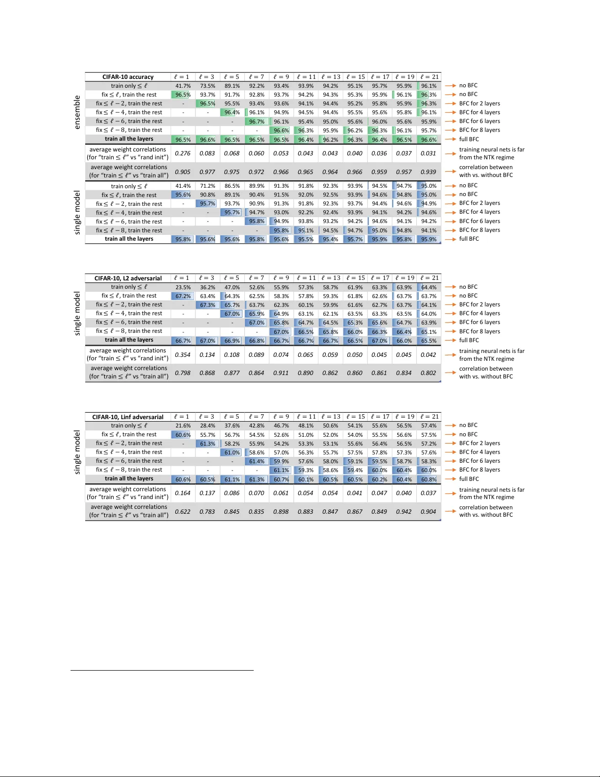
Bac kw ard F eature Correction: Ho w Deep Learning P erforms Deep (Hierarc hical) Learning Zeyuan Allen-Zh u zeyuanallenzhu@meta.com Meta F AIR Labs Y uanzhi Li Yuanzhi.Li@mbzuai.ac.ae Mohamed bin Za yed Univ ersit y of AI Jan 13, 2020 (v ersion 6) ∗ Abstract Deep learning is also kno wn as hierarchical learning, where the learner le arns to represent a complicated target function b y decomp osing it in to a sequence of simpler functions to reduce sample and time complexit y. This pap er formally analyzes ho w m ulti-la yer neural netw orks can p erform suc h hierarc hical learning eﬃciently and automatic al ly by applying stochastic gradien t descen t (SGD) or its v arian ts on the training ob jective. On the conceptual side, w e presen t a theoretical characterizations of how certain types of deep (i.e. sup er-constantly man y lay ers) neural net w orks can still b e sample and time eﬃcien tly trained on some hierarchical learning tasks, when no existing algorithm (including lay erwise training, k ernel metho d, etc) is kno wn to b e eﬃcient. W e establish a new principle called “bac kward feature correction”, where the err ors in the lower-level fe atur es c an b e automatic al ly c orr e cte d when tr aining to gether with the higher-level layers . W e b eliev e this is a key b ehind ho w deep learning is p erforming deep (hierarchical) learning, as opp osed to lay erwise learning or simulating some kno wn non-hierarchical method. On the technical side, we show for every input dimension d > 0, there is a concept class of degree ω (1) m ulti-v ariate p olynomials so that, using ω (1)-lay er neural netw orks as learners, a v ariant of SGD can learn an y function from this class in poly ( d ) time to an y 1 poly ( d ) error, through learning to represent it as a comp osition of ω (1) lay ers of quadratic functions using “backw ard feature correction”. In con trast, w e do not kno w an y other simpler algorithm (including la yerwise training, applying kernel metho d sequentially, training a tw o-lay er netw ork, etc) that can learn this concept class in p oly ( d ) time even to an y d − 0 . 01 error. As a side result, we pro ve d ω (1) lo wer b ounds for several non-hierarchical learners, including any kernel metho ds, neural tangent or neural comp ositional k ernels. ∗ V1 app ears on this date, V2 adds more exp erimen ts, V3 p olishes writing and improv es exp erimen ts, V4 makes minor ﬁxes to the ﬁgures, V5/V6 polish writing. V6 is accepted for presen tation at the Conference on Learning Theory (COL T) 2023. W e would like to thank, in chronological order, Sanjeev Arora, S ´ ebastien Bub ec k, James R. Lee, Edouard Oyallon, Elc hanan Mossel, Ruosong W ang for man y suggestions on this pap er. The most recent presen tations of this pap er can b e found at https://youtu.be/sd2o1PbqixI (by Z.A.) and at https://youtu.be/N8WIplddCuc (b y Y.L.). Most of the w ork w as done when Z.A. was at Microsoft Researc h Redmond. 1 In tro duction Deep learning is also kno wn as hierarchical (feature) learning. 1 The term hierarchical learning can b e deﬁned as learning to represent the c omplex target function g ( x ) using a comp osition of much simpler functions: g ( x ) = h L ( h L − 1 ( · · · h 1 ( x ) · · · )). In deep learning, for example, eac h h ℓ ( · ) is usually a linear operator follo wed with a simple elemen t-wise non-linear function (called activ ation). Empirically, the training process of deep learning is done by sto chastic gradient descent (SGD) or its v ariants. After training, one can v erify that the complexity of the learned fe atur es (i.e., h ℓ ( h ℓ − 1 ( · · · x · · · )) indeed increases as ℓ go es deep er— see [79] or Figure 1. It has also b een dis- co vered for a long time that hierarchical learning, in many applications, requires few er training examples [18] when compared with non-hierarc hical metho ds that learn g ( x ) in one shot. l a y er 1 l a y er 3 l a y er 9 l a y er 11 l a y er 13 l a y er 21 l a y er 23 l a y er 27 l a y er 31 i np ut outpu t … l a y er 19 l a y er 17 l a y er 15 l a y er 25 l a y er 29 l a y er 5 l a y er 7 … … … … … … … … … … … … … … … Figure 1: Illustration of the hierarchical learning pro cess of ResNet-34 on CIF AR-10. Details see Section 8.1. Hierarc hical learning from a theoretical p ersp ectiv e. In tuitively, hierarchical learning can signiﬁcan tly reduce the diﬃcult y of learning a complicated target function in one shot to learning a sequence of m uch simpler functions in m ultiple steps. F or example, instead of learning a degree 2 L function from scratc h, hierarchical learning can learn to represent it as a composition of L -quadratic functions, and thus learning one quadratic function at a time. Moreov er, it is well-kno wn that neural net works can indeed r epr esent a wide range of complicated functions using the comp osition of m uch simpler la yers. Ho wev er, the main diﬃcult y here is that being able to r epr esent a complex target function in a hierarchical netw ork do es not necessarily guarantee eﬃcient learning. F or example, L la y ers of quadratic netw orks can eﬃciently represent all parit y functions up to degree 2 L ; but in the deep L = ω (1) setting, it is unclear if one can learn parit y functions ov er x ∈ {− 1 , 1 } d with noisy lab els via any eﬃcien t p oly ( d )-time algorithm [28], not to say via training neural netw orks. 2 So, for what type of functions can w e formally pr ove that deep neural netw orks can hierarchically learn them? And, how can deep learning perform hierarc hical learning to greatly improv e learning eﬃciency in these cases? Hierarc hical learning and lay erwise learning. Motiv ated b y the large b ody of theory w orks for tw o-lay er net works, a tentativ e approac h to analyze hierarchical learning in deep learning is via 1 Quoting Bengio [16], “deep learning metho ds aim at le arning fe ature hierar chies with features from higher levels of the hierarch y formed by the comp osition of lo wer level features.” Quoting Goo dfello w et al. [33] “the hierarch y of concepts allows the computer to learn complicated concepts by building them out of simpler ones .” 2 Note, neural net works in practice are very robust to label noise. 1 epoc h 1 epoc h 6 0 epoc h 8 0 epoc h 2 0 0 f or w a r d f ea t ur e l ea r ni ng ba ck w ar d f ea t ur e c or r ec t i on epoc h 1 0 0 … … … … 1 st la y er f ea t u r es n o lo n g er imp r ov e t h r ou gh t r ain in g on ly 1 st la y er 1 st la y er f ea t u r es imp r ov e a g a in on c e w e s t art t o also t r ain h igh er - le v el la y er s Figure 2: Conv olutional features of the ﬁrst lay er in AlexNet. In the ﬁrst 80 ep ochs, we train only the ﬁrst la yer freezing lay ers 2 ∼ 5; in the next 120 ep ochs, we train all the la yers together (starting from the weigh ts in ep och 80). Details in Section 8.2. F or visualizations of deep er layers of R esNet , see Figure 3 and 12. Observ ation : In the ﬁrst 80 ep ochs, when the ﬁrst lay er is trained until conv ergence, its features can already catch certain meaningful signals, but cannot get further improv ed. As so on as the 2nd through 5th lay ers are added to the training parameters, features of the ﬁrst lay er get improv ed again. la yerwise training. Consider the example of using a multi-la yer netw ork with quadratic activ ation, to learn the follo wing target function. g ( x ) = x 2 1 + 2 x 2 2 | {z } low-complexit y signal +0 . 1 ( x 2 1 + 2 x 2 2 + x 3 ) 2 | {z } high-complexity signal . (1.1) In this example, one may hop e for ﬁrst training a tw o-lay er quadratic netw ork to learn simple, quadratic features ( x 2 1 , x 2 2 ), and then training another tw o-lay er quadratic net work on top of the ﬁrst one learns a quadratic function ov er ( x 2 1 , x 2 2 , x 3 ). In this w ay, one can hop e for nev er needing to learn a degree-4 polynomial in one shot, but simply learning t wo quadratic functions in tw o steps. Is hierarc hical learning in deep learning really this simple? In fact, lay erwise training is known to p erform p o orly in practical deep learning, see Figure 7. The main reason is that when w e train low er-lev el lay ers, it migh t ov er-ﬁt to higher-lev el features. Using the example of (1.1), if one uses a quadratic netw ork to ﬁt g ( x ), then the ﬁrst-la yer features ma y b e trained too greedily and o ver-ﬁt to high-complexity signals: for instance, the b est quadratic net work to ﬁt g ( x ) may learn features ( x 1 + √ 0 . 1 x 3 ) 2 and x 2 2 , instead of ( x 2 1 , x 2 2 ). No w, if w e freeze the ﬁrst lay er and train a second la y er quadratic net work on top of it (and the input), this “error” of √ 0 . 1 x 3 can no longer b e ﬁxed thus w e cannot ﬁt the target function p erfectly. Our main message. On the conceptual lev el, w e show (b oth theoretically and empirically) although low er-level lay ers in a neural netw ork indeed tend to o v er-ﬁt to higher complexity signals at the b eginning of training, when training all the la yers together— using simple v ariants of SGD— the presence of higher-lev el lay ers can even tually help reduce this type of o ver-ﬁtting in lo wer- lev el la yers. F or example, in the ab o ve case the quality of low er-level features can improv e from ( x 1 + √ 0 . 1 x 3 ) 2 again to get closer and closer to x 2 1 when trained together with higher-lev el lay ers. W e call this b ackwar d fe atur e c orr e ction . More generally, we identify two critic al steps in the hierarc hical learning pro cess of a m ulti-lay er net work. • The forwar d fe atur e le arning step, where a higher-level la yer can learn its features using the simple combinations of the learned features from low er-level lay ers. This is an analog of la yerwise training, but a bit diﬀerent (see discussions in [3]) since all the lay ers are still trained simultane ously . 2 l a y er 1 3 acc 58 .6% (if on ly t r ain ≤ 13 la y er s) ac c 67 .0% ( if t r ain all la y er s t og e t h er) pe r - c ha nn el feat ur e b ac kw ar d f ea tu r e c or r ec tion acc 0.0 % (r an d om in it ) f or w ar d f ea tu r e learn ing Figure 3: Visualize backw ard feature correction using WRN-34-5 on ℓ 2 adversarial tr aining . Details in Section 8.5. Observ ation: if only training lo wer-lev el la yers of a neural netw ork, the features ov er-ﬁt to higher- complexit y signals of the images; while if training all the lay ers together, the higher-complexity signals are learned on higher-level lay ers and shall b e “subtracted” from the low er-level features. This explains why layerwise tr aining is not a go o d choic e , and the mathematical intuitions can be found in Section 1.2. • The b ackwar d fe atur e c orr e ction step, where a low er-level lay er can learn to further impr ove its feature qualit y with the help of the learned features in higher-lev el la yers. W e are not a ware of this b eing recorded in the theory literature, and believe it is a most critic al r e ason for why hierarc hical learning go es b eyond lay erwise training in deep learning. W e shall mathematically c haracterize this in Theorem 2. R emark. When all the lay ers of a neural netw ork are trained together, the aforemen tioned t wo steps actually o ccur simultane ously . F or interested readers, w e also design exp erimen ts to separate them and visualize, see Figure 2, 3, and 12. On the theoretical side, we also giv e toy examples with mathematical in tuitions in Section 1.2 to further explain the tw o steps. Our technical results. With the help of the disco vered conceptual message, w e sho w the follo wing tec hnical results. Let input dimension d b e suﬃciently large, there exist a non-trivial class of “well- conditioned” L -la yer neural netw orks with L = ω (1) and quadratic activ ations 3 so that: • T raining such net works b y a v arian t of SGD eﬃciently and hier ar chic al ly learns this concept class. Here, by “eﬃciently” we mean time/sample complexit y is p oly ( d/ε ) where ε is the generalization error; and by “hierarchically” we mean the netw ork learns to represent the concept class b y decomp osing it into a comp osition of simple (i.e. quadratic) functions, via forw ard feature learning and backw ard feature correction, to signiﬁcantly reduce sample/time complexit y. • W e are una ware of existing algorithm that can ac hieve the same result in polynomial time. F or completeness, w e prov e sup er-polynomial low er b ounds for shallo w learning metho ds such as (1) k ernel metho d, (2) regression ov er feature mappings, (3) tw o-lay er netw orks with degree ≤ 2 L activ ations, or (4) the previous three with an y regularization. Although proving separation is 3 It is easy to measure the netw ork’s growing representation p ow er in depth using quadratic activ ations [57]. As a separate note, quadratic netw orks perform as w ell as ReLU netw orks in practice (see Figure 4 on P age 5), signiﬁcan tly b etter than (even ReLU net work’s) lay erwise learning, and has cryptographic adv antages [60]. 3 not our main message , 4 w e still illustrate in Section 1.2 that neither do we b eliev e lay erwise training, or applying kernel metho d multiple (even ω (1) man y) times can achiev e p oly-time. 5 T o this exten t, we hav e shown, at least for this class of L -la yer netw orks with L = ω (1), de ep le arning c an inde e d p erform eﬃcient hier ar chic al le arning when trained b y a v ariant of SGD to learn functions not known to be learnable by “shallo w learners” (including lay erwise training which can b e viewed as applying tw o-lay er netw orks m ultiple times). Thus, we b elieve that hierarchical learning (esp ecially with backw ard feature correction) is critic al to learn this concept class. Diﬀerence from existing theory. Man y prior and followup works hav e studied the theory of deep learning. W e try to cov er them all in Section 7 but summarize our main diﬀerence as follows. • Starting from Jacot et al. [42], there is a rich literature [3, 4, 6 – 8, 11, 12, 20, 21, 23, 25, 26, 32, 34, 39, 42, 48, 52, 62, 67, 76, 82, 83] that reduces multi-la yer neural net w orks to k ernel metho ds (e.g. neural tangent kernels, or NTKs). They approximate neural netw orks by line ar mo dels o ver (hierarc hically deﬁned) random features— which are not le arne d through training. They do not sho w the p o wer of deep learning b ey ond kernel methods. • Man y other theories [5, 13, 17, 19, 22, 30, 31, 44, 46, 47, 49 – 51, 64, 68, 69, 72, 74, 75, 77, 80, 81] fo cus on t wo-la yer netw orks but they do not hav e the de ep hier ar chic al structure. In particular, some ha ve studied fe atur e le arning as a pro cess [5, 22, 53], but still cannot co ver how the features of the second lay er can help backw ard correct the ﬁrst lay er; th us naively rep eating them for m ulti-lay er net works may only giv e rise to lay erwise training. • Allen-Zh u et al. [6] shows that 3-la yer neural netw orks can learn the so-called “second-order NTK,” which is not a linear mo del; how ever, second-order NTK is also learnable b y doing a n uclear-norm constrained linear regression, which is still not truly hierarc hical. • Allen-Zh u and Li [3] shows that 3-la yer ResNet can learn a concept class otherwise not learnable b y k ernel metho ds (within the same lev el of sample complexity). W e discuss more in Section 7, but most imp ortan tly, that concept class is learnable b y applying kernel method twice. In sum, most prior w orks ma y hav e only studied a simpler but already non-trivial question: “can m ulti-lay er neural netw orks eﬃciently learn simple functions that are also le arnable b y non- hierarc hical mo dels.” While the cited works shed great light on the learning pro cess of neural net works, in the language of this paper, they cannot justify ho w deep learning p erforms de ep hier ar chic al fe atur e le arning . Our work is motiv ated by this huge gap b et ween theory and practice. (W e also cite some works that study hierarchical learning in other con texts in Section 7.) Admittedly, with a more am bitious goal we ha ve to sacriﬁce something. Notably, we study quadratic activ ations which are conv entional in theory literature, but a few cited works ab o ve can handle ReLU. This ma y b e still ﬁne: in practice, deep learning with quadratic activ ations perform v ery closely to ReLU ones, signiﬁcan tly b etter than tw o-lay er net works or neural k ernel metho ds (see Figure 4), and muc h b etter than (even ReLU netw ork’s) la yerwise training (see Figure 7). Hence, our theoretical result ma y also serv e as a provisional step tow ards understating the deep learning pro cess in ReLU net works. In addition, as one shall see, we hav e slightly re-parameterized the netw ork, added regularizers, and made minor changes to the SGD algorithm to obtain our ﬁnal theoretical pro of. All of such may not appear conv en tional; but this may not b e to o bad, as in 4 Prior results suc h as [27, 70] separate the representation p o wer of multi-la yer netw orks from shallow er learners (without eﬃcient training guaran tee), and concurrent results [22, 53] separate the p o wer of two-layer neural net works from kernel metho ds with eﬃcient training guarantees. How ever, proving separation is not the main message of this pap er, and we fo cus on understanding how deep learning p erform eﬃcient hierarc hical learning when L = ω (1). 5 In contrast, prior work [3] can b e simulated by applying kernel metho d twice, see discussions in Section 7. 4 C IF A R - 10 ac c u r ac y C IF A R - 100 ac c u r ac y tr ai n i n g ti me H i e rar c h i c al l e arn i n g s i n g l e mo d e l e n s e m b l e s i n g l e mo d e l e n s e m b l e WRN - 16 - 10 96.27% 96.8% 80.28% 83.18% 2.5 G P U h o ur ( V100) WRN - 22 - 10 96.59% 97.12% 81.43% 84.33% 3 G P U h o ur ( V100) q u ad r ati c WRN - 16 - 10 94.68% 95.65% 75.31% 79.01% 3 G P U h o ur ( V100) q u ad r ati c WRN - 22 - 10 95.08% 95.97% 75.65% 79.97% 3.5 G P U h o ur ( V100) Ke rn e l me th o d s n e u ral c o mp o s i ti o n a l ke rn e l * w i th ZCA p r e p ro c e s s i n g 89.8% 89.8% 68.2% 68.2% ~ 1000 G P U h o ur n e u ral tan g e n t ke rn e l ( N T K) ** ( + r a n d o m p r ep r o ces si n g ) 81.40% 81.40% - - ~ 1000 G P U h o ur ( 88. 36 % ) - - - ~ 1000 G P U h o ur n e u ral G au s s i an p ro c e s s ke rn e l ** ( + r a n d o m p r ep r o ces si n g ) 82.20% 82.20% - - ~ 1000 G P U h o ur ( 88.92% ) - - - ~ 1000 G P U h o ur fin i te - w i d t h N T K fo r WR N - 10 - 10 ( + ZCA p r ep r o ces si n g ) 72.33 % 75.26% - - 20.5 G P U h o ur ( T i t an V ) ( 76.94 %) ( 80.21 %) - - 20.5 G P U h o ur ( T i t an V ) Figure 4: Comparison b et ween ReLU netw orks, quadratic netw orks, and several optimized kernel metho ds (* for [67] and ** for [54]). Details in Section 8.3. T ake-a wa y messages: Quadratic netw orks perform comparable to ReLU, and b etter and much faster than kernel metho ds. Finite-width NTK [8] accuracy is muc h w orse than its coun terparts in hierarchical learning, showing its insuﬃciency for understanding the ultimate p ow er of neural net works. Note 1: Kernel metho ds usually cannot b eneﬁt from ensemble since it is typically strictly con vex. Random preprocessing in principle may help if one runs it m ultiple times; but we exp ect the gain to be little. Ensem ble helps on ﬁnite-width NTK (linear function ov er random feature mappings) b ecause the feature space is re-randomized multiple times, so ensemble actually increases the n umber of features. Note 2: Our obtained accuracies using quadratic netw orks may b e of indep enden t interests: netw orks with quadratic activ ations ha ve certain practical adv antage esp ecially in cryptographic applications [60]. practice, when training neural netw orks for a hard dataset, one also needs to develop tons of hacks to mak e the training work. 1.1 Our Theorem W e give an ov erview of our theoretical result. The learner net works w e consider are DenseNets [38]: G ( x ) = P L ℓ =2  u ℓ , G ℓ ( x )  ∈ R where G 0 ( x ) = x ∈ R d , G 1 ( x ) = σ ( x ) − E [ σ ( x )] ∈ R d G ℓ ( x ) = σ  P j ∈J ℓ M ℓ,j G j ( x )  for ℓ ≥ 2 and J ℓ ⊆ { 0 , 1 , · · · , ℓ − 1 } (1.2) Here, σ is the activ ation function and we pick σ ( z ) = z 2 in this pap er, M ℓ,j ’s are w eight matrices, and the ﬁnal output G ( x ) ∈ R is a weigh ted summation of the outputs of all the la y ers. The set J ℓ deﬁnes the connection graph. W e can handle any connection graph with the only restriction b eing there is at least one “skip link.” 6 T o illustrate the main idea, we fo cus here on a regression problem in the teacher-studen t setting, although our result applies to classiﬁcation as well as the agnostic le arning setting (where the target netw ork ma y also hav e lab el error). In this teacher-studen t regression setting, the goal is to learn some unknown target function G ⋆ ( x ) in some concept class giv en samples ( x, G ⋆ ( x )) where x ∼ D follo ws some distribution D . In this pap er, w e consider the target functions G ⋆ ( x ) ∈ R coming from the same class as the learner netw ork: G ⋆ ( x ) = P L ℓ =2 α ℓ ·  u ⋆ ℓ , G ⋆ ℓ ( x )  ∈ R where G ⋆ 0 ( x ) = x ∈ R d , G ⋆ 1 ( x ) = σ ( x ) − E [ σ ( x )] ∈ R d G ⋆ ℓ ( x ) = σ  P j ∈J ℓ W ⋆ ℓ,j G ⋆ j ( x )  ∈ R k ℓ for ℓ ≥ 2 and J ℓ ⊆ { 0 , 1 , · · · , ℓ − 1 } (1.3) 6 In symbols, for every ℓ ≥ 3, w e require ( ℓ − 1) ∈ J ℓ , ( ℓ − 2) / ∈ J ℓ but j ∈ J ℓ for some j ≤ ℓ − 3. As comparisons, the v anilla feed-forward netw ork corresp onds to J ℓ = { ℓ − 1 } , while ResNet [36] (with skip connection) corresponds to J ℓ = { ℓ − 1 , ℓ − 3 } with w eight sharing (namely, M ℓ,ℓ − 1 = M ℓ,ℓ − 3 ). 5 Figure 5: Justiﬁcation of information gap on the CIF AR datasets for WRN-34-10 architecture. The 16 colors represen t 16 diﬀerent depths, and deep er lay ers hav e diminishing contributions to the classiﬁcation accuracy. W e discuss details in Section 3.2 and exp eriment details in Section 8.6. Since σ ( z ) is degree 2-homogenous, without loss of generality we assume ∥ W ⋆ ℓ,j ∥ 2 = O (1), u ⋆ ℓ ∈ {− 1 , 1 } k ℓ and let α ℓ ∈ R > 0 b e a scalar to control the con tribution of the ℓ -th lay er. In the teac her-student setting, our main theorems can b e sketc hed as follows: Theorem (sketc hed) . F or every input dimension d > 0 and every L = o (log log d ) , for c ertain c onc ept class c onsisting of c ertain L -layer tar get networks deﬁne d in Eq. (1.3), over c ertain input distributions (such as standar d Gaussian, c ertain mixtur e of Gaussians, etc.), we have: • Within p oly ( d/ε ) time/sample c omplexity, by a variant of SGD starting fr om r andom initializa- tion, the L -layer quadr atic DenseNet c an le arn this c onc ept class with any gener alization err or ε , using forw ard feature learning + bac kw ard feature correction . (Se e The or em 1.) • As side r esult, we show any kernel metho d, any line ar mo del over pr escrib e d fe atur e map- pings, or any two-layer neur al networks with arbitr ary de gr e e- 2 L activations, r e quir e d Ω(2 L ) sample or time c omplexity, to achieve non-trivial gener alization err or such as ε = d − 0 . 01 . (Se e Se ction H.) R emark. As w e shall formally introduce in Section 2, the concept class in our theorem— the class of target functions to b e learned— comes from Eq. (1.3) with additional width requiremen t k ℓ ≈ d 1 / 2 ℓ and information gap requiremen t α ℓ +1 ≪ α ℓ with α 2 = 1 and α L ≥ 1 √ d . The requirement L = o (log log d ) is very natural: a quadratic net work even with constant condition n um b er can output 2 2 L and w e need this to b e at most p oly ( d ) to pro ve an y eﬃcien t training result. W e refer the assumption α ℓ +1 ≪ α ℓ as information gap . In a classiﬁcation problem, it can b e understo od as “ α ℓ is the incremental accuracy impro vemen t when using ℓ -lay er netw orks to ﬁt the target comparing to ( ℓ − 1)-la yer ones.” W e discuss more in Section 3.2. F or example, in Figure 5, w e see > 75% of the CIF AR-10 images can b e classiﬁed correctly using a 2-lay er net work; but going from depth 7 to 8 only giv es < 1% accuracy gain. Information gap w as also p oin ted out in natural language pro cessing applications [71]. W e refer to [3] for empirical evidence that deep learning fails to p erform hierarchical learning when information gap is remo ved. 1.2 High-Lev el In tuitions In this subsection we included a “pro of by example”; later with all the notations introduced, w e ha ve a 4-paged sk etched pro of in Section 6 whic h shall mak e this “pro of by example” more concrete. In tuitively, learning a single quadratic function is easy, but our concept class consists of a suﬃcien tly ric h set of degree 2 L = 2 ω (1) p olynomials o ver d dimensions. Using non-hierarchical learning metho ds, typical sample/time complexity is d Ω(2 L ) = d ω (1) — and w e prov e such lo w er b ound for kernel (and some other) metho ds, even when all k ℓ = 1. This is not surprising , since 6 k ernel methods do not perform hierarc hical learning so hav e to essentially “write do wn” all the monomials of degree 2 L − 1 , whic h suﬀers a lot in the sample complexit y. Ev en if the learner p erforms k ernel metho d O (1) times, since the target function has width k ℓ = d Ω(1) for any constan t ℓ , this cannot av oid learning in one level a degree- ω (1) p olynomial that dep ends on d Ω(1) v ariables, resulting again in sample/time complexit y d ω (1) . No w, the hop e for training a quadratic DenseNet with p oly ( d ) time, is because it may decomp ose a degree-2 L p olynomial into learning one quadratic function at a time. Easier said than done, let us pro vide intuition by considering an extremely simpliﬁed example: L = 3, d = 4, and G ⋆ ( x ) = x 4 1 + x 4 2 + α (( x 4 1 + x 3 ) 2 + ( x 4 2 + x 4 ) 2 ) for some α = o (1). (Recall L = 3 refers to ha ving tw o trainable la yers that w e refer to as the second and third lay ers.) F orw ard feature learning: ric her represen tation b y o ver-parameterization. Since α ≪ 1, one ma y hop e for the second lay er G 2 ( x ) to learn x 4 1 and x 4 2 — whic h is quadratic ov er G 1 ( x )— through some represen tation of its neurons; then feed this as input to the third lay er. If so, the third lay er G 3 ( x ) could learn a quadratic function o ver x 4 1 , x 4 2 , x 3 , x 4 to ﬁt the remainder α (( x 4 1 + x 3 ) 2 + ( x 4 2 + x 4 ) 2 ) in the ob jective. This logic has a critical ﬂa w: • Inste ad of le arning x 4 1 , x 4 2 , the se c ond layer may as wel l le arn 1 5 ( x 2 1 + 2 x 2 2 ) 2 , 1 5 (2 x 2 1 − x 2 2 ) 2 . Indeed, 1 5 ( x 2 1 + 2 x 2 2 ) 2 + 1 5 (2 x 2 1 − x 2 2 ) 2 = x 4 1 + x 4 2 ; ho wev er, no quadratic function ov er 1 5 ( x 2 1 + 2 x 2 2 ) 2 , 1 5 (2 x 2 1 − x 2 2 ) 2 and x 3 , x 4 can pro duce ( x 4 1 + x 3 ) 2 + ( x 4 2 + x 4 ) 2 . Therefore, the second la yer needs to learn not only ho w to ﬁt x 4 1 + x 4 2 but also the “correct basis” x 4 1 , x 4 2 for the third la yer. T o achiev e this goal, w e let the learner net work to use (quadratically-sized) ov er-parameterization with random initialization. Instead of ha ving only tw o hidden neurons, we will let the net work ha ve m > 2 hidden neurons. W e show a critical lemma that the neurons in the second la yer of the net work can learn a richer r epr esentation of the same function x 4 1 + x 4 2 , giv en by: { ( α i x 2 1 + β i x 2 2 ) 2 } m i =1 In each hidden neuron, the co eﬃcien ts α i , β i b eha ve like i.i.d. Gaussians. Indeed, E [( α i x 2 1 + β i x 2 2 ) 2 ] ≈ x 4 1 + x 4 2 , and w.h.p. when m ≥ 3, we can sho w that a quadratic function of { ( α i x 2 1 + β i x 2 2 ) 2 } m i =1 , x 3 , x 4 can b e used to ﬁt ( x 4 1 + x 3 ) 2 + ( x 4 2 + x 4 ) 2 , so the algorithm can pro ceed. Note this is a completely diﬀerent view comparing to prior w orks: here ov er-parameterization is not to mak e training easier in the current lay er; instead, it enforces the netw ork to learn a richer set of hidden features (to represen t the same target function) that can b e b etter used for higher la yers. Bac kw ard feature correction: improv ement in lo wer lay ers after learning higher la yers. The second obstacle in this to y example is that the second la yer migh t not ev en learn the function x 4 1 + x 4 2 exactly . It is p ossible to come up with a distribution where the b est quadratic ov er G 1 ( x ) (i.e., x 2 1 , x 2 2 , x 2 3 , x 2 4 ) to ﬁt G ⋆ ( x ) is instead ( x 2 1 + αx 2 3 ) 2 + ( x 2 2 + αx 2 4 ) 2 , whic h is only of magnitude α close to the ideal function x 4 1 + x 4 2 . 7 This is over-ﬁtting , and the error αx 2 3 , αx 2 4 c annot b e corrected b y o ver-parameterization. (More generally, this error in the lo wer-lev el features can propagate lay er after lay er, if one keeps p erforming forward feature learning without going back to correct them. This why w e do not b eliev e applying kernel method sequentially ev en ω (1) times can p ossibly learn our concept class in p oly-time. W e discuss more in Section 3.) Let us proceed to see how this ov er-ﬁtting on the second la yer can b e corrected b y learning the third lay er together. Say the second la yer has an “ α -error” and feeds the o ver-ﬁt features 7 This additional error α is precisely b ecause there is a higher-complexity signal of magnitude α in the target function, which cannot b e ﬁt using the current lay er (since it exceeds degree 4 which is the maximum degree p olynomial w e can ﬁt using only the second lay er). 7 i nput l a y er 2 l a y er 3 l a y er 4 1 2 3 4 5 8 6 7 7 1) l a y er 2 b e g i n s t o l earn 2) l a y er 3 b e g i n s t o l earn us i ng f ea tur es giv en b y l a y er 2 3) l a y er 3 help s l a y er 2 c or r ect i ts f ea tur es b y r edu c i ng o v er - fit ti ng 4) l a y er 3 i mpr o v es s i nce la y er 2 no w f ee ds in be t t er f ea tur es t o l a y er 3 5) l a y er 4 b e g i n s t o l earn 6) l a y er 4 he l p s l a y er 2 c orr ect i ts f ea tur es b y r ed uci ng o v er - fit ti ng 7) l a y er 3 i mpr o v es s i nce a) l a y er 4 he l p s l a y er 3 c orr ect i ts f ea tur es b y r ed uci ng o v er - fit ti ng , an d b) l a y er 2 no w f ee ds in be t t er f ea tur es t o l a y er 3 8) l a y er 4 i mpr o v es s i nce la y er 3 no w f ee ds in be t t er f ea tur es Figure 6: Explain the hierarchical learning pro cess in a 4-lay er example. Bac k and blue arrows corresp ond to “forw ard feature learning” [3]; Red dashed arrows corresp ond to “backw ard feature correction” . Note: In our work, we do not explicitly tr ain the network in this or der, this “b ack and forth” le arning pr oc ess happ ens r ather implicitly when we simply tr ain al l layers in the network to gether . ( x 2 1 + αx 2 3 ) 2 , ( x 2 2 + αx 2 4 ) 2 to the third la yer. The third la yer can therefore use ∆ ′ = α (( x 2 1 + αx 2 3 ) 2 + x 3 ) 2 + α (( x 2 2 + αx 2 4 ) 2 + x 4 ) 2 to ﬁt the remainder term ∆ = α (( x 4 1 + x 3 ) 2 + ( x 4 2 + x 4 ) 2 ) in G ⋆ ( x ). A very neat observ ation is that ∆ ′ is only of magnitude α 2 a wa y from ∆. Therefore, when the second and third la yers are trained together, this “ α 2 -error” remainder ∆ ′ will b e subtracted from the training ob jective, so the second lay er can learn up to accuracy α 2 , instead of α . In other w ords, the amoun t of ov er-ﬁtting is no w reduced from α to α 2 . W e call this “backw ard feature correction.” (This is also consistent with what w e discov er on ReLU netw orks in real-life exp erimen ts, see Figure 3 where w e visualize such “ov er-ﬁtting.”) In fact, this pro cess α → α 2 → α 3 → · · · keeps going and the second lay er can feed b etter and b etter features to the third lay er (forward learning), via the reduction of ov er-ﬁtting fr om the third la yer (via backw ard correction). W e can even tually learn G ⋆ to arbitrarily small error ε > 0. When there are more than tw o trainable lay ers, the pro cess is slightly more inv olved, and w e summarize this hier ar chic al learning pro cess in Figure 6. 8 Hierarc hical learning in deep learning go es b eyond la y erwise training. Our results also shed ligh ts on the following observ ation in practice: t ypically lay erwise training (i.e. train lay ers one by one starting from low er levels) 9 p erforms m uch worse than training all the lay ers together, see Figure 7. The fundamental reason is due to the missing piece of “backw ard feature correction.” F rom in tuitions to theory. Although the in tuitions do seem to generally apply in practice (see Figure 3 and man y more experiments in the appendix), to actually pr ove them, w e mak e mo diﬁcations to the SGD algorithm and add regularizations. After the notations are introduced, in Section 6, w e giv e a more detailed, 4-paged sketc hed proof to mak e this “pro of by example” more concrete. 8 Moreo ver, as a separate interest, according to our theorem, the improv ement of low er-level features is mainly due to the “subtraction” of the higher-lev el signals. This means during training, most of the “backw ard” eﬀort in a neural net work is from the “identit y link”. This is consisten t with empirical w orks [14, 63], while the authors observ e that in ResNet, the “backw ard” from hidden weigh ts can be detached during the training of multi-la yer neural netw orks (except only k eeping the identit y link) to achiev e comparable p erformance on standard data sets. 9 W e refer to layerwise tr aining as ﬁrst training the 1st hidden lay er by setting other lay ers to zero, and then training the 2nd lay er b y ﬁxing the 1st lay er and setting others to zero, and so on. Suc h algorithm is used in theoretical works such as [59]. There exist other works that use (deep) auxiliary net works to train the la yers of a neural net work one by one [15]; the authors of [15] also refer to their algorithm as lay erwise training; but in our language, such results are performing hierarchical learning due to the existence of auxiliary netw orks. 8 60 70 80 90 10 0 0 4 8 12 16 CI F A R - 10 T es t Accu r acy % # o f la y e r s v gg- 19- la y e rw i s e v gg- 19 v gg- 19- x2- l a y e rw is e v gg- 19- x2 v gg- 19- x4- l a y e rw is e v gg- 19- x4 30 40 50 60 70 80 0 4 8 12 16 CI F A R - 100 T e s t Accu r acy % # o f la y e r s v gg - 19 - lay e rw i s e v gg - 19 v gg - 19 - x2 - l a y e rw ise v gg - 19 - x2 v gg - 19 - x4 - l a y e rw ise v gg - 19 - x4 (a) V GG19+BatchNorm, accuracy at x-axis S indicates only the ﬁrst S con volutional lay ers are trained 60 70 80 90 10 0 0 4 8 12 16 CIF A R - 10 T es t Acc u r acy % # o f b lo ck s WRN - 34 - lay e rw is e WRN - 34 WRN - 34 - x4 - lay e rw is e WRN - 34 - x4 WRN - 34 - x8 - lay e rw is e WRN - 34 - x8 WRN - 34 - x1 6- lay e rw is e WRN - 34 - x1 6 35 45 55 65 75 85 0 4 8 12 16 CIF A R - 100 T e s t Acc u r acy % # o f b lo ck s WRN - 34 - lay e rw is e WRN - 34 WRN - 34 - x4 - lay e rw is e WRN - 34 - x4 WRN - 34 - x8 - lay e rw is e WRN - 34 - x8 WRN - 34 - x1 6- lay e rw is e WRN - 34 - x1 6 (b) WideResNet-34, accuracy at x-axis S indicates only the ﬁrst S conv olutional blo c ks are trained Figure 7: Lay erwise training vs T raining all lay ers together. Details and more experiments in Section 8.4. T ake-a wa y messages: In lay erwise training, low er lay ers are trained to o greedily and ov er-ﬁt to higher- complexit y signals, leading to worse accuracy than hierarchical learning (i.e., training all the lay ers together), even at the se cond hidden layer . Going deep er cannot increase accuracy anymore as the lo w-quality features at low er la yers are already ﬁxed. F or moderately wide (e.g. width =64) architectures, la yerwise training stops improving test accuracy even after depth 3 without Backwar d F e atur e Corr e ction . 2 T arget Net work and Learner Net w ork T arget netw ork. W e consider a tar get network deﬁned as G ⋆ 0 ( x ) = x ∈ R d , G ⋆ 1 ( x ) = σ ( x ) − E [ σ ( x )] ∈ R d , G ⋆ ℓ ( x ) = σ  P j ∈J ℓ W ⋆ ℓ,j G ⋆ j ( x )  ∈ R k ℓ ∀ ℓ ≥ 2 where the w eight matrices W ⋆ ℓ,j ∈ R k ℓ × k j for ev ery ℓ, j . Each index set J ℓ is a subset of { 0 , 1 , 2 , · · · , ℓ − 3 } ∪ { ℓ − 1 } . W e assume that (1) ℓ − 1 ∈ J ℓ (so there is a connection to the immediate previous la yer) and (2) for ev ery ℓ ≥ 3, |J ℓ | ≥ 2 (so there is at least one skip connection). W e use the con ven tion W ⋆ ℓ,j = 0 if j / ∈ J ℓ . Our concept class to b e learned consists of functions G ⋆ : R d → R written as co ordinate sum- mation of eac h lay er: 10 G ⋆ ( x ) = P L ℓ =2 α ℓ · Sum ( G ⋆ ℓ ( x )) def = P L ℓ =2 α ℓ P i ∈ [ k ℓ ] G ⋆ ℓ,i ( x ) where Sum ( v ) def = 1 ⊤ v = P i v i , and it satisﬁes α 2 = 1 and α ℓ +1 < α ℓ . W e will pro vide more explanation of the meaningfulness and necessit y of information-gap α ℓ +1 < α ℓ in Section 3.2. It is con venien t to deﬁne S ⋆ ℓ ( x ) as the hidden fe atur es of target net work (and G ⋆ ℓ ( x ) = σ ( S ⋆ ℓ ( x ))). S ⋆ 0 ( x ) = G ⋆ 0 ( x ) = x, S ⋆ 1 ( x ) = G ⋆ 1 ( x ) , S ⋆ ℓ ( x ) def = P ℓ − 1 j =0 W ⋆ ℓ,j G ⋆ j ( x ) ∀ ℓ ≥ 2 Note for ℓ ≥ 2, S ⋆ ℓ ( x ) is of degree 2 ℓ − 1 and G ⋆ ℓ ( x ) = σ ( S ⋆ ℓ ( x )) is of degree 2 ℓ . Learner netw ork. Our goal is to construct a learner net w ork G of the same structure (with 10 Our result trivially extends to the case when Sum ( v ) is replaced with P i p i v i where p i ∈ {± 1 } for half of the indices. W e refrain from proving that v ersion for notational simplicity. 9 𝑆 0 𝑆 1 𝑆 2 𝑆 3 𝑆 4 𝑆 4 𝑆 ℓ − 2 𝑆 ℓ − 1 𝐹 ℓ = 𝜎 𝑊 ℓ , 1 ∎ + 𝑊 ℓ , 4 ∎ + 𝑊 ℓ , ℓ − 1 ∎ 𝑆 0 𝑆 1 𝑆 2 𝑆 3 𝑆 4 𝑆 4 𝑆 ℓ − 2 𝑆 ℓ − 1 𝑆 ℓ = 𝐾 ℓ , 1 ∎ + 𝐾 ℓ , 4 ∎ + 𝐾 ℓ , ℓ − 1 ∎ d is tilla tion 𝑊 ℓ , 1 𝑊 ℓ , 4 𝑊 ℓ , ℓ − 1 𝐾 ℓ , ℓ − 1 𝐾 ℓ , 4 𝐾 ℓ , 1 … … d is tilla tion d is tilla tion d is tilla tion Figure 8: learner netw ork structure with distillation o ver-parameterization) to simulate G ⋆ : G ℓ ( x ) = σ  P j ∈J ℓ M ℓ,j G j ( x )  . Here, G 0 ( x ) = x, G 1 = G ⋆ 1 ( x ) and we c ho ose M ℓ, 0 , M ℓ, 1 ∈ R ( k ℓ +1 2 ) × d and M ℓ,j ∈ R ( k ℓ +1 2 ) × ( k j +1 2 ) for ev ery 2 ≤ j ≤ ℓ − 1. In other w ords, the amoun t of ov er-parameterization is quadratic (i.e., from k j →  k j +1 2  ) p er lay er. W e wan t to construct the w eight matrices so that G ( x ) = P L ℓ =2 α ℓ Sum ( G ℓ ( x )) ≈ G ⋆ ( x ) . 2.1 Learner Net w ork Re-parameterization In this pap er, for theoretical eﬃcien t training purp ose, we work on a re-parameterization of the learner net work. W e use the following function to ﬁt the target G ⋆ ( x ): F ( x ) = P L ℓ =2 α ℓ · Sum ( F ℓ ( x )) where the la yers are deﬁned as: S 0 ( x ) = G ⋆ 0 ( x ), S 1 ( x ) = G ⋆ 1 ( x ), and for ℓ ≥ 2: 11 S ℓ ( x ) = P j ∈J ℓ ,j ≥ 2 K ℓ,j σ ( R j S j ( x )) + P j ∈{ 0 , 1 }∩J ℓ K ℓ,j S j ( x ) ∈ R k ℓ (2.1) F ℓ ( x ) = σ  P j ∈J ℓ ,j ≥ 2 W ℓ,j σ ( R j S j ( x )) + P j ∈{ 0 , 1 }∩J ℓ W ℓ,j S j ( x )  ∈ R m (2.2) Ab o ve, w e shall choose m to b e p olynomially large and let • R ℓ ∈ R ( k ℓ +1 2 ) × k ℓ b e randomly initialized for every la yer ℓ , not changed during training; and • W ℓ,j ∈ R m × q , K ℓ,j ∈ R k ℓ × q b e trainable for ev ery ℓ and j ∈ J ℓ , and the dimension q =  k j +1 2  for j ≥ 2 and q = d for j = 0 , 1. It is easy to v erify that when R ⊤ ℓ R ℓ = I and when W ℓ,j = K ℓ,j , by deﬁning M ℓ,j = R ℓ K ℓ,j w e hav e F ℓ ( x ) = G ℓ ( x ) and F ( x ) = G ( x ). W e remark that the hidden dimension k ℓ can also b e learned during training, see Algorithm 1 in Section 4. 12 Wh y this re-parameterization. W e work with this re-parameterization F ( x ) for eﬃcient tr ain- ing purp ose . It is con venien t to think of S ℓ ( x ) as the “ hidden fe atur es ” used by the learner net w ork. 11 Recall G ⋆ 1 ( x ) = σ ( x ) − E [ σ ( x )] and during training w e only hav e access to the empirical exp ectation of E [ σ ( x )]; ho wev er using p oly ( d/ε ) samples, the empirical expectation would b e 1 poly ( d/ε ) accurate. F or cleanness, we just write in S 1 the true expectation, we the diﬀerence can be easily dealt b y a Lipschitz argumen t (see Section C.3). 12 F rom this deﬁnition, it seems the learner needs to kno w { α ℓ } ℓ and {J ℓ } ℓ ; as we p oin t out in Section 4, p erforming grid search o ver them is eﬃcient in poly ( d ) time. This can b e viewed as neural architecture searc h. As a consequence, in the agnostic setting, our theorem can be understo od as: “the le arner network c an ﬁt the lab eling function using the b est G ⋆ fr om the c onc ept class as wel l as the b est choic es of { α ℓ } ℓ and {J ℓ } ℓ .” 10 Since S ℓ ( x ) is of the same dimension k ℓ as S ⋆ ℓ ( x ), our goal becomes to pro ve that the hidden features S ℓ ( x ) and S ⋆ ℓ ( x ) are close up to unitary transformation (i.e. Theorem 2). T o achiev e this, we consider an o ver-parameterized F ℓ ( x ) = σ ( W · · · ) and treat the pre- activ ation part ( W · · · ) ∈ R m in (2.2) as the “ov er-parameterized hidden features” o ver S ℓ ( x ) ∈ R k ℓ , for some m ≫ k ℓ . This ov er-parameterization is used to make training pr ovably eﬃcient , for a sim- ilar reason as [6]. W e shall imp ose regularizers to enforce K ⊤ K ≈ W ⊤ W whic h shall then make the hidden features S ℓ ( x ) also learned accurately . This idea of using a larger W for training and a smaller K to learn W can b e reminiscent of know le dge distil lation [37], and w e illustrate this b y Figure 8. In our sk etched-proof Section 6 (Page 23), w e giv e more details on this. 𝐵 ℓ ′ − 𝐵 ℓ ′ 0 i den t i c al t o 𝜎 𝑧 = 𝑧 2 f or some suffi cien t l y l ar g e 𝐵 ℓ ′ boun ded i n t he li mit … Figure 9: truncated quadratic activ ation T runcated quadratic activ ation. T o make our theory simpler, during tr aining , it w ould b e easier to work with an activ ation that has b ounded deriv a- tiv es in the en tire space (recall | σ ′ ( z ) | = | z | is un- b ounded). W e mak e a theoretical choice of a truncated quadratic activ ation e σ ( z ) that is suﬃcien tly close to σ ( z ). Accordingly , we rewrite F ( x ), F ℓ ( x ), S ℓ ( x ) as e F ( x ) , e F ℓ ( x ) , e S ℓ ( x ) whenev er we replace σ ( · ) with e σ ( · ). (F or completeness w e include the formal deﬁnition in App endix A.1.) Our lemma— see App endix C.1 — shall ensure that F ( x ) ≈ e F ( x ) and S ℓ ( x ) ≈ e S ℓ ( x ). Th us, our ﬁnal le arne d network F ( x ) is stil l of truly quadr atic activations . In practice, p eople use batc h/lay er normalizations to mak e sure activ ations sta y b ounded, but truncation is more theory-friendly. Notation simpliﬁcation. W e concatenate the weigh t matrices used in the same la y er ℓ as follo ws: W ℓ = ( W ℓ,j ) j ∈J ℓ K ℓ = ( K ℓ,j ) j ∈J ℓ W ⋆ ℓ =  W ⋆ ℓ,j  j ∈J ℓ W ℓ ◁ = ( W ℓ,j ) j ∈J ℓ ,j  = ℓ − 1 K ℓ ◁ = ( K ℓ,j ) j ∈J ℓ ,j  = ℓ − 1 W ⋆ ℓ ◁ =  W ⋆ ℓ,j  j ∈J ℓ ,j  = ℓ − 1 2.2 T raining Ob jective W e fo cus our notation for the regression problem in the realizable case. W e will in tro duce notations for the agnostic case and for classiﬁcation in Section 3.2 when we need them. As men tioned earlier, to p erform knowledge distillation, w e add a regularizer to ensure W ⊤ ℓ W ℓ ≈ K ⊤ ℓ K ℓ so that K ⊤ ℓ K ℓ is a low-rank appro ximation of W ⊤ ℓ W ℓ . (This also implies Sum ( F ℓ ( x )) ≈ Sum ( σ ( S ℓ ( x ))).) Sp eciﬁcally , w e use the following training ob jective: g Ob j ( x ; W , K ) = ] Loss ( x ; W , K ) + Reg ( W , K ) where the ℓ 2 loss is ] Loss ( x ; W , K ) = ( G ⋆ ( x ) − e F ( x )) 2 and Reg ( W , K ) = P L ℓ =2 λ 3 ,ℓ    K ⊤ ℓ,ℓ − 1 K ℓ ◁ − W ⊤ ℓ,ℓ − 1 W ℓ ◁    2 F + P L ℓ =2 λ 4 ,ℓ    K ⊤ ℓ,ℓ − 1 K ℓ,ℓ − 1 − W ⊤ ℓ,ℓ − 1 W ℓ,ℓ − 1    2 F + P L ℓ =2 λ 5 ,ℓ   K ⊤ ℓ K ℓ − W ⊤ ℓ W ℓ   2 F + P L ℓ =2 λ 6 ,ℓ  ∥ K ℓ ∥ 2 F + ∥ W ℓ ∥ 2 F  . F or a given set Z consisting of N i.i.d. samples from the true distribution D , the tr aining pr o c ess minimizes the follo wing ob jectiv e ( x ∼ Z denotes x is uniformly sampled from the training set Z ) g Ob j ( Z ; W , K ) = E x ∼Z [ g Ob j ( x ; W , K )] (2.3) 11 The regularizers we used are just (squared) F rob enius norm on the weigh t matrices, which are common in practice. The regularizers asso ciated with λ 3 ,ℓ , λ 4 ,ℓ , λ 5 ,ℓ are for know le dge distil lation pr op ose to mak e sure K is close to W (they are simply zero when K ⊤ ℓ K ℓ = W ⊤ ℓ W ℓ ). They play no r ole in backw ard feature corrections (since lay ers ℓ and ℓ ′ for ℓ ′  = ℓ are optimized indep endently in these regularizers). These corrections are done solely b y SGD automatically. F or the original, non-truncated quadratic activ ation netw ork, w e also denote by Loss ( x ; W , K ) = ( G ⋆ ( x ) − F ( x )) 2 and Ob j ( x ; W , K ) = Loss ( x ; W , K ) + Reg ( W , K ). 3 Statemen ts of Main Result W e assume the input distribution x ∼ D satisﬁes random prop erties suc h as isotropy and hyper- con tractivity. W e defer the details to Section 5, while pointing out that not only standard Gaussian but even some mixtures of non-spherical Gaussians satisfy these prop erties (see Prop osition 5.1). F or simplicity, the readers can think of D = N (0 , I ) in this section. W e consider a concept class consisting of target netw orks satisfying the following parameters 1. (monotone) d ≥ k def = k 2 ≥ k 3 ≥ · · · ≥ k L . 2. (normalized) E x ∼D [ Sum ( G ⋆ ℓ ( x ))] ≤ B ℓ for some B ℓ ≥ 1 for all ℓ and B def = max ℓ { B ℓ } . 3. (w ell-conditioned) the singular v alues of W ⋆ ℓ,j are b et ween 1 κ and κ for all ℓ, j ∈ J ℓ pairs. R emark 3.1 . Properties 1 , 3 are satisﬁed for many practical net w orks; in fact, man y practical net works hav e w eight matrices close to unitary, see [40]. F or prop ert y 2, although there may exist some worst case W ⋆ ℓ,j , at least when eac h W ⋆ ℓ,j is of the form U ℓ,j ΣV ℓ,j for U ℓ,j , V ℓ,j b eing random orthonormal matrices, with probabilit y at least 0 . 9999, it holds B ℓ = κ 2 O ( ℓ ) k ℓ for instance for standard Gaussian inputs— this is small since L ≤ o (log log d ). 13 Another view is that practical net works are equipp ed with batch/la yer normalizations, whic h ensure that B ℓ = O ( k ℓ ). Our results. In the main b o dy of this pap er, w e state a simple v ersion of our main (p ositiv e result) Theorem 1 which is suﬃciently in teresting. In App endix A, w e give a more general Theorem 1’ that includes more parameter regimes. In this simple v ersion, we assume there are absolute in teger constan ts C > C 1 ≥ 2 suc h that, the concept class consists of target netw orks G ⋆ ( x ) satisﬁes the ab o v e three prop erties with parameters κ ≤ 2 C L 1 , B ℓ ≤ 2 C ℓ 1 k ℓ , k ℓ ≤ d 1 C ℓ + C 1 and there is an information gap α ℓ +1 α ℓ ≤ d − 1 C ℓ for ℓ ≥ 2; furthermore, supp ose in the connection graph { 2 , 3 , · · · , ℓ − C 1 } ∩ J ℓ = ∅ , meaning that the skip connections do not go v ery deep, unless directly connected to the input. Theorem 1 (sp ecial case of Theorem 1’) . In the p ar ameter r e gime deﬁne d ab ove, for every suf- ﬁciently lar ge d > 0 , every L = o (log log d ) , every ε ∈ (0 , 1) , c onsider any tar get network G ⋆ ( x ) satisfying the ab ove p ar ameters. Then, given N = p oly ( d/ε ) i.i.d. samples x fr om D with c or- r esp onding lab els G ⋆ ( x ) , by applying A lgorithm 1 (a variant of SGD) with over-p ar ameterization m = p oly ( d/ε ) and le arning r ate η = 1 poly ( d/ε ) over the tr aining obje ctive (2.3), w ith pr ob ability at le ast 0.99, we c an ﬁnd a le arner network F in time p oly ( d/ε ) such that: E x ∼D  G ⋆ ( x ) − F ( x )  2 ≤ ε 2 and E x ∼D  G ⋆ ( x ) − e F ( x )  2 ≤ ε 2 . 13 In fact B ℓ = κ 2 O ( ℓ ) k ℓ holds as long as E  1 d ∥ x ∥ 2 2  2 ℓ  ≤ 2 2 O ( ℓ ) . This can b e deriv ed using E W ⋆ E x [ Sum ( G ⋆ ℓ ( x ))] = E x E W ⋆ [ Sum ( G ⋆ ℓ ( x ))], and it suﬃces to consider a ﬁxed x and use the randomness of W ⋆ to prov e the claim. 12 W e defer the detailed pseudo code 14 of Algorithm 1 to Section 4 but mak e several remarks: • Note α ℓ +1 = α ℓ d − 1 C ℓ implies α L ≥ d − 1 C ≥ 1 √ d is not small. Hence, to achiev e for instance ε ≤ 1 d 4 error, the learning algorithm has to truly learn al l the lay ers of G ⋆ ( x ), as opp osed to for instance ignoring the last lay er which will incur error α L ≫ ε . (W e choose this concept class so that learning all the la yers is necessary.) • The reason we fo cus on L = o (log log d ) and w ell-conditioned target netw orks should b e natural. Since the target net work is of degree 2 L , we wish to hav e κ 2 L ≤ p oly ( d ) so the output of the net work is b ounded by p oly ( d ) for eﬃcient learning. The main conceptual and tec hnical con tribution of our pap er is the “backw ard feature correction” pro cess. T o illustrate this, we highlight a critical lemma in our pro of and state it as a theorem: Bac kw ard F eature Correction Theorem Theorem 2 (highlight of Corollary E.3d) . In the setting of The or em 1, during the tr aining pr o- c ess, supp ose the ﬁrst ℓ -layers of the le arner network has achieved ε gener alization err or, or in symb ols, E  G ⋆ ( x ) − P ℓ ′ ≤ ℓ α ℓ ′ Sum ( F ℓ ′ ( x ))  2  ≤ ε 2 , (3.1) then for every ℓ ′ ≤ ℓ , ther e is unitary matrix U ℓ ′ ∈ R k ℓ ′ × k ℓ ′ such that (we write α L +1 = 0 ) E h α 2 ℓ ′ ∥ S ⋆ ℓ ′ ( x ) − U ℓ ′ S ℓ ′ ( x ) ∥ 2 i ≲ ( α 2 ℓ +1 + ε 2 ) . In other words, once we hav e trained the ﬁrst ℓ lay ers w ell enough, for some low er-level lay er ℓ ′ ≤ ℓ , the “error in the learned features S ℓ ′ ( x ) comparing to S ⋆ ℓ ′ ( x )” is pr op ortional to α ℓ +1 . Recall α ℓ is a decreasing sequence, th us Theorem 2 suggests that the lower-level fe atur es c an actual ly get impr ove d when we tr ain higher-level layers to gether. R emark 3.2 . Theorem 2 is not a “represen tation” theorem. There might b e other netw orks F suc h that (3.1) is satisﬁed but S ℓ ′ ( x ) is not close to S ⋆ ℓ ′ ( x ) at all. Theorem 2 implies during the tr aining pr o c ess , as long as we following carefully the training pro cess of SGD, suc h “bad F ” will b e automatically av oided. W e give more details in our in tuition and sketc hed pro of Section 6. Comparing to sequen tial kernel metho ds. Recall we hav e argued in Section 1.2 that our concept class is not lik ely to be eﬃcien tly learnable, if one applies kernel metho d O (1) times sequen tially. Ev en if one applies k ernel metho d for ω (1) rounds, this is similar to layerwise tr aining and misses “backw ard feature correction.” As we p oin ted out using examples in Section 1.2, this is unlik ely to learn the target function to go o d accuracy either. In fact, one ma y consider “sequential k ernel” together with “bac kw ard feature correction”, but even this may not alw ays work, since small generalization error do es not necessarily imply suﬃcient accuracy on in termediate features if we do not fol low the SGD tr aining pr o c ess (see Remark 3.2). 15 14 Algorithm 1. W e made mo diﬁcations on SGD to tradeoﬀ for easier pro ofs. Tw o noticeable diﬀerences are as follo ws. First, we start parameter training in the lay er order— train W 2 ﬁrst, then train W 2 , K 2 together, then train W 2 , K 2 , W 3 together, then train W 2 , K 2 , W 3 , K 3 together, etc. This is known as “lay erwise pretraining” which p erforms no w orse than “training all the lay ers together” and signiﬁcantly b etter than “lay erwise training.” Second, whenev er K ℓ is added to training, we let it start from an SVD w arm-start computed from W ℓ (done only once for eac h K ℓ ). Using SVD warm-start is a standard theory tec hnique in non-conv ex literature (at least tracing back to [10]), and it av oids the messier (and perhaps less interesting) pro ofs to deal with singularities in K ℓ . 15 One ma y also wan t to connect this to [3]: according to F o otnote 27, the analysis from [3] is analogous to doing “sequen tial kernel” for 2 rounds, but even if one wan ts to backw ard correct the features of the ﬁrst hidden lay er, its error remains to b e α and cannot b e improv ed to arbitrarily small. 13 Imp ortance of Hierarchical Learning: T o learn this concept class, to the b est of our kno wl- edge, • W e do not kno w an y other simple algorithm that can learn the target functions considered in this pap er within the same eﬃciency, the only simple learning algorithm we are a ware of is to train a neural net work to p erform hierarchical learning. • W e present a setting where w e can prov e that training a neural net w ork via a simple v ariant SGD can p erform hierarchical learning to solve an underlying problem that is not known solv able b y existing algorithms, such as applying kernel methods sequentially m ultiple times, tensor decomp osition metho ds, sparse co ding. Th us, neural net work has a unique learning mec hanism that is not sim ulating kno wn (non-hierarc hical) algorithms or their simple comp ositions . This can b e viewed as an evidence of why practitioners c ho ose to use neural net work instead of other metho ds in mo dern mac hine learning. Agnostic learning. Our theorem also works in the agnostic setting, where the lab eling function Y ( x ) satisﬁes E x ∼D ( G ⋆ ( x ) − Y ( x )) 2 ≤ OPT and | G ⋆ ( x ) − Y ( x ) | ≤ p oly ( d ) for some unknown G ⋆ ( x ). The SGD algorithm can learn a function F ( x ) with error at most (1 + γ ) OPT + ε 2 for any constant γ > 1 given i.i.d. samples of { x, Y ( x ) } . Th us, the learner can c omp ete with the performance of the b est target netw ork. W e present the result in App endix A.5 and state its sp ecial case b elo w. Theorem 3 (sp ecial case of Theorem 3’) . F or every c onstant γ > 0 , in th e same setting The or em 1, given N = p oly ( d/ε ) i.i.d. samples Z fr om D and their c orr esp onding lab els { Y ( x ) } x ∈Z , by apply- ing Algorithm 1 (a variant of SGD) over the agnostic tr aining obje ctive E x ∼Z  Y ( x ) − e F ( x )  2 + Reg ( W , K ) , with pr ob ability ≥ 0 . 99 , it ﬁnds a le arner network F in time p oly ( d/ε ) s.t. E x ∼D ( F ( x ) − Y ( x ))) 2 ≤ ε 2 + (1 + γ ) OPT . 3.1 Bac kw ard F eature Correction: How deep? How m uch? Ho w deep do es it need for the neural net w ork to p erform bac kw ard feature correction? In our theoretical result, we studied an extreme case in which training the L -th lay er can even bac kward correct the learned w eigh ts on the ﬁrst lay er for L = ω (1) (see Theorem 2). In practice, we demon- strate that backw ard feature correction ma y indeed need to be deep. F or the 34-la y er WideResNet arc hitecture on CIF AR tasks, see Figure 10 on Page 15, w e show that bac kward feature correction happ ens for at le ast 8 layers , meaning that if we ﬁrst train all the ≤ ℓ la yers for some large ℓ (sa y ℓ = 21), the features in lay er ℓ − 8 , ℓ − 7 , · · · , ℓ stil l ne e d to b e (lo c al ly) impr ove d in order to b ecome the b est features comparing to training all the lay ers together. This ﬁnding is consis ten t with [15] where the authors sho wed deep er “backw ard” during training leads to higher test accuracy . W e also giv e a characterization on ho w m uch the features need to b e bac kw ard corrected using theory and exp erimen ts. On the empirical side, we measure the changes given b y backw ard feature correction in Figure 10 and 11. W e detect that these changes are lo c al : meaning although the low er la yers need to c hange when training with higher lay ers together to obtain the highest accuracy, they do not change by much (the correlation of la yer weigh ts before and after backw ard correction is more than 0.9). In Figure 12, we also visualize the neurons at diﬀerent lay ers, so that one can easily see bac kward feature correction is indeed a lo c al c orr e ction pr o c ess in pr actic e . This is consisten t with our theory. Theorem 2 sho ws at least for our concept class, backw ard feature correction is a lo cal correction, meaning that the amoun t of feature c hange to the lo w er-level la yers (when trained together with higher-level la yers) is only little- o (1) due to α ℓ +1 ≪ α ℓ ′ . 14 C I F A R - 1 0 0 a c c u r a c y C o l u m n 1 C o l u m n 2 C o l u m n 3 C o l u m n 4 C o l u m n 5 C o l u m n 6 C o l u m n 7 C o l u m n 8 C o l u m n 9 C o l u m n 1 0 C o l u m n 1 1 1 6 .0 % 4 3 .1 % 6 1 .5 % 6 7 .9 % 7 0 .7 % 7 1 .5 % 7 5 .9 % 7 8 .6 % 7 9 .8 % 8 0 .6 % 8 0 .9 % 8 3 .1 % 7 8 .9 % 7 8 .4 % 7 6 .9 % 7 5 .9 % 7 5 .6 % 7 7 .6 % 7 9 .6 % 8 0 .5 % 8 1 .0 % 8 1 .2 % - 8 3 .4 % 8 1 .5 % 7 9 .8 % 7 8 .4 % 7 7 .4 % 7 8 .7 % 8 0 .3 % 8 0 .7 % 8 1 .0 % 8 1 .3 % - - 8 3 .1 % 8 1 .9 % 8 1 .2 % 8 0 .1 % 8 0 .8 % 8 2 .6 % 8 2 .2 % 8 1 .0 % 8 1 .3 % - - - 8 3 .2 % 8 2 .3 % 8 2 .0 % 8 1 .8 % 8 2 .4 % 8 2 .7 % 8 2 .0 % 8 1 .8 % - - - - 8 3 .4 % 8 2 .2 % 8 2 .4 % 8 3 .1 % 8 3 .2 % 8 2 .7 % 8 1 .9 % 8 3 .2 % 8 3 .2 % 8 3 .0 % 8 2 .9 % 8 2 .8 % 8 3 .0 % 8 3 .1 % 8 3 .1 % 8 2 .9 % 8 3 .2 % 8 3 .0 % 0 . 1 3 1 0 . 0 8 1 0 . 0 7 0 0 . 0 5 4 0 . 0 5 1 0 . 0 3 7 0 . 0 3 6 0 . 0 3 4 0 . 0 3 4 0 . 0 3 2 0 . 0 3 1 0 . 9 2 7 0 . 9 5 6 0 . 9 6 6 0 . 9 5 8 0 . 9 6 5 0 . 9 6 0 0 . 9 5 0 0 . 9 6 8 0 . 9 6 7 0 . 9 5 9 0 . 9 4 8 1 6 .0 % 4 1 .1 % 5 8 .5 % 6 4 .0 % 6 7 .3 % 6 8 .0 % 7 2 .0 % 7 4 .8 % 7 6 .0 % 7 6 .1 % 7 6 .9 % 7 9 .4 % 7 2 .9 % 7 2 .7 % 7 0 .6 % 6 9 .8 % 6 9 .9 % 7 2 .1 % 7 4 .2 % 7 5 .2 % 7 5 .2 % 7 6 .1 % - 7 9 .6 % 7 7 .5 % 7 4 .5 % 7 2 .3 % 7 1 .5 % 7 2 .8 % 7 4 .7 % 7 5 .0 % 7 5 .1 % 7 5 .8 % - - 7 9 .9 % 7 8 .1 % 7 6 .2 % 7 4 .8 % 7 5 .2 % 7 7 .3 % 7 6 .9 % 7 5 .8 % 7 5 .9 % - - - 8 0 .0 % 7 8 .6 % 7 7 .1 % 7 6 .8 % 7 8 .0 % 7 8 .9 % 7 7 .4 % 7 6 .8 % - - - - 7 9 .9 % 7 8 .4 % 7 8 .3 % 7 8 .7 % 7 9 .2 % 7 9 .0 % 7 7 .6 % 7 9 .7 % 7 9 .9 % 7 9 .6 % 7 9 .4 % 7 9 .3 % 7 9 .4 % 7 9 .4 % 7 9 .1 % 7 9 .0 % 7 9 .3 % 7 9 .1 % averag e weig h t co rr ela tio n s (fo r “ train ≤ ℓ ” v s “ ran d in it ”) single m odel en semb le ℓ = 1 ℓ = 3 ℓ = 5 ℓ = 7 ℓ = 9 ℓ = 11 ℓ = 13 ℓ = 15 ℓ = 17 ℓ = 19 ℓ = 21 t r ai n o nl y ≤ ℓ fix ≤ ℓ , t r ai n t he r est fix ≤ ℓ − 2 , t r ai n t he r est fix ≤ ℓ − 4 , t r ai n t he r est fix ≤ ℓ − 6 , t r ai n t he r est fix ≤ ℓ − 8 , t r ai n t he r est t ra i n a l l t he l a y e rs av erag e we ig h t co rrelatio n s (fo r “ train ≤ ℓ ” v s “ train all ” ) t r ai n o nl y ≤ ℓ fix ≤ ℓ , t r ai n t he r est fix ≤ ℓ − 2 , t r ai n t he r est fix ≤ ℓ − 4 , t r ai n t he r est fix ≤ ℓ − 6 , t rai n t h e r es t fix ≤ ℓ − 8 , t r ai n t he r est t ra i n a l l t he l a y e rs no BF C no BF C BF C f o r 2 la ye r s BF C f o r 4 la ye r s BF C f o r 6 la ye r s BF C f o r 8 la ye r s ful l BF C no BF C n o BF C BF C f o r 2 la ye r s BF C f o r 4 la ye r s BF C f o r 6 la ye r s BF C f o r 8 la ye r s ful l BF C co r r elat io n bet w ee n w it h vs. w it ho ut BF C t r ai ni ng neural net s is far fr o m t he N TK r eg im e Figure 10: CIF AR-100 accuracy diﬀerence on WideResNet-34-5 with vs. without bac kward feature correction (BFC). In the table, “train ≤ ℓ ” means training only the ﬁrst ℓ conv olutional lay ers; av erage weigh t correlation is the av erage of ⟨ w i ∥ w i ∥ , w ′ i ∥ w ′ i ∥ ⟩ where w i and w ′ i are the neuron weigh t vectors b efore and after BFC. More exp erimen ts on CIF AR-10 and on adv ersarial training see Section 8.5. Observ ation: (1) at least 8 lay ers of backw ard feature correction is necessary for obtaining the b est accuracy; (2) BFC is indeed a lo c al fe atur e c orr e ction pro cess b ecause neuron weigh ts strongly correlate with those b efore BF C; and (3) neural tangent k ernel (NTK) approach is insuﬃcient to explain neural net work training b ecause neuron correlations with the random initialization is small. In tuitively, the lo calit y comes from “information gap”, which asserts that the lo w er lay ers in G ⋆ can already ﬁt a ma jority of the lab els. When the low er la yers in G are trained, their features will already be close to those “true” lo wer-lev el features in G ⋆ and only a lo c al c orr e ction is needed. 16 W e b eliev e that the ne e d for only lo c al b ackwar d fe atur e c orr e ctions is one of the main r e asons that de ep le arning works in pr actic e on p erforming eﬃcien t (deep) hierarchical learning. W e refer to [3] for empirical evidence that deep learning fails to p erform hierarchical learning when informa- tion gap is remov ed and the correction b ecomes non-lo cal, ev en in the teac her-student setting with a hierarc hical target netw ork exactly generating the lab els. The main contribution of our theoretical result is to show that such lo cal “backw ard feature correction” can b e done automatically when applying (a v ariant of ) SGD to the training ob jective. per - la ye r aver ag e co r r elat io n b et ween wi t h vs wi t h o u t ba ckwa r d fe at ure co r r ect io n Figure 11: A more reﬁned version of Figure 10 to sho w the p er-blo ck av erage w eight correlations. Observ ation: BFC is lo cal c orr e ction b ecause neuron weigh ts strongly correlate with those b efore BFC. 16 Recall the purpose of such lo cal correction is to ﬁx ov er-ﬁtting to higher-complexity signals. 15 l a y er 1 5 l a y er 1 9 acc 61 .4% (tr ain on ly ≤ 15) acc 66 .7% (tr ain all la y er s) acc 0% (r an d om in it ) acc 63 .5% (tr ain on ly ≤ 19) acc 67 .1% (tr ain all la y er s) acc 0% (r an d om in it ) acc 58 .6% (tr ain on ly ≤ 13) acc 67 .0% (tr ain all la y er s) acc 0% (r an d om in it ) l a y er 1 3 f or w ar d f ea tu r e learn ing b ac kw ar d f ea tu r e c or r ec tion pe r - ne ur on feat ur e pe r - ne ur on feat ur e pe r - ne ur on feat ur e Figure 12: Visualize bac kward feature correction (p er-neuron features) using WRN-34-5 on ℓ 2 adversarial tr aining . Details in Section 8.5. Observ ation: backw ard feature correction is a lo c al c orr e ction but is necessary for the accuracy gain. 3.2 More on Information Gap and Classiﬁcation Problem W e hav e made a gap assumption α ℓ +1 α ℓ ≤ d − 1 C ℓ +1 , whic h says in the target function G ⋆ ( x ), higher levels c ontribute less to its output . This is t ypical for tasks such as image classiﬁcation on CIF AR- 10, where the ﬁrst con volutional la yer can already be used to classify > 75% of the data and higher-lev el la yers hav e diminishing con tributions to the accuracy (see Figure 5 on Page 6). F or suc h classiﬁcation tasks, researchers do ﬁght for ev en the ﬁnal 0 . 1% p erformance gain by going for (m uch) larger netw orks, so those higher-level functions c annot b e ignor e d . Information Gap: Empirically. W e point out that explicitly setting higher lev els in the netw ork to contribute less to the output has also been used empirically to impro ve the p erformance of training deep neural net works, such as training v ery deep transformers [41, 55, 56]. T o formally justify information gap, it is beneﬁcial to consider a classiﬁc ation problem. W.l.o.g. scale G ⋆ ( x ) so that V ar x [ G ⋆ ( x )] = 1, and consider a t wo-class lab eling function Y ( x 0 , x ): Y ( x 0 , x ) = sgn ( x 0 + G ⋆ ( x )) ∈ {− 1 , 1 } , where x 0 ∼ N ( − E x [ G ⋆ ( x )] , 1) is a Gaussian random v ariable indep enden t of x . Here, x 0 can b e view ed either a co ordinate of the entire input ( x 0 , x ) ∈ R d +1 , or more generally as linear direction x 0 = w ⊤ b x for the input b x ∈ R d +1 . F or notation simplicity, we fo cus on the former view. Using probabilistic arguments, one can deriv e that except for α ℓ fraction of the input ( x 0 , x ) ∼ D , the lab el function Y ( x 0 , x ) is fully determined by the target function G ⋆ ( x ) up to lay er ℓ − 1; or in sym b ols, 17 Pr ( x 0 ,x ) ∼D h Y ( x 0 , x )  = sgn  x 0 + P s ≤ ℓ − 1 α s Sum ( G ⋆ s ( x )) i ≈ α ℓ . In other w ords, for binary classiﬁc ation : 17 T o b e more precise, one can derive with probability at least α ℓ (up to a small factor d o (1) ) it satisﬁes x 0 + P s ≤ ℓ − 1 α s Sum ( G ⋆ s ( x )) ∈ ( − α ℓ d o (1) , 0) and | Sum ( G ⋆ ℓ ( x )) | ≥ 1 d o (1) (3.2) Indeed, there is probability at least 0.99 ov er x so that P s ≤ ℓ − 1 α s Sum ( G ⋆ s ( x )) ≤ O (1), and at least 0.99 ov er x so that Sum ( G ⋆ ℓ ( x )) > 1 d o (1) (using the well-conditioned prop erties from Section 5 with κ ≤ 2 C L 1 and L = o (log log d )). Then, using the property that x 0 is random Gaussian with v ariance 1 ﬁnishes the pro of of (3.2). As a result, for at least α ℓ /d o (1) fraction of the data, the label function is aﬀected by the ℓ -th lay er. One can do a similar argument to sho w that for at least 1 − α ℓ /d o (1) fraction of the data, the lab el function is not aﬀected by the ℓ -th lay er and b ey ond. 16 α ℓ is (appr oximately) the incr ement in classiﬁc ation ac cur acy when we use an ℓ -layer network c omp aring to ( ℓ − 1) -layer ones Therefore, information gap is equiv alent to sa ying that harder data (whic h requires deep er net works to learn) are few er in the training set, which can be very natur al . F or instance, around 70% images of the CIF AR-10 data can b e classiﬁed correctly by merely lo oking at their rough colors and patterns using a one-hidden-lay er netw ork; the ﬁnal < 1% accuracy gain requires muc h reﬁned arguments suc h as whether there is a b eak on the animal face which can only b e detected using very deep net works. As another example, humans use muc h more training examples to learn counting, than to learn basic calculus, than to learn adv anced calculus. F or multi-class classiﬁc ation , information gap can b e further relaxed. On CIF AR-100, a three- hidden la yer net w ork can already ac hieve 86.64% top-10 accuracy (see Figure 5 on Page 6), and the remaining la yers only need to pick labels from these ten classes instead of the original 100 classes. In this classiﬁcation regime, our Theorem 1 still applies as follo ws. Recall the cross entrop y (i.e., logistic loss) function CE ( y , z ) = − log 1 1+ e − yz where y ∈ {− 1 , 1 } is the lab el and z ∈ R is the prediction. In this regime, w e can choose a training loss function ] Loss xE ( x 0 , x ; W , K ) def = CE ( Y ( x 0 , x ) , v ( x 0 + e F ( x ; W , K ))) = log  1 + e − Y ( x 0 ,x ) · v ( x 0 + e F ( x ; W , K ))  where the parameter v is around 1 ε is for prop er normalization and the training ob jective is g Ob j xE ( x 0 , x ; W , K ) = ] Loss xE ( x 0 , x ; W , K ) + v Reg ( W , K ) (3.3) W e hav e the following corollary of Theorem 1: Theorem 4 (classiﬁcation) . In the same setting The or em 1, and supp ose additional ly ε > 1 d 100 log d . Given N = p oly ( d/ε ) i.i.d. samples Z fr om D and given their c orr esp onding lab els { Y ( x 0 , x ) } ( x 0 ,x ) ∈Z , by applying a variant of SGD (A lgorithm 1) over the tr aining obje ctive g Ob j xE ( Z ; W , K ) , with pr ob- ability at le ast 0.99, we c an ﬁnd a le arner network F in time p oly ( d/ε ) such that: Pr ( x 0 ,x ) ∼D [ Y ( x 0 , x )  = sgn ( x 0 + F ( x ))] ≤ ε . In tuitively, Theorem 4 is p ossible b ecause under the choice v = 1 /ε , up to small multiplicativ e factors, “ ℓ 2 -loss equals ε 2 ” b ecomes near identical to “cross-en tropy loss equals ε ”. This is wh y w e need to add a factor v in from of the regularizers in (3.3). W e mak e this rigorous in App endix G. 17 Appendix I: Rela ted W orks, Experiments, Sketched Pr oofs W e formally include the sp eciﬁcations of Algorithm 1 in Section 4. The requiremen ts on the in- put distribution D is given in Section 5 (recall standard Gaussians and certain mixture of Gaussians are p ermitted). W e giv e sk etc hed pro ofs in Section 6, and discuss more related works in Section 7. W e explain our exp erimen t setups and give additional exp erimen ts in Section 8. 4 T raining Algorithm W e describ e our algorithm in Algorithm 1. It is almost the v anilla SGD algorithm: in eac h in- nermost iteration, it gets a random sample z ∼ D , computes (stochastic) gradien t in ( W , K ), and mo ves in the negative gradien t direction with step length η > 0. T o mak e our analysis simpler, w e made sev eral minor mo diﬁc ations only for the ory purp ose on Algorithm 1 so that it ma y not app ear immediate lik e the v anilla SGD at a ﬁrst reading. • W e added a target error ε 0 whic h is initially large, and when the empirical ob jectiv e g Ob j falls b elo w 1 4 ( ε 0 ) 2 w e set ε 0 ← ε 0 / 2. This lets us gradually decrease the w eight deca y factor λ 6 ,ℓ . • W e divided Algorithm 1 in to stages, where in eac h stage a deep er la yer is added to the set of trainable v ariables. (When g Ob j falls b elow Thres ℓ, △ , we add W ℓ to the set; when it falls b elo w Thres ℓ, ▽ , we add K ℓ to the set.) This is known as layerwise pr e-tr aining and w e use it to simplify analysis. In practice, ev en when all the lay ers are trainable from the b eginning, higher- lev el la yers will not learn high-complexity signals until lo wer-lev el ones are suﬃciently trained. “La yerwise pre-training” yields almost identic al p erformanc e to “ha ving all the la y ers trainable from the b eginning” (see Figure 7 and Section 8.4), and sometimes has adv antage [43]. • When K ℓ is added to the set of trainable v ariables (whic h happ ens only onc e per la yer ℓ ), w e apply a low-rank SVD decomp osition to obtain a warm-start for distilling K ℓ using W ℓ for theoretical purp ose. This allows us to compute k ℓ without knowing it in adv ance; it also helps a void singularities in K ℓ whic h will make the analysis messier. This SVD warm-start is in vok ed only L times and is only for theoretical purp ose. It serves little r ole in learning G ⋆ , and essen tially all of the learning is done by SGD. 18 W e sp ecify the choices of thresholds Thres ℓ, △ and Thres ℓ, ▽ , and the choices of regularizer w eights λ 3 ,ℓ , λ 4 ,ℓ , λ 5 ,ℓ in full in App endix A. Belo w, w e calculate their v alues in the sp ecial case of Theorem 1. Thres ℓ, △ = α 2 ℓ − 1 d 1 3 C ℓ − 1 , Thres ℓ, ▽ = α 2 ℓ d 1 6 C ℓ , λ 3 ,ℓ ← α 2 ℓ d 1 6 C ℓ , λ 4 ,ℓ ← α 2 ℓ d 1 3 C ℓ , λ 5 ,ℓ = α 2 ℓ d 1 2 C ℓ (4.1) As for the netw ork width m , sample size N , and SGD learning rate η , in the sp ecial case Theorem 1 one can set N = p oly ( d/ε ), m = p oly ( d/ε ) and η = 1 poly ( d/ε ) . As men tioned ab o ve, our algorithm do es not require knowing k ℓ but learns it on the air. In Line 21 of Algorithm 1, we deﬁne rank b ( M ) as the num b er of singular v alues of M with v alue ≥ b , 18 F or instance, after K ℓ is warmed up by SVD, the ob jective is still around α 2 ℓ (b ecause deep er lay ers are not trained yet). It still requires SGD to up date each K ℓ in order to even tually decrease the ob jective to ε 2 . 18 and use this to compute k ℓ . Similarly, α ℓ and the connection graph J ℓ can b e learned as well, at the exp ense of complicating the algorithm; but grid searc hing suﬃces for theoretical purp ose. 19 Algorithm 1 A v ariant of SGD for DenseNet Input: Data set Z of size N = |Z | , net w ork size m , learning rate η > 0, target error ε . 1: curren t target error ε 0 ← B 2 ; η ℓ ← 0; λ 3 ,ℓ , λ 4 ,ℓ , λ 5 ,ℓ , λ 6 ,ℓ ← 0; [ R ℓ ] i,j ← N (0 , 1 / ( k ℓ ) 2 ); 2: K ℓ , W ℓ ← 0 for every ℓ = 2 , 3 , . . . , L . 3: while ε 0 ≥ ε do 4: while g Ob j def = g Ob j ( Z ; W , K ) ≥ 1 4 ( ε 0 ) 2 do 5: for ℓ = 2 , 3 , · · · , L do 6: if η ℓ = 0 and g Ob j ≤ Thres ℓ, △ then 7: η ℓ ← η , λ 6 ,ℓ = ( ε 0 ) 2 ( k ℓ · L · κ ) 8 . ⋄ k ℓ def = max { k j : j ∈ J ℓ ∧ j ≥ 2 } 8: if λ 3 ,ℓ = 0 and g Ob j ≤ Thres ℓ, ▽ then 9: set λ 3 ,ℓ , λ 4 ,ℓ , λ 5 ,ℓ according to (4.1) 10: K ℓ ← Initial-Distill ℓ ( W ℓ ); 11: end for 12: x ← a random sample from Z 13: for ℓ = 2 , 3 , · · · , L do 14: K ℓ ← K ℓ − η ℓ ∇ K ℓ g Ob j ( x ; W , K ). 15: W ℓ ← W ℓ − η ℓ ∇ W ℓ g Ob j ( x ; W , K ) + noise ⋄ noise is any p oly-smal l Gaussian noise; 16: end for ⋄ noise is for the ory purp ose to escap e sadd le p oints [29]. 17: end while 18: ε 0 ← ε 0 / 2 and λ 6 ,ℓ ← λ 6 ,ℓ / 4 for ev ery ℓ = 2 , 3 , . . . , L . 19: end while 20: return W and K , representing F ( x ; W , K ). pro cedure Initial-Distill ℓ ( W ℓ ) 21: k ℓ ← rank 1 / (10 κ 2 ) ( W ⊤ ℓ, ◁ W ℓ,ℓ − 1 ). 22: U , Σ , V ← k ℓ -SVD( W ⊤ ℓ, ◁ W ℓ,ℓ − 1 ), 23: return K ℓ where K ⊤ ℓ, ◁ = UΣ 1 / 2 and K ℓ,ℓ − 1 = Σ 1 / 2 V . setup learning rate and w eight deca y sto chastic gradient descent (SGD) w arm-up for K ℓ , called only once for each ℓ = 2 , 3 , . . . , L 5 General Distributions Here w e deﬁne the general distributional assumptions of our w ork. Given an y degree- q homogenous p olynomial f ( x ) = P I ∈ N n a I Q j ∈ [ n ] x I j j , deﬁne C x ( f ) def = P I ∈ N n a 2 I as the sum of squares of its co eﬃcien ts. Input Distribution. W e assume the input distribution D has the following prop ert y: 1. (isotrop y). There is an absolute constan t c 6 > 0 such that for every w , we ha v e that E x ∼D [ |⟨ w , x ⟩| 2 ] ≤ c 6 ∥ w ∥ 2 2 and E x ∼D [ |⟨ w , S 1 ( x ) ⟩| 2 ] ≤ c 6 ∥ w ∥ 2 2 (5.1) 19 It suﬃces to know α ℓ up to a constant factor α ′ ℓ since one can scale the weigh t matrices as if G ⋆ uses precisely α ′ ℓ . This increases B ℓ b y at most 2 2 O ( ℓ ) so do es not aﬀect our result. Gird searching for α ′ ℓ tak es time O (log(1 /ε )) L < p oly ( d/ε ). Moreov er, searching the neural architecture (the connections J ℓ ) takes time 2 O ( L 2 ) < p oly ( d ). 19 2. (h yp er-con tractivit y). There exists absolute constan t c 2 > 0 such that, for ev ery integer q ∈ [1 , 2 L ], there exists v alue c 4 ( q ) ≥ q such that, for ev ery degree q p olynomial f ( x ). Pr x [ | f ( x ) − E [ f ( x )] | ≥ λ ] ≤ c 4 ( q ) · e −  λ 2 c 2 · V ar [ f ( x )]  1 /c 4 ( q ) (5.2) If D = N (0 , I ), we ha ve c 4 ( q ) = O ( q ) (see Lemma I.2b). Note Eq. (5.2) implies there exists v alue c 3 ( q ) ≥ 1 suc h that, for every degree q p olynomial f ( x ), for ev ery integer p ≤ 6, E x ∼D h ( f ( x )) 2 p i ≤ c 3 ( q ) E h ( f ( x )) 2 i p (5.3) If D = N (0 , I ), we hav e c 3 ( q ) ≤ O ((6 q )!); and more generally we ha ve c 3 ( q ) ≤ O ( c 4 ( q )) c 4 ( q ) . 3. (degree-preserving). F or every integer q ∈ [1 , 2 L ], there exists c 1 ( q ) ≥ 1 suc h that for ev ery p olynomial P ( x ) with max degree q , let P q ( x ) b e the p olynomial consisting of only the degree- q part of P , the follo wing holds C x ( P q ) ≤ c 1 ( q ) E x ∼D P ( x ) 2 (5.4) F or D = N (0 , I ), such inequality holds with c 1 ( q ) ≤ q ! (can b e easily prov ed using Hermite p olynomial expansion). 20 Assumptions (isotropy) and (hyper-contractivit y) are very common and they are satisﬁed for sub-gaussian distributions or even heavy-tailed distributions suc h as p ( x ) ∝ e − x 0 . 1 . Assumption (degree-preserving) says that data has certain v ariance along every degree q direction, which is also t ypical for distributions such like Gaussians or hea vy-tailed distributions. W e p oin t out that it is p ossible to ha ve a distribution to b e a mixture of C -distributions satis- fying (5.4), where none of the individual distributions satisﬁes (5.4). F or example, the distribution can b e a mixture of d -distributions, the i -th distribution satisﬁes that x i = 0 and other co ordinates are i.i.d. standard Gaussian. Thus, non of the individual distribution is degree-preserving, ho wev er, the mixture of them is as long as q ≤ d − 1. It is easy to c heck some simple distributions satisfy the follo wing parameters. Prop osition 5.1. Our distributional assumptions ar e satisﬁe d for c 6 = O (1) , c 1 ( q ) = O ( q ) q , c 4 ( q ) = O ( q ) , c 3 ( q ) = q O ( q ) when D = N (0 , Σ 2 ) , wher e Σ has c onstant singular values (i.e., in b etwe en Ω(1) and O (1) ), it is also satisﬁe d for a mixtur e of arbitr arily many D i = N (0 , Σ 2 i ) ’s as long as e ach Σ i has c onstant singular values and for e ach j , the j -th r ow: ∥ [ Σ i ] j ∥ 2 has the same norm for every i . In the sp ecial case of the main theorem stated in Theorem 1, we work with the ab o ve parameters. In our full Theorem 1’, w e shall make the dependency of those parameters transparent. 6 Sk etc hed Pro of Our goal in this section is to make the high level in tuitions in Section 1.2 concrete. In this sketc hed pro of let us ﬁrst ignore the diﬀerence b et ween truncated activ ations and the true quadratic activ a- tion. W e explain at the end why we need to do truncation. Let us now make the in tuition concrete. W e plan to prov e by induction, so let us assume for no w that the regression error is ε 2 and for every lay er ℓ ′ ≤ ℓ , the function S ℓ ′ is already learned 20 W e can also replace this degree-preserving assumption by directly assuming that the minimal singular v alue of E x ∼D [( b S ⋆ ℓ ′ ∗ b S ⋆ ℓ ′ ) ⊗ ( b S ⋆ ℓ ∗ b S ⋆ ℓ )] deﬁned in Lemma D.1 is large for ℓ ′  = ℓ (and the corresp onding “symmetric version” is large for ℓ ′ = ℓ ), as w ell as E x ∼D [ ∥ b S ⋆ ℓ ∥ 2 2 ] ≤ B for every ℓ ≥ 2 , ℓ ′ ≥ 0. 20 correct up to error ε/α ℓ ′ ≤ ε/α ℓ . Let us now see what will happ en if we contin ue to decrease the regression error to ( b ε ) 2 for some b ε < ε . W e w ant to show • S ℓ +1 can b e learned to error b ε α ℓ +1 (forw ard feature learning), • S ℓ ′ can b e backw ard corrected to error b ε α ℓ ′ for eac h ℓ ′ ≤ ℓ (backw ard feature correction). Note that due to error b et w een S ⋆ ℓ ′ and S ℓ ′ for ℓ ′ ≤ ℓ , when we use them to learn the ( ℓ + 1)-th la yer, namely α ℓ +1 G ⋆ ℓ +1 = α ℓ +1 σ  W ⋆ ℓ +1 ,ℓ σ ( S ⋆ ℓ ) + · · ·  , w e cannot learn it correct for an y error better than ε/α ℓ × α ℓ +1 . F ortunately, using information gap, we ha ve ε/α ℓ × α ℓ +1 < ε , so if we con tinue to decrease the regression loss to ( b ε ) 2 , we can at least “hop e for” learning some α ℓ +1 F ℓ +1 ≈ α ℓ +1 G ⋆ ℓ +1 up to error b ε as long as b ε > ε/α ℓ × α ℓ +1 . (This implies S ℓ +1 ≈ S ⋆ ℓ +1 up to error b ε α ℓ +1 .) Moreo ver, if w e ha ve learned α ℓ +1 G ⋆ ℓ +1 to error b ε and the regression error is ( b ε ) 2 , then the sum of the lo wer-order terms P ℓ ′ ≤ ℓ α ℓ ′ G ⋆ ℓ ′ is also of error b ε < ε , so by induction the low er-level features also get improv ed. There are sev eral ma jor obstacles for implementing the abov e in tuition, as w e summarized blo w. F unction v alue v.s. co eﬃcien ts. T o actually implement the approach, w e ﬁrst notice that F ℓ +1 is a p olynomial of maximum degree 2 ℓ +1 , how ever, it also has a lot of lo w er-degree monomials. Ob viously, the monomials up to degree 2 ℓ can also b e learned in low er lay ers suc h as F ℓ . As a result, it is imp ossible to deriv e F ℓ +1 ≈ G ⋆ ℓ +1 simply from F ≈ G ⋆ . Using a concrete example, the learner netw ork could instead learn F ℓ +1 ( x ) ≈ G ⋆ ℓ +1 ( x ) − F ′ ( x ) for some error function F ′ ( x ) of degree 2 ℓ , while satisfying F ℓ ( x ) ≈ G ⋆ ℓ ( x ) + α ℓ +1 α ℓ F ′ ( x ). Our critical lemma (see Theorem 2 or Lemma E.1) prov es that this c annot happ en when we train the net w ork using SGD. W e pro ve it by ﬁrst fo cusing on all the monomials in F ℓ +1 of degree 2 ℓ + 1 , . . . , 2 ℓ +1 , whic h are not learnable at lo wer-lev el la y ers. One migh t hope to use this observ ation to sho w that it m ust b e the case b F ℓ +1 ( x ) ≈ c G ⋆ ℓ +1 ( x ), where the b F ℓ +1 con tains all the monomials in F ℓ +1 of degree 2 ℓ + 1 , . . . , 2 ℓ +1 and similarly for c G ⋆ ℓ +1 . Unfortunately, this approach fails again. Even in the ideal case when w e already ha ve F ℓ +1 ≈ G ⋆ ℓ +1 ± ε ′ , it still do es not imply b F ℓ +1 ≈ c G ⋆ ℓ +1 ± ε ′ . One counterexample is the p olynomial P i ∈ [ d ] ε ′ √ d ( x 2 i − 1) where x i ∼ N (0 , 1). This p olynomial is ε ′ -close to zero, ho wev er, its degree-2 terms ε ′ √ d x 2 i when added up is actually √ dε ′ ≫ ε ′ . In w orst case, such diﬀerence leads to complexity d Ω(2 L ) for learning the degree 2 L target function, leading to an unsatisfying b ound. T o correct this, as a ﬁrst step , we coun t the monomial c o eﬃcients instead of the actual function v alue. The main observ ation is that, if the regression error is already ( b ε ) 2 , then 21 • (Step 1). The top-degree (i.e., degree-2 ℓ +1 ) coeﬃcients of the monomials in F ℓ +1 is ε ′ close to that of G ⋆ ℓ +1 in terms of ℓ 2 -norm, for ε ′ = b ε α ℓ +1 , without sacriﬁcing a dimension factor (and only sacriﬁcing a factor that dep ends on the degree). T aking the ab ov e example, the ℓ 2 norm of the co eﬃcients of ε ′ √ d x 2 i is indeed ε ′ , which do es not gro w with the dimension d . Symmetrization. As a se c ond step , one w ould lik e to sho w that Step 1 — namely, F ℓ +1 is learned so that its co eﬃcien ts of degree 2 ℓ +1 monomials match G ⋆ ℓ +1 — implies W ℓ +1 ,ℓ is close to W ⋆ ℓ +1 ,ℓ in some measure. Indeed, all of the top-degree (i.e., degree 2 ℓ +1 ) monomials in F ℓ +1 come from σ ( W ℓ +1 ,ℓ σ ( R ℓ b S ℓ )), where b S ℓ consists of all the top-degree (i.e., degree-2 ℓ − 1 ) monomials in S ℓ . A t the same time, inductiv e assumption sa ys S ℓ is close to S ⋆ ℓ , so the co eﬃcien ts of b S ℓ are also close to b S ⋆ ℓ . In other w ords, we arrive at the follo wing question: 21 Concretely, this can b e found in (E.7) in our pro of of Lemma E.1. 21 If (1) the c o eﬃcients of b S ℓ ( x ) , in ℓ 2 -norm, ar e ε ′ -close to that of b S ⋆ ℓ ( x ) , and (2) the c o eﬃcients of σ ( W ℓ +1 ,ℓ σ ( R ℓ b S ℓ )) , in ℓ 2 -norm, ar e ε ′ -close to that of σ ( W ⋆ ℓ +1 ,ℓ σ ( b S ⋆ ℓ )) , then , do es it me an that W ℓ +1 ,ℓ is ε ′ -close to W ⋆ ℓ +1 ,ℓ in some me asur e? The answer to this question is very delicate, due to the huge amount of “symmetricity” in a degree-4 p olynomial. Note that b oth the following t wo quantities σ ( W ⋆ ℓ +1 ,ℓ σ ( b S ⋆ ℓ )) =   W ⋆ ℓ +1 ,ℓ ( I ⊗ I )( b S ⋆ ℓ ⊗ b S ⋆ ℓ )   2 σ ( W ℓ +1 ,ℓ σ ( R ℓ b S ℓ )) =   W ℓ +1 ,ℓ ( R ℓ ⊗ R ℓ )( b S ℓ ⊗ b S ℓ )   2 are degree-4 p olynomials ov er b S ⋆ ℓ and b S ℓ resp ectiv ely. In general, when x ∈ R d and M , M ′ ∈ R d 2 × d 2 , supp ose ( x ⊗ x ) ⊤ M ( x ⊗ x ) is ε ′ -close to ( x ⊗ x ) ⊤ M ′ ( x ⊗ x ) in terms of co eﬃcients when we view them as degree 4 p olynomials, this do es not imply that M is close to M ′ at all. Indeed, if w e increase M (1 , 2) , (3 , 4) b y 10 10 and decrease M (1 , 3) , (2 , 4) b y 10 10 , then ( x ⊗ x ) ⊤ M ( x ⊗ x ) remains the same. One may consider a simple ﬁx: deﬁne a symmetric version of tensor pro duct— the “ ∗ pro duct” in Deﬁnition B.2 — whic h mak es sure x ∗ x only has  d +1 2  dimensions, eac h corresponding to the { i, j } - th entry for i ≤ j . This makes sure M { 1 , 2 } , { 3 , 4 } is the same en try as M { 2 , 1 } , { 4 , 3 } . Unfortunately, this simple ﬁx do es not resolv e all the “symmetricity”: for instance, M { 1 , 2 } , { 3 , 4 } and M { 1 , 3 } , { 2 , 4 } are still diﬀerence en tries. F or reasons explained ab o v e, w e c annot hop e to deriv e W ℓ +1 ,ℓ and W ⋆ ℓ +1 ,ℓ are ε ′ -close. How ever, they should still b e close after “twice symmetrizing” their entries. F or this purp ose, we in tro duce a “t wice symmetrization” op erator Sym on matrices, and even tually deriv e that: 22 • (Step 2). W ℓ +1 ,ℓ and W ⋆ ℓ +1 ,ℓ are close under the follo wing notation (for ε ′ ≈ b ε α ℓ +1 ) Sym  ( R ℓ ∗ R ℓ ) ⊤ ( W ℓ +1 ,ℓ ) ⊤ W ℓ +1 ,ℓ ( R ℓ ∗ R ℓ )  ≈ Sym  ( I ∗ I ) ⊤ ( W ℓ +1 ,ℓ ) ⊤ W ⋆ ℓ +1 ,ℓ ( I ∗ I )  ± ε ′ (6.1) W e then use (6.1) to non-trivially deriv e that σ ( W ℓ +1 ,ℓ σ ( R ℓ S ℓ )) is close to σ ( W ⋆ ℓ +1 ,ℓ σ ( S ⋆ ℓ )), since S ℓ is close to S ⋆ ℓ as we hav e assumed. This implies the monomials in F ℓ +1 of degree 2 ℓ +2 ℓ − 1 +1 , . . . , 2 ℓ +1 matc h that of G ⋆ ℓ +1 . It is a go od start, but there are low er-degree terms to handle. Lo w-degree terms. Without loss of generality, w e assume the next highest degree is 2 ℓ + 2 ℓ − 2 . (It cannot b e 2 ℓ + 2 ℓ − 1 since we assumed skip links.) Such degree monomials must either come from σ ( W ⋆ ℓ +1 ,ℓ σ ( S ⋆ ℓ ))— which we hav e just shown it is close to σ ( W ℓ +1 ,ℓ σ ( R ℓ S ℓ ))— or come from the cross term ( S ⋆ ℓ ∗ S ⋆ ℓ ) ⊤  W ⋆ ℓ +1 ,ℓ  ⊤ W ⋆ ℓ +1 ,ℓ − 2 ( S ⋆ ℓ − 2 ∗ S ⋆ ℓ − 2 ) Using a similar analysis, w e can ﬁrst sho w that the learned function F ℓ +1 matc hes in co eﬃcien ts the top-degree (i.e., degree 2 ℓ + 2 ℓ − 2 ) monomials in the ab o v e cross term. Then, we wish to argue that the learned W ℓ +1 ,ℓ − 2 is close to W ⋆ ℓ +1 ,ℓ − 2 in some measure. In fact, this time the pro of is m uch simpler: the matrix ( W ⋆ ℓ +1 ,ℓ ) ⊤ W ⋆ ℓ +1 ,ℓ − 2 is not symmetric, and therefore we do not hav e the “twice symmetrization” issue as argued ab o ve. Therefore, we can directly conclude that the non-symmetrized closeness, or in sym b ols, 23 22 The op erator Sym ( M ) essentially av erages out all the M i,j,k,l en tries when { i, j, k , l } comes from the same unordered set (see Deﬁnition B.3). The formal statement of (6.1) is in Eq. (E.9) of App endix E.3. 23 The formal statemen t of this can b e found in (E.12). 22 • (Step 3). W ℓ +1 ,ℓ − 2 and W ⋆ ℓ +1 ,ℓ − 2 are close in the follo wing sense (for ε ′ ≈ b ε α ℓ +1 ) ( R ℓ − 2 ∗ R ℓ − 2 ) ⊤ ( W ℓ +1 ,ℓ − 2 ) ⊤ W ℓ +1 ,ℓ ( R ℓ ∗ R ℓ ) ≈ ( I ∗ I ) ⊤ ( W ⋆ ℓ +1 ,ℓ − 2 ) ⊤ W ⋆ ℓ +1 ,ℓ ( I ∗ I ) (6.2) W e can contin ue in this fashion for all the remaining degrees until degree 2 ℓ + 1. Mo ving from W to K: P art I. So far Steps 2&3 show that W ℓ +1 ,j and W ⋆ ℓ +1 ,j are close in some measure. W e hop e to use this to show that the function S ℓ +1 is close to S ⋆ ℓ +1 and pro ceed the induction. Ho wev er, if we use the matrix W ℓ +1 to deﬁne S ℓ +1 (instead of in tro ducing the notation K ℓ +1 ), then S ℓ +1 ma y hav e huge error compare to S ⋆ ℓ +1 . Indeed, even in the ideal case that ( W ℓ +1 ,ℓ ) ⊤ W ℓ +1 ,ℓ ≈ ( W ⋆ ℓ +1 ,ℓ ) ⊤ W ⋆ ℓ +1 ,ℓ + ε ′ , this only guar- an tees that W ℓ +1 ,ℓ ≈ UW ⋆ ℓ +1 ,ℓ + √ ε ′ for some column orthonormal matrix U . This is b ecause the inner dimension m of ( W ℓ +1 ,ℓ ) ⊤ W ℓ +1 ,ℓ is muc h larger than that the inner dimension k ℓ +1 of W ⋆ ℓ +1 ,ℓ . 24 This √ ε ′ error can lie in the orthogonal complemen t of U . T o ﬁx this issue, w e need to “reduce” the dimension of W ℓ +1 ,ℓ bac k to k ℓ +1 to reduce error. This is wh y we need to introduce the K ℓ +1 ,ℓ matrix of rank k ℓ +1 , and add a regularizer to ensure that K ⊤ ℓ +1 ,ℓ K ℓ +1 ,ℓ appro ximates ( W ℓ +1 ,ℓ ) ⊤ W ℓ +1 ,ℓ . (This can b e reminiscent of kno wledge distillation used in practice [37].) This knowledge distillation step decreases the error back to ε ′ ≪ √ ε ′ , so no w K ℓ +1 ,ℓ truly b ecomes ε ′ close to W ⋆ ℓ +1 ,ℓ up to column orthonormal transformation. 25 W e use this to pro ceed and conclude the closeness of S ℓ +1 . This is done in Section E.6. Mo ving from W to K: P art I I. No w suppose the leading term (6.1) holds without the Sym op erator (see F o otnote 25 for ho w to get rid of it), and supp ose the cross term (6.2) also holds. The former means “( W ℓ +1 ,ℓ ) ⊤ W ℓ +1 ,ℓ is close to ( W ⋆ ℓ +1 ,ℓ ) ⊤ W ⋆ ℓ +1 ,ℓ ” and the latter means “( W ℓ +1 ,ℓ − 2 ) ⊤ W ℓ +1 ,ℓ is close to ( W ⋆ ℓ +1 ,ℓ − 2 ) ⊤ W ⋆ ℓ +1 ,ℓ ”. These tw o together, still do es not imply that “( W ℓ +1 ,ℓ − 2 ) ⊤ W ℓ +1 ,ℓ − 2 is close to ( W ⋆ ℓ +1 ,ℓ − 2 ) ⊤ W ⋆ ℓ +1 ,ℓ − 2 ”, since the error of W ℓ +1 ,ℓ − 2 can also lie on the orthogonal complement of W ℓ +1 ,ℓ . This error can b e arbitrary large when W ℓ +1 ,ℓ is not full rank. This means, the learner net work can still mak e a lot of error on the ℓ + 1 lay er, even when it alr e ady le arns al l de gr e e > 2 ℓ monomials c orr e ctly . T o resolve this, w e again need to use the regularizer to ensure closeness b et ween W ℓ,ℓ − 2 to K ℓ,ℓ − 2 . It “reduces” the error b ecause by enforcing W ℓ +1 ,ℓ − 2 b eing close to K ℓ +1 ,ℓ , it must b e of lo w rank— thus the “arbitrary large error” from the orthogonal complemen t cannot exist. Thus, it is imp ortant that we ke ep W ℓ b eing close to the low r ank c ounterp art K ℓ , and up date them to gether gr adual ly. R emark 6.1 . If we ha ve “weigh t sharing”, meaning forcing W ℓ +1 ,ℓ − 2 = W ℓ +1 ,ℓ , then we immediately ha ve ( W ℓ +1 ,ℓ − 2 ) ⊤ W ℓ +1 ,ℓ − 2 is close to ( W ⋆ ℓ +1 ,ℓ − 2 ) ⊤ W ⋆ ℓ +1 ,ℓ − 2 , so we do not need to rely on “ W ℓ +1 ,ℓ − 2 is close to K ℓ +1 ,ℓ ” and this can mak e the pro of m uch simpler. T o conclude, by introducing matrices K ℓ +1 and enforcing the lo w-rank K ⊤ ℓ +1 K ℓ +1 to stay close to W ⊤ ℓ +1 W ℓ +1 , w e hav e distilled the kno wledge from W ℓ +1 and can deriv e that 26 24 Recall that without RIP-t yp e of strong assumptions, such ov er-parameterization m is somewhat necessary for a neural net work with quadratic activ ations to perform optimization without running into saddle p oin ts, and is also used in [6]. 25 In fact, things are still trickier than one would exp ect. T o show “ K ℓ +1 ,ℓ close to W ⋆ ℓ +1 ,ℓ ,” one needs to ﬁrst hav e “ W ℓ +1 ,ℓ close to W ⋆ ℓ +1 ,ℓ ”, but we do not ha ve that due to the twice symmetrization issue from (6.1). Instead, our approac h is to ﬁrst use (6.2) to derive that there exists some matrix P satisfying “ PK ℓ +1 ,ℓ is close to PW ⋆ ℓ +1 ,ℓ ” and “ P − 1 K ℓ +1 ,ℓ − 2 is close to PW ⋆ ℓ +1 ,ℓ − 2 ”. Then, w e plug this back to (6.1) to derive that P m ust be close to I . This is precisely why we need a skip connection. 26 The formal statemen t can b e found in (E.21). 23 • (Step 4). Up to unitary transformations, K ℓ +1 is close to W ⋆ ℓ +1 with error ε ′ ≈ b ε α ℓ +1 ; and this also implies S ℓ +1 is close to S ⋆ ℓ +1 with error ε ′ as desired. Empirical v.s. Population loss. W e hav e given a sketc hed pro of to our intuition fo cusing on the case when F is in the p opulation c ase (i.e., under the true distribution D ), since prop erties suc h as degree preserving Property 5.4 is only true for the p opulation loss. Indeed, if w e only ha ve p oly ( d ) samples, the empirical distribution can not b e degree-preserving at all for an y 2 ℓ = ω (1). One w ould like to get around it by showing that, when F is close to G ⋆ only on the tr aining data set Z , then the aforemen tioned closeness b et ween S ℓ and S ⋆ ℓ still holds for the p opulation case. This turns out to b e a c hallenging task. One naive idea w ould b e to show that E x ∼Z ( F ( x ) − G ⋆ ( x )) 2 is close to E x ∼D ( F ( x ) − G ⋆ ( x )) 2 for an y netw orks weigh ts W , K . How ev er, this c annot work at all. Since F ( x ) − G ⋆ ( x ) is a degree 2 L p olynomial, we know that for a ﬁxed F , E x ∼Z ( F ( x ) − G ⋆ ( x )) 2 ≈ E x ∼D ( F ( x ) − G ⋆ ( x )) 2 ± ε only holds with probability e − ( N log(1 /ε )) 1 2 L , where |Z | = N . This implies, in order for it to hold for al l p ossible W , K , we need at least N = Ω( d 2 L ) man y samples, which is to o bad. W e to ok an alternativ e approach. W e truncated the learner netw ork from F to e F using truncated quadratic activ ations (recall 2.2): if the in termediate v alue of some la yers becomes larger than some parameter B ′ , then we truncate it to Θ( B ′ ). Using this op eration, we can sho w that the function output of e F is alwa ys b ounded by a small v alue. Using this, one could show that E x ∼Z  e F ( x ) − G ⋆ ( x )  2 ≈ E x ∼D  e F ( x ) − G ⋆ ( x )  2 ± ε . But, wh y is F ( x ) necessarily close to e F ( x ), especially on the training set Z ? If some of the x ∈ Z is to o large, then  e F ( x ) − F ( x )  2 can b e large as well. F ortunately, w e sho w during the training pro cess, the neural netw ork actually has implicit self-r e gularization (as sho wn in Corollary E.3e): the interme diate values suc h as ∥ S ℓ ( x ) ∥ 2 sta y aw ay from 2 B for most of the x ∼ D . This ensures that E x ∼D ( F ( x ) − e F ( x )) 2 is small in the p opulation loss. This implicit r e gularization is ele gantly maintaine d by SGD wher e the weight matrix do es not move to o much at e ach step, this is another plac e wher e we ne e d gr adual tr aining inste ad of one-shot le arning. Using this prop ert y w e can conclude that E x ∼Z  e F ( x ) − G ⋆ ( x )  2 is small ⇐ ⇒ E x ∼D  e F ( x ) − G ⋆ ( x )  2 is small ⇐ ⇒ E x ∼D ( F ( x ) − G ⋆ ( x )) 2 is small, whic h allo ws us to in terchangeably apply all the aforementioned argumen ts b oth on the empirical truncated loss and on the p opulation loss. 7 More on Related W orks Historically, due to the extreme non-con vexit y, for theoretical studies, the hierarc hical structure of a neural netw ork is typically a disadvantage for eﬃcien t training. F or example, multi-la yer linear net work [24, 35] has no adv antage ov er linear functions in represen tation p o w er, but it already creates h uge obstacle for analyzing the training prop erties. With such diﬃculties, it is p erhaps not surprising that existing theory in the eﬃcient le arning regime of neural net works, mostly study (a simpler but already non-trivial) question: “can multi- la yer neural net works eﬃciently learn simple functions that are alr e ady le arnable b y non-hierarc hical mo dels.” Sp eciﬁcally, they either reduce multi-la y er neural net works to non-hierarchical mo dels suc h as kernel metho ds (a.k.a. neural kernels) or fo cus on tw o-lay er netw orks which do not hav e the deep hierarc hical structure. 24 Learning tw o-lay er net work [5, 13, 17, 19, 22, 30, 31, 44, 46, 47, 49 – 51, 64, 68, 69, 72, 74, 75, 77, 80, 81]. There is a ric h history of w orks considering the learnability of neural net works trained by SGD. Ho wev er, as we mentioned b efore, many of these works only fo cus on net work with 2 lay ers or only one la yer in the netw ork is trained. Hence, the learning pro cess is not hierarchical in the language of this pap er. Note ev en those t wo-la yer results that study feature learning as a pro cess (such as [5, 22, 53]) do not cov er ho w the features of second lay er can help bac kward correct the ﬁrst la y er, not to say rep eating them for multiple lay ers may only give rise to la yerwise training as opp osed to the full hierarchical learning. Neural tangent/compositional k ernel [4, 7, 8, 11, 12, 20, 21, 23, 25, 26, 32, 34, 39, 42, 48, 52, 62, 67, 76, 82, 83]. There is a ric h literature appro ximating the learning pro cess of o ver-parameterized netw orks using the neural tangent kernel (NTK) approac h, where the k ernel is deﬁned by the gradien t of a neural net work at random initialization [42]. Others also study neural comp ositional k ernel through a random neural netw ork [23, 67]. One should not c onfuse these hierarc hically-deﬁned kernels with hierarchical learning. As we p oin ted out, see also Bengio [16], hierarc hical learning means that each la yer le arns a com bination of previous le arne d la yers. In these cited k ernel metho ds, suc h combinations are pr escrib e d by the random initialization and not le arne d during training. As our negative result sho ws, for certain learning tasks, hierarc hical learning is sup erior than any kernel metho d, so the hier ar chic al ly-le arne d features are indeed sup erior than an y (even hierarchically) prescribed features. (See also exp erimen ts in Figure 4.) Three-la y er result [6]. This pap er shows that 3-lay er neural netw orks can learn the so-called “second-order NTK,” which is not a linear model; how ever, second-order NTK is also learnable by doing a n uclear-norm constrained linear regression ov er the feature mappings deﬁned by the ini- tialization of a neural netw ork. Th us, the underlying learning pro cess is still not truly hierarchical. Three-la y er ResNet result [3]. This pap er shows that 3-lay er ResNet can at least p erform some we aker form of implicit hierarchical learning, with b etter sample or time complexity than an y k ernel method or linear regression ov er feature mappings. Our result is greatly inspired b y [3], but with sev eral ma jor diﬀerences. First and foremost, the result [3] is only forward feature learning without bac kward feature correction. It is a w eaker version of hierarc hical learning. Second, the result [3] can also b e achiev ed by non-hierarc hical metho ds such as simply applying k ernel metho d t wice. 27 Third, w e prov e in this pap er a “p oly vs. sup er-p oly” running time separation, whic h is what one refers to as “eﬃcient vs non-eﬃcient” in traditional theoretical computer science. The result [3] is regarding “p oly vs. bigger p oly” in the standard regime with constant output dimension. 28 F ourth, as we illustrate in Section 6, the major tec hnical diﬃculty of this pap er comes from 27 Recall the target functions in [3] are of the form F ( x ) + α · G ( F ( x )) for α ≪ 1, and they were prov ed learnable b y 3-lay er ResNet up to generalization error α 2 in [3]. Here is a simple alternative tw o-step kernel metho d to achiev e this same result. First, learn some F ′ ( x ) that is α -close to F ( x ) using kernel metho d. Then, treat ( x, F ′ ( x )) as the input to learn tw o more functions F , G using k ernel method, to ensure that F ( x ) + αG ( F ′ ( x )) is close to the target. This incurs a ﬁxed generalization error of magnitude α 2 . Note in particular, b oth this tw o-step kernel metho d as well as the 3-la yer ResNet analysis from [3] never guarantees to learn an y function F ′′ ( x ) that is α 2 close to F ( x ), and therefore the “in termediate features” do not get improv ed. In other words, there is no bac kward feature correction. 28 The result [3] only works for a concept class whose functions contain mer ely netw orks with “num b er of hidden neurons = output dimension.” Putting in to the case of this pap er, the output dimension is 1, so the result [3] only supp orts netw orks with one hidden neuron, and giv es no separation b et ween neural netw orks and k ernel metho ds. When the output dimension is O (1), they give separation b et ween d and d O (1) whic h is “p oly vs bigger p oly”. 25 sho wing ho w the hidden fe atur es ar e le arne d hier ar chic al ly . In con trast, the intermediate features in [3] are directly connected to the outputs so are not hidden. 29 Fifth, without backw ard feature correction, the error incurred from low er lay ers in [3] cannot b e improv ed through training (see F o otnote 27), and thus their theory do es not lead to arbitrarily small generalization error lik e we do. This also prev ents [3] from going b eyond L = 3 la yers. Separation b et w een multi-la yer netw ork s and shallow er learners. Prior results such as [27, 70] separate the representation p o wer of multi-la y er netw orks from shallow er learners (with- out eﬃcient training guarantee), and concurrent results [22, 53] separate the pow er of two-layer neural net works from k ernel metho ds with eﬃcien t training guaran tees. As we emphasized, pro ving separation is not the main message of this pap er, and w e focus on studying how deep learning p erform eﬃcient hier ar chic al le arning when L = ω (1). Other theoretical w orks on hierarchical learning [1, 9, 61]. There are other theoretical w orks to perform pro v able hierarchical learning. The cited works [9, 61] prop ose new, discr ete learning algorithms to learn certain hierarchical represen tations. In contrast, the main goal of our w ork is to explore how deep learning (multi-la y er neural netw orks) can p erform hierarc hical learning simply b y applying SGD on the training ob jective, whic h is the most dominan t hierarc hical learning framew ork in practice no wada ys. The follow-up work [1] studied learning “staircase” p olynomials o ver the Bo olean cub e via layerwise tr aining . Their setting do es not require bac kward feature correction (b ecause ov er a Bo olean cub e, monomials of low er degrees are orthogonal to those of higher degrees), so ma y not capture the full p o w er of hierarc hical learning in practical deep learning (in whic h backw ard feature correction is necessary and la yerwise training do es not work well). 8 Details on Empirical Ev aluations Our exp erimen ts use the CIF AR-10 and CIF AR-100 datasets [45]. In one of our exp erimen ts, we also use what we call CIF AR-2, whic h is to re-group the 10 classes of CIF AR-10 into tw o classes (bird,cat,deer,dog,horse vs. the rest) and is a binary classiﬁcation task. W e adopt standard data augmen tations: random crops, random ﬂips, and normalization; but for adversarial training, w e remo ved data normalization. F or some of the exp erimen ts (to b e mentioned later), w e also adopt random Cutout augmen tation [67] to obtain higher accuracy. W e note there is a distinction b et ween the original ResNet [36] and the later more p opularized (pre-activ ation) ResNet [78]. W e adopt the later b ecause it is the basic blo c k of WideResNet or WRN [78]. Recall ResNet-34 has 1 conv olutional lay ers plus 15 basic blo c ks each consisting of 2 con volutional lay ers. W e ha ve also implemen ted VGG19 and V GG13 in some of our exp erimen ts, and they ha ve 16 and 10 conv olutional lay ers resp ectiv ely. All the training uses sto c hastic gradient descen t (SGD) with momentum 0.9 and batc h size 125, unless otherwise sp eciﬁed. 8.1 F eature Visualization on ResNet-34: Figure 1 W e explain ho w Figure 1 is obtained. Throughout this pap er, we adopt the simplest p ossible feature visualization scheme for ResNet: that is, start from a r andom 32x32 image, then rep eatedly tak e 29 F or exp erts familiar with [3], they only pro ved that hierarc hical learning happens when the output v ector con tains explicit information ab out the in termediate output. In symbols, their target net work is y = F ( x ) + α · G ( F ( x )), so the output lab el y is a vector that has explicit information of the vector F ( x ) up to error α . In this pap er, we show that the netw ork can discov er hidden feature vectors from the target function, even if the output dimension is 1 such as y = u ⊤ F ( x ) + α · v ⊤ G ( F ( x )). 26 its gradient so as to maximize a given neuron in some la yer. W e p erform gradient updates on the image for 2000 steps, with w eight decay factor 0.003. Note how ever, if the net work is trained normally, then the ab ov e feature visualization pro cess outputs images that app ear like high-frequency noise (for reasons of this, see [5]). Therefore, in order to obtain Figure 1 we run adversarial tr aining . The speciﬁc adversarial attac ker that w e used in the training is ℓ 2 PGD p erturbation plus Gaussian noise suggested b y [65]. That is, w e randomly p erturb the input t wice each with Gaussian noise σ = 0 . 12 p er co ordinate, and then p erform 4 steps of PGD attac k with ℓ 2 radius r = 0 . 5. W e call this ℓ 2 (0 . 5 , 0 . 12) attac ker for short. Recall ResNet-34 has 3 parts, the ﬁrst part has 11 con volutional la yers consisting of 16 c hannels eac h; the second part has 10 conv olutional la yers consisting of 32 c hannels each (but we plot 24 of them due to space limitation); the third part has 10 conv olutional lay ers consisting of 64 c hannels eac h (but we plot 40 of them due to space limitation). T o b e consistent with the theoretical results of this pap er, to obtain Figure 1, we ha ve mo d- iﬁed ResNet-34 to make it more lik e DenseNet: the netw ork output is no w a linear functions (AvgP o ol+F C) ov er all the 16 blocks (15 basic blo c ks plus the ﬁrst con volutional la y er). This mo diﬁcation will not change the ﬁnal accuracy b y m uch. Without this mo diﬁcation, the feature visualizations will b e similar; but with this mo diﬁcation, w e can additionally see the “incremen tal feature c hange” in each of the 3 parts of ResNet-34. 8.2 T oy Exp erimen t on AlexNet: Figure 2 W e explain how Figure 2 is obtained. Recall AlexNet has 5 conv olutional lay ers with ReLU activ a- tion, connected sequentially . The output of AlexNet is a linear function ov er its 5th conv olutional la yer. T o make AlexNet more connected to the language of this paper, w e redeﬁne its netw ork output as a linear functions o ver all the ﬁv e con volutional lay ers. W e only train the w eights of the con volutional lay ers and keep the weigh ts of the linear la yer unchanged. W e use ﬁxed learning rate 0.01, momentum 0.9, batch size 128, and weigh t decay 0 . 0005. In the ﬁrst 80 ep ochs, w e freeze the (randomly initialized) w eights of the 2nd through 5th conv olutional la yers, and only train the w eights of the ﬁrst lay er). In the next 120 epo c hs, we unfreeze those w eights and train all the 5 conv olutional lay ers together. As one can see from Figure 2, in the ﬁrst 80 ep ochs, w e hav e suﬃciently trained the ﬁrst la yer (alone) so that the features do not mov e signiﬁcantly anymore; how ever, as the 2nd through 5th la yers b ecome trained together, the features of the ﬁrst lay er gets signiﬁcantly impro ved. 8.3 Quad vs ReLU vs NTK: Figure 4 Recall Figure 4 compares the p erformance of ReLU netw orks, quadratic netw orks and kernel meth- o ds. W e use standard data augmentation plus Cutout augmentation in these exp erimen ts. Recall Cutout was also used in [67] for presen ting the b est accuracy on neural kernel metho ds, so this comparison is fair. ReLU net w ork. F or the netw ork WRN- L -10, we widen each lay er of a depth L ResNet b y a factor of 10. W e train 140 ep o c hs with weigh t deca y 0.0005. W e use initial learning rate 0.1, and deca y by a factor of 0.2 at ep ochs 80, 100 and 120. In the plots w e presen t the b est test accuracy out of 10 runs, as w ell as their ensemble accuracy. Quadratic netw ork. F or the quadratic net work WRN- L -10, we make sligh t mo diﬁcations to the netw ork to mak e it closer to our arc hitecture used in the theorem, and make it more easily trainable. Sp eciﬁcally, we use activ ation function σ ( z ) = z + 0 . 1 z 2 instead of σ ( z ) = z 2 to make 27 the training more stable. W e swap the order of Activ ation and BatchNorm to make BN come after quadratic activ ations; this re-scaling also stabilizes training. Finally, consistent with our theory, w e add a linear la yer connecting the output of each lay er to the ﬁnal soft-max gate; so the ﬁnal output is a linear combination of all the intermediate la yers. W e train quadratic WRN- L -10 for also 140 ep ochs with weigh t deca y 0.0005. W e use initial learning rate 0.02, and deca y by a factor of 0.3 at ep ochs 80, 100 and 120. W e also present the b est test accuracy out of 10 runs and their ensem ble accuracy. Finite-width NTK. W e implemen ted a naive NTK version of the (Re LU) WRN- L -10 architecture on the CIF AR-10 dataset, and use iterativ e algorithms to train this (linear) NTK mo del. Per-epo c h training is 10 times slow er than standard WRN- L -10 b ecause the 10-class outputs each requires a diﬀeren t set of trainable parameters. W e ﬁnd Adam with learning rate 0.001 is b est suited for training such tasks, but the conv ergence sp eed is rather slow. W e use batch size 50 and zero weigh t deca y since the mo del do es not o verﬁt to the training set (thanks to data augmentation). W e run the training for 200 ep o c hs, with learning rate decay factor 0.2 at ep o c hs 140 and 170. W e run 10 single mo dels using diﬀeren t random initializations (whic h corresp ond to 10 slightly diﬀeren t k ernels), and rep ort the b est single-mo del accuracy; our ensem ble accuracy is b y combining the outputs of the 10 mo dels. In our ﬁnite-width NTK exp eriments, w e also try with and without ZCA data prepro cessing for comparison: ZCA data prepro cessing was kno wn to achiev e accuracy gain in neural kernel methods [67], but we observe in practice, it do es not help in training standar d ReLU or quadratic net works. W e only run this ﬁnite-width NTK for WRN-10-10. Using for instance WRN-16-10 to obtain the same test accuracy, one has to run for m uch more than 200 ep o c hs; due to resource limitations, w e refrain from trying bigger architectures on this ﬁnite-width NTK exp erimen t. 8.4 La y erwise vs Hierachical Learning: Figure 7 Recall Figure 7 compares the accuracy diﬀerence b et ween la yerwise training and training all the la yers together on VGG19 and Re sNet-34 arc hitectures. W e also include in Figure 7 additional exp erimen ts on V GG13 and ResNet-22. 60 70 80 90 10 0 0 2 4 6 8 10 CI F A R - 10 T es t Accu r acy % # o f la y e r s v gg- 13- la y e rw i s e v gg- 13 v gg- 13- x2- l a y e rw is e v gg- 13- x2 v gg- 13- x4- l a y e rw is e v gg- 13- x4 30 40 50 60 70 80 0 2 4 6 8 10 CI F A R - 100 T e s t Accu r acy % # o f la y e r s v gg - 13 - lay e rw i s e v gg - 13 v gg - 13 - x2 - l a y e rw ise v gg - 13 - x2 v gg - 13 - x4 - l a y e rw ise v gg - 13 - x4 (a) V GG13+BatchNorm, accuracy at x-axis S indicates only the ﬁrst S con volutional lay ers are trained 60 70 80 90 10 0 0 2 4 6 8 10 CIF A R - 10 T es t Acc u r acy % # o f b lo ck s WRN - 22 - lay e rw is e WRN - 22 WRN - 22 - x4 - lay e rw is e WRN - 22 - x4 WRN - 22 - x8 - lay e rw is e WRN - 22 - x8 WRN - 22 - x1 6- lay e rw is e WRN - 22 - x1 6 35 45 55 65 75 85 0 2 4 6 8 10 CIF A R - 100 T e s t Acc u r acy % # o f b lo ck s WRN - 22 - lay e rw is e WRN - 22 WRN - 22 - x4 - lay e rw is e WRN - 22 - x4 WRN - 22 - x8 - lay e rw is e WRN - 22 - x8 WRN - 22 - x1 6- lay e rw is e WRN - 22 - x1 6 (b) WideResNet-22, accuracy at x-axis S indicates only the ﬁrst S conv olutional blo c ks are trained Figure 13: Lay erwise training vs T raining all lay ers together (additional exp eriments to Figure 7). 28 In those experiments, we use standard data augmen tation plus Cutout. When widening an arc hitecture we widen all the lay ers together by the sp eciﬁc factor. When p erforming “lay erwise training”, w e adopt the same setup as T rinh [73]. During the ℓ -th phase, we freeze all the previous ( ℓ − 1) conv olutional la yers to their already-trained w eights (along with batc h norm), add an additional linear lay er (AvgP o ol + FC) connecting the output of the ℓ -th lay er to the ﬁnal soft-max gate, and only train the ℓ -th con volutional lay er (with batc h-norm) together with this additional linear lay er. W e train them for 120 ep o c hs with initial learning rate 0 . 1 and decay it b y 0 . 1 at ep ochs 80 and 100. W e try b oth w eight decay 0.0001 and 0.0005 and rep ort the b etter accuracy for each phase ℓ (note this is needed for lay erwise training as smaller w eight deca y is suitable for smaller ℓ ). Once w e mov e to the next phase ℓ + 1, w e discard this additional linear la yer. 30 F or “training all lay ers together”, to make our comparison even stronger, w e adopt nearly the same training setup as “lay erwise training”, except in the ℓ -th phase, w e do not freeze the previous ≤ ℓ − 1 lay ers and train all the ≤ ℓ lay ers altogether. In this wa y, we use the ﬁrst ( ℓ − 1) la yers’ pre-trained w eigh ts to con tinue training. The test accuracy obtained from this pro cedure is nearly iden tical to training the ﬁrst ℓ lay ers altogether dir e ctly fr om r andom initialization . 31 Finally, for ResNet exp erimen ts, w e regard eac h Basic Blo c k (consisting of 2 conv olutional la yers) as a single “la yer” so in eac h phase (except for the ﬁrst phase) of la yerwise training, w e train a single blo c k together with the additional linear la yer. 8.5 Measure Bac kw ard F eature Correlation: Figures 3, 10, 11 and 12 Recall in Figure 3 and Figure 12 w e visualize how lay er features change b efore and after bac kw ard feature correction (BFC); in Figure 10 and Figure 11 we presen t how m uch accuracy gain is related to BFC, and ho w m uch and ho w deep BFC go es on the CIF AR-100 dataset. In this section, we also provide additional exp erimen ts showing ho w muc h and how deep BFC go es on (1) the CIF AR- 10 dataset in Figure 14(a), (2) on the ℓ ∞ adv ersarial training in Figure 14(b), and (3) on the ℓ 2 adv ersarial training in Figure 14(c). In all of these exp eriments we use the v anilla WRN-34-5 arc hitecture [78] (th us without widening the ﬁrst lay er and) without introducing “additional linear la yer” like Section 8.4. W e use initial learning rate 0.1 and weigh t decay 0.0005. F or clean training we train for 120 ep ochs and decay learning rate b y 0.1 at epo chs 80 and 100; for adversarial training we train for 100 epo c hs and deca y learning rate by 0.1 at ep o c hs 70 and 85. F or the case of ℓ ∈ { 0 , 1 , 2 , . . . , 10 } : • w e ﬁrst train only the ﬁrst ℓ blo c ks of WRN-34-5 (and thus 2 ℓ + 1 conv olutional lay ers), by zeroing out all the remaining deep er la y ers. W e call this “train only ≤ ℓ ”; • w e freeze these 2 ℓ + 1 lay ers and train only the deep er blo c ks (starting from random initial- ization) and call this “ﬁx ≤ ℓ train the rest”; • w e also try to only freeze the ≤ ℓ − j blo c ks for j ∈ { 1 , 2 , 3 , 4 } and train the remaining deep er blo c ks, and call this “ﬁx ≤ ℓ − j train the rest”; • w e start from random initialization and train all the la yers, but regularize the weigh ts of the 30 Our “additional linear lay er” is represented b y a 2-dimensional av erage po oling unit follow ed by a (trainable) fully-connected unit. “Discarding” this additional linear b efore moving to the next phase is also used in [15, 73]. 31 Our adopted process is known as “lay erwise pre-training” in some literature, and is also related to Algorithm 1 that w e used in our theoretical analysis. W e emphasize that “la yerwise pre-training” should b e consider as training all the la yers together and they hav e the same p erformance. 29 C I F A R - 1 0 a c c u r a c y L =0 L =1 L =2 L =3 L =4 L =5 L =6 L =7 L =8 L =9 L =1 0 4 1 .7 % 7 3 .5 % 8 9 .1 % 9 2 .2 % 9 3 .4 % 9 3 .9 % 9 4 .2 % 9 5 .1 % 9 5 .7 % 9 5 .9 % 9 6 .1 % 9 6 .5 % 9 3 .7 % 9 1 .7 % 9 2 .8 % 9 3 .7 % 9 4 .2 % 9 4 .3 % 9 5 .3 % 9 5 .9 % 9 6 .1 % 9 6 .3 % - 9 6 .5 % 9 5 .5 % 9 3 .4 % 9 3 .6 % 9 4 .1 % 9 4 .4 % 9 5 .2 % 9 5 .8 % 9 5 .9 % 9 6 .3 % - - 9 6 .4 % 9 6 .1 % 9 4 .9 % 9 4 .5 % 9 4 .4 % 9 5 .5 % 9 5 .6 % 9 5 .8 % 9 6 .1 % - - - 9 6 .7 % 9 6 .1 % 9 5 .4 % 9 5 .0 % 9 5 .6 % 9 6 .0 % 9 5 .6 % 9 5 .9 % - - - - 9 6 .6 % 9 6 .3 % 9 5 .9 % 9 6 .2 % 9 6 .3 % 9 6 .1 % 9 5 .7 % 9 6 .5 % 9 6 .6 % 9 6 .5 % 9 6 .5 % 9 6 .5 % 9 6 .4 % 9 6 .2 % 9 6 .3 % 9 6 .4 % 9 6 .5 % 9 6 .6 % 0 . 2 7 6 0 . 0 8 3 0 . 0 6 8 0 . 0 6 0 0 . 0 5 3 0 . 0 4 3 0 . 0 4 3 0 . 0 4 0 0 . 0 3 6 0 . 0 3 7 0 . 0 3 1 0 . 9 0 5 0 . 9 7 7 0 . 9 7 5 0 . 9 7 2 0 . 9 6 6 0 . 9 6 5 0 . 9 6 4 0 . 9 6 6 0 . 9 5 9 0 . 9 5 7 0 . 9 3 9 4 1 .4 % 7 1 .2 % 8 6 .5 % 8 9 .9 % 9 1 .3 % 9 1 .8 % 9 2 .3 % 9 3 .9 % 9 4 .5 % 9 4 .7 % 9 5 .0 % 9 5 .6 % 9 0 .8 % 8 9 .1 % 9 0 .4 % 9 1 .5 % 9 2 .0 % 9 2 .5 % 9 3 .9 % 9 4 .6 % 9 4 .8 % 9 5 .0 % - 9 5 .7 % 9 3 .7 % 9 0 .9 % 9 1 .3 % 9 1 .8 % 9 2 .3 % 9 3 .7 % 9 4 .4 % 9 4 .6 % 9 4 .9 % - - 9 5 .7 % 9 4 .7 % 9 3 .0 % 9 2 .2 % 9 2 .4 % 9 3 .9 % 9 4 .1 % 9 4 .2 % 9 4 .6 % - - - 9 5 .8 % 9 4 .9 % 9 3 .8 % 9 3 .2 % 9 4 .2 % 9 4 .6 % 9 4 .1 % 9 4 .2 % - - - - 9 5 .8 % 9 5 .1 % 9 4 .5 % 9 4 .7 % 9 5 .0 % 9 4 .8 % 9 4 .1 % 9 5 .8 % 9 5 .6 % 9 5 .6 % 9 5 .8 % 9 5 .6 % 9 5 .5 % 9 5 .4 % 9 5 .7 % 9 5 .9 % 9 5 .8 % 9 5 .9 % averag e weig h t co rr ela tio n s (fo r “ train ≤ ℓ ” v s “ ran d in it ”) single m odel en semb le ℓ = 1 ℓ = 3 ℓ = 5 ℓ = 7 ℓ = 9 ℓ = 11 ℓ = 13 ℓ = 15 ℓ = 17 ℓ = 19 ℓ = 21 t r ai n o nl y ≤ ℓ fix ≤ ℓ , t r ai n t he r est fix ≤ ℓ − 2 , t r ai n t he r est fix ≤ ℓ − 4 , t r ai n t he r est fix ≤ ℓ − 6 , t r ai n t he r est fix ≤ ℓ − 8 , t r ai n t he r est t ra i n a l l t he l a y e rs av erag e we ig h t co rrelatio n s (fo r “ train ≤ ℓ ” v s “ train all ” ) t r ai n o nl y ≤ ℓ fix ≤ ℓ , t r ai n t he r est fix ≤ ℓ − 2 , t r ai n t he r est fix ≤ ℓ − 4 , t r ai n t he r est fix ≤ ℓ − 6 , t rai n t h e r es t fix ≤ ℓ − 8 , t r ai n t he r est t ra i n a l l t he l a y e rs no BF C no BF C BF C f o r 2 la ye r s BF C f o r 4 la ye r s BF C f o r 6 la ye r s BF C f o r 8 la ye r s ful l BF C no BF C n o BF C BF C f o r 2 la ye r s BF C f o r 4 la ye r s BF C f o r 6 la ye r s BF C f o r 8 la ye r s ful l BF C co r r elat io n bet w ee n w it h vs. w it ho ut BF C t r ai ni ng neural net s is far fr o m t he N TK r eg im e (a) clean training on CIF AR-10 C I F A R - 1 0 , L 2 a d v e r s a r i a l L =0 L =1 L =2 L =3 L =4 L =5 L =6 L =7 L =8 L =9 L =1 0 2 3 .5 % 3 6 .2 % 4 7 .0 % 5 2 .6 % 5 5 .9 % 5 7 .3 % 5 8 .7 % 6 1 .9 % 6 3 .3 % 6 3 .9 % 6 4 .4 % 6 7 .2 % 6 3 .4 % 6 4 .3 % 6 2 .5 % 5 8 .3 % 5 7 .8 % 5 9 .3 % 6 1 .8 % 6 2 .6 % 6 3 .7 % 6 3 .7 % - 6 7 .3 % 6 5 .7 % 6 3 .7 % 6 2 .3 % 6 0 .1 % 5 9 .9 % 6 1 .6 % 6 2 .7 % 6 3 .7 % 6 4 .1 % - - 6 7 .0 % 6 5 .9 % 6 4 .9 % 6 3 .1 % 6 2 .1 % 6 3 .5 % 6 3 .3 % 6 3 .5 % 6 4 .0 % - - - 6 7 .0 % 6 5 .8 % 6 4 .7 % 6 4 .5 % 6 5 .3 % 6 5 .6 % 6 4 .7 % 6 3 .9 % - - - - 6 7 .0 % 6 6 .5 % 6 5 .8 % 6 6 .0 % 6 6 .3 % 6 6 .4 % 6 5 .1 % 6 6 .7 % 6 7 .0 % 6 6 .9 % 6 6 .8 % 6 6 .7 % 6 6 .7 % 6 6 .7 % 6 6 .5 % 6 7 .0 % 6 6 .0 % 6 5 .5 % 0 . 3 5 4 0 . 1 3 4 0 . 1 0 8 0 . 0 8 9 0 . 0 7 4 0 . 0 6 5 0 . 0 5 9 0 . 0 5 0 0 . 0 4 5 0 . 0 4 5 0 . 0 4 2 0 . 7 9 8 0 . 8 6 8 0 . 8 7 7 0 . 8 6 4 0 . 9 1 1 0 . 8 9 0 0 . 8 6 2 0 . 8 6 0 0 . 8 6 1 0 . 8 3 4 0 . 8 0 2 av erag e we ig h t co rrelatio n s (fo r “ train ≤ ℓ ” v s “ ran d in it ”) ℓ = 1 ℓ = 3 ℓ = 5 ℓ = 7 ℓ = 9 ℓ = 11 ℓ = 13 ℓ = 15 ℓ = 17 ℓ = 19 ℓ = 21 t r ai n o nl y ≤ ℓ fix ≤ ℓ , t r ai n t he r est fix ≤ ℓ − 2 , t r ai n t he r est fix ≤ ℓ − 4 , t r ai n t he r est fix ≤ ℓ − 6 , t r ai n t he r est fix ≤ ℓ − 8 , t r ai n t he r est t ra i n a l l t he l a y e rs av erag e we ig h t co rrelatio n s (fo r “ train ≤ ℓ ” v s “ train all ” ) no BF C n o BF C BF C f o r 2 la ye r s BF C fo r 4 la yer s BF C f o r 6 la ye r s BF C f o r 8 la ye r s ful l BF C co r r elat io n bet w ee n w it h vs. w it ho ut BF C t r ai ni ng neural net s is far fr o m t he N TK r eg im e single m odel (b) adv ersarial training on CIF AR-10 with ℓ ∞ radius 6/255 C I F A R - 1 0 , L i n f a d v e r s a r i a l L =0 L =1 L =2 L =3 L =4 L =5 L =6 L =7 L =8 L =9 L =1 0 2 1 .6 % 2 8 .4 % 3 7 .6 % 4 2 .8 % 4 6 .7 % 4 8 .1 % 5 0 .6 % 5 4 .1 % 5 5 .6 % 5 6 .5 % 5 7 .4 % 6 0 .6 % 5 5 .7 % 5 6 .7 % 5 4 .5 % 5 2 .6 % 5 1 .0 % 5 2 .0 % 5 4 .0 % 5 5 .5 % 5 6 .6 % 5 7 .5 % - 6 1 .3 % 5 8 .2 % 5 5 .9 % 5 4 .2 % 5 3 .3 % 5 3 .1 % 5 5 .6 % 5 6 .4 % 5 6 .5 % 5 7 .2 % - - 6 1 .0 % 5 8 .6 % 5 7 .0 % 5 6 .3 % 5 5 .7 % 5 7 .5 % 5 7 .8 % 5 7 .3 % 5 7 .6 % - - - 6 1 .4 % 5 9 .9 % 5 7 .6 % 5 8 .0 % 5 9 .1 % 5 9 .5 % 5 8 .7 % 5 8 .3 % - - - - 6 1 .1 % 5 9 .3 % 5 8 .6 % 5 9 .4 % 6 0 .0 % 6 0 .4 % 6 0 .0 % 6 0 .6 % 6 0 .5 % 6 1 .1 % 6 1 .3 % 6 0 .7 % 6 0 .1 % 6 0 .5 % 6 0 .5 % 6 0 .2 % 6 0 .4 % 6 0 .8 % 0 . 1 6 4 0 . 1 3 7 0 . 0 8 6 0 . 0 7 0 0 . 0 6 1 0 . 0 5 4 0 . 0 5 4 0 . 0 4 1 0 . 0 4 7 0 . 0 4 0 0 . 0 3 7 0 . 6 2 2 0 . 7 8 3 0 . 8 4 5 0 . 8 3 5 0 . 8 9 8 0 . 8 8 3 0 . 8 4 7 0 . 8 6 7 0 . 8 4 9 0 . 9 4 2 0 . 9 0 4 av erag e we ig h t co rrelatio n s (fo r “ train ≤ ℓ ” v s “ ran d in it ”) ℓ = 1 ℓ = 3 ℓ = 5 ℓ = 7 ℓ = 9 ℓ = 11 ℓ = 13 ℓ = 15 ℓ = 17 ℓ = 19 ℓ = 21 t r ai n o nl y ≤ ℓ fix ≤ ℓ , t r ai n t he r est fix ≤ ℓ − 2 , t r ai n t he r est fix ≤ ℓ − 4 , t r ai n t he r est fix ≤ ℓ − 6 , t r ai n t he r est fix ≤ ℓ − 8 , t r ai n t he r est t ra i n a l l t he l a y e rs av erag e we ig h t co rrelatio n s (fo r “ train ≤ ℓ ” v s “ train all ” ) no BF C n o BF C BF C f o r 2 la ye r s BF C fo r 4 la yer s BF C f o r 6 la ye r s BF C f o r 8 la ye r s ful l BF C co r r elat io n bet w ee n w it h vs. w it ho ut BF C t r ai ni ng neural net s is far fr o m t he N TK r eg im e single m odel (c) adv ersarial training on CIF AR-10 with ℓ 2 (0 . 5 , 0 . 12) attack er Figure 14: This table gives more exp erimen ts comparing to Figure 10. ﬁrst ≤ ℓ blo c ks so that they stay close to those obtained from “train only ≤ ℓ ”, and we call this “train all the la yers”. 32 This explains how w e obtained Figure 10, Figure 11 and Figure 14. W e emphasize that b y comparing the accuracy diﬀerence b et ween “train all the lay ers” and “ﬁx ≤ ℓ − j and train the rest”, one can immediately conclusion on how deep is it necessary for backw ard feature correction to go. 32 In principle, one can tune this regularizer weigh t so as to maximize neuron correlations to a magnitude without h urting the ﬁnal accuracy. W e did not do that, and simply trained using weigh ts 0.0005 and 0.0007 and simply rep orted the b etter one without hurting the ﬁnal accuracy. 30 As for feature visualizations in Figure 3 and Figure 12, w e compare the last lay er visualizations of “train only ≤ ℓ ” (or equiv alen tly “ﬁx ≤ ℓ train the rest”) which has no backw ard feature correction from deep er la yers, as well as that of “train all the la yers” whic h is after backw ard feature correction from all the deep er la y ers. F or the adv ersarial attac ker used in Figure 14(b), w e used ℓ ∞ PGD attac ker for 7 steps during training, and for 20 steps during testing; for the adv ersarial attack er used in Figure 14(c), we used ℓ 2 (0 . 5 , 0 . 12) (see Section 8.1) for training and replaces its PGD num b er of steps to 20 during testing. 8.6 Gap Assumption V eriﬁcation: Figure 5 Recall in Figure 5 w e hav e compared the accuracy p erformance of WRN-34-10 with v arious depths. In this exp erimen t w e ha v e widened all the la yers of the original ResNet-34 by a factor of 10, and w e remo ve the deep est j basic blo c ks of the architecture for j ∈ { 0 , 1 , 2 , . . . , 15 } in order to represent WRN-34-10 with v arious depths. W e train eac h architecture for 120 epo c hs with weigh t decay 0.0005, and initial learning rate 0.1 with decay factor 0.1 at ep ochs 80 and 100. In the single mo del exp erimen ts, w e run the training 10 times, and rep ort the av erage accuracy of those 8 runs excluding the top and b ottom ones; in the ensem ble exp erimen t, we use the av erage output of the 10 runs to p erform classiﬁcation. 31 Appendix I I: Complete Pr oofs W e provide clear roadmap of what is included in this app endix. Note that a full statement of our theorem and its high-lev el pro of plan b egin on the next page. • Section A : In this section, we ﬁrst state the general version of the main theorem, including agnostic case in Section A.5. • Section B : In this section, w e in tro duce notations including deﬁning the symmetric tensor pro duct ∗ and the twice symmetrization operator Sym ( M ). • Section C : In this section, w e sho w useful prop erties of our loss function. T o mention a few: 1. In Section C.1 w e show the truncated version e S ℓ is close to S ℓ in the p opulation loss. 2. In Section C.3 we show S ℓ is Lipsc hitz con tinuous in the population loss. W e need this to sho w that when doing a gradien t up date step, the quan tity E x ∼D [ ∥ S ℓ ∥ 2 ] do es not mov e to o muc h in p opulation loss. This is imp ortan t for the self-regularization prop ert y we discussed in Section 6 to hold. 3. In Section C.4 w e show the empirical truncated loss is Lipschitz w.r.t. K . 4. In Section C.5 w e sho w the empirical truncated loss satisﬁes higher-order Lipschitz smo othness w.r.t. K and W . W e need this to derive the time complexity of SGD. 5. In Section C.6 we sho w empirical truncated loss is close to the population truncated loss. W e need this together with Section C.1 to deriv the ﬁnal generalization b ound. • Section D : In this section, w e pro ve the critical result ab out the “co eﬃcien t preserving” prop ert y of b S ⋆ ℓ ( x ), as w e discussed in Section 6. This is used to sho w that if the output of F is close to G ⋆ in p opulation, then the high degree co eﬃcient m ust match, thus W must b e close to W ⋆ in some measure. • Section E : In this section, w e present our main technical lemma for hierarc hical learning. It sa ys as long as the (p opulation) ob jective is as small as ε 2 , then the follo wing prop erties hold: lo osely sp eaking, for every lay er ℓ , 1. (hierarc hical learning): S ℓ ( x ) close to S ⋆ ℓ ( x ) by error ∼ ε/α ℓ , up to unitary transforma- tion. 2. (boundedness): each E [ ∥ S ℓ ( x ) ∥ 2 2 ] is b ounded. (This is needed in self-regularization.) W e emphasize that these prop erties are main tained gr adual ly . In the sense that we need to start with a case where these prop erties are already appr oximately satisﬁed, and then we sho w that the net work will self-r e gularize to impro v e these prop erties. It do es not mean, for example in the “hierarchical learning” prop erty ab o ve, any netw ork with loss smaller than ε 2 satisﬁes this prop ert y; we need to conclude from the fact that this net work is obtained via a (small step) gradien t up date from an earlier net work that has this property with loss ≤ 2 ε . • Section F : In this section, we use the main technical lemma to show that there is a descent direction of the training ob jectiv e, as long as the ob jective v alue is not to o small. Sp eciﬁcally, w e show that there is a gradient up date direction of K and a second order Hessian up date direction of W , which guarantees to decrease the ob jective. This means, in the non-con vex optimization language, there is no second-order critical points, so one can apply SGD to suﬃcien tly decrease the ob jectiv e. 32 • Section G : W e sho w how to extend our theorems to classiﬁcation. • Section H : This section con tains our lo wer bounds. A Main Theorem and Pro of Plan Let us recall that d is the input dimension and x ∈ R d is the input. W e use L to denote the total n umber of lay ers in the netw ork, and use k ℓ to denote the width (num b er of neurons) of the hidden la yer ℓ . Throughout the app endix, we make the following con ven tions: • k = max ℓ { k ℓ } and k ℓ = max { k j : j ∈ J ℓ ∧ j ≥ 2 } . • B = max ℓ { B ℓ } and B ℓ = max { B j : j ∈ J ℓ ∧ j ≥ 2 } . Our main theorem in its full generalization can b e stated as follo ws. Theorem 1’ (general case of Theorem 1) . Ther e is absolute c onstant c 0 ≥ 2 so that for any desir e d ac cur acy ε ∈ (0 , 1) , supp ose the fol lowing gap assumption is satisﬁe d α ℓ α ℓ +1 ≥ ( c 4 (2 ℓ ) log( dL/ε )) c 4 (2 ℓ ) · ( κ · c 1 (2 ℓ ) · c 3 (2 ℓ )) 2 c 0 · L L Y j = ℓ  k ℓ B ℓ  L 2 c 0 ( j − ℓ ) Then, ther e exist choic es of p ar ameters (i.e., r e gularizer weight, le arning r ate, over p ar ameteriza- tion) so that using N ≥ d 2 · log Ω(1) d δ + d log d ε 6 · p oly ( B , k , κ ) ·  c 4 (2 L ) log B k Lκd δ ε  Ω( c 4 (2 L )) samples. With pr ob ability at le ast 0 . 99 over the r andomness of { R ℓ } ℓ , with pr ob ability at le ast 1 − δ over the r andomness of Z , in at most time c omplexity T ≤ p oly κ L , Y ℓ k ℓ B ℓ , ( c 4 (2 L )) c 4 (2 L ) , log c 4 (2 L ) 1 δ , d ε ! SGD c onver ges to a p oint with g Ob j ( Z ; W , K ) ≤ ε 2 g Ob j ( D ; W , K ) ≤ ε 2 Ob j ( D ; W , K ) ≤ ε 2 Corollary A.1. In the typic al setting when c 3 ( q ) ≤ q O ( q ) , c 1 ( q ) ≤ O ( q q ) , and c 4 ( q ) ≤ O ( q ) , The or em 1’ simpliﬁes to α ℓ α ℓ +1 ≥  log d ε  c 0 · 2 ℓ ( κ ) 2 c 0 · L L Y j = ℓ  k ℓ B ℓ  L 2 c 0 ( j − ℓ ) N ≥ d 2 · log Ω(1) d δ + d log d ε 6 · p oly ( B , k , κ ) ·  2 L log B k κd δ ε  Ω(2 L ) T ≤ p oly κ L , Y ℓ k ℓ B ℓ , 2 L 2 L , log 2 L 1 δ , d ε ! Corollary A.2. In the sp e cial c ase The or em 1, we have additional assume d δ = 0 . 01 , L = o (log log d ) , κ ≤ 2 C L 1 , B ℓ ≤ 2 C ℓ 1 k ℓ , and k ℓ ≤ d 1 C ℓ + C 1 . This to gether with the typic al setting c 3 ( q ) ≤ q O ( q ) , c 1 ( q ) ≤ O ( q q ) , and c 4 ( q ) ≤ O ( q ) , simpliﬁes The or em 1’ to α ℓ +1 α ℓ ≤ d − 1 C ℓ , N ≥ p oly ( d/ε ) , and T ≤ p oly ( d/ε ) 33 A.1 T runcated Quadratic Activ ation (for training) 𝐵 ℓ ′ − 𝐵 ℓ ′ 0 i den t i c al t o 𝜎 𝑧 = 𝑧 2 f or some suffi cien t l y l ar g e 𝐵 ℓ ′ boun ded i n t he li mit … Figure 15: truncated quadratic activ ation T o make our analysis simpler, it w ould b e easier to work with an activ ation function that has b ounded deriv ativ es in the entire space. F or each la yer ℓ , we consider a “trun- cated, smooth” version of the square activ ation e σ ℓ ( z ) de- ﬁned as follows. F or some suﬃciently large B ′ ℓ (to b e c hosen later), let e σ ℓ ( z ) =  σ ( z ) , if | z | ≤ B ′ ℓ B ′′ ℓ if | z | ≥ 2 B ′ ℓ for some B ′′ ℓ = Θ(( B ′ ℓ ) 2 ) and in the range [ B ′ ℓ , 2 B ′ ℓ ], function e σ ( z ) can b e cho- sen as any monotone increasing function such that | e σ ℓ ( z ) ′ | , | e σ ℓ ( z ) ′′ | , | e σ ℓ ( z ) ′′′ | = O ( B ′ ℓ ) are b ounded for every z . Accordingly, w e deﬁne the learner netw ork with resp ect to the truncated activ ation as follo ws. e S 0 ( x ) = G ⋆ 0 ( x ) , e S 1 ( x ) = G ⋆ 1 ( x ) , e S ℓ ( x ) = P j ∈J ℓ ,j ≥ 2 K ℓ,j e σ j  R j e S j ( x )  + P j ∈{ 0 , 1 }∩J ℓ K ℓ,j e S j ( x ) e F ( x ) = P L ℓ =2 α ℓ Sum ( e F ℓ ( x )) , e F ℓ ( x ) = σ  P j ∈J ℓ ,j ≥ 2 W ℓ,j e σ j  R j e S j ( x )  + P j ∈{ 0 , 1 }∩J ℓ W ℓ,j e S j ( x )  W e also use e σ instead of e σ j when its clear from con tent. R emark A.3 . The truncated e F is for tr aining purp ose to ensure the netw ork is Lipschitz smo oth, so we can obtain simpler proofs. Our choice B ′ ℓ mak es sure when taking expectation o v er data, the diﬀerence b et ween e σ ℓ ( z ) and σ ( z ) is negligible, see App endix C.1. Thus, our ﬁnal le arne d network F ( x ) is truly quadr atic . In practice, p eople use regularizers such as batc h/lay er normalization to mak e sure activ ations sta y b ounded, but truncation is m uch simpler to analyze in theory. A.2 P arameter Choices Deﬁnition A.4. In our analysis, let us intr o duc e a few mor e notations. • With the fol lowing notation we c an write p oly ( e κ ℓ ) inste ad of p oly ( k ℓ , L, κ ) whenever ne e de d. e κ ℓ = ( k ℓ · L · κ ) 4 and τ ℓ = ( B ℓ · k ℓ · L · κ ) 4 . • The next one is our ﬁnal choic e of the trunc ation p ar ameter for e σ ℓ ( x ) at e ach layer ℓ . B ′ ℓ def = p oly ( τ ℓ ) · Ω( c 4 (2 ℓ ) log( dL/ε )) c 4 (2 ℓ ) and B ′ ℓ = max { B ′ j : j ∈ J ℓ ∧ j ≥ 2 } • The fol lowing c an simplify our notations. k = max ℓ { k ℓ } , B = max ℓ { B ℓ } , e κ = max ℓ { e κ ℓ } , τ = max ℓ { τ ℓ } , B ′ = max ℓ { B ′ ℓ } • The fol lowing is our main “big p olynomial factors” to c arry ar ound, and it satisﬁes D ℓ def =  τ ℓ · κ 2 ℓ · (2 ℓ ) 2 ℓ · c 1 (2 ℓ ) · c 3 (2 ℓ )  c 0 ℓ and Υ ℓ = L Y j = ℓ ( D j ) 20 · 2 6( j − ℓ ) Note it satisﬁes Υ ℓ ≥ ( D ℓ ) 20 (Υ ℓ +1 Υ ℓ +2 · · · Υ L ) 6 . • The fol lowing is our gap assumption. α ℓ +1 α ℓ ≤ 1 (Υ ℓ +1 ) 6 B ′ ℓ +1 34 • Our thr esholds Thres ℓ, △ =  α ℓ − 1 ( D ℓ − 1 ) 9 Υ ℓ − 1  2 , Thres ℓ, ▽ = 1 4  α ℓ ( D ℓ ) 3 √ Υ ℓ  2 • The fol lowing is our choic e of the r e gularizer weights 33 λ 6 ,ℓ = ε 2 ( e κ ℓ ) 2 , λ 3 ,ℓ = α 2 ℓ D ℓ · Υ ℓ , λ 4 ,ℓ = α 2 ℓ ( D ℓ ) 7 Υ 2 ℓ , λ 5 ,ℓ = α 2 ℓ ( D ℓ ) 13 Υ 3 ℓ • The fol lowing is our amount of the over-p ar ametrization m ≥ p oly ( e κ, B ′ ) /ε 2 • The fol lowing is our ﬁnal choic e of the sample c omplexity N ≥ d 2 · log Ω(1) d δ + md log d ε 4 · p oly ( τ )  2 L c 4 (2 L ) log τ d δ ε  c 4 (2 L )+Ω(1) A.3 Algorithm Description F or Analysis Purp ose F or analysis purp ose, it w ould b e nice to divide our Algorithm 1 in to stages for ℓ = 2 , 3 , . . . , L . • Stage ℓ △ b egins with g Ob j ( Z ; W , K ) ≤ Thres ℓ, △ def =  α ℓ − 1 ( D ℓ − 1 ) 9 Υ ℓ − 1  2 . Our algorithm satisﬁes η j = 0 for j > ℓ and λ 3 ,j = λ 4 ,j = λ 5 ,j = 0 for j ≥ ℓ . In other w ords, only the matrices W 2 , . . . , W ℓ , K 2 , . . . , K ℓ − 1 are training parameters and the rest of the matrices sta y at zeros. Our analysis will ensure that applying (noisy) SGD one can decrease this ob jective to 1 4  α ℓ ( D ℓ ) 3 √ Υ ℓ  2 , and when this p oin t is reac hed we mo v e to stage ℓ ⋄ . • ℓ ⋄ b egins with g Ob j ( Z ; W , K ) ≤ Thres ℓ, ▽ def = 1 4  α ℓ ( D ℓ ) 3 √ Υ ℓ  2 . In this stage, our analysis will guarantee that W ⊤ ℓ,ℓ − 1 W ℓ ◁ is extremely close to a rank k ℓ matrix, so w e can apply k-SVD decomp osition to get some warm-up choice of K ℓ satisfying ∥ K ⊤ ℓ,ℓ − 1 K ℓ ◁ − W ⊤ ℓ,ℓ − 1 W ℓ ◁ ∥ F b eing suﬃcien tly small. Then, we set λ 3 ,ℓ , λ 4 ,ℓ , λ 5 ,ℓ from Deﬁnition A.4, and our analysis will ensure that the ob jective increases to at most  α ℓ ( D ℓ ) 3 √ Υ ℓ  2 . W e mov e to stage ℓ ▽ . • ℓ ▽ b egins with g Ob j ( Z ; W , K ) ≤ 4 Thres ℓ, ▽ =  α ℓ ( D ℓ ) 3 √ Υ ℓ  2 . Our algorithm satisﬁes η j = 0 for j > ℓ and λ 3 ,j = λ 4 ,j = λ 5 ,j = 0 for j > ℓ . In other w ords, only the matrices W 2 , . . . , W ℓ , K 2 , . . . , K ℓ are training parameters and the rest of the matrices sta y at zeros. Our analysis will ensure that applying (noisy) SGD one can decrease this ob jective to  α ℓ ( D ℓ ) 9 Υ ℓ  2 , so w e can mov e to stage ( ℓ + 1) △ . 33 Let us make a comment on λ 6 ,ℓ = ε 2 ( e κ ℓ ) 2 . In Algorithm 1, we hav e in fact chosen λ 6 ,ℓ = ( ε 0 ) 4 ( e κ ℓ ) 2 , where ε 0 is the current “target error”, that is guaranteed to be within a factor of 2 comparing to the true ε (that comes from ε 2 = g Ob j ( Z ; W , K )). T o mak e the notations simpler, we hav e ignored this constant factor 2. 35 A.4 Pro of of Theorem 1’ W e b egin by noting that our truncated empirical ob jective g Ob j ( Z ; W , K ) is in fact lip -b ounded, lip -Lipsc hitz con tin uous, lip -Lipsc hitz smooth, and lip -second-order smooth for some parameter lip = ( e κ, B ′ ) O ( L ) · p oly  B , ( c 4 (2 L )) c 4 (2 L ) , log c 4 (2 L ) 1 δ , d  that is suﬃciently small (see Claim C.5). This parameter lip will ev entually go into our running time, but not an ywhere else. Throughout this pro of, we assume as if λ 6 ,ℓ is alwa ys set to b e ε 2 ( e κ ℓ ) 2 , where ε 2 = g Ob j ( Z ; W , K ) is the current ob jective v alue. (W e can assume so b ecause Algorithm 1 will iteratively shrink the target error ε 0 b y a factor of 2.) Stage ℓ △ . Suppose w e b egin this stage with the promise that (guaran teed b y the previous stage) ε 2 = g Ob j ( Z ; W , K ) ≤  α ℓ − 1 ( D ℓ − 1 ) 9 Υ ℓ − 1  2 and  E x ∼D [ ∥ S j ( x ) ∥ 2 2 ] ≤ τ j  j <ℓ (A.1) and Algorithm 1 will ensure that W ℓ = 0 is no w added to the trainable parameters. Our main diﬃculty is to prov e (see Theorem F.10) that whenever (A.1) holds, for every small η 1 > 0, there must exist some up date direction ( W ( new ) , K ( new ) ) satisfying • ∥ K ( new ) − K ∥ F ≤ η 1 · p oly ( e κ ), • E D ∥ W ( new ) − W ∥ 2 F ≤ η 1 · p oly ( e κ ), • E D  g Ob j ( Z ; W ( new ) , K ( new ) )  ≤ g Ob j ( Z ; W , K ) − η 1 (0 . 7 ε 2 − 2 α 2 ℓ +1 ). Therefore, as long as ε 2 > 4 α 2 ℓ +1 , by classical theory from optimization (see F act I.11 for complete- ness), w e know that either ∥∇ g Ob j ( Z ; W , K ) ∥ F > ε 2 p oly ( e κ ) or λ min  ∇ 2 g Ob j ( Z ; W , K )  ≤ − ε 2 p oly ( e κ ) . (A.2) This means, the current p oin t cannot b e an (ev en approximate) second-order critical p oin t. Inv oking kno wn results on sto chastic non-conex optimization [29], w e know starting from this p oin t, (noisy) SGD can decrease the ob jective. Note the ob jective will contin ue to decrease at least un til ε 2 ≤ 8 α 2 ℓ +1 , but w e do not need to w ait until the ob jectiv e is this small, and whenev er ε hits 1 2 α ℓ ( D ℓ ) 3 √ Υ ℓ , w e can go into stage ℓ ⋄ . R emark A.5 . In order to apply SGD to decrease the ob jectiv e, we need to main tain that the bound- edness E x ∼D [ ∥ S j ( x ) ∥ 2 2 ] ≤ τ j in (A.1) alwa ys holds. This is ensured b ecause of self-r e gularization : we pro ved that (1) whenev er (A.1) holds it m ust satisfy a tigh ter b ound E x ∼D [ ∥ S j ( x ) ∥ 2 2 ] ≤ 2 B j ≪ τ j , and (2) the quantit y E x ∼D [ ∥ S j ( x ) ∥ 2 2 ] satisﬁes a Lipschitz con tinuit y statemen t (see Claim C.3). Sp eciﬁcally , if w e mov e by η in step length, then E x ∼D [ ∥ S j ( x ) ∥ 2 2 ] is aﬀected by at most η ·  Q i j = ℓ p oly ( τ j , c 3 (2 j ))  . If we choose the step length of SGD to b e smaller than this amoun t, then the quan tity E x ∼D [ ∥ S j ( x ) ∥ 2 2 ] self-regularizes. (This Lipsc hitz contin uit y factor also go es in to the running time.) Stage ℓ ⋄ . Using ε 2 ≤ 1 4  α ℓ ( D ℓ ) 3 √ Υ ℓ  2 , w e shall hav e a theorem to deriv e that 34    W ⊤ ℓ,ℓ − 1 W ℓ ◁ − M    2 F ≤ p oly ( e κ ℓ ) ( D ℓ ) 4 Υ ℓ 34 In the language of later sections, Corollary E.4a implies    Q ⊤ ℓ − 1 W ⊤ ℓ,ℓ − 1 W ℓ ◁ Q ℓ ◁ − W ⋆ ⊤ ℓ,ℓ − 1 W ⋆ ℓ ◁    2 F ≤ 1 ( D ℓ ) 4 Υ ℓ . 36 for some matrix M with rank k ℓ and singular v alues b etw een [ 1 κ 2 , κ 2 L 2 ]. Note that when connect- ing this bac k to Line 21 of Algorithm 1, we immediately know that the computed k ℓ is correct. Therefore, applying k ℓ -SVD decomp osition on W ⊤ ℓ,ℓ − 1 W ℓ ◁ on Line 23, one can derive a warm-up solution of K ℓ satisfying ∥ K ⊤ ℓ,ℓ − 1 K ℓ ◁ − W ⊤ ℓ,ℓ − 1 W ℓ ◁ ∥ 2 F ≤ p oly ( e κ ℓ ) ( D ℓ ) 4 Υ ℓ . Note that, without loss of generalit y, we can assume ∥ K ℓ ∥ F ≤ p oly ( κ, L ) ≤ e κ ℓ / 100 and ∥ K ⊤ ℓ,ℓ − 1 K ℓ,ℓ − 1 − W ⊤ ℓ,ℓ − 1 W ℓ,ℓ − 1 ∥ 2 F ≤ p oly ( e κ ℓ ) and ∥ K ⊤ ℓ K ℓ − W ⊤ ℓ W ℓ ∥ 2 F ≤ p oly ( e κ ℓ ) (This can b e done by left/righ t multiplying the SVD solution as the solution is not unique. Since w e hav e c hosen regularizer weigh ts (se e Deﬁnition A.4) λ 6 ,ℓ = ε 2 ( e κ ℓ ) 2 , λ 3 ,ℓ = α 2 ℓ D ℓ · Υ ℓ , λ 4 ,ℓ = α 2 ℓ ( D ℓ ) 7 Υ 2 ℓ , λ 5 ,ℓ = α 2 ℓ ( D ℓ ) 13 Υ 3 ℓ with the in tro duction of new trainable v ariables K ℓ , our ob jective has increased by at most λ 6 ,ℓ ( e κ ℓ ) 2 100 + λ 3 ,ℓ · p oly ( e κ ℓ ) ( D ℓ ) 4 Υ ℓ + λ 4 ,ℓ · p oly ( e κ ℓ ) + λ 5 ,ℓ · p oly ( e κ ℓ ) ≤ ε 2 100 + α 2 ℓ Υ 2 ℓ ( D ℓ ) 4 + + α 2 ℓ Υ 2 ℓ ( D ℓ ) 6 + + α 2 ℓ Υ 3 ℓ ( D ℓ ) 12 ≤ 1 4  α ℓ ( D ℓ ) 3 √ Υ ℓ  2 This means w e can mov e to stage ℓ ▽ . Stage ℓ ▽ . W e b egin this stage with the promise ε 2 = g Ob j ( Z ; W , K ) ≤  α ℓ ( D ℓ ) 3 √ Υ ℓ  2 and  E x ∼D [ ∥ S j ( x ) ∥ 2 2 ] ≤ τ j  j <ℓ (A.3) and our trainable parameters are W 1 , . . . , W ℓ , K 1 , . . . , K ℓ . This time, w e hav e another Theorem F.11 to guarantee that as long as (A.3) is satisﬁed, then (A.2) still holds (namely, it is not an approximate second-order critical p oin t). Therefore, one can still apply standard (noisy) SGD to suﬃciently de- crease the ob jectiv e at least until ε 2 ≤ 8 α 2 ℓ +1 (or until arbitrarily small ε 2 > 0 if ℓ = L ). This is m uch smaller than the requirement of stage ( ℓ + 1) △ . F or similar reason as Remark A.5, w e ha v e self-regularization so E x ∼D [ ∥ S j ( x ) ∥ 2 2 ] ≤ τ j (for j < ℓ ) holds throughout the optimization pro cess. In addition, this time Theorem F.11 also implies that whenev er we exit this stage, namely when ε ≤ α ℓ ( D ℓ ) 9 Υ ℓ is satisﬁed, then E x ∼D [ ∥ S ℓ ( x ) ∥ 2 2 ] ≤ 2 B ℓ . End of Algorithm. Note in the last L ▽ stage, we can decrease the ob jective until arbitrarily small ε 2 > 0 and th us w e hav e g Ob j ( Z ; W , K ) ≤ ε 2 . Applying Prop osition C.7 (relating empirical and p opulation losses) and Claim C.1 (relating truncated and quadratic losses), w e hav e g Ob j ( D ; W , K ) ≤ 2 ε 2 and Ob j ( D ; W , K ) ≤ 3 ε 2 . Time Complexit y. As for the time complexit y, since our ob jectiv e satisﬁes lip -Lipsc hitz prop ert y un til second-order smo othness, the time complexit y of SGD dep ends only on p oly ( lip , 1 ε , d ) (see [29]). Quadratic Activ ation. W e used the truncated quadratic activ ation e σ j ( x ) only for the purp ose to make sure the training ob jective is suﬃciently smo oth. Our analysis will ensure that, in fact, Since W ⋆ ⊤ ℓ,ℓ − 1 W ⋆ ℓ ◁ is of rank k ℓ , this means Q ⊤ ℓ − 1 W ⊤ ℓ,ℓ − 1 W ℓ ◁ Q ℓ ◁ is close to rank k ℓ . Since our notation W ℓ,j Q j is only an abbreviation of W ℓ,j ( R j U j ∗ R j U j ) for some w ell conditioned matrix ( R j U j ∗ R j U j ), this also implies W ⊤ ℓ,ℓ − 1 W ℓ ◁ is close to b eing rank k ℓ . At the same time, we know that the singular v alues of W ⋆ ⊤ ℓ,ℓ − 1 W ⋆ ℓ ◁ are b et ween [ 1 κ 2 , κ 2 L 2 ] (see F act B.7). 37 when substituting e σ j ( x ) bac k with the v anilla quadratic activ ation, the ob jective is also small (see (F.8) and (F.9)). A.5 Our Theorem on Agnostic Learning F or notational simplicity, throughout this pap er we hav e assumed that the exact true lab el G ⋆ ( x ) is giv en for every training input x ∼ Z . This is called r e alizable le arning . In fact, our pro of trivially generalizes to the agnostic le arning case at the exp ense of in tro ducing extra notations. Supp ose that Y ( x ) ∈ R is a lab el function (not necessarily a p olynomial) and is OPT close to some target net work, or in sym b ols, E x ∼D  ( G ⋆ ( x ) − Y ( x )) 2  ≤ OPT . Supp ose the algorithm is given training set { ( x, Y ( x )) : x ∈ Z } , so the loss function no w b ecomes Loss ( x ; W , K ) = ( F ( x ; W , K ) − Y ( x )) 2 Supp ose in addition that | Y ( x ) | ≤ B almost surely. Then, 35 Theorem 3’ (agonistic v ersion of Theorem 1’) . F or every c onstant γ > 1 , for any desir e d ac cur acy ε ∈ ( √ OPT , 1) , in the same setting as The or em 1’, Algorithm 1 c an ﬁnd a p oint with g Ob j ( Z ; W , K ) ≤ (1+ 1 γ ) OPT + ε 2 g Ob j ( D ; W , K ) ≤ (1+ 1 γ ) OPT + ε 2 Ob j ( D ; W , K ) ≤ (1+ 1 γ ) OPT + ε 2 B Notations and Preliminaries W e denote b y ∥ w ∥ 2 and ∥ w ∥ ∞ the Euclidean and inﬁnit y norms of vectors w , and ∥ w ∥ 0 the num- b er of non-zeros of w . W e also abbreviate ∥ w ∥ = ∥ w ∥ 2 when it is clear from the con text. W e use ∥ W ∥ F , ∥ W ∥ 2 to denote the F rob enius and spectral norm of matrix W . W e use A ⪰ B to denote that the diﬀerence b et ween t wo symmetric matrices A − B is p ositiv e semi-deﬁnite. W e use σ min ( A ) , σ max ( A ) to denote the minimum and maxim um singular v alues of a rectangular matrix, and λ min ( A ) , λ max ( A ) for the minim um and maximum eigenv alues. W e use N ( µ, σ ) to denote Gaussian distribution with mean µ and v ariance σ ; or N ( µ, Σ) to denote Gaussian vector with mean µ and cov ariance Σ. W e use 1 ev ent or 1 [ ev ent ] to denote the indicator function of whether ev ent is true. W e denote Sum ( x ) = P i x i as the sum of the co ordinate of this vector. W e use σ ( x ) = x 2 as the quadratic activ ation function. Also recall Deﬁnition B.1. Given any de gr e e- q homo genous p olynomial f ( x ) = P I ∈ N n : ∥ I ∥ 1 = q a I Q j ∈ [ n ] x I j j , deﬁne C x ( f ) def = X I ∈ N n : ∥ I ∥ 1 = q a 2 I When it is cle ar fr om the c ontext, we also denote C ( f ) = C x ( f ) . B.1 Symmetric T ensor When it is clear from the context, in this pap er sets can b e m ultisets. This allows us to write { i, i } . W e also supp ort notation ∀{ i, j } ∈  n +1 2  to denote all p ossible (unordered) s ub multi-sets of [ n ] with cardinalit y 2. 35 The pro of is nearly identical. The main diﬀerence is to replace the use of OPT ≤ ℓ ≤ 2 α 2 ℓ +1 with OPT ≤ ℓ ≤ O ( α 2 ℓ +1 ) + (1 + 1 γ ) OPT (when in voking Lemma F.8) in the ﬁnal pro ofs of Theorem F.10 and Theorem F.11. 38 Deﬁnition B.2 (symmetric tensor) . The symmetric tensor ∗ for two ve ctors x, y ∈ R n is given as: [ x ∗ y ] { i,j } = a i,j x i x j , ∀ 1 ≤ i ≤ j ≤ p for a i,i = 1 and a i,j = √ 2 for j  = i . Note x ∗ y ∈ R ( n +1 2 ) . The symmetric tensor ∗ for two matric es X , Y ∈ R m × n is given as: [ X ∗ Y ] p, { i,j } = a i,j X p,i X p,j , ∀ p ∈ [ m ] , 1 ≤ i ≤ j ≤ p and it satisﬁes X ∗ Y ∈ R m × ( n +1 2 ) . It is a simple exercise to v erify that ⟨ x, y ⟩ 2 = ⟨ x ∗ x, y ∗ y ⟩ . Deﬁnition B.3 ( Sym ) . F or any M ∈ R ( n +1 2 ) × ( n +1 2 ) , deﬁne Sym ( M ) ∈ R ( n +1 2 ) × ( n +1 2 ) to b e the “twic e-symmetric” version of M . F or every 1 ≤ i ≤ j ≤ n and 1 ≤ k ≤ l ≤ n , deﬁne 36 Sym ( M ) { i,j } , { k,l } def = P { p,q } , { r ,s }∈ ( n +1 2 ) ∧{ p,q ,r ,s } = { i,j,k,l } a p,q a r,s M { p,q } , { r ,s } a i,j a k,l ·    { p, q } , { r, s } ∈  n +1 2  : { p, q , r, s } = { i, j , k , l }    F act B.4. Sym ( M ) satisﬁes the fol lowing thr e e pr op erties. • ( z ∗ z ) ⊤ Sym ( M )( z ∗ z ) = ( z ∗ z ) ⊤ M ( z ∗ z ) for every z ∈ R n ; • If M is symmetric and satisﬁes M { i,j } , { k,l } = 0 whenever i  = j or k  = l , then Sym ( M ) = M . • O (1) ∥ M ∥ 2 F ≥ C z  ( z ∗ z ) ⊤ M ( z ∗ z )  ≥ ∥ Sym ( M ) ∥ 2 F It is not hard to deriv e the following important property (proof see App endix I.3) Lemma B.5. If U ∈ R p × p is unitary and R ∈ R s × p for s ≥  p +1 2  , then ther e exists some unitary matrix Q ∈ R ( p +1 2 ) × ( p +1 2 ) so that R U ∗ RU = ( R ∗ R ) Q . B.2 Net w ork Initialization and Net work T ensor Notions W e show the following lemma on random initialization (pro ved in App endix I.2). Lemma B.6. L et R ℓ ∈ R ( k ℓ +1 2 ) × k ℓ b e a r andom matrix such that e ach entry is i.i.d. fr om N  0 , 1 k 2 ℓ  , then with pr ob ability at le ast 1 − p , R ℓ ∗ R ℓ has singular values b etwe en [ 1 O ( k 4 ℓ p 2 ) , O (1 + 1 k 2 ℓ log k ℓ p )] , and ∥ R ℓ ∥ 2 ≤ O (1 + √ log(1 /p ) k ℓ ) . As a r esult, with pr ob ability at le ast 0.99, it satisﬁes for al l ℓ = 2 , 3 , . . . , L , the squar e matric es R ℓ ∗ R ℓ have singular values b etwe en [ 1 O ( k 4 ℓ L 2 ) , O (1 + log( Lk ℓ ) k ℓ )] and ∥ R ℓ ∥ 2 ≤ O (1 + √ log L k ℓ ) . Through out the analysis, it is more conv enien t to w ork on the matrix symmetric tensors. F or ev ery ℓ = 2 , 3 , 4 , . . . , L and every j ∈ J ℓ \ { 0 , 1 } , w e deﬁne W ⋆ ℓ,j def = W ⋆ ℓ,j  I ∗ I  = W ⋆ ℓ,j ∗ W ⋆ ℓ,j ∈ R k ℓ × ( k j +1 2 ) W ℓ,j def = W ℓ,j  R j ∗ R j  = W ℓ,j R j ∗ W ℓ,j R j ∈ R m × ( k j +1 2 ) K ℓ,j def = K ℓ,j ( R j ∗ R j ) = K ℓ,j R j ∗ K ℓ,j R j ∈ R k ℓ × ( k j +1 2 ) 36 F or instance, when i, j, k, l ∈ [ n ] are distinct, this means Sym ( M ) { i,j } , { k,l } = M { i,j } , { k,l } + M { i,k } , { j,l } + M { i,l } , { j,k } + M { j,k } , { i,l } + M { j,l } , { i,k } + M { k,l } , { i,j } 6 . 39 so that ∀ z ∈ R k j : W ⋆ ℓ,j ( z ∗ z ) = W ⋆ ℓ,j σ ( z ) W ℓ,j ( z ∗ z ) = W ℓ,j σ ( R j z ) K ℓ,j ( z ∗ z ) = K ℓ,j σ ( R j z ) F or conv enience, whenever j ∈ J ℓ ∩ { 0 , 1 } , w e also write W ⋆ ℓ,j = W ⋆ ℓ,j W ℓ,j = W ℓ,j K ℓ,j = K ℓ,j W e deﬁne W ⋆ ℓ =  W ⋆ ℓ,j  j ∈J ℓ ∈ R k ℓ ×∗ , W ℓ =  W ℓ,j  j ∈J ℓ ∈ R m ×∗ , K ℓ =  K ℓ,j  j ∈J ℓ ∈ R k ℓ ×∗ W ⋆ ℓ ◁ =  W ⋆ ℓ,j  j ∈J ℓ ,j  = ℓ − 1 , W ℓ ◁ =  W ℓ,j  j ∈J ℓ ,j  = ℓ − 1 , K ℓ ◁ =  K ℓ,j  j ∈J ℓ ,j  = ℓ − 1 F act B.7. Singular values of W ⋆ ℓ,j ar e in [1 /κ, κ ] . Singular values of W ⋆ ℓ and W ⋆ ℓ ◁ ar e in [1 /κ, ℓκ ] . C Useful Prop erties of Our Ob jectiv e F unction C.1 Closeness: P opulation Quadratic vs. P opulation T runcated Loss Claim C.1. Supp ose for every ℓ ∈ [ L ] , ∥ K ℓ ∥ 2 , ∥ W ℓ ∥ 2 ≤ e κ ℓ for some e κ ℓ ≥ k ℓ + L + κ and E x ∼D [ ∥ S ℓ ( x ) ∥ 2 ] ≤ τ ℓ for some τ ℓ ≥ e κ ℓ . Then, for every ε ∈ (0 , 1] , when cho osing trunc ation p ar ameter: B ′ ℓ ≥ τ 2 ℓ · p oly ( e κ ℓ ) · Ω(2 ℓ c 4 (2 ℓ ) log( dL/ε )) c 4 (2 ℓ ) , we have for every inte ger c onstant p ≤ 10 , E x ∼D h e F ( x ) − F ( x )  p i ≤ ε and E x ∼D h ∥ e S ℓ ( x ) − S ℓ ( x ) ∥ 2  p i ≤ ε Pr o of of Claim C.1. W e ﬁrst focus on e S ℓ ( x ) − S ℓ ( x ). W e ﬁrst note that for ev ery S ℓ ( x ) , e S ℓ ( x ), there is a crude (but absolute) upp er b ound: ∥ S ℓ ( x ) ∥ 2 , ∥ e S ℓ ( x ) ∥ 2 ≤ ( e κ ℓ k ℓ ℓ ) O (2 ℓ ) ∥ x ∥ 2 ℓ 2 =: C 1 ∥ x ∥ 2 ℓ 2 . By the isotropic property of x (see (5.1)) and the hyper-contractivit y (see (5.2)), w e kno w that for R 1 is as large as R 1 = ( d log( C 1 /ε )) Ω(2 ℓ ) , it holds that E x ∼D h 1 ∥ x ∥ 2 ℓ 2 ≥ R 1 ∥ x ∥ p · 2 ℓ 2 i ≤ ε 2 C p 1 This implies E x ∼D h ∥ e S ℓ ( x ) − S ℓ ( x ) ∥ 2  p 1 ∥ x ∥ 2 ℓ 2 ≥ R 1 i ≤ ε 2 (C.1) Next, we consider the remaining part, since E x ∼D [ ∥ S ℓ ( x ) ∥ 2 ] ≤ τ ℓ , we know that when B ′ ℓ ≥ τ ℓ · Ω( c 4 (2 ℓ )) c 4 (2 ℓ ) log c 4 (2 ℓ ) ( C 1 R 1 L/ε ), b y the h yp er-con tractivity Prop ert y 5.2, w e hav e for every ﬁxed ℓ , Pr [ ∥ R ℓ S ℓ ( x ) ∥ 2 ≥ B ′ ℓ ] ≤ ε 2(2 C 1 R 1 ) p L Therefore, with probability at least 1 − ε 2(2 C 1 R 1 ) p , at every lay er ℓ , the v alue plugged in to e σ and σ are the same. As a result, E x ∼D h ∥ e S ℓ ( x ) − S ℓ ( x ) ∥ 2  p 1 ∥ x ∥ 2 ℓ 2 ≤ R 1 i ≤ (2 C 1 R 1 ) p Pr  ∃ ℓ ′ ≤ ℓ, ∥ R ℓ ′ S ℓ ′ ( x ) ∥ 2 ≥ B ′ ℓ  ≤ ε/ 2 (C.2) 40 Putting together (C.1) and (C.2) w e complete the pro of that E x ∼D h ∥ e S ℓ ( x ) − S ℓ ( x ) ∥ 2  p i ≤ ε An iden tical pro of also sho ws that E x ∼D h ∥ Sum ( e F ℓ ( x )) − Sum ( F ℓ )( x ) ∥ 2  p i ≤ ε Th us, scaling down by a factor of Lp w e can derive the b ound on E x ∼D h e F ( x ) − F ( x )  p i . □ C.2 Co v ariance: Empirical vs. Population Recall that our isotropic Prop ert y 5.1 sa ys for every w ∈ R d , E x ∼D [ ⟨ w , x ⟩ 2 ] ≤ O (1) · ∥ w ∥ 2 and E x ∼D [ ⟨ w , S 1 ( x ) ⟩ 2 ] ≤ O (1) · ∥ w ∥ 2 . Belo w we show that this also holds for the empirical dataset as long as enough samples are giv en. Prop osition C.2. As long as N = d 2 · log Ω(1) d δ , with pr ob ability at le ast 1 − δ over the r andom choic e of Z , for every ve ctor w ∈ R d , E x ∼Z [ ⟨ w , x ⟩ 4 ] ≤ O (1) · ∥ w ∥ 2 and E x ∼Z [ ⟨ w , S 1 ( x ) ⟩ 4 ] ≤ O (1) · ∥ w ∥ 2 ∀ x ∈ Z : max {∥ x ∥ 2 , ∥ S 1 ( x ) ∥ 2 } ≤ d log O (1) d δ Pr o of of Pr op osition C.2. Our isotropic Prop erty 5.1 together with the hyper-contractivit y Prop ert y 5.2 implies if N ≥ d log Ω(1) d δ , then with probabilit y at least 1 − δ / 4, ∀ x ∈ Z : ∥ x ∥ 2 ≤ R 3 and ∥ S 1 ( x ) ∥ 2 ≤ R 3 Where R 3 = d · log O (1) d δ . Next, conditioning on this even t, we can apply Bernstein’s inequality to deriv e that as long as N ≥ Ω( R 3 · log 1 δ 0 ) with probabilit y at least 1 − δ 0 , for ev ery ﬁxed w ∈ R d , Pr x ∼D  ⟨ w , x ⟩ 4 ≥ Ω(1)  ≥ 1 − δ 0 T aking an epsilon-net ov er all p ossible w ﬁnishes the pro of. □ C.3 Lipsc hitz Con tinuit y: Population Quadratic Claim C.3. Supp ose K satisﬁes ∥ K j ∥ 2 ≤ τ j for every j ∈ { 2 , 3 , · · · , L } wher e τ j ≥ k j + κ + L , and supp ose for some ℓ ∈ { 2 , 3 , · · · , L } , K ℓ r eplac e d with K ′ ℓ = K ℓ + ∆ ℓ with any ∥ ∆ ℓ ∥ F ≤  Q L j = ℓ p oly ( τ j , c 3 (2 j ))  − 1 , then for every i ≥ ℓ E x ∼D    ∥ S ′ i ( x ) ∥ 2 − ∥ S i ( x ) ∥ 2    ≤ η ·   i Y j = ℓ p oly ( τ j , c 3 (2 j ))   and for every i < ℓ obviously S i ( x ) = S ′ i ( x ) . Pr o of of Claim C.3. W e ﬁrst chec k the stabilit y with resp ect to K , and supp ose without loss of generalit y that only one W ℓ is c hanged for some ℓ . F or notation simplicit y, supp ose w e do an up date K ′ ℓ = K ℓ + η ∆ ℓ for ∥ ∆ ℓ ∥ F = 1. W e use S ′ to denote the sequence of S after the up date, 41 and w e hav e S ′ j ( x ) = S j ( x ) for ev ery j < ℓ . As for S ′ ℓ ( x ), w e hav e ∥ S ′ ℓ ( x ) − S ℓ ( x ) ∥ ≤ η   ℓ − 1 X j ≥ 2 ∥ ∆ ℓ,j ∥ 2 ∥ σ ( R j S j ( x )) ∥ + ∥ ∆ ℓ, 1 S 1 ( x ) ∥ + ∥ ∆ ℓ, 0 x ∥   ≤ η p oly ( k ℓ , κ, L )   X j <ℓ ∥ S j ( x ) ∥ 2 + ∥ ∆ ℓ, 1 S 1 ( x ) ∥ + ∥ ∆ ℓ, 0 x ∥   so using E x ∼D [ ∥ S j ( x ) ∥ 2 ] ≤ τ j , the isotropic Prop ert y 5.1 and the hyper-contractivit y Property 5.3, w e can write E x ∼D [ ∥ S ′ ℓ ( x ) − S ℓ ( x ) ∥ 2 ] ≤ η 2 p oly ( τ ℓ , c 3 (2 ℓ )) =: θ ℓ As for later la yers i > ℓ , we hav e ∥ S ′ i ( x ) − S i ( x ) ∥ ≤ 4 i − 1 X j ≥ 2 ∥ K i,j ∥ 2 ∥ R j ∥ 2 2 ( ∥ S j ( x ) ∥∥ S ′ j ( x ) − S j ( x ) ∥ + ∥ S ′ j ( x ) − S j ( x ) ∥ 2 ) so taking square and exp ectation, and using h yp er-con tractivity Property 5.3 again, (and using our assumption on η ) 37 E x ∼D ∥ S ′ i ( x ) − S i ( x ) ∥ 2 ≤ p oly ( τ i , c 3 (2 i )) · θ i − 1 =: θ i b y recursing θ i = p oly ( τ i , c 3 (2 i )) · θ i − 1 w e hav e E x ∼D ∥ S ′ i ( x ) − S i ( x ) ∥ 2 ≤   i Y j = ℓ p oly ( τ j , c 3 (2 j ))   □ C.4 Lipsc hitz Con tinuit y: Empirical T runcated Loss in K Claim C.4. Supp ose the sample d set Z satisﬁes the event of Pr op osition C.2. F or every W , K satisfying ∀ j = 2 , 3 , . . . , L : ∥ W j ∥ 2 ≤ e κ j , ∥ K j ∥ 2 ≤ e κ j for some e κ j ≥ k j + κ + L . Then, for any ℓ ∈ { 2 , 3 , · · · , L − 1 } and c onsider K ℓ r eplac e d with K ′ ℓ = K ℓ + ∆ ℓ for any ∥ ∆ ℓ ∥ F ≤ 1 poly ( e κ ℓ ,B ′ ℓ ,d ) . Then, | ] Loss ( Z ; W , K ) − ] Loss ( Z ; W , K ′ ) | ≤ α ℓ +1 q ] Loss ( Z ; W , K ) · p oly ( e κ j , B ′ j ) · ∥ ∆ ℓ ∥ F Pr o of of Claim C.4. Let us denote ε 2 = ] Loss ( Z ; W , K ). F or notation simplicit y, supp ose w e do an up date K ′ ℓ = K ℓ + η ∆ ℓ for η > 0 and ∥ ∆ ℓ ∥ F = 1. W e use e S ′ to denote the sequence of e S after the up date, and w e hav e e S ′ j ( x ) = e S j ( x ) for ev ery j < ℓ . As for e S ′ ℓ ( x ), w e hav e (using the b oundedness of e σ ) ∥ e S ′ ℓ ( x ) − e S ℓ ( x ) ∥ ≤ η   ℓ − 1 X j ≥ 2 ∥ ∆ ℓ,j ∥ 2 ∥ e σ ( e S j ( x )) ∥ + ∥ ∆ ℓ, 1 S 1 ( x ) ∥ + ∥ ∆ ℓ, 0 x ∥   ≤ η LB ′ ℓ + η ( ∥ ∆ ℓ, 1 S 1 ( x ) ∥ + ∥ ∆ ℓ, 0 x ∥ ) 37 This requires one to rep eatedly apply the trivial inequalit y ab ≤ η a 2 + b 2 /η . 42 As for later la yers i > ℓ , we hav e (using the Lipsch itz contin uit y of e σ ) ∥ e S ′ i ( x ) − e S i ( x ) ∥ ≤ i − 1 X j ≥ 2 ∥ K i,j ∥ 2 B ′ j ∥ R j ∥ 2 ∥ e S ′ j ( x ) − e S j ( x ) ∥ ≤ · · · ≤ i Y j = ℓ +1 ( e κ j B ′ j L 2 )  η LB ′ ℓ + η ( ∥ ∆ ℓ, 1 S 1 ( x ) ∥ + ∥ ∆ ℓ, 0 x ∥ )  =: p i As for e F ( x ), recall e F ( x ) = X i α i       W i, 0 x + W i, 1 S 1 ( x ) + X j ∈{ 2 , 3 , ··· ,i − 1 } W i,j σ  R j e S j ( x )        2 =: X i α i ∥ A i ∥ 2 . Using the b ound ∥ A i ∥ ≤ ∥ W i, 0 x ∥ + ∥ W i, 1 S 1 ( x ) ∥ + p oly ( e κ i , B ′ i ), one can carefully v erify 38 | e F ′ ( x ) − e F ( x ) | ≤ X i ≥ ℓ +1 α i  ∥ A i ∥ · p i − 1 + p 2 i − 1  · p oly ( e κ i , B ′ i ) ≤ α ℓ +1 η poly ( e κ ℓ , B ′ ℓ ) · (1 + ( ∥ W ℓ, 0 x ∥ + ∥ W ℓ, 1 S 1 ( x ) ∥ )( ∥ ∆ ℓ, 1 S 1 ( x ) ∥ + ∥ ∆ ℓ, 0 x ∥ )) Therefore, w e know that      G ⋆ ( x ) − e F ( x )  2 −  G ⋆ ( x ) − e F ′ ( x )  2     ≤ 2    G ⋆ ( x ) − e F ( x )    · | e F ′ ( x ) − e F ( x ) | + | e F ′ ( x ) − e F ( x ) | 2 ≤ α ℓ +1 η ε ·    G ⋆ ( x ) − e F ( x )    2 + ε | e F ′ ( x ) − e F ( x ) | 2 α ℓ +1 η + | e F ′ ( x ) − e F ( x ) | 2 ≤ α ℓ +1 η ε ·    G ⋆ ( x ) − e F ( x )    2 + εα ℓ +1 η poly ( e κ ℓ , B ′ ℓ )  1 + ( ∥ W ℓ, 0 x ∥ 2 + ∥ W ℓ, 1 S 1 ( x ) ∥ 2 )( ∥ ∆ ℓ, 1 S 1 ( x ) ∥ 2 + ∥ ∆ ℓ, 0 x ∥ ) 2  Note that 2 a 2 b 2 ≤ a 4 + b 4 and: • F rom Proposition C.2 w e hav e E x ∼Z ∥ W ℓ, 0 x ∥ 4 , E x ∼Z ∥ W ℓ, 1 S 1 ( x ) ∥ 4 ≤ e κ ℓ . • F rom Proposition C.2 w e hav e E x ∼Z ∥ ∆ ℓ, 1 S 1 ( x ) ∥ 4 + ∥ ∆ ℓ, 0 x ∥ 4 ≤ p oly ( e κ ℓ ). • F rom deﬁnition of ε w e hav e E x ∼Z    G ⋆ ( x ) − e F ( x )    2 = ε 2 . Therefore, taking exp ectation we ha ve E x ∼Z      G ⋆ ( x ) − e F ( x )  2 −  G ⋆ ( x ) − e F ( x ) ′  2     ≤ εα ℓ +1 η poly ( e κ ℓ , B ′ ℓ ) . □ C.5 Lipsc hitz Smo othness: Empirical T runcated Loss (Crude Bound) Recall a function f ( x ) ov er domain X is • lip -Lipsc hitz con tinuous if f ( y ) ≤ f ( x ) + lip · ∥ y − x ∥ F for all x, y ∈ X ; • lip -Lipsc hitz smo oth if f ( y ) ≤ f ( x ) + ⟨∇ f ( x ) , y − x ⟩ + lip 2 · ∥ y − x ∥ 2 F for all x, y ∈ X ; 38 This requires us to use the gap assumption b et ween α i +1 and α i , and the suﬃcient small c hoice of η > 0. F or instance, the η 2 ∥ ∆ ℓ, 0 x ∥ 2 term diminishes b ecause η is suﬃcien tly small and ∥ x ∥ is b ounded for every x ∼ Z (see Prop osition C.2). 43 • lip -Lipsc hitz second-order smo oth if f ( y ) ≤ f ( x ) + ⟨∇ f ( x ) , y − x ⟩ + 1 2 ( y − x ) ⊤ ∇ f ( x )( y − x ) + lip 6 · ∥ y − x ∥ 3 F for all x, y ∈ X . W e hav e the following crude bound: Claim C.5. Consider the domain c onsisting of al l W , K with ∀ j = 2 , 3 , . . . , L : ∥ W j ∥ 2 ≤ e κ j , ∥ K j ∥ 2 ≤ e κ j for some e κ j ≥ k j + L + κ , we have for every x ∼ D , • | e F ( x ; W , K ) | ≤ p oly ( e κ, B ′ ) · P ℓ ( ∥ W ℓ, 0 x ∥ 2 + ∥ W ℓ, 1 S 1 ( x ) ∥ 2 ) . • e F ( x ; W , K ) is lip -Lipschitz c ontinuous, lip -Lipschitz smo oth, and lip -Lipschitz se c ond-or der smo oth in W , K for lip = Q ℓ ( e κ ℓ , B ′ ℓ ) O (1) · p oly ( G ⋆ ( x ) , ∥ x ∥ ) Supp ose the sample d set Z satisﬁes the event of Pr op osition C.2, then • ] Loss ( Z ; W , K ) is lip -Lipschitz c ontinuous, lip -Lipschitz smo oth, and lip -Lipschitz se c ond-or der smo oth in W , K for lip = Q ℓ ( e κ ℓ , B ′ ℓ ) O (1) · p oly  B , ( c 4 (2 L )) c 4 (2 L ) , log c 4 (2 L ) 1 δ , d  . W e ﬁrst state the following b ound on c hain of deriv ativ es Claim C.6 (chain deriv atives) . F or every inte ger K > 0 , every functions f , g 1 , g 2 , . . . , g K : R → R , and every inte ger p 0 > 0 , supp ose ther e exists a value R 0 , R 1 > 1 and an inte ger s ≥ 0 such that ∀ p ∈ { 0 , 1 , · · · , p 0 } , i ∈ [ K ] :     d p f ( x ) dx p     ≤ R p 0 ,     d p g i ( x ) dx p     ≤ R p 1 . Then, the function h ( x, w ) = f ( P i ∈ [ K ] w i g i ( x )) satisﬁes: ∀ p ∈ { 0 , 1 , · · · , p 0 } :     ∂ p h ( x, w ) ∂ x p     ≤ ( pR 0 ∥ w i ∥ 1 R 1 ) p ∀ p ∈ { 0 , 1 , · · · , p 0 } , i ∈ [ K ] :     ∂ p h ( x, w ) ∂ w p i     ≤ | R 0 g i ( x ) | p Pr o of of Claim C.6. W e ﬁrst consider    ∂ p h ( x,w ) ∂ x p    . Using F a ` a di Bruno’s formula, w e hav e that ∂ p h ( x, w ) ∂ x p = X 1 · p 1 +2 · p 2 + ··· + p · p p = p p ! p 1 ! p 2 ! · · · p p ! f ( p 1 + ··· p p )   X i ∈ [ K ] w i g i ( x )   p Y j =1   P i ∈ [ K ] w i g ( j ) i ( x ) j !   p j Note that from our assumption • Q p j =1      P i ∈ [ K ] w i g ( j ) i ( x ) j !  p j     ≤ Q p j =1 ( ∥ w ∥ 1 R 1 ) j p j = ( ∥ w ∥ 1 R 1 ) p . • | f ( p 1 + ··· p p )  P i ∈ [ K ] w i g i ( x )  | ≤ R p 0 Com bining them, we hav e     ∂ p h ( x, w ) ∂ x p     ≤ ( pR 0 ∥ w i ∥ 1 R 1 ) p On the other hand, consider eac h w i , w e also hav e:     ∂ p h ( x, w ) ∂ w p i     =       f ( p )   X i ∈ [ K ] w i g i ( x )   ( g i ( x )) p       ≤ | R 0 g i ( x ) | p □ 44 Pr o of of Claim C.5. The ﬁrst 4 inequalities is a direct corollary of Claim C.6. Initially, we hav e a m ultiv ariate function but it suﬃces to chec k its directional ﬁrst, second and third-order gradient. (F or any function g ( y ) : R m → R n , we can take g ( y + α δ ) and consider d p g j ( y + αδ ) dα p for ev ery co ordinate j and every unit vector w .) • In the base case, w e ha ve multiv ariate functions f ( K ℓ, 0 ) = K ℓ, 0 x or f ( K ℓ, 1 ) = K ℓ, 1 S 1 ( x ). F or eac h direction ∥ ∆ ∥ F = 1 w e ha ve   d dα p f ( K ℓ, 0 + α ∆ ℓ, 0 )   ≤ ∥ x ∥ p so w e can take R 1 = ∥ x ∥ (and for f ( K ℓ, 1 ) w e can take R 1 = ∥ x ∥ 2 .) • Whenev er we comp ose with e σ at lay er ℓ , for instance calculating h ( w , y ) = e σ ( P i w i f i ( y )) (when viewing all matrices as v ectors), w e only need to calculate ∂ p ∂ α p h j ( w , y + αδ ) = ∂ p ∂ α p e σ ( P i w j,i f i ( y + αδ )), so we can apply Claim C.6 and R 1 b ecomes O ( B ′ ℓ e κ ℓ k ℓ L ) · R 1 . W e can do the same for the w v ariables, so o verall for an y unit ( δ x , δ w ) it satisﬁes | ∂ p ∂ α p h j ( w + αδ w , y + αδ y ) | ≤  O ( B ′ ℓ e κ ℓ ( k ℓ L ) 2 ) · R 1  p . • W e also need to comp ose with the v anilla σ function three times: – once of the form σ ( f ( K 2 , . . . , K ℓ − 1 )) for calculating e F ℓ ( x ), – once of the form σ ( W ℓ f ( K 2 , . . . , K ℓ − 1) ) for calculating e F ℓ ( x ), and – once of the form ( f ( W , K ) − G ⋆ ( x )) 2 for the ﬁnal squared loss. In those calculations, although g ( x ) = x 2 do es not hav e a b ounded gradient (indeed, d dx g ( x ) = x can go to inﬁnity when x is inﬁnite), w e kno w that the input x is alw ays b ounde d by p oly ( e κ, ∥ x ∥ , B ′ , G ⋆ ( x )). Therefore, w e can also inv ok e Claim C.6. Finally, we obtain the desired b ounds on the ﬁrst, second, and third order Lipschitzness property of ] Loss ( x ; W , K ). F or the b ounds on ] Loss ( Z ; W , K ), we can use the absolute b ounds on Sum ( G ⋆ ( x )) and ∥ x ∥ for all x ∈ Z (see Proposition C.2). □ C.6 Closeness: Empirical T runcated vs. P opulation T runcated Loss Prop osition C.7 (p opulation ≤ empirical + ε s ) . L et P b e the total numb er of p ar ameters in { W ℓ , K ℓ } ℓ ∈ [ L ] . Then for every ε s , δ ≥ 0 and e κ ≥ k + L + κ , as long as N = Ω P log( d/δ ) ε 2 s · p oly ( e κ, B ′ )  c 4 (2 L ) log e κB ′ ε s  c 4 (2 L )+ O (1) ! , with pr ob ability at le ast 1 − δ over the choic e of Z , we have that for every { W ℓ , K ℓ } ℓ ∈ [ L ] satisfying ∥ W ℓ ∥ F , ∥ K ℓ ∥ F ≤ e κ , it holds: ] Loss ( D ; W , K ) ≤ ] Loss ( Z ; W , K ) + ε s Pr o of of Pr op osition C.7. Observ e that for ev ery ﬁxed R 0 > 0 and R 1 > B ′ > 0 (to be chosen later), E x ∼Z   G ⋆ ( x ) − e F ( x )  2 1 | G ⋆ ( x ) − e F ( x ) |≤ R 0 , ∥ x ∥≤ R 1  ≤ E x ∼Z   G ⋆ ( x ) − e F ( x )  2  Moreo ver, each function R ( x ) =  G ⋆ ( x ) − e F ( x )  2 1 | G ⋆ ( x ) − e F ( x ) |≤ R 0 , ∥ x ∥≤ R 1 satisﬁes that • boundedness: | R ( x ) | ≤ R 2 0 , and 45 • Lipsc hitz contin uity: R ( x ) is a lip ≤ p oly ( e κ, B ′ , R 0 , R 1 , d )-Lipsc hitz contin uous in ( W , K ) (b y applying Claim C.5 and the fact G ⋆ ( x ) ≤ R 0 + e F ( x ) ≤ p oly ( e κ, B ′ , R 0 , R 1 , d )) Therefore, we can take an epsilon-net on ( W , K ) to conclude that as long as N = Ω  R 4 0 P log ( e κB ′ R 1 d/ ( δ ε s )) ε 2 s  , w e ha ve that w.p. at least 1 − δ , for every ( W , K ) within our bound (e.g. every ∥ W ℓ ∥ 2 , ∥ K ℓ ∥ 2 ≤ e κ ), it holds: E x ∼D   G ⋆ ( x ) − e F ( x )  2 1 | G ⋆ ( x ) − e F ( x ) |≤ R 0 , ∥ x ∥≤ R 1  ≤ E x ∼Z   G ⋆ ( x ) − e F ( x )  2 1 | G ⋆ ( x ) − e F ( x ) |≤ R 0 , ∥ x ∥≤ R 1  + ε s / 2 ≤ E x ∼Z   G ⋆ ( x ) − e F ( x )  2  + ε s / 2 As for the remaining terms, let us write  G ⋆ ( x ) − e F ( x )  2 1 | G ⋆ ( x ) − e F ( x ) | >R 0 or ∥ x ∥ >R 1 ≤  G ⋆ ( x ) − e F ( x )  2 1 | G ⋆ ( x ) − e F ( x ) | >R 0 + R 2 0 · 1 ∥ x ∥ >R 1 ≤ 4 ( G ⋆ ( x )) 2 1 | G ⋆ ( x ) | >R 0 / 2 + 4( e F ( x )) 2 1 | e F ( x ) | >R 0 / 2 + R 2 0 · 1 ∥ x ∥ >R 1 • F or the ﬁrst term, recalling E x ∼D [ G ⋆ ( x ) ≤ B ] so we can apply the hyper-contractivit y Prop ert y 5.2 to sho w that, as long as R 0 ≥ p oly ( e κ ) ·  c 4 (2 L ) log e κ ε s  c 4 (2 L ) then it satisﬁes E x ∼D [4 ( G ⋆ ( x )) 2 1 | G ⋆ ( x ) | >R 0 / 2 ] ≤ ε s / 10. • F or the second term, recall from Claim C.5 that | e F ( x ) | ≤ p oly ( e κ, B ′ ) · P ℓ ( ∥ W ℓ, 0 x ∥ 2 + ∥ W ℓ, 1 S 1 ( x ) ∥ 2 ); therefore, w e can write 4( e F ( x )) 2 1 | e F ( x ) | >R 0 / 2 ≤ p oly ( e κ, B ′ ) X ℓ  ∥ W ℓ, 0 x ∥ 2 1 ∥ W ℓ, 0 x ∥ 2 > R 0 poly ( e κ,B ′ ) + ∥ W ℓ, 1 S 1 ( x ) ∥ 2 1 ∥ W ℓ, 1 S 1 ( x ) ∥ 2 > R 0 poly ( e κ,B ′ )  . Applying the isotropic Prop ert y 5.1 and the hyper-contractivit y (5.2) on ∥ W ℓ, 0 x ∥ 2 and ∥ W ℓ, 1 S 1 ( x ) ∥ 2 , w e hav e as long as R 0 ≥ p oly ( e κ, B ′ ) ·  log e κB ′ ε s  Ω(1) , then it satisﬁes E x ∼D [4( e F ( x )) 2 1 | e F ( x ) | >R 0 / 2 ] ≤ ε s / 10 (for ev ery W , K in the range) • F or the third term, as long as R 1 = d log Ω(1) ( R 0 /ε s ) then we ha ve E x ∼D [ R 2 0 · 1 ∥ x ∥ >R 1 ] ≤ ε s / 10. Putting them together, w e can choose R 0 = p oly ( e κ, B ′ )  c 4 (2 L ) log e κB ′ ε s  O (1)+ c 4 (2 L ) and w e hav e E x ∼D   G ⋆ ( x ) − e F ( x )  2 1 | G ⋆ ( x ) − e F ( x ) | >R 0 or ∥ x ∥ >R 1  ≤ ε s / 2 . This completes the pro of that E x ∼D   G ⋆ ( x ) − e F ( x )  2  ≤ E x ∼Z   G ⋆ ( x ) − e F ( x )  2  + ε s . □ Prop osition C.8 (empirical ≤ p opulation + ε s ) . L et P b e the total numb er of p ar ameters in { W ℓ , K ℓ } ℓ ∈ [ L ] . Then for every ε s , δ ≥ 0 and e κ ≥ k + L + κ , as long as N = Ω P log d ε 2 s · p oly ( e κ, B ′ )  c 4 (2 L ) log e κB ′ δ ε s  c 4 (2 L )+ O (1) ! , 46 for any ﬁxed { W ℓ, 0 , W ℓ, 1 } ℓ ∈ [ L ] , with pr ob ability at le ast 1 − δ over the choic e of Z , we have that for ev ery { W ℓ , K ℓ } ℓ ∈ [ L ] satisfying (1) ∥ W ℓ ∥ F , ∥ K ℓ ∥ F ≤ e κ and (2) c onsistent with { W ℓ, 0 , W ℓ, 1 } ℓ ∈ [ L ] , it holds: E x ∼Z [ ] Loss ( x ; W , K )] = E x ∼Z   G ⋆ ( x ) − e F ( x )  2  ≤ E x ∼D   G ⋆ ( x ) − e F ( x )  2  + ε s = E x ∼D [ ] Loss ( x ; W , K )] + ε s Pr o of. W e ﬁrst rev erse the argument of Prop osition C.7 and ha ve that as long as N = Ω  R 4 0 P log ( e κB ′ R 1 d/ ( δ ε s )) ε 2 s  , w e hav e that w.p. at least 1 − δ / 2, for every ( W , K ) within our b ound (e.g. ev ery ∥ W ℓ ∥ 2 , ∥ K ℓ ∥ 2 ≤ e κ ), it holds: E x ∼Z   G ⋆ ( x ) − e F ( x )  2 1 | G ⋆ ( x ) − e F ( x ) |≤ R 0 , ∥ x ∥≤ R 1  ≤ E x ∼D   G ⋆ ( x ) − e F ( x )  2 1 | G ⋆ ( x ) − e F ( x ) |≤ R 0 , ∥ x ∥≤ R 1  + ε s / 2 ≤ E x ∼D   G ⋆ ( x ) − e F ( x )  2  + ε s / 2 As for the remaining terms, w e again write  G ⋆ ( x ) − e F ( x )  2 1 | G ⋆ ( x ) − e F ( x ) | >R 0 or ∥ x ∥ >R 1 ≤ 4 ( G ⋆ ( x )) 2 1 | G ⋆ ( x ) | >R 0 / 2 + R 2 0 · 1 ∥ x ∥ >R 1 + p oly ( e κ, B ′ ) X ℓ  ∥ W ℓ, 0 x ∥ 2 1 ∥ W ℓ, 0 x ∥ 2 > R 0 poly ( e κ,B ′ ) + ∥ W ℓ, 1 S 1 ( x ) ∥ 2 1 ∥ W ℓ, 1 S 1 ( x ) ∥ 2 > R 0 poly ( e κ,B ′ )  := RH S F or this right hand side R H S , we notice that it do es not dep end on K . The identical pro of of Prop osition C.7 in fact prov es that if R 0 = p oly ( e κ, B ′ )  c 4 (2 L ) log e κB ′ δ ε s  O (1)+ c 4 (2 L ) then for ev ery W with ∥ K ℓ ∥ 2 ≤ e κ , E x ∼D [ RH S ] ≤ δ ε s / 4 . This means, b y Marko v b ound, for the given ﬁxe d W , with probability at least 1 − δ / 2 o ver the randomness of Z , it satisﬁes E x ∼Z [ RH S ] ≤ ε s / 2 . This implies for ev ery K in the given range, E x ∼Z   G ⋆ ( x ) − e F ( x )  2 1 | G ⋆ ( x ) − e F ( x ) | >R 0 or ∥ x ∥ >R 1  ≤ ε s / 2 . □ D An Implicit Implication of Our Distribution Assumption Let us deﬁne b S ⋆ 0 ( x ) = x b S ⋆ 1 ( x ) = σ ( x ) b S ⋆ 2 ( x ) = W ⋆ 2 , 1 b S ⋆ 1 ( x ) = W ⋆ 2 , 1 σ ( x ) b S ⋆ ℓ ( x ) = W ⋆ ℓ,ℓ − 1 σ  b S ⋆ ℓ − 1 ( x )  for ℓ = 2 , . . . , L so that b S ⋆ ℓ ( x ) is the top-degree (i.e. degree 2 ℓ − 1 ) part of S ⋆ ℓ ( x ). 39 W e ha ve the follo wing implication: 39 Meaning that b S ⋆ ℓ ( x ) is a (vector) of homogenous p olynomials of x with degree 2 ℓ − 1 , and its co eﬃcients coincide with S ⋆ ℓ ( x ) on those monomials. 47 Lemma D.1 (Implication of singular-v alue preserving) . L et us deﬁne z 0 = z 0 ( x ) = b S ⋆ 0 ( x ) = x (D.1) z 1 = z 1 ( x ) = b S ⋆ 1 ( x ) = σ ( x ) (D.2) z ℓ = z ℓ ( x ) = b S ⋆ ℓ ( x ) ∗ b S ⋆ ℓ ( x ) (D.3) Then, for every ℓ ≥ ℓ 1 , ℓ 2 ≥ 0 with | ℓ 1 − ℓ 2 |  = 1 , for every matrix M : and the asso ciate d homo ge- ne ous p olynomial g M ( x ) = ( z ℓ 1 ) ⊤ M z ℓ 2 , • If ℓ 1 = ℓ 2 = ℓ = 0 or 1 , then C x ( g M ) = ∥ M ∥ 2 F , • If ℓ 1 = ℓ 2 = ℓ ≥ 2 , then C x ( g M ) ≥ 1 ( κ 2 ℓ ) O (2 ℓ ) ∥ Sym ( M ) ∥ 2 F , and • If ℓ 1 − 2 ≥ ℓ 2 ≥ 0 , then C x ( g M ) ≥ 1 ( κ 2 ℓ ) O (2 ℓ ) ∥ M ∥ 2 F for ℓ = ℓ 1 . D.1 Pro of of Lemma D.1 Pr o of of L emma D.1. W e divide the pro of in to several cases. Case A: When ℓ 1 = ℓ 2 = ℓ . The situation for ℓ = 0 or ℓ = 1 is obvious, so b elo w w e consider ℓ ≥ 2. Let h ℓ ( z ) = ( z ∗ z ) M ( z ∗ z ) = P i ≤ j,k ≤ l M { i,j } , { k,l } a i,j a k,l z i z j z k z l b e the degree-4 p olynomial deﬁned b y M . W e hav e C z ( h ℓ ) ≥ ∥ Sym ( M ) ∥ 2 F F or every for every j = ℓ − 1 , . . . , 1, w e deﬁne h j ( z ) = h j +1 ( W ⋆ j +1 ,j σ ( z )), it holds that Let e h ( z ) = h j +1 ( W ⋆ j +1 ,j z ) so that h j ( z ) = e h ( σ ( z )). This means C ( h j ) = C ( e h ) ≥ 1 ( κ 2 ℓ ) O (2 ℓ − j ) C ( h j +1 ) and ﬁnally w e hav e ( z ℓ ) ⊤ M z ℓ = h 1 ( x ) and therefore C x  ( z ℓ ) ⊤ M z ℓ  ≥ 1 ( κ 2 ℓ ) O (2 ℓ ) ∥ Sym ( M ) ∥ 2 F Case B: When ℓ 1 − 1 > ℓ 2 ≥ 2. W e deﬁne h ℓ 1 ( z , y ) = ( z ∗ z ) ⊤ M ( y ∗ y ) which is a degree-4 homogenous p olynomial in ( z , y ), and ob viously C y ,z ( h ℓ 1 ) ≥ ∥ M ∥ 2 F . Let us deﬁne ∀ j = ℓ 1 − 1 , . . . , ℓ 2 + 2 : h j ( z , y ) = h j +1  ( W ⋆ j +1 ,j σ ( z ) , y )  By the same argumen t as b efore, w e hav e C z ,y ( h j ) ≥ 1 ( κ 2 ℓ ) O (2 ℓ − j ) C z ,y ( h j +1 ) Next, for j = ℓ 2 , w e deﬁne h j ( y ) = h j +2  W ⋆ j +2 ,j +1 σ ( W ⋆ j +1 ,j σ ( y )) , y  T o analyze this, we ﬁrst deﬁne h ′ ( z , y ) = h j +2  W ⋆ j +2 ,j +1 z , y  so that h j ( y ) = h ′  σ ( W ⋆ j +1 ,j σ ( y )) , y  Since h ′ ( z , y ) is of degree 2 in the v ariables from y , w e can write it as h ′ ( z , y ) = X p ( y p ) 2 h ′′ { p,p } ( z ) | {z } h ′′ ⊥ ( z ,σ ( y ))) + X p ℓ 2 = 1. Similar to Case B, we can h ℓ 1 ( z , y ) = ( z ∗ z ) ⊤ M σ ( y ) which is a degree-4 homogenous p olynomial in ( z , y ), and ob viously C y ,z ( h ℓ 1 ) ≥ ∥ M ∥ 2 F . Let us deﬁne ∀ j = ℓ 1 − 1 , . . . , 3 : h j ( z , y ) = h j +1  ( W ⋆ j +1 ,j σ ( z ) , y )  h 1 ( y ) = h 3  W ⋆ 3 , 2 σ ( W ⋆ 2 , 1 σ ( y )) , y  The rest of the pro of now becomes identical to Case B. (In fact, we no longer hav e cross terms in (D.4) so the pro of only b ecomes simpler.) 40 Ab o ve, equality ① holds because h ′′′ ⊥ ( z , β ) is a multi-v ariate p olynomial which is linear in β , so it can b e written as h ′′′ ⊥ ( z , β ) = X i β i · h ′′′ ⊥ ,i ( z ) for each h ′′′ ⊥ ,i ( z ) b eing a p olynomial in z ; next, since we plug in z = σ (( I , 0) β ) which only contains even-degree v ariables in β , w e ha ve C β  h ′′′ ⊥ ( σ (( I , 0) β ) , β )  = X i C β  h ′′′ ⊥ ,i ( σ (( I , 0) β ))  = X i C z  h ′′′ ⊥ ,i ( z )  = C z,γ  h ′′′ ⊥ ( z , γ )  50 Case D: When ℓ 1 − 1 > ℓ 2 = 0. W e deﬁne h ℓ 1 ( z , y ) = ( z ∗ z ) ⊤ M y which is a degree-3 homogenous p olynomial in ( z , y ), and ob viously C y ,z ( h ℓ 1 ) ≥ ∥ M ∥ 2 F . Let us deﬁne ∀ j = ℓ 1 − 1 , . . . , 2 : h j ( z , y ) = h j +1  ( W ⋆ j +1 ,j σ ( z ) , y )  h 1 ( y ) = h 2  W ⋆ 2 , 1 σ ( y ) , y  By deﬁning h ′ ( z , y ) = h 2 ( W ⋆ 2 , 1 z , y ) w e ha ve h 1 ( y ) = h ′ ( σ ( y ) , y ). This time, w e hav e C y ( h 1 ) = C z ,y ( h ′ ), but the same pro of of Case B tells us C z ,y ( h ′ ) ≥ 1 ( κ 2 ℓ ) O (2 ℓ − j ) · ∥ M ∥ 2 F . E Critical Lemma F or Implicit Hierarc hical Learning The implicit hierarc hical learning only requires one Lemma, which can be stated as the following: Lemma E.1. Ther e exists absolute c onstant c 0 ≥ 2 so that the fol lowing holds. L et τ ℓ ≥ k ℓ + L + κ and Υ ℓ ≥ 1 b e arbitr ary p ar ameters for e ach layer ℓ ≤ L . Deﬁne p ar ameters D ℓ def =  τ ℓ · κ 2 ℓ · (2 ℓ ) 2 ℓ · c 1 (2 ℓ ) · c 3 (2 ℓ )  c 0 ℓ C ℓ def = C ℓ − 1 · 2Υ 3 ℓ ( D ℓ ) 17 with C 2 = 1 Supp ose Ob j ( D ; W , K ) ≤ ε 2 for some 0 ≤ ε ≤ α L ( D L ) 9 Υ L and supp ose the p ar ameters satisfy • α ℓ +1 α ℓ ≤ 1 C ℓ +1 for every ℓ = 2 , 3 , . . . , L − 1 • E x ∼D [ ∥ S ℓ ( x ) ∥ 2 ] ≤ τ ℓ for every ℓ = 2 , 3 , . . . , L − 1 • λ 6 ,ℓ ≥ ε 2 τ 2 ℓ , λ 3 ,ℓ ≥ α 2 ℓ D ℓ · Υ ℓ , λ 4 ,ℓ ≥ α 2 ℓ ( D ℓ ) 7 Υ 2 ℓ , λ 5 ,ℓ ≥ α 2 ℓ ( D ℓ ) 13 Υ 3 ℓ for every ℓ = 2 , 3 , . . . , L Then, ther e exist unitary matric es U ℓ such that for every ℓ = 2 , 3 , . . . , L E x ∼D ∥ U ℓ S ⋆ ℓ ( x ) − S ℓ ( x ) ∥ 2 2 ≤  ε √ α ℓ +1 α ℓ  2 C L Since we shall pro v e Corollary E.1 b y induction, w e ha ve stated only one of the main conclusions in order for the induction to go through. Once the Theorem E.1 is pro ved, in fact w e can strengthen it as follo ws. Deﬁnition E.2. F or e ach ℓ ≥ 2 , let Q ℓ b e the unitary matrix deﬁne d fr om L emma B.5 satisfying R ℓ U ℓ ∗ R ℓ U ℓ = ( R ℓ ∗ R ℓ ) Q ℓ We also let Q 0 = Q 1 = I d × d , and let Q ℓ ◁ def = diag ( Q j ) J ℓ and  Q ℓ def = diag ( Q j ) j ∈J ℓ Corollary E.3. Under the same setting as The or em E.1, we actual ly have for al l ℓ = 2 , 3 , . . . , L , (a)    Q ⊤ ℓ − 1 W ⊤ ℓ,ℓ − 1 W ℓ ◁ Q L ◁ − W ⋆ ⊤ ℓ,ℓ − 1 W ⋆ ℓ ◁    2 F ≤ ( D ℓ ) 2  ε α ℓ  2 · C L C ℓ (b)    Q ⊤ ℓ − 1 K ⊤ ℓ,ℓ − 1 K ℓ ◁ Q L ◁ − W ⋆ ⊤ ℓ,ℓ − 1 W ⋆ ℓ ◁    2 F ≤ Υ ℓ ( D ℓ ) 4  ε α ℓ  2 · C L C ℓ (c)     Q ⊤ ℓ K ⊤ ℓ K ℓ  Q ℓ − W ⋆ ⊤ ℓ W ⋆ ℓ    2 F ≤ Υ 2 ℓ ( D ℓ ) 14  ε α ℓ  2 · C L C ℓ (d) E x ∼D ∥ U ℓ S ⋆ ℓ ( x ) − S ℓ ( x ) ∥ 2 2 ≤ 2Υ 2 ℓ ( D ℓ ) 17  ε α ℓ  2 · C L C ℓ 51 (e) E x ∼D [ ∥ S ℓ ( x ) ∥ 2 ] ≤ 2 B ℓ . Corollary E.4. Supp ose we only have ε ≤ α L ( D L ) 3 √ Υ L , which is a we aker r e quir ement c omp aring to The or em E.1. Then, The or em E.1 and Cor ol lary E.3 stil l hold for the ﬁrst L − 1 layers but for ε r eplac e d with α L · √ D L . In addition, for ℓ = L , we have (a)    Q ⊤ L − 1 W ⊤ L,L − 1 W L ◁ Q L ◁ − W ⋆ ⊤ L,L − 1 W ⋆ L ◁    2 F ≤ 2( D L ) 2  ε α L  2 (b)    Q ⊤ L − 1 K ⊤ L,L − 1 K L ◁ Q L ◁ − W ⋆ ⊤ L,L − 1 W ⋆ L ◁    2 F ≤ 2Υ L ( D L ) 4  ε α L  2 (c)     Q ⊤ L K ⊤ L K L  Q L − W ⋆ ⊤ L W ⋆ L    2 F ≤ 2Υ 2 L ( D L ) 14  ε α L  2 E.1 Base Case The base case is L = 2. In this case, the loss function ε 2 ≥ Ob j ( D ; W , K ) ≥ α 2 2 E x ∼D  ∥ W 2 , 1 S 1 ( x ) ∥ 2 − ∥ W ⋆ 2 , 1 S 1 ( x ) ∥ 2  2 Applying the degree-preserv ation Prop ert y 5.4, we hav e C x  ∥ W 2 , 1 b S 1 ( x ) ∥ 2 − ∥ W ⋆ 2 , 1 b S 1 ( x ) ∥ 2  ≤ O (1)  ε α 2  2 where recall from Section D that b S 1 ( x ) = σ ( x ) is the top-degree homogeneous part of S 1 ( x ), and C x ( f ( x )) is the sum of squares of f ’s monomial co eﬃcien ts. Applying Lemma D.1, we kno w ∥ W ⊤ 2 , 1 W 2 , 1 − ( W ⋆ 2 , 1 ) ⊤ W ⋆ 2 , 1 ∥ 2 F ≤ O (1)  ε α 2  2 On the other hand, our regularizer λ 4 ,L ensures that    W ⊤ 2 , 1 W 2 , 1 − K ⊤ 2 , 1 K 2 , 1    2 F ≤ ε 2 λ 4 , 2 ≤ ( D L ) 7 Υ 2 L  ε α 2  2 Putting them together w e hav e    ( W ⋆ 2 , 1 ) ⊤ W ⋆ 2 , 1 − K ⊤ 2 , 1 K 2 , 1    2 F ≤ ε 2 λ 4 , 2 ≤ ( D L ) 7 Υ 2 L  ε α 2  2 By putting it into SVD decomp osition, it is easy to derive the existence of some unitary matrix U 2 satisfying (for a pro of see Claim I.10) ∥ U 2 K 2 , 1 − W ⋆ 2 , 1 ∥ 2 F ≤ ( D L ) 8 Υ 2 L  ε α 2  2 Righ t multiplying it to S 1 ( x ), w e hav e (using the isotropic Prop ert y 5.1) E x ∼D ∥ U 2 S 2 ( x ) − S ⋆ 2 ( x ) ∥ 2 F = E x ∼D ∥ U 2 K 2 , 1 S 1 ( x ) − W ⋆ 2 , 1 S 1 ( x ) ∥ 2 F ≤ O (1) · ( D L ) 8 Υ 2 L  ε α 2  2 ≪  ε √ α 3 α 2  2 52 E.2 Preparing to Pro ve Theorem E.1 Let us do the pro of by induction with the n um b er of la yers L . Supp ose this Lemma is true for ev ery L ≤ L 0 , then let us consider L = L 0 + 1 Deﬁne G ⋆ ≤ L − 1 ( x ) = P L − 1 ℓ =2 α ℓ Sum ( G ⋆ ℓ ( x )) F ≤ L − 1 ( x ) = P L − 1 ℓ =2 α ℓ Sum ( F ℓ ( x )) W e know that the ob jectiv e of the ﬁrst L − 1 lay ers Loss L − 1 ( D ) + Reg L − 1 = E x ∼D  G ⋆ ≤ L − 1 ( x ) − F ≤ L − 1 ( x )  2 + Reg L − 1 ≤ 2 E x ∼D ( G ⋆ ( x ) − F ( x )) 2 + 2 α 2 L E x ∼D ( Sum ( F L ( x )) − Sum ( G ⋆ L ( x ))) 2 + Reg L ≤ 2 α 2 L E x ∼D ( Sum ( F L ( x )) − Sum ( G ⋆ L ( x ))) 2 + 2 Loss ( D ) + Reg . (E.1) By our assumption on the net work G ⋆ , w e know that for every ℓ ∈ [ L ], E x ∼D [ Sum ( G ⋆ ℓ ( x ))] ≤ B ℓ ⇐ ⇒ E x ∼D [ ∥ S ⋆ ℓ ( x ) ∥ 2 ] ≤ B ℓ By h yp er-con tractivity assumption (5.3), we ha ve that E x ∼D [( Sum ( G ⋆ ℓ ( x )) 2 ] ≤ c 3 (2 ℓ ) · B 2 ℓ ⇐ ⇒ E x ∼D [ ∥ S ⋆ ℓ ( x ) ∥ 4 ] ≤ c 3 (2 ℓ ) · B 2 ℓ (E.2) Using our assumption E x ∼D [ ∥ S ℓ ( x ) ∥ 2 ] ≤ τ ℓ and the h yp er-con tractivity Prop erty 5.3 we also hav e E x ∼D [ Sum ( F ℓ ( x ))] ≤ c 3 (2 ℓ )( k ℓ Lτ ℓ ) 4 and E x ∼D [ Sum ( F ℓ ( x )) 2 ] ≤ c 3 (2 ℓ )( k ℓ Lτ ℓ ) 8 Putting these in to (E.1) we hav e Ob j L − 1 ≤ α 2 L · ( k L LB L τ L ) 8 c 3 (2 L ) + 2 ε 2 (E.3) By induction h yp othesis 41 for ev ery L replaced with L − 1, there exist unitary matrices U ℓ suc h that ∀ ℓ = 2 , 3 , . . . , L − 1 : E x ∼D ∥ U ℓ S ⋆ ℓ ( x ) − S ℓ ( x ) ∥ 2 2 ≤ δ 2 ℓ def =  α L √ α ℓ α ℓ +1  2 C L − 1 · ( k L LB L τ L ) 8 c 3 (2 L ) ≪ 1 (E.4) Let b S ℓ ( x ) , b S ⋆ ℓ ( x ) b e the degree 2 ℓ − 1 homogeneous part of S ℓ ( x ) , S ⋆ ℓ ( x ) resp ectiv ely , notice that ∥ U ℓ S ⋆ ℓ ( x ) − S ℓ ( x ) ∥ 2 2 is a p olynomial of maximum degree 2 ℓ − 1 , therefore, using the degree-preserv ation Prop ert y 5.4, we kno w that ∀ ℓ = 2 , 3 , . . . , L − 1 : X i ∈ [ k ℓ ] C x   U ℓ b S ⋆ ℓ ( x ) − b S ℓ ( x )  i  ≤ c 1 (2 ℓ ) · δ 2 ℓ (E.5) ∀ ℓ = 2 , 3 , . . . , L : X i ∈ [ k ℓ ] C x   b S ⋆ ℓ ( x )  i  ≤ c 1 (2 ℓ ) · B ℓ W e b egin by proof by grouping the 2 L -degree p olynomials G ⋆ ( x ) and F ( x ), into m onomials of diﬀeren t degrees. Since G ⋆ ( x ) = L X ℓ =2 α ℓ Sum ( G ⋆ ℓ ( x )) and F ( x ) = L X ℓ =2 α ℓ Sum ( F ( x )), 41 T o be precise, using our assumption on α L α L − 1 one can verify that O  α 2 L · ( k L LB L τ L ) 8 c 3 (2 ℓ )  ≤ α 2 L − 1 2( D L − 1 ) 8 q Υ 3 L − 1 so the assumption from the inductive case holds. 53 it is clear that all the monomials with degree b et ween 2 L − 1 + 1 and 2 L are only presen t in the terms Sum ( G ⋆ L ( x )) and Sum ( F L ( x )) resp ectively. Recall also (we assume L is even for the rest of the pro of, and the o dd case is analogous). Sum ( G ⋆ L ( x )) =    P ℓ ∈J L \{ 0 , 1 } W ⋆ L,ℓ σ ( S ⋆ ℓ ( x )) + P ℓ ∈J L ∩{ 0 , 1 } W ⋆ L,ℓ S ⋆ ℓ ( x )    2 (E.6) Sum ( F L ( x )) =    P ℓ ∈J L \{ 0 , 1 } W L,ℓ σ ( R ℓ S ℓ ( x )) + P ℓ ∈J L ∩{ 0 , 1 } W L,ℓ S ℓ ( x )    2 E.3 Degree 2 L W e ﬁrst consider all the monomials from G ⋆ ( x ) and F ( x ) in degree 2 L − 1 + 2 L − 1 = 2 L (i.e., top degree). As argued ab o v e, they must come from the top degree of (E.6). Let c G ⋆ L , b F L : R d → R k L b e the degree 2 L part of G ⋆ L ( x ) , F L ( x ) resp ectiv ely. Using E x ∼D | F ( x ) − G ⋆ ( x ) | 2 ≤ Ob j ≤ ε 2 and the degree-preserv ation Prop ert y 5.4 again, we hav e C x  Sum ( b F L ( x )) − Sum ( c G ⋆ L ( x ))  ≤ c 1 (2 L )  ε α L  2 (E.7) F rom (E.6), we know that Sum ( c G ⋆ L ( x )) =    W ⋆ L,L − 1 σ  b S ⋆ L − 1 ( x )     2 =    W ⋆ L,L − 1  b S ⋆ L − 1 ( x ) ∗ b S ⋆ L − 1 ( x )     2 W e also hav e Sum ( b F L ( x )) =    W L,L − 1 σ  R L − 1 b S L − 1 ( x )     2 =    W L,L − 1  b S L − 1 ( x ) ∗ b S L − 1 ( x )     2 F or analysis, we also deﬁne W L,L − 1 = W L,L − 1 ( R L − 1 U L − 1 ∗ R L − 1 U L − 1 ) ∈ R k L × ( k L − 1 +1 2 ) so that W L,L − 1 σ  R L − 1 U L − 1 b S ⋆ L − 1 ( x )  = W L,L − 1  b S ⋆ L − 1 ( x ) ∗ b S ⋆ L − 1 ( x )  where W L,L − 1 = W L,L − 1 Q L − 1 for a unitary matrix Q L − 1 b y Lemma B.5. Using P i ∈ [ k ℓ ] C x   U ℓ b S ⋆ ℓ ( x ) − b S ℓ ( x )  i  ≤ c 1 (2 ℓ ) · δ 2 ℓ from (E.5) and P i ∈ [ k ℓ ] C x   b S ⋆ ℓ ( x )  i  ≤ c 1 (2 ℓ ) B ℓ , it is not hard to deriv e that 42 C x     W L,L − 1 σ  R L − 1 b S L − 1 ( x )     2 −    W L,L − 1 σ  R L − 1 U L − 1 b S ⋆ L − 1 ( x )     2  ≤ ξ 1 for some ξ 1 ≤ τ 6 L · p oly ( B L , 2 2 L , c 1 (2 L )) δ 2 L − 1 . (E.8) Com bining (E.7) and (E.8) with the fact that C x ( f 1 + f 2 ) ≤ 2 C x ( f 1 ) + 2 C x ( f 2 ), w e hav e 42 Indeed, if we deﬁne g ( z ) = ∥ W L,L − 1 σ ( R z ) ∥ 2 = ∥ W L,L − 1 ( z ∗ z ) ∥ 2 then we hav e C z ( g ) ≤ O (1) · ∥ W L,L − 1 ∥ 2 F using F act B.4, and therefore C z ( g ) ≤ O ( τ 2 L L 2 ) using ∥ W L,L − 1 ∥ F ≤ τ L and ∥ R L − 1 ∗ R L − 1 ∥ 2 ≤ O ( L ) from Lemma B.6. Next, we apply Lemma I.7 with f (1) ( x ) = U L − 1 b S ⋆ L − 1 ( x ) and f (2) ( x ) = b S L − 1 ( x ) to deriv e the b ound C x ( g ( f 1 ( x )) − g ( f 2 ( x ))) ≤ k 4 L · 2 O (2 L ) · ( c 1 (2 L )) 8 · ( δ 8 L − 1 + δ 2 L − 1 B 3 L ) · C z ( g ) . 54 C x     W ⋆ L,L − 1  b S ⋆ L − 1 ( x ) ∗ b S ⋆ L − 1 ( x )     2 −    W L,L − 1  b S ⋆ L − 1 ( x ) ∗ b S ⋆ L − 1 ( x )     2  = ξ 2 for some ξ 2 ≤ τ 6 L · p oly ( B L , 2 2 L , c 1 (2 L )) δ 2 L − 1 + 2 c 1 (2 L )  ε α L  2 Applying the singular v alue prop ert y Lemma D.1 to the ab o ve formula, w e hav e     Sym  W ⊤ L,L − 1 W L,L − 1  − Sym  W ⋆ ⊤ L,L − 1 W ⋆ L,L − 1      F ≤ p oly 1  ε α L + τ 3 L δ L − 1  (E.9) for some suﬃcien tly large p olynomial p oly 1 = p oly ( B L , κ 2 L , (2 L ) 2 L , c 1 (2 L ) , c 3 (2 L )) This implies   W ⋆ L,L − 1 σ  S ⋆ L − 1 ( x )    2 =  S ⋆ L − 1 ( x ) ∗ S ⋆ L − 1 ( x )  ⊤ W ⋆ ⊤ L,L − 1 W ⋆ L,L − 1  S ⋆ L − 1 ( x ) ∗ S ⋆ L − 1 ( x )  ① =  S ⋆ L − 1 ( x ) ∗ S ⋆ L − 1 ( x )  ⊤ Sym  W ⋆ ⊤ L,L − 1 W ⋆ L,L − 1   S ⋆ L − 1 ( x ) ∗ S ⋆ L − 1 ( x )  ② =  S ⋆ L − 1 ( x ) ∗ S ⋆ L − 1 ( x )  ⊤ Sym  W ⊤ L,L − 1 W L,L − 1   S ⋆ L − 1 ( x ) ∗ S ⋆ L − 1 ( x )  + ξ 3 ③ =  S ⋆ L − 1 ( x ) ∗ S ⋆ L − 1 ( x )  ⊤ W ⊤ L,L − 1 W L,L − 1  S ⋆ L − 1 ( x ) ∗ S ⋆ L − 1 ( x )  + ξ 3 =   W L,L − 1 σ  R L − 1 U L − 1 S ⋆ L − 1 ( x )    2 + ξ 3 = ∥ W L,L − 1 σ ( R L − 1 S L − 1 ( x )) ∥ 2 + ξ 4 (E.10) Ab o ve, ① and ③ hold b ecause of F act B.4. ② holds for some error term ξ 3 with E [( ξ 3 ) 2 ] ≤ ( p oly 1 ) 2 ·  ε α L + τ 3 L δ L − 1  2 b ecause of (E.9) and E x ∼D [ ∥ S ⋆ ℓ ( x ) ∥ 2 ] ≤ B ℓ together with the hyper-contractivit y Prop ert y 5.3. ④ holds for E [( ξ 4 ) 2 ] ≤ ( p oly 1 ) 3 ·  ε α L + τ 3 L δ L − 1  2 b ecause of E x ∼D   U L − 1 S ⋆ L − 1 ( x ) − S L − 1 ( x )   2 ≤ c 1 (2 L − 1 ) · δ 2 L − 1 whic h implies 43 43 Sp eciﬁcally, one can combine • ∥ σ ( a ) − σ ( b ) ∥ ≤ ∥ a − b ∥ · ( ∥ a ∥ + 2 ∥ a − b ∥ ), • ( ∥ W L,L − 1 a ∥ 2 − ∥ W L,L − 1 b ∥ 2 ) 2 ≤ ∥ W L,L − 1 ( a − b ) ∥ 2 · (2 ∥ W L,L − 1 a ∥ + ∥ W L,L − 1 ( a − b ) ∥ ) 2 , • the sp ectral norm b ound ∥ W L,L − 1 ∥ 2 ≤ τ L , ∥ R L − 1 ∥ 2 ≤ O ( τ L ), to derive that     W L,L − 1 σ ( R L − 1 S L − 1 ( x ))    2 −    W L,L − 1 σ ( R L − 1 U L − 1 S ⋆ L − 1 ( x ))    2  2 ≤ O ( τ 12 L ) ·    S ⋆ ℓ ( x )   6   U ℓ S ⋆ ℓ ( x ) − S ℓ ( x )   2 +   U ℓ S ⋆ ℓ ( x ) − S ℓ ( x )   8  Using ∥ a ∥ 6 ∥ b ∥ 2 ≤ O ( δ 2 L − 1 ∥ a ∥ 12 + ∥ b ∥ 4 δ 2 L − 1 ), as w ell as the aforementioned b ounds • E x ∼D   S ⋆ L − 1 ( x )   2 ≤ B L and E x ∼D   U L − 1 S ⋆ L − 1 ( x ) − S L − 1 ( x )   2 ≤ δ 2 L − 1 and the h yp er-con tractivity assumption (5.3), w e can prov e (E.11). 55    W L,L − 1 σ ( R L − 1 S L − 1 ( x ))    2 −    W L,L − 1 σ  R L − 1 U L − 1 S ⋆ L − 1 ( x )     2 = ξ ′ 4 for some ξ ′ 4 ∈ R with E x ∼D [( ξ 1 ) 2 ] ≤ τ 12 L · p oly ( B L , c 3 (2 L )) δ 2 L − 1 . (E.11) E.4 Degree 2 L − 1 + 2 L − 3 Or Lo w er Let us without loss of generality assuming that L − 3 ∈ J L , otherwise we mov e to low er degrees. W e now describ e the strategy for this w eight matrix W L,L − 3 . Let us consider all the monomials from G ⋆ ( x ) and F ( x ) in degree 2 L − 1 + 2 L − 3 . As argued ab o ve, they m ust come from equation (E.6). As for the degree 2 L − 1 + 2 L − 3 degree monomials in G ⋆ ( x ) and F ( x ), either they come from   W ⋆ L,L − 1 σ ( S ⋆ L − 1 ( x ))   2 and ∥ W L,L − 1 σ ( R L − 1 S L − 1 ( x )) ∥ 2 , whic h as we hav e argued in (E.10), they are suﬃciently close; or they come from σ  b S ⋆ L − 3 ( x )  ⊤  W ⋆ L,L − 3  ⊤ W ⋆ L,L − 1 σ  b S ⋆ L − 1 ( x )  from Sum ( G ⋆ L − 1 ( x )) σ  R L − 3 b S L − 3 ( x )  ⊤ ( W L,L − 3 ) ⊤ W L,L − 1 σ  R L − 1 b S L − 1 ( x )  from Sum ( F L − 1 ( x )) F or this reason, supp ose w e compare the following tw o p olynomials G ⋆ ( x ) − α L   W ⋆ L,L − 1 σ ( S ⋆ L − 1 ( x ))   2 vs F ( x ) − α L ∥ W L,L − 1 σ ( R L − 1 S L − 1 ( x )) ∥ 2 , they are b oth of degree at most 2 L − 1 + 2 L − 3 , and they diﬀer b y an error term ξ 5 =  G ⋆ ( x ) − α L   W ⋆ L,L − 1 σ ( S ⋆ L − 1 ( x ))   2  −  F ( x ) − α L ∥ W L,L − 1 σ ( R L − 1 S L − 1 ( x )) ∥ 2  whic h satisﬁes (using Ob j ≤ ε 2 together with (E.10)) E x ∼D [( ξ 5 ) 2 ] ≤ ( p oly 1 ) 4 ·  ε + τ 3 L α L δ L − 1  2 Using and the degree-preserv ation Prop ert y 5.4 again (for the top degree 2 L − 1 + 2 L − 3 ), w e hav e C x  σ  b S ⋆ L − 3 ( x )  ⊤  W ⋆ L,L − 3  ⊤ W ⋆ L,L − 1 σ  b S ⋆ L − 1 ( x )  − σ  R L − 3 b S L − 3 ( x )  ⊤ ( W L,L − 3 ) ⊤ W L,L − 1 σ  R L − 1 b S L − 1 ( x )   ≤ ξ 2 6 for some error term ξ 6 with [( ξ 6 ) 2 ] ≤ ( p oly 1 ) 5 ·  ε α L + τ 3 L δ L − 1  2 . Using a similar argument as (E.8), w e also hav e C x   R L − 3 b S L − 3 ( x )  ⊤ ( W L,L − 3 ) ⊤ W L,L − 1 σ  R L − 1 b S L − 1 ( x )  − σ  R L − 3 U L − 3 b S ⋆ L − 3 ( x )  ⊤ ( W L,L − 3 ) ⊤ W L,L − 1 σ  R L − 1 U L − 3 b S ⋆ L − 1 ( x )   ≤ ξ 7 for ξ 7 ≤ τ 6 L · p oly ( B L , 2 2 L , c 1 (2 L )) δ 2 L − 1 . If we deﬁne W L,L − 3 = W L,L − 3 Q L − 1 for the same unitary matrix Q L − 1 as b efore, we ha ve W L,L − 3 σ  R L − 3 U L − 3 b S ⋆ L − 2 ( x )  = W L,L − 3  b S ⋆ L − 3 ( x ) ∗ b S ⋆ L − 3 ( x )  . 56 Using this notation, the error b ounds on ξ 6 and ξ 7 together imply C x   b S ⋆ L − 3 ( x ) ∗ b S ⋆ L − 3 ( x )  ⊤ W ⋆ ⊤ L,L − 3 W ⋆ L,L − 1  b S ⋆ L − 1 ( x ) ∗ b S ⋆ L − 1 ( x )  −  b S ⋆ L − 3 ( x ) ∗ b S ⋆ L − 3 ( x )  ⊤ W ⊤ L,L − 3 W L,L − 1  b S ⋆ L − 1 ( x ) ∗ b S ⋆ L − 1 ( x )   2 ≤ ξ 8 for ξ 8 ≤ ( p oly 1 ) 6 ·  ε α L + τ 3 L δ L − 1  2 . Applying the singular v alue prop erty Lemma D.1 to the ab o ve form ula, we hav e     W ⊤ L,L − 3 W L,L − 1 − W ⋆ ⊤ L,L − 3 W ⋆ L,L − 1     2 F ≤ ( p oly 1 ) 7  ε α L + τ 3 L δ L − 1  2 . (E.12) F ollowing a similar argument to (E.10), we can deriv e that This implies ( W ⋆ L,L − 3 σ  S ⋆ L − 3 ( x )  ) ⊤ W ⋆ L,L − 1 σ  S ⋆ L − 1 ( x )  = ( W L,L − 3 σ ( R L − 3 S L − 3 ( x ))) ⊤ W L,L − 1 σ ( R L − 1 S L − 1 ( x )) + ξ 9 for some E [( ξ 9 ) 2 ] ≤ ( p oly 1 ) 8  ε α L + τ 3 L δ L − 1  2 E.5 Un til Degree 2 L − 1 + 1 If we rep eat the pro cess in Section E.4 to analyze monomials of degrees 2 L − 1 + 2 j un til 2 L − 1 + 1 (for all j ∈ J L ), ev entually we can conclude that 44     W ⊤ L,L − 1 W L ◁ − W ⋆ ⊤ L,L − 1 W ⋆ L ◁     F ≤ ( p oly 1 ) 2 L +3  ε α L + τ 3 L δ L − 1  whic h implies that for unitary matrix Q L ◁ def = diag( Q ℓ ) ℓ ∈J L \{ L − 1 } , w e hav e that    Q ⊤ L − 1 W ⊤ L,L − 1 W L ◁ Q L ◁ − W ⋆ ⊤ L,L − 1 W ⋆ L ◁    F ≤ ( p oly 1 ) 2 L +3  ε α L + τ 3 L δ L − 1  Let us deﬁne p oly 2 = ( p oly 1 ) 2 L +3 τ 3 L (w e even tually choose D L = p oly 2 ) so that    Q ⊤ L − 1 W ⊤ L,L − 1 W L ◁ Q L ◁ − W ⋆ ⊤ L,L − 1 W ⋆ L ◁    F ≤ p oly 2  ε α L + δ L − 1  (E.13) By the regularizer that    W ⊤ L,L − 1 W L ◁ − K ⊤ L,L − 1 K L ◁    2 F ≤ ε 2 λ 3 ,L Using W L,j = W L,j ( R j ∗ R j ) and K L,j = K L,j ( R j ∗ R j ), using the properties that R j ∗ R j is w ell-conditioned (see Lemma B.6), and using Q L − 1 and Q L ◁ are unitary (see Lemma B.5), we ha ve    Q ⊤ L − 1 W ⊤ L,L − 1 W L ◁ Q L ◁ − Q ⊤ L − 1 K ⊤ L,L − 1 K L ◁ Q L ◁    2 F ≤ ε 2 λ 3 ,L · p oly ( k L , L ) (E.14) 44 T echnically sp eaking, for j ∈ J L ∩ { 0 , 1 } , one needs to modify Section E.4 a bit, b ecause the 4-tensor b ecomes 3-tensor:  b S ⋆ j ( x )  ⊤ W ⋆ ⊤ L,j W ⋆ L,L − 1  b S ⋆ L − 1 ( x ) ∗ b S ⋆ L − 1 ( x )  . 57 By our c hoice of λ 3 ,L ≥ 1 poly 2 · Υ L α 2 L and (E.13), w e hav e    Q ⊤ L − 1 K ⊤ L,L − 1 K L ◁ Q L ◁ − W ⋆ ⊤ L,L − 1 W ⋆ L ◁    F ≤ p Υ L ( p oly 2 ) 2  ε α L + δ L − 1  (E.15) E.6 Deriving K L Close T o W ⋆ L Since ∥ K L, ◁ ∥ F , ∥ K L,L − 1 ∥ F ≤ τ L , we hav e ∥ K L, ◁ ∥ F , ∥ K L,L − 1 ∥ F ≤ O ( τ L L ) from Lemma B.6. Also, the singular v alues of W ⋆ L ◁ , W ⋆ L,L − 1 are b et ween 1 /κ and Lκ (see F act B.7). Therefore, applying Claim I.9 to (E.15), w e know that there exists square matrix P ∈ R k L × k L satisfying 45   K L,L − 1 Q L − 1 − PW ⋆ L,L − 1   F ≤ p Υ L ( p oly 2 ) 3  ε α L + δ L − 1     K L ◁ Q L ◁ − ( P ⊤ ) − 1 W ⋆ L ◁    F ≤ p Υ L ( p oly 2 ) 3  ε α L + δ L − 1  and all the singular v alues of P are b et ween 1 poly ( τ L ) and p oly ( τ L ). This implies that    Q ⊤ L − 1 K ⊤ L,L − 1 K L,L − 1 Q L − 1 − W ⋆ ⊤ L,L − 1 P ⊤ PW ⋆ L,L − 1    F ≤ p Υ L ( p oly 2 ) 4  ε α L + δ L − 1  (E.16)    Q ⊤ L ◁ K ⊤ L ◁ K L ◁ Q L ◁ − W ⋆ ⊤ L ◁ ( P ⊤ P ) − 1 W ⋆ L ◁    F ≤ p Υ L ( p oly 2 ) 4  ε α L + δ L − 1  (E.17) Our regularizer λ 4 ,L ensures that    W ⊤ L,L − 1 W L,L − 1 − K ⊤ L,L − 1 K L,L − 1    2 F ≤ ε 2 λ 4 ,L Using W L,j = W L,j ( R j ∗ R j ) and K L,j = K L,j ( R j ∗ R j ), using the properties that R j ∗ R j is w ell-conditioned (see Lemma B.6), and using Q L − 1 and Q L ◁ are unitary (see Lemma B.5), we ha ve    Q ⊤ L − 1 W ⊤ L,L − 1 W L,L − 1 Q L − 1 − Q ⊤ L − 1 K ⊤ L,L − 1 K L,L − 1 Q L − 1    2 F ≤ ε 2 λ 4 ,L · p oly ( k L , L ) By our c hoice λ 4 ,L ≥ 1 ( poly 2 ) 7 √ Υ 2 L α 2 L , this together with (E.16) implies    Q ⊤ L − 1 W ⊤ L,L − 1 W L,L − 1 Q L − 1 − W ⋆ ⊤ L,L − 1 P ⊤ PW ⋆ L,L − 1    F ≤ 2 q Υ 2 L ( p oly 2 ) 4  ε α L + δ L − 1  ⇐ ⇒     W ⊤ L,L − 1 W L,L − 1 − W ⋆ ⊤ L,L − 1 P ⊤ PW ⋆ L,L − 1     F ≤ 2 q Υ 2 L ( p oly 2 ) 4  ε α L + δ L − 1  (E.18) Recall w e hav e already concluded in (E.9) that     Sym  W ⊤ L,L − 1 W L,L − 1  − Sym  W ⋆ ⊤ L,L − 1 W ⋆ L,L − 1      F ≤ p oly 2  ε α L + δ L − 1  so putting it in to (E.18) we hav e    Sym  W ⋆ ⊤ L,L − 1 P ⊤ PW ⋆ L,L − 1  − Sym  W ⋆ ⊤ L,L − 1 W ⋆ L,L − 1     F ≤ 3 q Υ 2 L ( p oly 2 ) 4  ε α L + δ L − 1  45 W e note here, to apply Claim I.9, one also needs to ensure ε ≤ α L ( poly 2 ) 3 √ Υ L and δ L − 1 ≤ 1 ( poly 2 ) 3 √ Υ L ; how ever, b oth of them are satisﬁed under the assumptions ε ≤ α L ( D L ) 9 Υ L and α L α L − 1 ≤ 1 4Υ 3 L ( D L ) 16 C L − 1 , and the deﬁnition of δ L − 1 from (E.4). 58 Since W ⋆ L,L − 1 = W ⋆ L,L − 1 , b y F act B.4, we kno w that for any matrix P , Sym  W ⋆ ⊤ L,L − 1 P ⊤ PW ⋆ L,L − 1  = W ⋆ ⊤ L,L − 1 P ⊤ PW ⋆ L,L − 1 This implies    W ⋆ ⊤ L,L − 1 P ⊤ PW ⋆ L,L − 1 − W ⋆ ⊤ L,L − 1 W ⋆ L,L − 1    F ≤ 4 q Υ 2 L ( p oly 2 ) 4  ε α L + δ L − 1  . By expanding W ⋆ L,L − 1 in to its SVD decomp osition, one can derive from the ab o ve inequality that    P ⊤ P − I    F ≤ q Υ 2 L ( p oly 2 ) 5  ε α L + δ L − 1  (E.19) Putting this bac k to (E.16) and (E.17), we ha v e    Q ⊤ L − 1 K ⊤ L,L − 1 K L,L − 1 Q L − 1 − W ⋆ ⊤ L,L − 1 W ⋆ L,L − 1    F ≤ q Υ 2 L ( p oly 2 ) 6  ε α L + δ L − 1     Q ⊤ L ◁ K ⊤ L ◁ K L ◁ Q L ◁ − W ⋆ ⊤ L ◁ W ⋆ L ◁    F ≤ q Υ 2 L ( p oly 2 ) 6  ε α L + δ L − 1  Com bining this with (E.15), we derive that (denoting b y  Q L def = diag( Q ℓ ) ℓ ∈J L )     Q ⊤ L K ⊤ L K L  Q L − W ⋆ ⊤ L W ⋆ L    F ≤ q Υ 2 L ( p oly 2 ) 7  ε α L + δ L − 1  (E.20) E.7 Deriving S L ( x ) Close T o S ⋆ L ( x ) , Construct U L F rom (E.20) we can also apply Claim I.10 and deriv e the existence of some unitary U L ∈ R k L × k L so that 46    K L  Q L − U L W ⋆ L    F ≤ q Υ 2 L ( p oly 2 ) 8  ε α L + δ L − 1  . (E.21) Sim ultaneously right applying the tw o matrices in (E.21) by the vector (where the op erator ⌢ is for concatenating t wo vectors)  S ⋆ j ( x ) ∗ S ⋆ j ( x )  j ∈J L \{ 0 , 1 } ⌢  S ⋆ j ( x )  j ∈J L \{ 0 , 1 } , w e hav e X j ∈J L \{ 0 , 1 } K L,j σ  R j U j S ⋆ j ( x )  + X j ∈J L ∩{ 0 , 1 } K L,j S ⋆ j ( x ) = U L   X j ∈J L \{ 0 , 1 } W ⋆ L,j σ  S ⋆ j ( x )  + X j ∈J L ∩{ 0 , 1 } W ⋆ L,j S ⋆ j ( x )   + ξ 10 for some error v ector ξ 10 with E x ∼D [ ∥ ξ 10 ∥ 2 ] ≤ Υ 2 L · LB 2 L ( p oly 2 ) 16  ε α L + δ L − 1  2 . 46 W e note here, to apply Claim I.10, one also needs to ensure ε ≤ α L ( poly 2 ) 8 √ Υ 2 L and δ L − 1 ≤ 1 ( poly 2 ) 8 √ Υ 2 L ; ho wev er, b oth of them are satisﬁed under the assumptions ε ≤ α L ( D L ) 9 Υ L and α L α L − 1 ≤ 1 4Υ 3 L ( D L ) 16 C L − 1 , and the deﬁnition of δ L − 1 from (E.4). 59 Com bining it with E x ∼D   U L − 1 S ⋆ L − 1 ( x ) − S L − 1 ( x )   2 2 ≤ δ 2 L − 1 (see (E.4)) w e know S L ( x ) = X j ∈J L \{ 0 , 1 } K L,j σ ( R j S j ( x )) + X j ∈J L ∩{ 0 , 1 } K L,j S j ( x ) = U L   X j ∈J L \{ 0 , 1 } W ⋆ L,j σ  S ⋆ j ( x )  + X j ∈J L ∩{ 0 , 1 } W ⋆ L,j S ⋆ j ( x )   + ξ 11 = U L S ⋆ L ( x ) + ξ 11 for some error v ector ξ 11 with E x ∼D [ ∥ ξ 11 ∥ 2 ] = E x ∼D ∥ U L S ⋆ L ( x ) − S L ( x ) ∥ 2 2 ≤ Υ 2 L ( p oly 2 ) 17  ε α L + δ L − 1  2 . (E.22) E.8 Deriving F L ( x ) Close T o G ⋆ ( x ) By the regularizer λ 5 ,L , w e hav e that    W ⊤ L W L − K ⊤ L K L    F ≤ ε 2 λ 5 ,L (E.23) Using W L,j = W L,j ( R j ∗ R j ) and K L,j = K L,j ( R j ∗ R j ), using the properties that R j ∗ R j is w ell-conditioned (see Lemma B.6), and using Q L − 1 and Q L ◁ are unitary (see Lemma B.5), we ha ve     Q ⊤ L W ⊤ L W L  Q L −  Q ⊤ L K ⊤ L K L  Q L    2 F ≤ ε 2 λ 5 ,L · p oly ( k L , L ) By our c hoice of λ 5 ,L ≥ 1 ( poly 2 ) 13 Υ 3 L α 2 L , together with (E.20), w e hav e that     Q ⊤ L W ⊤ L W L  Q L − W ⋆ ⊤ L W ⋆ L    F ≤ q Υ 3 L ( p oly 2 ) 7  ε α L + δ L − 1  . Note from the deﬁnition of Sum ( F L ( x )) and Sum ( G ⋆ L ( x )) (see (E.6)) w e hav e Sum ( G ⋆ L ( x )) =   W ⋆ L ( S ⋆ L − 1 ( x ) ∗ S ⋆ L − 1 ( x ) , . . . )   2 Sum ( F L ( x )) =   W L ( S L − 1 ( x ) ∗ S L − 1 ( x ) , . . . )   2 so using a similar deriv ation as (E.10), we hav e E x ∼D ( Sum ( F L ( x )) − Sum ( G ⋆ L ( x ))) 2 ≤ Υ 3 L ( p oly 2 ) 15  ε α L + δ L − 1  2 . (E.24) E.9 Recursion W e can now put (E.24) back to the b ound of Ob j L − 1 (see (E.1)) and deriv e that Ob j L − 1 ≤ 2 α 2 L E x ∼D ( Sum ( F L ( x )) − Sum ( G ⋆ L ( x ))) 2 + 2 Ob j ≤ Υ 3 L ( p oly 2 ) 16  δ 2 L − 1 α 2 L + ε 2  . (E.25) Note this is a tigh ter upp er b ound on Ob j L − 1 comparing to the previously used one in (E.3). Therefore, we can apply the induction hypothesis again and replace (E.4) also with a tighter bound ∀ ℓ = 2 , 3 , . . . , L − 1 : E x ∼D ∥ U ℓ S ⋆ ℓ ( x ) − S ℓ ( x ) ∥ 2 2 ≤  ε + δ L − 1 α L √ α ℓ α ℓ +1  2 Υ 3 L ( p oly 2 ) 16 C L − 1 . (E.26) In other w ords, we can replace our previous crude b ound on δ L − 1 (see (E.3)) with this tigh ter b ound (E.26), and rep eat. By our assumption, α L α L − 1 ≤ 1 4Υ 3 L ( D L ) 16 C L − 1 , this implies that the pro cess 60 ends when 47 δ 2 L − 1 =  ε √ α L − 1 α L  2 · 2Υ 3 L ( p oly 2 ) 16 C L − 1 . (E.27) Plugging this c hoice back to (E.26), we ha ve for every ℓ = 2 , 3 , . . . , L − 1 E x ∼D ∥ U ℓ S ⋆ ℓ ( x ) − S ℓ ( x ) ∥ 2 2 ≤  ε √ α ℓ α ℓ +1  2 · 2Υ 3 L ( p oly 2 ) 16 C L − 1 ≤  ε √ α ℓ α ℓ +1  2 C L As for the case of ℓ = L , we derive from (E.22) that E x ∼D ∥ U L S ⋆ L ( x ) − S L ( x ) ∥ 2 2 ≤ 2Υ 2 L ( p oly 2 ) 17  ε α L  2 ≤  ε √ α L α L +1  2 C L This completes the pro of of Theorem E.1. ■ E.10 Pro of of Corollary E.3 Pr o of of Cor ol lary E.3. As for Corollary E.3, w e ﬁrst note that our ﬁnal c hoice of δ L − 1 (see (E.27)), when plugged in to (E.13), (E.15), (E.20) and (E.22), resp ectiv ely give us    Q ⊤ L − 1 W ⊤ L,L − 1 W L ◁ Q L ◁ − W ⋆ ⊤ L,L − 1 W ⋆ L ◁    2 F ≤ 2( D L ) 2  ε α L  2    Q ⊤ L − 1 K ⊤ L,L − 1 K L ◁ Q L ◁ − W ⋆ ⊤ L,L − 1 W ⋆ L ◁    2 F ≤ 2Υ L ( D L ) 4  ε α L  2     Q ⊤ L K ⊤ L K L  Q L − W ⋆ ⊤ L W ⋆ L    2 F ≤ 2Υ 2 L ( D L ) 14  ε α L  2 E x ∼D ∥ U L S ⋆ L ( x ) − S L ( x ) ∥ 2 2 ≤ 2Υ 2 L ( D L ) 17  ε α L  2 So far this has only giv en us b ounds for the L -th lay er. As for other lay ers ℓ = 2 , 3 , . . . , L − 1, w e note that our ﬁnal c hoice of δ L − 1 (see (E.27)), when plugged into the formula of Ob j L − 1 (see (E.25)), in fact giv es Ob j L − 1 ≤ 2Υ 3 L ( D L ) 16 ε 2 <  2 q Υ 3 L ( D L ) 8 ε  2 ≪  α L − 1 ( D L − 1 ) 9 Υ L − 1  2 . using our assumptions ε ≤ α L ( D L ) 9 Υ L and α L α L − 1 ≤ 1 4Υ 3 L ( D L ) 16 C L − 1 . Therefore, we can recurse to the case of L − 1 with ε 2 replaced with 4Υ 3 L ( D L ) 16 ε 2 . Contin uing in this fashion gives the desired b ounds. Finally, our assumption ε ≤ α L ( D L ) 9 Υ L implies E x ∼D ∥ U L S ⋆ L ( x ) − S L ( x ) ∥ 2 2 ≤ 1, and using gap assumption it also holds for previous la yers: ∀ ℓ < L : E x ∼D ∥ U ℓ S ⋆ ℓ ( x ) − S ℓ ( x ) ∥ 2 2 ≤ 2Υ 2 ℓ ( D ℓ ) 17  ε α ℓ  2 · C L C ℓ ≤ 1 They also imply E x ∼D ∥ S ℓ ( x ) ∥ 2 2 ≤ 2 B ℓ using E x ∼D ∥ S ⋆ ℓ ( x ) ∥ 2 2 ≤ B ℓ . □ 47 T o b e precise, w e also need to v erify that this new δ L − 1 ≤ 1 ( poly 2 ) 8 as b efore, but this is ensured from our assumptions ε ≤ α L ( D L ) 9 Υ L and α L α L − 1 ≤ 1 4Υ 3 L ( D L ) 16 C L − 1 . 61 E.11 Pro of of Corollary E.4 Pr o of of Cor ol lary E.4. This time, w e b egin b y recalling that from (E.3): Ob j L − 1 ≤ α 2 L · ( k L LB L τ L ) 8 c 3 (2 L ) + 2 ε 2 ≤ α 2 L · D L Therefore, we can use ε 2 = α 2 L · D L and apply Theorem E.1 and Corollary E.3 for the case of L − 1. This is wh y we choose ε 0 = α L · √ D L for ℓ < L . As for the case of ℓ = L , we ﬁrst note the L − 1 case tells us E x ∼D   U L − 1 S ⋆ L − 1 ( x ) − S L − 1 ( x )   2 2 ≤ δ 2 L − 1 def = 6Υ 2 L − 1 ( D L − 1 ) 17  ε α L − 1  2 ≪  ε α L  2 Therefore, w e can plug in this choice of δ L − 1 in to (E.13), (E.15) and (E.20) to derive    Q ⊤ L − 1 W ⊤ L,L − 1 W L ◁ Q L ◁ − W ⋆ ⊤ L,L − 1 W ⋆ L ◁    2 F ≤ 2( D L ) 2  ε α L  2    Q ⊤ L − 1 K ⊤ L,L − 1 K L ◁ Q L ◁ − W ⋆ ⊤ L,L − 1 W ⋆ L ◁    2 F ≤ 2Υ L ( D L ) 4  ε α L  2     Q ⊤ L K ⊤ L K L  Q L − W ⋆ ⊤ L W ⋆ L    2 F ≤ 2Υ 2 L ( D L ) 14  ε α L  2 Note that the three equations (E.13), (E.15) and (E.20) hav e only required the weak er requirement ε ≤ α L ( D L ) 3 √ Υ L on ε comparing to the full Theorem E.1 (the stronger requirement was ε ≤ α L ( D L ) 9 Υ L , but it is required only starting from equation (E.21)). □ F Construction of Descen t Direction Let U ℓ b e deﬁned as in Theorem E.1. Let us construct V ⋆ ℓ,j ∈ R k ℓ × ( k j +1 2 ) or R k ℓ × d that satisﬁes ∀ j > 2 : V ⋆ ℓ,j σ ( R j U j z ) = W ⋆ ℓ,j σ ( z ) , ∀ j ′ ∈ [2] , V ⋆ ℓ,j ′ = W ⋆ ℓ,j ′ (F.1) and the singular v alues of V ⋆ ℓ,j are b et ween [ 1 O ( k 4 ℓ L 2 κ ) , O ( L 2 κ )]. (This can b e done b y deﬁning V ⋆ ℓ,j = W ⋆ ℓ,j ( I ∗ I )( R j U j ∗ R j U j ) − 1 ∈ R k ℓ × ( k j +1 2 ) , and the singular v alue bounds are due to F act B.7, Lemma B.5 and Lemma B.6.) Let us also in tro duce notations E ℓ def = K ⊤ ℓ,ℓ − 1 K ℓ −  V ⋆ ℓ,ℓ − 1  ⊤ V ⋆ ℓ = ( E ℓ,ℓ − 1 , E ℓ ◁ ) E ℓ ◁ def = K ⊤ ℓ,ℓ − 1 K ℓ ◁ −  V ⋆ ℓ,ℓ − 1  ⊤ V ⋆ ℓ ◁ E ℓ,ℓ − 1 def = K ⊤ ℓ,ℓ − 1 K ℓ,ℓ − 1 −  V ⋆ ℓ,ℓ − 1  ⊤ V ⋆ ℓ,ℓ − 1 b E ℓ def = K ⊤ ℓ K ℓ − ( V ⋆ ℓ ) ⊤ V ⋆ ℓ Let us consider up dates (for some η 2 ≥ η 1 ): W ℓ ← p 1 − η 1 W ℓ + √ η 1 D ℓ V ⋆,w ℓ K ℓ ◁ ←  1 + η 1 2  K ℓ ◁ − η 1 Q ℓ K ℓ ◁ − η 2 K ℓ,ℓ − 1 E ℓ ◁ K ℓ,ℓ − 1 ←  1 − η 1 2  K ℓ,ℓ − 1 + η 1 Q ℓ K ℓ,ℓ − 1 − η 2 K ℓ ◁ E ⊤ ℓ ◁ where V ⋆,w ℓ ∈ R m ×∗ is deﬁned as ( V ⋆,w ℓ ) ⊤ = √ k ℓ √ m (( V ⋆ ℓ ) ⊤ , . . . ( V ⋆ ℓ ) ⊤ ) whic h con tains m k ℓ iden tical copies of V ⋆ ℓ , and D ℓ ∈ R m × m is a diagonal matrix with diagonals as random ± 1, and Q ℓ is a 62 symmetric matrix giv en by Q ℓ = 1 2  K ℓ,ℓ − 1 K ⊤ ℓ,ℓ − 1  − 1 K ℓ,ℓ − 1  V ⋆ ℓ,ℓ − 1  ⊤ V ⋆ ℓ,ℓ − 1 K ⊤ ℓ,ℓ − 1  K ℓ,ℓ − 1 K ⊤ ℓ,ℓ − 1  − 1 F.1 Simple Prop erties F act F.1. Supp ose we know ∥ W ℓ ∥ F ≤ e κ ℓ . Then, ( W ( new ) ℓ ) ⊤ ( W ( new ) ℓ ) = (1 − η 1 )( W ℓ ) ⊤ W ℓ + η 1 ( V ⋆ ℓ ) ⊤ V ⋆ ℓ + √ η 1 ξ for some err or matrix ξ with E D ℓ [ ξ ] = 0 and Pr D ℓ  ∥ ξ ∥ F > log δ − 1 · p oly ( e κ ℓ ) √ m  ≤ δ and E D ℓ [ ∥ ξ ∥ 2 F ] ≤ p oly ( e κ ℓ ) m Pr o of. T rivial from v ector version of Ho eﬀding’s inequality. □ Claim F.2. Supp ose σ min ( K ℓ,ℓ − 1 ) , σ min ( K ℓ ◁ ) ≥ 1 2 e κ and ∥ K ℓ ∥ 2 ≤ 2 e κ for some e κ ≥ κ + k ℓ + L , we have: ⟨ E ℓ ◁ , K ⊤ ℓ,ℓ − 1 K ℓ,ℓ − 1 E ℓ ◁ + E ℓ ◁ K ⊤ ℓ ◁ K ℓ ◁ ⟩ ≥ 1 p oly ( e κ ) ∥ E ℓ ◁ ∥ 2 F Pr o of of Claim F.2. W e ﬁrst note the left hand side LH S = ∥ K ℓ,ℓ − 1 E ℓ ◁ ∥ 2 F + ∥ K ℓ ◁ E ⊤ ℓ ◁ ∥ 2 F Without loss of generality (b y left/right m ultiplying with a unitary matrix), let us write K ℓ,ℓ − 1 = ( K 1 , 0 ) and K ℓ ◁ = ( K 2 , 0 ) for square matrices K 1 , K 2 ∈ R k ℓ × k ℓ . Accordingly, let us write E ℓ ◁ =  E 1 E 2 E 3 E 4  for E 1 ∈ R k ℓ × k ℓ . W e hav e LH S = ∥ ( K 1 E 1 , K 1 E 2 ) ∥ 2 F + ∥ ( K 2 E ⊤ 1 , K 2 E ⊤ 3 ) ∥ 2 F ≥ 1 p oly ( e κ ) ( ∥ E 1 ∥ 2 F + ∥ E 2 ∥ 2 F + ∥ E 3 ∥ 2 F ) . Note also ∥ E ℓ ◁ ∥ F ≤ poly ( e κ ). Let us write V ⋆ ℓ,ℓ − 1 = ( V 1 , V 2 ) and V ⋆ ℓ ◁ = ( V 3 , V 4 ) for square matrices V 1 , V 3 ∈ R k ℓ × k ℓ . Then w e hav e E ℓ ◁ =  E 1 E 2 E 3 E 4  =  K ⊤ 1 K 2 − V ⊤ 1 V 3 − V ⊤ 1 V 4 − V ⊤ 2 V 3 − V ⊤ 2 V 4  (F.2) Recall w e hav e ∥ V ⋆ ℓ,ℓ − 1 ∥ 2 , ∥ V ⋆ ℓ ◁ ∥ 2 ≤ L 2 κ . Consider t wo cases. In the ﬁrst case, σ min ( V 1 ) ≤ 1 16 L 2 κ ( e κ ) 2 . Then, it satisﬁes ∥ E 1 ∥ F ≥ 1 2 ∥ K ⊤ 1 K 2 ∥ F ≥ 1 8( e κ ) 2 so w e are done. In the second case, σ min ( V 1 ) ≥ 1 16 L 2 κ ( e κ ) 2 . W e hav e ∥ E 2 ∥ F = ∥ V ⊤ 1 V 4 ∥ F ≥ σ min ( V 1 ) ∥ V 4 ∥ F ≥ σ min ( V 1 ) σ max ( V 2 ) ∥ V ⊤ 2 V 4 ∥ F ≥ 1 p oly ( e κ ) ∥ E 4 ∥ F so w e are also done. □ Claim F.3. Supp ose σ min ( K ℓ,ℓ − 1 ) ≥ 1 e κ and ∥ K ℓ ∥ 2 ≤ e κ for some e κ ≥ κ + k ℓ + L , we have    2 K ⊤ ℓ,ℓ − 1 Q ℓ K ℓ,ℓ − 1 −  V ⋆ ℓ,ℓ − 1  ⊤ V ⋆ ℓ,ℓ − 1    F ≤ p oly ( e κ ) ∥ E ℓ ◁ ∥ F and ∥ 2 Q ℓ − I ∥ F ≤ ( e κ ) 2 ∥ E ℓ,ℓ − 1 ∥ F Pr o of of Claim F.3. Without loss of generality (b y applying a unitary transformation), let us write K ℓ,ℓ − 1 = ( K , 0 ) for square matrix K ∈ R k ℓ × k ℓ , and let us write V ⋆ ℓ,ℓ − 1 = ( V 1 , V 2 ) for square matrix 63 V 1 ∈ R k ℓ × k ℓ . F rom (F.2), we hav e ∥ V 2 ∥ F ≤ ∥ E ℓ ◁ ∥ F σ min ( V ⋆ ℓ ◁ ) ≤ p oly ( k ℓ , κ, L ) · ∥ E ℓ ◁ ∥ F . F rom the deﬁnition of Q ℓ w e hav e 2 Q ℓ = ( KK ⊤ ) − 1  K , 0  V 1 , V 2  ⊤  V 1 , V 2  K , 0  ⊤ ( KK ⊤ ) − 1 = K −⊤ V ⊤ 1 V 1 K − 1 (F.3) It is easy to v erify that 2 K ⊤ ℓ,ℓ − 1 Q ℓ K ℓ,ℓ − 1 −  V ⋆ ℓ,ℓ − 1  ⊤ V ⋆ ℓ,ℓ − 1 =  V ⊤ 1 V 1 0 0 0  −  V ⋆ ℓ,ℓ − 1  ⊤ V ⋆ ℓ,ℓ − 1 =  0 V ⊤ 1 V 2 V ⊤ 2 V 1 V ⊤ 2 V 2  whic h shows that    2 K ⊤ ℓ,ℓ − 1 Q ℓ K ℓ,ℓ − 1 −  V ⋆ ℓ,ℓ − 1  ⊤ V ⋆ ℓ,ℓ − 1    F ≤ 2 ∥ V 1 ∥ F ∥ V 2 ∥ F + ∥ V 2 ∥ 2 F ≤ p oly ( e κ ) · ∥ E ℓ ◁ ∥ F . Next, w e consider ∥ 2 Q ℓ − I ∥ 2 F , since ∥ K ⊤ K − V ⊤ 1 V 1 ∥ F ≤    K ⊤ ℓ,ℓ − 1 K ℓ,ℓ − 1 −  V ⋆ ℓ,ℓ − 1  ⊤ V ⋆ ℓ,ℓ − 1    F = ∥ E ℓ,ℓ − 1 ∥ F , w e immediately hav e ∥ 2 Q ℓ − I ∥ F ≤ 1 σ min ( K ) 2 ∥ K ⊤ K − V ⊤ 1 V 1 ∥ F ≤ ( e κ ) 2 ∥ E ℓ,ℓ − 1 ∥ F . □ F.2 F rob enius Norm Up dates Consider the F-norm regularizers giv en by R 6 ,ℓ = ∥ K ℓ ∥ 2 F = T r ( K ⊤ ℓ K ℓ ) = T r ( K ⊤ ℓ,ℓ − 1 K ℓ,ℓ − 1 ) + 2 T r ( K ⊤ ℓ,ℓ − 1 K ℓ ◁ ) + T r ( K ⊤ ℓ ◁ K ℓ ◁ ) R 7 ,ℓ = ∥ W ℓ ∥ 2 F = T r ( W ⊤ ℓ W ℓ ) Lemma F.4. Supp ose for some p ar ameter e κ ℓ ≥ κ + L + k ℓ it satisﬁes σ min ( K ℓ,ℓ − 1 ) ≥ 1 2 e κ ℓ and ∥ K ℓ ∥ 2 ≤ 2 e κ ℓ , η 1 , η 2 < 1 p oly ( e κ ℓ ) , and ∥ E ℓ ◁ ∥ F ≤ 1 (2 e κ ℓ ) 2 then E D ℓ h R ( new ) 7 ,ℓ i ≤ (1 − η 1 ) R 7 ,ℓ + η 1 · p oly ( k ℓ , L, κ ) R ( new ) 6 ,ℓ ≤ (1 − η 1 ) R 6 ,ℓ + η 1 · p oly ( k ℓ , κ, L ) + ( η 2 1 + η 2 ∥ E ℓ ◁ ∥ F ) · p oly ( e κ ℓ ) Pr o of of L emma F.4. Our up dates satisfy K ⊤ ℓ,ℓ − 1 K ℓ,ℓ − 1 ← (1 − η 1 ) K ⊤ ℓ,ℓ − 1 K ℓ,ℓ − 1 + 2 η 1 K ⊤ ℓ,ℓ − 1 Q ℓ K ℓ,ℓ − 1 + ξ 1 K ⊤ ℓ ◁ K ℓ ◁ ← (1 + η 1 ) K ⊤ ℓ ◁ K ℓ ◁ − 2 η 1 K ⊤ ℓ ◁ Q ℓ K ℓ ◁ + ξ 2 K ⊤ ℓ,ℓ − 1 K ℓ ◁ ← K ⊤ ℓ,ℓ − 1 K ℓ ◁ + ξ 3 W ⊤ ℓ W ℓ ← (1 − η 1 )( W ℓ ) ⊤ W ℓ + η 1 ( V ⋆ ℓ ) ⊤ V ⋆ ℓ + √ η 1 ξ 4 where error matrices ∥ ξ 1 ∥ F , ∥ ξ 2 ∥ F , ∥ ξ 3 ∥ F ≤ ( η 2 1 + η 2 ∥ E ℓ ◁ ∥ F ) · p oly ( e κ ℓ ) and E D ℓ [ ξ 4 ] = 0. The R 7 ,ℓ part is no w trivial and the R 6 ,ℓ part is a direct corollary of Claim F.5. □ 64 Claim F.5. The fol lowing is always true T r  − K ⊤ ℓ,ℓ − 1 K ℓ,ℓ − 1 + 2 K ⊤ ℓ,ℓ − 1 Q ℓ K ℓ,ℓ − 1  ≤ −∥ K ℓ,ℓ − 1 ∥ 2 F + O  k 2 ℓ κ 2  F urthermor e, supp ose σ min ( K ℓ,ℓ − 1 ) ≥ 1 2 e κ ℓ and ∥ K ℓ ∥ 2 ≤ 2 e κ ℓ for e κ ℓ ≥ κ + L + k ℓ , we have that as long as ∥ E ℓ ◁ ∥ F ≤ 1 (2 e κ ℓ ) 2 then T r  K ⊤ ℓ ◁ K ℓ ◁ − 2 K ⊤ ℓ ◁ Q ℓ K ℓ ◁  ≤ −∥ K ℓ ◁ ∥ 2 F + O (( L 2 κ ) 2 k ℓ ) Pr o of of Claim F.5. F or the ﬁrst b ound, it is a direct corollary of the b ound ∥ 2 K ⊤ ℓ,ℓ − 1 Q ℓ K ℓ,ℓ − 1 ∥ F ≤ p oly ( κ, L ) (whic h can b e easily v eriﬁed from formulation (F.3)). As for the second b ound, let us assume with out loss of generalit y (b y left/right multiplying with a unitary matrix) that K ℓ,ℓ − 1 = ( K 1 , 0 ) and K ℓ ◁ = ( K 2 , 0 ) for square matrices K 1 , K 2 ∈ R k ℓ × k ℓ . Let us write V ⋆ ℓ,ℓ − 1 = ( V 1 , V 2 ) and V ⋆ ℓ ◁ = ( V 3 , V 4 ) for square matrices V 1 , V 3 ∈ R k ℓ × k ℓ . Then w e hav e, E ℓ ◁ =  E 1 E 2 E 3 E 4  =  K ⊤ 1 K 2 − V ⊤ 1 V 3 − V ⊤ 1 V 4 − V ⊤ 2 V 3 − V ⊤ 2 V 4  W e hav e ∥ K ⊤ 1 K 2 − V ⊤ 1 V 3 ∥ F ≤ ∥ E ℓ ◁ ∥ F = ⇒ ∥ K 2 − K −⊤ 1 V ⊤ 1 V 3 ∥ F ≤ 2 e κ ℓ · ∥ E ℓ ◁ ∥ F . = ⇒   K 2 K ⊤ 2 − K −⊤ 1 V ⊤ 1 V 3 V ⊤ 3 V 1 K − 1 1   F ≤ (2 e κ ℓ ) 2 · ∥ E ℓ ◁ ∥ F T ranslating this into the sp ectral dominance form ula (recalling A ⪰ B means A − B is p ositiv e semi-deﬁnite), w e hav e K 2 K ⊤ 2 ⪯ K −⊤ 1 V ⊤ 1 V 3 V ⊤ 3 V 1 K − 1 1 + (2 e κ ℓ ) 2 · ∥ E ℓ ◁ ∥ F · I ⪯ ( L 2 κ ) 2 · K −⊤ 1 V ⊤ 1 V 1 K − 1 1 + (2 e κ ℓ ) 2 · ∥ E ℓ ◁ ∥ F · I (using ∥ V ⋆ ℓ ◁ ∥ 2 ≤ L 2 κ ) On the other hand, from (F.3) one can v erify that 2 K ⊤ ℓ ◁ Q ℓ K ℓ ◁ = K ⊤ 2 K −⊤ 1 V ⊤ 1 V 1 K − 1 1 K 2 Com bining the tw o form ula ab o ve, we ha ve 2 K ⊤ ℓ ◁ Q ℓ K ℓ ◁ ⪰ 1 ( L 2 κ ) 2 K ⊤ 2 K 2 K ⊤ 2 K 2 − (2 e κ ℓ ) 2 ∥ E ℓ ◁ ∥ F · K ⊤ 2 K 2 ⪰ 2 K ⊤ 2 K 2 − O (( L 2 κ ) 2 ) · I (using A 2 ⪰ 2 A − I for symmetric A ) T aking trace on b oth sides ﬁnish the pro of. □ F.3 Regularizer Up dates Let us consider three regularizer R 3 ,ℓ = K ⊤ ℓ,ℓ − 1 K ℓ ◁ − W ⊤ ℓ,ℓ − 1 W ℓ ◁ R 4 ,ℓ = K ⊤ ℓ,ℓ − 1 K ℓ,ℓ − 1 − W ⊤ ℓ,ℓ − 1 W ℓ,ℓ − 1 R 5 ,ℓ = K ⊤ ℓ K ℓ − W ⊤ ℓ W ℓ Lemma F.6. Supp ose for some p ar ameter e κ ≥ κ + L + k ℓ it satisﬁes σ min ( K ℓ,ℓ − 1 ) ≥ 1 2 e κ , σ min ( K ℓ ◁ ) ≥ 1 2 e κ , ∥ K ℓ ∥ 2 , ∥ W ℓ ∥ 2 ≤ 2 e κ , η 2 < 1 p oly ( e κ ) , η 1 ≤ η 2 p oly ( e κ ) 65 then, supp ose Ob j ( D ; W , K ) ≤ ε 2 and supp ose Cor ol lary E.3 holds for L ≥ ℓ , then E D ℓ    R ( new ) 3 ,ℓ    2 F ≤ (1 − 1 . 8 η 1 ) ∥ R 3 ,ℓ ∥ 2 F + η 3 1 · p oly ( e κ ) + ( η 2 ε 2 α 2 ℓ ) · ( D ℓ ) 4 · C L C ℓ + η 1 p oly ( e κ ) m E D ℓ    R ( new ) 4 ,ℓ    2 F ≤ (1 − 1 . 8 η 1 ) ∥ R 4 ,ℓ ∥ 2 F + η 2 ε 2 α 2 ℓ Υ ℓ · ( D ℓ ) 6 · C L C ℓ + η 1 p oly ( e κ ) m E D ℓ    R ( new ) 5 ,ℓ    2 F ≤ (1 − 1 . 8 η 1 ) ∥ R 5 ,ℓ ∥ 2 F + η 2 ε 2 α 2 ℓ Υ 2 ℓ · ( D ℓ ) 16 · C L C ℓ + η 1 p oly ( e κ ) m Pr o of of L emma F.6. Let us chec k how these m atrices get up dated. R 3 ,ℓ ← (1 − η 1 ) R 3 ,ℓ + η 1 E ℓ ◁ − η 2 K ⊤ ℓ,ℓ − 1 K ℓ,ℓ − 1 E ℓ ◁ − η 2 E ℓ ◁ K ⊤ ℓ ◁ K ℓ ◁ + ξ 3 + ζ 3 (using E ℓ ◁ = K ⊤ ℓ,ℓ − 1 K ℓ ◁ − ( V ⋆ ℓ,ℓ − 1 ) ⊤ V ⋆ ℓ ◁ ) R 4 ,ℓ ← (1 − η 1 ) R 4 ,ℓ + η 1  2 K ⊤ ℓ,ℓ − 1 Q ℓ K ℓ,ℓ − 1 − ( V ⋆ ℓ,ℓ − 1 ) ⊤ V ⋆ ℓ,ℓ − 1  + ξ 4 + ζ 4 R 5 ,ℓ ← (1 − η 1 ) R 5 ,ℓ + η 1  K ⊤ ℓ K ℓ − ( V ⋆ ℓ ) ⊤ V ⋆ ℓ  − η 1 K ⊤ ℓ,ℓ − 1 K ℓ,ℓ − 1 + 2 η 1 K ⊤ ℓ,ℓ − 1 Q ℓ K ℓ,ℓ − 1 + η 1 K ⊤ ℓ ◁ K ℓ ◁ − 2 η 1 K ⊤ ℓ ◁ Q ℓ K ℓ ◁ + ξ 5 + ζ 5 where error matrices E D ℓ [ ζ 3 ] = 0 , E D ℓ [ ζ 4 ] = 0 , E D ℓ [ ζ 5 ] = 0 and ∥ ξ 3 ∥ F ≤ ( η 2 1 + η 2 2 ∥ E ℓ ◁ ∥ 2 F ) · p oly ( e κ ) ∥ ξ 4 ∥ F , ∥ ξ 5 ∥ F ≤ ( η 2 1 + η 2 ∥ E ℓ ◁ ∥ F ) · p oly ( e κ ) E D ℓ ∥ ζ 3 ∥ 2 F , E D ℓ ∥ ζ 4 ∥ 2 F , E D ℓ ∥ ζ 5 ∥ 2 F ≤ η 1 m · p oly ( e κ ) The up date on R 3 ,ℓ no w tells us (by applying Claim F.2) E D ℓ    R ( new ) 3 ,ℓ    2 F ≤ (1 − 2 η 1 ) ∥ R 3 ,ℓ ∥ 2 F + 2 η 1 ∥ R 3 ,ℓ ∥ F ∥ E ℓ ◁ ∥ F − η 2 p oly ( e κ ) ∥ E ℓ ◁ ∥ 2 F + η 2 p oly ( e κ )    W ⊤ ℓ W ℓ,ℓ − 1 − ( V ⋆ ℓ ) ⊤ V ⋆ ℓ,ℓ − 1    F ∥ E ℓ ◁ ∥ F + ( η 2 1 ∥ R 3 ,ℓ ∥ F + η 2 1 ∥ E ℓ ◁ ∥ F + η 2 2 ∥ E ℓ ◁ ∥ 2 F + η 1 m ) · p oly ( e κ ) As for R 4 ,ℓ and R 5 ,ℓ , applying Claim F.3 and using the notation b E ℓ = K ⊤ ℓ K ℓ − ( V ⋆ ℓ ) ⊤ V ⋆ ℓ , w e can further simplify them to R 4 ,ℓ ← (1 − η 1 ) R 4 ,ℓ + ξ ′ 4 + ζ 4 for ∥ ξ ′ 4 ∥ F ≤ ( η 1 ∥ E ℓ ◁ ∥ F + η 2 ∥ E ℓ ◁ ∥ F ) · p oly ( e κ ) R 5 ,ℓ ← (1 − η 1 ) R 5 ,ℓ + η 1 b E ℓ + ξ ′ 5 + ζ 5 for ∥ ξ ′ 5 ∥ F ≤ ( η 1 ∥ E ℓ ∥ F + η 2 ∥ E ℓ ◁ ∥ F ) · p oly ( e κ ) As a result, E D ℓ    R ( new ) 4 ,ℓ    2 F ≤ (1 − 1 . 9 η 1 ) ∥ R 4 ,ℓ ∥ 2 F + ∥ R 4 ,ℓ ∥ F · ( η 1 ∥ E ℓ ◁ ∥ F + η 2 ∥ E ℓ ◁ ∥ F + η 1 m ) · p oly ( e κ ) E D ℓ    R ( new ) 5 ,ℓ    2 F ≤ (1 − 1 . 9 η 1 ) ∥ R 5 ,ℓ ∥ 2 F + ∥ R 5 ,ℓ ∥ F · ( η 1 ∥ b E ℓ ∥ F + η 2 ∥ E ℓ ◁ ∥ F + η 1 m ) · p oly ( e κ ) 66 Since Ob j = ε 2 , b y applying Corollary E.3, we hav e Corollary E.3a : ∥ W ⊤ ℓ W ℓ,ℓ − 1 − ( V ⋆ ℓ ) ⊤ V ⋆ ℓ,ℓ − 1 ∥ 2 F ≤  ε α ℓ  2 · ( D ℓ ) 3 · C L C ℓ Corollary E.3b : ∥ E ℓ ◁ ∥ 2 F = ∥ K ⊤ ℓ,ℓ − 1 K ℓ ◁ −  V ⋆ ℓ,ℓ − 1  ⊤ V ⋆ ℓ ◁ ∥ 2 F ≤  ε α ℓ  2 · ( D ℓ ) 5 Υ ℓ · C L C ℓ Corollary E.3c : ∥ b E ℓ ∥ 2 F = ∥ K ⊤ ℓ K ℓ − ( V ⋆ ℓ ) ⊤ V ⋆ ℓ ∥ 2 F ≤  ε α ℓ  2 · ( D ℓ ) 15 Υ 2 ℓ · C L C ℓ (F.4) Plugging these into the b ounds ab o v e, and using η 2 ≥ η 1 · p oly ( e κ ) and η 2 ≤ 1 poly ( e κ ) , and rep eatedly using 2 ab ≤ a 2 + b 2 , w e hav e E D ℓ    R ( new ) 3 ,ℓ    2 F ≤ (1 − 1 . 8 η 1 ) ∥ R 3 ,ℓ ∥ 2 F + η 3 1 · p oly ( e κ ) + ( η 2 ε 2 α 2 ℓ ) · ( D ℓ ) 4 · C L C ℓ + η 1 p oly ( e κ ) m E D ℓ    R ( new ) 4 ,ℓ    2 F ≤ (1 − 1 . 8 η 1 ) ∥ R 4 ,ℓ ∥ 2 F + η 2 ε 2 α 2 ℓ Υ ℓ · ( D ℓ ) 6 · C L C ℓ + η 1 p oly ( e κ ) m E D ℓ    R ( new ) 5 ,ℓ    2 F ≤ (1 − 1 . 8 η 1 ) ∥ R 5 ,ℓ ∥ 2 F + ( η 1 ε 2 α 2 ℓ Υ 2 ℓ + η 2 ε 2 α 2 ℓ Υ ℓ ) · ( D ℓ ) 16 · C L C ℓ + η 1 p oly ( e κ ) m □ Lemma F.7. In the same setting as L emma F.6, supp ose the we aker Cor ol lary E.4 holds for L ≥ ℓ inste ad of Cor ol lary E.3. Then, for every ℓ < L , E D ℓ    R ( new ) 3 ,ℓ    2 F ≤ (1 − 1 . 8 η 1 ) ∥ R 3 ,ℓ ∥ 2 F + η 3 1 · p oly ( e κ ) + ( η 2 α 2 L D L α 2 ℓ ) · ( D ℓ ) 4 · C L C ℓ + η 1 p oly ( e κ ) m E D ℓ    R ( new ) 4 ,ℓ    2 F ≤ (1 − 1 . 8 η 1 ) ∥ R 4 ,ℓ ∥ 2 F + η 2 α 2 L D L α 2 ℓ Υ ℓ · ( D ℓ ) 6 · C L C ℓ + η 1 p oly ( e κ ) m E D ℓ    R ( new ) 5 ,ℓ    2 F ≤ (1 − 1 . 8 η 1 ) ∥ R 5 ,ℓ ∥ 2 F + η 2 α 2 L D L α 2 ℓ Υ 2 ℓ · ( D ℓ ) 16 · C L C ℓ + η 1 p oly ( e κ ) m E D L    R ( new ) 3 ,L    2 F ≤ (1 − 1 . 8 η 1 ) ∥ R 3 ,L ∥ 2 F + η 3 1 · p oly ( e κ ) + ( η 2 ε 2 α 2 L ) · ( D L ) 4 + η 1 p oly ( e κ ) m E D L    R ( new ) 4 ,L    2 F ≤ (1 − 1 . 8 η 1 ) ∥ R 4 ,L ∥ 2 F + η 2 ε 2 α 2 L Υ L · ( D L ) 6 + η 1 p oly ( e κ ) m E D L    R ( new ) 5 ,L    2 F ≤ (1 − 1 . 8 η 1 ) ∥ R 5 ,L ∥ 2 F + η 2 ε 2 α 2 L Υ 2 L · ( D L ) 16 + η 1 p oly ( e κ ) m Pr o of. Proof is identical to Lemma F.6 but replacing the use of Corollary E.3 with Corollary E.4. □ 67 F.4 Loss F unction Up date F or analysis purp ose, let us denote b y ] Loss ≤ ℓ ( x ; W , K ) def =  G ⋆ ( x ) − ℓ X j =2 α j Sum ( e F j ( x ; W , K ))  2 Loss ≤ ℓ ( x ; W , K ) def =  G ⋆ ( x ) − ℓ X j =2 α j Sum ( F j ( x ; W , K ))  2 OPT ≤ ℓ = E x ∼D    G ⋆ ( x ) − ℓ X j =2 α j Sum ( G ⋆ j ( x ))  2   Lemma F.8. Supp ose the sample d set Z satisﬁes the event of Pr op osition C.2, Pr op osition C.8, Pr op osition C.7 (for ε s ≤ ε 2 / 100 ). Supp ose for some p ar ameter e κ ℓ ≥ κ + L + k ℓ and τ ℓ ≥ e κ ℓ it satisﬁes σ min ( K ℓ,ℓ − 1 ) ≥ 1 2 e κ ℓ , σ min ( K ℓ ◁ ) ≥ 1 2 e κ ℓ , ∥ K ℓ ∥ F , ∥ W ℓ ∥ F ≤ e κ ℓ , η 2 < 1 p oly ( e κ ) , η 1 ≤ η 2 p oly ( e κ ) Supp ose p ar ameters ar e set to satisfy Deﬁnition A.4. Supp ose the assumptions of The or em E.1 hold for some L = ℓ − 1 , then for every c onstant γ > 1 , E D [ ] Loss ≤ ℓ ( Z ; W ( new ) , K ( new ) )] ≤ (1 − 0 . 99 η 1 ) ] Loss ≤ ℓ ( Z ; W , K ) + η 1  0 . 04 ε 2 + p oly ( e κ, B ′ ) m + (1 + 1 γ ) 2 OPT ≤ ℓ  Pr o of of L emma F.8. Let us ﬁrst fo cus on Sum ( e F j ( x ; W , K )) = ∥ W j ( σ ( R j − 1 e S j − 1 ( x ; K )) , . . . ) ∥ 2 and ﬁrst consider only the mo vemen t of W . Recall from F act F.1 that ( W ( new ) j ) ⊤ ( W ( new ) j ) ← (1 − η 1 )( W j ) ⊤ W j + η 1 ( V ⋆ j ) ⊤ V ⋆ j + √ η 1 ξ j for some E D [ ξ j ] = 0 and E D [ ∥ ξ j ∥ 2 F ] ≤ p oly ( e κ j ) /m . Therefore, Sum ( e F j ( x ; W ( new ) , K )) = (1 − η 1 ) Sum ( e F j ( x ; W , K )) + η 1 Sum ( e F j ( x ; V ⋆ , K )) + √ η 1 ξ j, 1 (F.5) for some ξ j, 1 = ( σ ( R j − 1 e S j − 1 ) , . . . ) ⊤ ξ ( σ ( R j − 1 e S j − 1 ) , . . . ) satisfying E [ ξ j, 1 ] = 0 and | ξ j, 1 | ≤ ( p oly ( e κ j , B ′ j )+ 68 ∥ x ∥ 2 + ∥ S 1 ( x ) ∥ 2 ) ∥ ξ j ∥ F . Therefore, for ev ery x , E D [ ] Loss ≤ ℓ ( x ; W ( new ) , K )] = E D h G ⋆ ( x ) − (1 − η 1 ) ℓ X j =2 α j Sum ( e F j ( x ; W , K )) − η 1 ℓ X j =2 α j Sum ( e F j ( x ; V ⋆ , K )) + ℓ X j =2 α j √ η 1 ξ j, 1  2 i ① =  G ⋆ ( x ) − (1 − η 1 ) ℓ X j =2 α j Sum ( e F j ( x ; W , K )) − η 1 ℓ X j =2 α j Sum ( e F j ( x ; V ⋆ , K ))  2 + η 1 E D   ℓ X j =2 α 2 j ξ 2 j, 1   ② ≤ (1 − η 1 )  G ⋆ ( x ) − ℓ X j =2 α j Sum ( e F j ( x ; W , K ))  2 + η 1  G ⋆ ( x ) − η 1 ℓ X j =2 α j Sum ( e F j ( x ; V ⋆ , K ))  2 + η 1 p oly ( e κ, B ′ ) m = (1 − η 1 ) ] Loss ≤ ℓ ( x ; W , K ) + η 1 ] Loss ≤ ℓ ( x ; V ⋆ , K ) + η 1 p oly ( e κ, B ′ ) m Ab o ve, ① uses the fact that E D [ ξ j, 1 ] = 0 and the fact that ξ j, 1 and ξ j, 1 are indep enden t for j  = j ; and ② uses ((1 − η ) a + η b ) 2 ≤ (1 − η ) a 2 + η b 2 , as w ell as the b ound on E D [ ∥ ξ j ∥ 2 F ] from F act F.1. Applying exp ectation with resp ect to x ∼ Z on b oth sides, w e hav e E D [ ] Loss ≤ ℓ ( Z ; W ( new ) , K )] ≤ (1 − η 1 ) ] Loss ≤ ℓ ( Z ; W , K ) + η 1 ] Loss ≤ ℓ ( Z ; V ⋆ , K ) + η 1 p oly ( e κ, B ′ ) m On the other hand, for the up date in K j in ev ery j < ℓ , we can apply ∥ 2 Q j − I ∥ F ≤ ( e κ j ) 2 ∥ E j,j − 1 ∥ F from Claim F.3 and apply the b ounds in (F.4) to derive that (using our low er b ound assumption on λ 3 ,j , λ 4 ,j from Theorem E.1) ∥ K ( new ) j − K j ∥ F ≤ η 1 ∥ E j ∥ F + η 2 ∥ E j ◁ ∥ F · p oly ( e κ j ) ≤ 1 α j  η 1 ε + η 2 ε  · ( D j ) 8 q Υ 2 j · √ C L p C j (F.6) Putting this in to Claim C.4 (for L = ℓ ), and using the gap assumption on α ℓ +1 α ℓ from Deﬁnition A.4, w e derive that ] Loss ≤ ℓ ( Z ; W ( new ) , K ( new ) ) ≤ (1 + 0 . 01 η 1 ) ] Loss ≤ ℓ ( Z ; W ( new ) , K ) + η 1 ε 2 · α 2 ℓ α 2 ℓ − 1 ( D ℓ − 1 ) 16 Υ 2 ℓ − 1 C L C ℓ − 1 ≤ (1 + 0 . 01 η 1 ) ] Loss ≤ ℓ ( Z ; W ( new ) , K ) + η 1 ε 2 100 Finally, w e calculate that ] Loss ≤ ℓ ( Z ; V ⋆ , K ) ① ≤ ] Loss ≤ ℓ ( D ; V ⋆ , K ) + 0 . 01 ε 2 ② ≤  1 + 1 γ  Loss ≤ ℓ ( D ; V ⋆ , K ) + 0 . 02 ε 2 ③ ≤ (1 + 1 γ ) 2 OPT ≤ ℓ + 0 . 03 ε 2 (F.7) where ① uses Prop osition C.8 and γ > 1 is a constant, ② uses Claim C.1, and ③ uses Claim F.9 b elo w. Combining all the inequalities w e ﬁnish the pro of. □ 69 F.4.1 Auxiliary Claim F.9. Supp ose p ar ameters ar e set to satisfy Deﬁnition A.4, and the assumptions of The or em E.1 hold for some L = ℓ − 1 . Then, for the V ⋆ = ( V ⋆ 2 , . . . , V ⋆ ℓ ) that we c onstructe d fr om (F.1), and supp ose { α j } j satisﬁes the gap assumption fr om Deﬁnition A.4, it satisﬁes for every c onstant γ > 1 , Loss ≤ ℓ ( D ; V ⋆ , K ) ≤ ε 2 100 + (1 + 1 γ ) OPT ≤ ℓ Pr o of. Recalling that F ( x ; W , K ) = X ℓ α ℓ Sum ( F ℓ ( x )) = X ℓ α ℓ ∥ W ℓ ( σ ( R ℓ − 1 S ℓ − 1 ( x )) , . . . ) ∥ 2 Using the conclusion that for ev ery j < ℓ , E x ∼D    U j S ⋆ j ( x ) − S j ( x )    2 2 ≤ δ 2 j def = ( D j ) 18  ε α j  2 · C L C ℓ from Corollary E.3d, one can carefully verify that (using an analogous pro of to (E.11)) for every j ≤ ℓ ,   V ⋆ j ( σ ( R j − 1 U j − 1 S ⋆ j − 1 ( x )) , . . . )   2 =   V ⋆ j ( σ ( R j − 1 S j − 1 ( x )) , . . . )   2 + ξ j for some E [( ξ j ) 2 ] ≤ p oly ( e κ j , B j , c 3 (2 j )) δ 2 j − 1 ≤ D j ( D j − 1 ) 18  ε α j − 1  2 · C L C j Since our deﬁnition of V ⋆ satisﬁes (F.1), w e also hav e for ev ery j ≤ ℓ   V ⋆ j ( σ ( R j − 1 U j − 1 S ⋆ j − 1 ( x )) , . . . )   2 = Sum ( G ⋆ j ( x )) Putting them together, and using the gap assumption on α j α j − 1 from Deﬁnition A.4, E x ∼D ( ℓ X j =2 α j Sum ( F j ( x ; V ⋆ , K )) − α j Sum ( G ⋆ j ( x ))) 2 ≤ L ℓ X j =2 α 2 j D j ( D j − 1 ) 19  ε α j − 1  2 · C L C j ≤ ε 2 100(1 + γ ) . Finally, using Y oung’s inequality that Loss ≤ ℓ ( x ; V ⋆ , K ) ≤ (1 + 1 γ ) ℓ X ℓ =2 α ℓ Sum ( G ⋆ ℓ ( x )) − G ⋆ ( x ) ! 2 + (1 + γ ) L X ℓ =2 α ℓ Sum ( F ℓ ( x ; V ⋆ , K )) − α ℓ Sum ( G ⋆ ℓ ( x )) ! 2 w e ﬁnish the pro of. □ F.5 Ob jectiv e Decrease Direction: Stage ℓ △ Theorem F.10. Supp ose we ar e in stage ℓ △ , me aning that λ 3 ,j = λ 4 ,j = λ 5 ,j = 0 for j ≥ ℓ and the tr ainable p ar ameters ar e W 1 , . . . , W ℓ , K 1 , . . . , K ℓ − 1 . Supp ose it satisﬁes ε 2 def = g Ob j ( Z ; W , K ) ≤  α ℓ − 1 ( D ℓ − 1 ) 9 Υ ℓ − 1  2 and  E x ∼D [ ∥ S j ( x ) ∥ 2 2 ] ≤ τ j  j <ℓ Supp ose the sample d set Z satisﬁes the event of Pr op osition C.2, Pr op osition C.8, Pr op osition C.7 (for ε s ≤ ε 2 / 100 ). Supp ose p ar ameters ar e set to satisfy Deﬁnition A.4. Then, for every η 2 < 1 poly ( e κ ) 70 and η 1 ≤ η 2 poly ( e κ ) , E D g Ob j ( Z ; W ( new ) , K ( new ) ) ≤ (1 − 0 . 7 η 1 ) g Ob j ( Z ; W , K ) + 2 η 1 α 2 ℓ +1 A nd also we have E x ∼D [ ∥ S j ( x ) ∥ 2 ] ≤ 2 B j for every j < ℓ . Pr o of of The or em F.10. W e ﬁrst verify the prerequisites of many of the lemmas we need to in v oke. Prerequisite 1. Using λ 6 ,ℓ ≥ ε 2 ( e κ ℓ ) 2 and g Ob j ( Z ; W , K ) ≤ ε 2 , w e hav e ∥ K ℓ ∥ F , ∥ W ℓ ∥ F ≤ e κ ℓ whic h is a prerequisite for Lemma F.4, Lemma F.6, Lemma F.8 that we need to in vok e. Prerequisite 2. Applying Prop osition C.7, we ha ve ] Loss ( Z ; W , K ) ≤ ε 2 Proposition C.7 = = = = = = = = = = ⇒ ] Loss ( D ; W , K ) ≤ 2 ε 2 (F.8) Since E x ∼D [ ∥ S j ( x ) ∥ 2 ] ≤ τ j for all j < ℓ , we can apply Claim C.1 and get ] Loss ( D ; W , K ) ≤ 2 ε 2 Claim C.1 and choice B ′ = = = = = = = = = = = = = = = ⇒ Loss ( D ; W , K ) ≤ 3 ε 2 (F.9) Next, consider a dumm y loss function against only the ﬁrst ℓ − 1 lay ers Loss dummy ( D ; W , K ) def = X x ∼D h ℓ − 1 X j =2 α j Sum ( F j ( x )) − α j Sum ( G ⋆ j ( x ))  2 i ≤ 1 . 1 Loss ( D ; W , K ) + O ( α 2 ℓ ) ≤ 4 ε 2 so in the remainder of the pro of we can safely apply Theorem E.1 and Corollary E.3 for L = ℓ − 1. Note that this is also a prerequisite for Lemma F.8 with ℓ lay ers that w e w ant to in vok e. As a side note, w e can use Corollary E.3d to derive ∀ j < ℓ : E x ∼D [ ∥ S j ( x ) ∥ 2 ] ≤ 2 B j . Prerequisite 3. Corollary E.3b tells us for ev ery j < ℓ ,    Q ⊤ j − 1 K ⊤ j,j − 1 K j ◁ Q j ◁ − W ⋆ ⊤ j,j − 1 W ⋆ j ◁    2 F ≤ Υ j ( D j ) 4  ε α j  2 C ℓ C j (F.10) ① ≤ Υ j ( D j ) 4 Υ 2 ℓ − 1 ( D ℓ − 1 ) 18  α ℓ − 1 α j  2 C ℓ C j ② ≤ 1 ( D j ) 14 Ab o ve, inequality ① uses the assumption ε ≤ α ℓ − 1 ( D ℓ − 1 ) 9 Υ ℓ − 1 . Inequalit y ② holds when j = ℓ − 1 b y using 1 Υ ℓ − 1 C ℓ C ℓ − 1 ≪ 1 from our suﬃcien tly large c hoice of Υ ℓ +1 , and ineuqliat y ② holds when j < ℓ − 1 using the gap assumption on α j α j − 1 when j < ℓ − 1. Note that the left hand side of (F.10) is iden tical to (since K j,i Q i = K j,i ( R i U i ∗ R i U i ))    AK ⊤ j,j − 1 K j ◁ B − C ( W ⋆ j,j − 1 ) ⊤ W ⋆ j ◁ D    2 F for some w ell-conditioned sqaure matrices A , B , C , D with singular v alues b et ween [ 1 poly ( k j ,L ) , O ( poly ( k j , L ))] (see Lemma B.6 and Lemma B.5). Therefore, com bining the facts that (1) K ⊤ j,j − 1 K j ◁ and ( W ⋆ j,j − 1 ) ⊤ W ⋆ j ◁ are both of rank exactly k j , (2) ∥ K j ∥ ≤ e κ j , (3) minimal singular v alue σ min ( W ⋆ j,i ) ≥ 1 /κ , w e must ha ve σ min ( K j,j − 1 ) ≥ 1 e κ j · p oly ( k j , κ, L ) and σ min ( K j ◁ ) ≥ 1 e κ j · p oly ( k j , κ, L ) 71 as otherwise this will contract to (F.10). This lo w er b ound on the minimum singular v alue is a prerequisite for Lemma F.4, Lemma F.6 that w e need to inv ok e. Prerequisite 4. Using Corollary E.3b, we also ha ve for ev ery j < ℓ (see the calculation in (F.4)) ∥ E j ◁ ∥ 2 F = ∥ K ⊤ j,j − 1 K j ◁ −  V ⋆ j,j − 1  ⊤ V ⋆ j ◁ ∥ 2 F ≤  ε α j  2 Υ j · ( D j ) 5 · C ℓ C j ≤  α ℓ − 1 α j  2 · Υ j ( D j ) 5 Υ ℓ − 1 ( D ℓ − 1 ) 18 · C ℓ C j ≤ 1 ( D j ) 13 whic h is a prerequisite for Lemma F.4 that we need to in v oke. Main Pro of Begins. Now we are fully prepared and can b egin the pro of. In the language of this section, our ob jective g Ob j ( Z ; W , K ) = ] Loss ( Z ; W , K ) + X j <ℓ  λ 3 ,j ∥ R 3 ,j ∥ 2 F + λ 4 ,j ∥ R 4 ,j ∥ 2 F + λ 5 ,j ∥ R 5 ,j ∥ 2 F + λ 6 ,j R 6 ,j  + X j ≤ ℓ λ 6 ,j ( R 7 ,j ) W e can apply Lemma F.4 to b ound the decrease of R 6 ,j for j < ℓ and R 7 ,j for j ≤ ℓ , apply Lemma F.6 to bound the decrease of R 3 ,j , R 4 ,j , R 5 ,j for j < ℓ , and apply Lemma F.8 to b ound the decrease of ] Loss ( Z ; W , K ) (with the choice OPT ≤ ℓ ≤ 2 α 2 ℓ +1 ). By combining all the lemmas, we ha ve (using η 2 = η 1 / p oly ( e κ ) and suﬃciently small c hoice of η 1 ) E D g Ob j ( Z ; W ( new ) , K ( new ) ) ① ≤ (1 − 0 . 9 η 1 ) g Ob j ( Z ; W , K ) + η 1 ( ε sample + p oly ( e κ, B ′ ) m ) + η 1 X j ≤ ℓ λ 6 ,j p oly ( k j , L, κ ) + 2 η 1 α 2 ℓ +1 + η 1 X j <ℓ 1 Υ j + Υ j Υ 2 j + Υ 2 j Υ 3 j ! ε 2 ( D j ) 4 C ℓ C j ② ≤ (1 − 0 . 8 η 1 ) g Ob j ( Z ; W , K ) + η 1 ( ε sample + p oly ( e κ, B ′ ) m ) + η 1 X j ≤ ℓ λ 6 ,j p oly ( k j , L, κ ) + 2 η 1 α 2 ℓ +1 ③ ≤ (1 − 0 . 7 η 1 ) g Ob j ( Z ; W , K ) + 2 η 1 α 2 ℓ +1 Ab o ve, inequalit y ① uses our parameter c hoices that λ 3 ,j = α 2 j ( D j )Υ j , λ 4 ,j = α 2 j ( D j ) 7 Υ 2 j , and λ 5 ,j = α 2 j Υ 3 j ( D j ) 13 . Inequality ② uses our c hoices of Υ j (see Deﬁnition A.4). Inequality ③ uses m ≥ poly ( e κ,B ′ ) ε 2 from Deﬁnition A.4, ε s ≤ 0 . 01 ε 2 , and λ 6 ,j = ε 2 e κ 2 j ≤ ε 2 poly ( k j ,L,κ ) from Deﬁnition A.4. □ F.6 Ob jectiv e Decrease Direction: Stage ℓ ▽ Theorem F.11. Supp ose we ar e in stage ℓ ▽ , me aning that λ 3 ,j = λ 4 ,j = λ 5 ,j = 0 for j > ℓ and the tr ainable p ar ameters ar e W 1 , . . . , W ℓ , K 1 , . . . , K ℓ . Supp ose it satisﬁes  α ℓ ( D ℓ ) 9 Υ ℓ  2 ≤ ε 2 def = g Ob j ( Z ; W , K ) ≤  α ℓ ( D ℓ ) 3 √ Υ ℓ  2 and  E x ∼D [ ∥ S j ( x ) ∥ 2 2 ] ≤ τ  j <ℓ Supp ose the sample d set Z satisﬁes the event of Pr op osition C.2, Pr op osition C.8, Pr op osition C.7 (for ε s ≤ ε 2 / 100 ). Supp ose p ar ameters ar e set to satisfy Deﬁnition A.4. Then, for every η 2 < 1 poly ( e κ ) 72 and η 1 ≤ η 2 poly ( e κ ) , E D g Ob j ( Z ; W ( new ) , K ( new ) ) ≤ (1 − 0 . 7 η 1 ) g Ob j ( Z ; W , K ) + 2 η 1 α 2 ℓ +1 A nd also we have E x ∼D [ ∥ S j ( x ) ∥ 2 ] ≤ 2 B j for every j < ℓ . F urthermor e, if ε 2 ≤  α ℓ ( D ℓ ) 9 Υ ℓ  2 then we also have E x ∼D [ ∥ S ℓ ( x ) ∥ 2 ] ≤ 2 B ℓ . Pr o of of The or em F.11. The pro of is analogous to Theorem F.10 but with several c hanges. Prerequisite 1. F or analogous reasons, we hav e ∥ K ℓ ∥ F , ∥ W ℓ ∥ F ≤ e κ ℓ whic h is a prerequisite for Lemma F.4, Lemma F.7, Lemma F.8 that we need to in vok e. Prerequisite 2. This time, we ha ve ε 2 ≤ α ℓ ( D ℓ ) 3 √ Υ ℓ . This means the w eak er assumption of Corollary E.4 has b een satisﬁed for L = ℓ , and as a result Theorem E.1 and Corollary E.3 hold with L = ℓ − 1. This is a prerequisite for Lemma F.8 with ℓ lay ers that we wan t to inv oke. Note in particular, Corollary E.3d implies ∀ j < ℓ : E x ∼D [ ∥ S j ( x ) ∥ 2 ] ≤ 2 B j . Note also, if ε 2 ≤  α ℓ ( D ℓ ) 9 Υ ℓ  2 , then Corollary E.3 holds with L = ℓ , so we can in vok e Corollary E.3e to deriv e the ab o ve b ound for j = ℓ . E x ∼D [ ∥ S ℓ ( x ) ∥ 2 ] ≤ 2 B ℓ Prerequisite 3. Again using Corollary E.3b for L = ℓ − 1, we can derive for all j < ℓ σ min ( K j,j − 1 ) ≥ 1 e κ j · p oly ( k j , κ, L ) and σ min ( K j ◁ ) ≥ 1 e κ j · p oly ( k j , κ, L ) This time, one can also use Corollary E.4b with L = ℓ to derive that the ab o ve holds also for j = ℓ . This is a prerequisite for Lemma F.4, Lemma F.7 that we need to inv oke. Prerequisite 4. Using Corollary E.3b, we also ha ve for ev ery j < ℓ (see the calculation in (F.4)) ∥ E j ◁ ∥ 2 F = ∥ K ⊤ j,j − 1 K j ◁ −  V ⋆ j,j − 1  ⊤ V ⋆ j ◁ ∥ 2 F ≤ 1 ( D j ) 13 This time, one can also use Corollary E.4b with L = ℓ to derive that the ab o ve holds also for j = ℓ . Main Pro of Begins. Now we are fully prepared and can b egin the pro of. In the language of this section, our ob jective g Ob j ( Z ; W , K ) = ] Loss ( Z ; W , K ) + X j <ℓ  λ 3 ,j ∥ R 3 ,j ∥ 2 F + λ 4 ,j ∥ R 4 ,j ∥ 2 F + λ 5 ,j ∥ R 5 ,j ∥ 2 F + λ 6 ,j R 6 ,j  + X j ≤ ℓ λ 6 ,j ( R 7 ,j ) W e can apply Lemma F.4 to b ound the decrease of R 6 ,j , R 7 ,j for j ≤ ℓ , apply Lemma F.7 to b ound the decrease of R 3 ,j , R 4 ,j , R 5 ,j for j ≤ ℓ , and apply Lemma F.8 to b ound the decrease of ] Loss ( Z ; W , K ) (with the choice OPT ≤ ℓ ≤ 2 α 2 ℓ +1 ). By combining all the lemmas, we hav e (using η 2 = η 1 / p oly ( e κ ) and suﬃciently small c hoice of η 1 ) 73 E D g Ob j ( Z ; W ( new ) , K ( new ) ) ① ≤ (1 − 0 . 9 η 1 ) g Ob j ( Z ; W , K ) + η 1 ( ε sample + p oly ( e κ, B ′ ) m ) + η 1 X j ≤ ℓ λ 6 ,j p oly ( k j , L, κ ) + 2 η 1 α 2 ℓ +1 + η 1  1 Υ ℓ + Υ ℓ Υ 2 ℓ + Υ 2 ℓ Υ 3 ℓ  ε 2 ( D ℓ ) 4 + η 1 X j <ℓ 1 Υ j + Υ j Υ 2 j + Υ 2 j Υ 3 j ! ( α ℓ ) 2 D ℓ ( D j ) 4 C ℓ C j ② ≤ (1 − 0 . 9 η 1 ) g Ob j ( Z ; W , K ) + η 1 ( ε sample + p oly ( e κ, B ′ ) m ) + η 1 X j ≤ ℓ λ 6 ,j p oly ( k j , L, κ ) + 2 η 1 α 2 ℓ +1 + η 1  1 Υ ℓ + Υ ℓ Υ 2 ℓ + Υ 2 ℓ Υ 3 ℓ  ε 2 ( D ℓ ) 4 + η 1 X j <ℓ 1 Υ j + Υ j Υ 2 j + Υ 2 j Υ 3 j ! ε 2 ( D ℓ ) 19 Υ 2 ℓ ( D j ) 4 C ℓ C j ③ ≤ (1 − 0 . 8 η 1 ) g Ob j ( Z ; W , K ) + η 1 ( ε sample + p oly ( e κ, B ′ ) m ) + η 1 X j ≤ ℓ λ 6 ,j p oly ( k j , L, κ ) + 2 η 1 α 2 ℓ +1 ④ ≤ (1 − 0 . 7 η 1 ) g Ob j ( Z ; W , K ) + 2 η 1 α 2 ℓ +1 Ab o ve, inequalit y ① uses our parameter c hoices that λ 3 ,j = α 2 j ( D j )Υ j , λ 4 ,j = α 2 j ( D j ) 7 Υ j , and λ 5 ,j = α 2 j ( D j ) 13 . Inequalit y ② uses our assumption that ε ≥ α ℓ ( D ℓ ) 9 Υ ℓ . Inequality ③ uses our choices of Υ j (see Deﬁnition A.4). Inequality ④ uses m ≥ poly ( e κ,B ′ ) ε 2 from Deﬁnition A.4, ε s ≤ 0 . 01 ε 2 , and λ 6 ,j = ε 2 e κ 2 j ≤ ε 2 poly ( k j ,L,κ ) from Deﬁnition A.4. □ G Extension to Classiﬁcation Let us assume without loss of generality that V ar [ G ⋆ ( x )] = 1 C · c 3 (2 L ) for some suﬃciently large constan t C > 1. W e hav e the following prop osition that relates the ℓ 2 and cross entrop y losses. (Pro of see App endix G.2.) Prop osition G.1. F or every function F ( x ) and ε ≥ 0 , we have 1. If F ( x ) is a p olynomial of de gr e e 2 L and E ( x 0 ,x ) ∼D CE ( Y ( x 0 , x ) , v ( x 0 + F ( x ))) ≤ ε for some ther e v ≥ 0 , then E x ∼D ( F ( x ) − G ⋆ ( x ))) 2 = O ( c 3 (2 L ) 2 ε 2 ) 2. If E x ∼D ( F ( x ) − G ⋆ ( x ))) 2 ≤ ε 2 and v ≥ 0 , then E ( x 0 ,x ) ∼D CE ( Y ( x 0 , x ) , v ( x 0 + F ( x ))) ≤ O  v ε 2 + log 2 v v  A t a high level, when setting v = 1 ε , Prop osition G.1 implies, up to small factors such as c 3 (2 L ) and log(1 /ε ), it satisﬁes ℓ 2 -loss = ε 2 ⇐ ⇒ cross-entrop y loss = ε Therefore, applying SGD on the ℓ 2 loss (like we do in this pap er) should b ehav e very similarly to applying SGD on the cross-en tropy loss. 74 Of course, to turn this into an actual rigorous pro of, there are subtleties. Most notably, we cannot naiv ely conv ert back and forth b et ween cross-entrop y and ℓ 2 losses for every SGD step , since doing so we losing a m ultiplicative factor p er step, killing the ob jectiv e decrease we obtain. Also, one has to deal with truncated activ ation vs. quadratic activ ation. In the next subsection, w e sk etch p erhaps the simplest p ossible wa y to prov e our classiﬁcation theorem by reducing its pro of to that of our ℓ 2 regression theorem. G.1 Detail Sk etc h: Reduce the Pro of to Regression Let us use the same parameters in Deﬁnition A.4 with minor mo diﬁcations: • additionally require one log(1 /ε ) factor in the gap assumption α ℓ +1 α ℓ , 48 • additionally require one 1 /ε factor in the o ver-parameterization m , and • additionally require one p oly ( d ) factor in the sample complexit y N . Recall from Theorem F.10 and Theorem F.11 that the main tech nical statemen t for the con- v ergence in the regression case was to construct some W ( new ) , K ( new ) satisfying E D g Ob j ( Z ; W ( new ) , K ( new ) ) ≤ (1 − 0 . 7 η 1 ) g Ob j ( Z ; W , K ) + 2 η 1 α 2 ℓ +1 . W e show that the same construction W ( new ) , K ( new ) also satisﬁes, denoting b y ε = g Ob j xE ( Z ; W , K ), E D g Ob j xE ( Z ; W ( new ) , K ( new ) ) ≤ (1 − 0 . 7 η 1 ) g Ob j xE ( Z ; W , K ) + η 1 · O ( log 2 (1 /ε ) ε ) · α 2 ℓ +1 . (G.1) This means the ob jectiv e can suﬃciently decrease at least until ε ≈ α ℓ +1 · log 1 α ℓ +1 (or to arbitrarily small when ℓ = L ). The rest of the pro of will simplify follo w from here. Quic k Observ ation. Let us assume without loss of generality that v = log(1 /ε ) 100 ε alw ays holds. 49 Using an analogous argumen t to Prop osition C.7 and Claim C.1, w e also hav e g Ob j xE ( D ; W , K ) ≤ 2 ε and Ob j xE ( D ; W , K ) ≤ 3 ε . Applying Lemma G.1, w e immediately kno w Ob j ( D ; W , K ) ≤ O ( c 3 (2 L ) 2 ε 2 ) for the original ℓ 2 ob jective. Therefore, up to a small factor c 3 (2 L ) 2 , the old inequality Ob j ( D ; W , K ) ≤ ε 2 remains true. This ensures that w e can still apply many of the tec hnical lemmas (esp ecially the critical Lemma E.1 and the regularizer up date Lemma F.6). Going back to (G.1). In order to sho w suﬃcien t ob jectiv e v alue decrease in (G.1), in principle one needs to lo ok at loss function decrease as well as regularizer decrease. This is what we did in the pro ofs of Theorem F.10 and Theorem F.11 for the regression case. No w for classiﬁcation, the regularizer decrease r emains the same as b efor e since we are using the same regularizer. The only technical lemma that requires non-trivial changes is Lemma F.8 whic h talks ab out loss function decrease from W , K to W ( new ) , K ( new ) . As b efore, let us write for 48 W e need this log factor b ecause there is a logarithmic factor loss when translating b et ween cross-en tropy and the ℓ 2 loss (see Lemma G.1). This log factor prev ents us from working with extremely small ε > 0, and therefore w e ha ve required ε > 1 d 100 log d in the statemen t of Theorem 4. 49 This can b e done by setting v = log(1 /ε 0 ) 100 ε 0 where ε 0 is the current target error in Algorithm 1. Since ε and ε 0 are up to a factor of at most 2, the equation v = log(1 /ε ) 100 ε holds up to a constan t factor. Also, whenever ε 0 shrinks b y a factor of 2 in Algorithm 1, we also increase v accordingly. This is ok ay, since it increases the ob jective v alue g Ob j ( Z ; W , K ) by more than a constan t factor. 75 notational simplicit y e F ≤ ℓ ( x ; W , K ) def = ℓ X j =2 α j Sum ( e F j ( x ; W , K )) ] Loss xE ≤ ℓ ( x 0 , x ; W , K ) def = CE ( Y ( x 0 , x ) , v ( x 0 + e F ≤ ℓ ( x ; W , K ))) One can sho w that the following holds (pro ved in App endix G.1.1): Lemma G.2 (classiﬁcation v ariant of Lemma F.8) . E D ] Loss xE ≤ ℓ ( Z ; W ( new ) , K ( new ) ) ≤ (1 − η 1 ) ] Loss xE ≤ ℓ ( Z ; W , K ) + η 1  O (log 2 (1 /ε )) ε OPT ≤ ℓ + 0 . 1 ε + v 2 · p oly ( e κ, B ′ ) m  Com bining this with the regularizer decrease lemmas, we arriv e at (G.1). G.1.1 Pro of of Lemma G.2 Sketche d pr o of of L emma G.2. Let us rewrite e F ≤ ℓ ( x ; W ( new ) , K ( new ) ) = (1 − η 1 ) e F ≤ ℓ ( x ; W , K ) + η 1 H ( x ) + Q ( x ) (G.2) for H ( x ) def = e F ≤ ℓ ( x ; W ( new ) , K ( new ) ) − e F ≤ ℓ ( x ; W ( new ) , K ) η 1 + e F ≤ ℓ ( x ; V ⋆ , K ) for Q ( x ) def = e F ≤ ℓ ( x ; W ( new ) , K ) − η 1 e F ≤ ℓ ( x ; V ⋆ , K ) − (1 − η 1 ) e F ≤ ℓ ( x ; W , K ) W e make tw o observ ations from here. • First, w e can calculate the ℓ 2 loss of the auxilary function H ( x ). The original proof of Lemma F.8 can b e mo diﬁed to show the following (proof in App endix G.1.2) Claim G.3. E x ∼D ( G ⋆ ( x ) − H ( x )) 2 ≤ 0 . 00001 ε 2 log 2 (1 /ε ) + 6 OPT ≤ ℓ . Using Lemma G.1, and our c hoice of v = 100 log 2 (1 /ε ) ε , w e can connect this back to the cross en tropy loss: E ( x 0 ,x ) ∼D CE ( Y ( x 0 , x ) , v ( x 0 + H ( x ))) ≤ O (log 2 (1 /ε )) ε OPT ≤ ℓ + 0 . 09 ε Through a similar treatmen t to Prop osition C.8 w e can also translate this to the training set E ( x 0 ,x ) ∼Z CE ( Y ( x 0 , x ) , v ( x 0 + H ( x ))) ≤ O (log 2 (1 /ε )) ε OPT ≤ ℓ + 0 . 1 ε (G.3) • Second, recall from (F.5) in the original pro of of Lemma F.8 that w e hav e E D [( Q ( x )) 2 ] = E D  e F ≤ ℓ ( x ; W ( new ) , K ) − η 1 e F ≤ ℓ ( x ; V ⋆ , K ) − (1 − η 1 ) e F ≤ ℓ ( x ; W , K )  2 = E D  ℓ X j =2 α j ξ j, 1  2 ≤ η 1 p oly ( e κ, B ′ ) m . (G.4) as w ell as E D [ Q ( x )] = 0. 76 W e are now ready to go bac k to (G.2), and apply conv exit y and the Lipscthiz smo othness of the cross-en tropy loss function to derive: E D ] Loss xE ≤ ℓ ( Z ; W ( new ) , K ( new ) ) ≤ (1 − η 1 ) ] Loss xE ≤ ℓ ( Z ; W , K ) + η 1 E ( x 0 ,x ) ∼Z [ CE ( Y ( x 0 , x ) , v ( x 0 + H ( x )))] + v 2 · E D [( Q ( x )) 2 ] Plugging (G.3) and (G.4) in to the ab o ve formula, w e ﬁnish the pro of. □ G.1.2 Pro of of Claim G.3 Pr o of of Claim G.3. Let us write E x ∼Z ( G ⋆ ( x ) − H ( x )) 2 ≤ 2 ( η 1 ) 2 E x ∼Z  e F ≤ ℓ ( x ; W ( new ) , K ( new ) ) − e F ≤ ℓ ( x ; W ( new ) , K )  2 + 2 E x ∼Z  G ⋆ ( x ) − e F ≤ ℓ ( x ; V ⋆ , K )  2 • F or the ﬁrst term, the same analysis of Claim C.4 giv es E x ∼Z  e F ≤ ℓ ( x ; W ( new ) , K ( new ) ) − e F ≤ ℓ ( x ; W ( new ) , K )  2 ≤ α 2 ℓ p oly ( e κ ℓ − 1 , B ′ ℓ − 1 ) ∥ K ( new ) − K ∥ 2 F ≤ ( η 1 ) 2 ε 2 1000000 log 2 (1 /ε ) where the last inequality has used the upp er b ound on ∥ K ( new ) j − K j ∥ F for j < ℓ — see (F.6) in the original pro of of Lemma F.8 — as well as the gap assumption on α ℓ α ℓ − 1 (with an additional log(1 /ε ) factor). • F or the second term, the original pro of of Lemma F.8 — sp eciﬁcally (F.7) — already gives E x ∼Z  G ⋆ ( x ) − e F ≤ ℓ ( x ; V ⋆ , K )  2 = ] Loss ≤ ℓ ( Z ; V ⋆ , K ) ≤ (1 + 1 γ ) 2 OPT ≤ ℓ + ε 2 1000000 log 2 (1 /ε ) where the additional log(1 /ε ) factor comes from the gap assumption on α ℓ α ℓ − 1 . Putting them together, and applying a similar treatmen t to Proposition C.7 to go from the training set Z to the p opulation D , we ha ve the desired b ound. □ G.2 Pro of of Prop osition G.1 Pr o of of Pr op osition G.1. 1. Suppose by wa y of contradiction that E x ∼D ( F ( x ) − G ⋆ ( x )) 2 = Ω  c 3 (2 L ) 2 ε 2  Let us recall a simple probabilit y fact. Given an y random v ariable X ≥ 0, it satisﬁes 50 Pr [ X > 1 2 p E [ X 2 ]] ≥ 9 16 ( E [ X 2 ]) 2 E [ X 4 ] 50 The pro of is rather simple. Denote by E [ X 2 ] = a 2 and let E = { X ≥ 1 2 a } and p = Pr  X ≥ 1 2 a  . Then, we hav e a 2 = E [ X 2 ] ≤ 1 4 (1 − p ) a 2 + p E [ X 2 | E ] ≤ 1 4 a 2 + p p E [ X 4 | E ] = 1 4 a 2 + √ p p p E [ X 4 | E ] ≤ 1 4 a 2 + √ p p E [ X 4 ] 77 Let us plug in X = | F ( x ) − G ⋆ ( x ) | , so b y the hyper-contractivit y Prop ert y 5.3, with probability at least Ω  1 c 3 (2 L )  o ver x ∼ D , | F ( x ) − G ⋆ ( x ) | = Ω( c 3 (2 L ) ε ) Also by the h yp er-con tractivit y Property 5.3 and Mark ov’s inequality, with probability at least 1 − O  1 c 3 (2 L )  , G ⋆ ( x ) ≤ E [ G ⋆ ( x )] + O ( c 3 (2 L )) · p V ar [ G ⋆ ( x )] ≤ E [ G ⋆ ( x )] + 1 When the abov e tw o even ts ov er x b oth tak e place— this happens with probabilit y Ω( 1 c 3 (2 L ) )— w e further hav e with probability at least Ω( c 3 (2 L ) ε ) o ver x 0 , it satisﬁes sgn ( x 0 + F ( x ))  = sgn ( x 0 + G ⋆ ( x )) = Y ( x 0 , x ). This implies E ( x 0 ,x ) ∼D CE ( Y ( x 0 , x ) , v ( x 0 + F ( x ))) > ε using the deﬁnition of cross en tropy, giving a contradiction. 2. By the Lipsc hitz contin uity of the cross-en tropy loss, we hav e that CE ( Y ( x 0 , x ) , v ( x 0 + F ( x ))) ≤ CE ( Y ( x 0 , x ) , v ( x 0 + G ⋆ ( x ))) + O ( v | G ⋆ ( x ) − F ( x ) | ) ≤ O (1 + v | G ⋆ ( x ) − F ( x ) | ) No w, for a ﬁxed x , w e kno w that if x 0 ≥ − G ⋆ ( x ) + | G ⋆ ( x ) − F ( x ) | + 10 log v v or x 0 ≤ − G ⋆ ( x ) − | G ⋆ ( x ) − F ( x ) | − 10 log v v , then CE ( Y ( x 0 , x ) , v ( x 0 + F ( x ))) ≤ 1 v . This implies E x 0 CE ( Y ( x 0 , x ) , v ( x 0 + F ( x ))) ≤ 1 v + Pr x 0  x 0 ∈ − G ⋆ ( x ) ±  | G ⋆ ( x ) − F ( x ) | + 10 log v v  × O (1 + v | G ⋆ ( x ) − F ( x ) | ) ≤ 1 v +  | G ⋆ ( x ) − F ( x ) | + 10 log v v  × O (1 + v | G ⋆ ( x ) − F ( x ) | ) ≤ 1 v + O  log v × | G ⋆ ( x ) − F ( x ) | + v | G ⋆ ( x ) − F ( x ) | 2 + log v v  T aking exp ectation o ver x we hav e E ( x 0 ,x ) ∼D CE ( Y ( x 0 , x ) , v ( x 0 + F ( x ))) ≤ 1 v + O  log v E x ∼D | G ⋆ ( x ) − F ( x ) | + v E x ∼D | G ⋆ ( x ) − F ( x ) | 2 + log v v  ≤ O ( v ε 2 + log 2 v v ) . □ H Lo w er Bounds for Kernels, F eature Mappings and Tw o-La y er Net w orks H.1 Lo w er Bound: Kernel Metho ds and F eature Mappings This subsection is a direct corollary of [3] with simple mo diﬁcations. W e consider the follo wing L -la yer target netw ork as a separating hard instance for any kernel metho d. Let us choose k = 1 with each W ⋆ ℓ, 0 , W ⋆ ℓ, 1 ∈ R d sampled i.i.d. uniformly at random from S 2 L − 1 , and other W ⋆ ℓ,j = 1. Here, the set S p is giv en by: S p =  ∀ w ∈ R d | ∥ w ∥ 0 = p, w i ∈  0 , 1 √ p  . 78 W e assume input x follows from the d -dimensional standard Gaussian distribution. Recall Theorem 1 sa ys that, for ev ery d and L = o (log log d ), under appropriate gap assumptions for α 1 , . . . , α L , for every ε > 0, the neural netw ork deﬁned in our paper requires only p oly ( d/ε ) time and samples to learn this target function G ⋆ ( x ) up to accuracy ε . In con trast, w e show the follo wing theorem of the sample complexity low er b ound for k ernel metho ds: Theorem H.1 (k ernel lo wer b ound) . F or every d > 1 , every L ≤ log log d 100 , every α L < 0 . 1 , every (Mer c er) kernels K : R d × d → R , and N ≤ 1 1000  d 2 L − 1  , for every N i.i.d. samples x (1) , . . . , x ( N ) ∼ N (0 , 1) , the fol lowing holds for at le ast 99% of the tar get functions G ⋆ ( x ) in the afor ementione d class (over the choic e in S p ). F or al l kernel r e gr ession functions K ( x ) = P n ∈ [ N ] K ( x, x ( n ) ) · v n wher e weights v i ∈ R c an dep end on α 1 , · · · , α L , x (1) , . . . , x ( N ) , K and the tr aining lab els { y (1) , · · · , y ( N ) } , it must suﬀer p opulation risk E x ∼N (0 , I d × d ) ( G ⋆ ( x ) − K ( x )) 2 = Ω( α 2 L log − 2 L +2 ( d )) . R emark H.2 . Let us compare this to our p ositiv e result in Theorem 1 for L = o (log log d ). Recall from Section 3 that α L can b e as large as for instance d − 0 . 001 in order for Theorem 1 to hold. When this holds, neural net work ac hieves for instance 1 /d 100 error with p oly ( d ) samples and time complexit y. In con trast, Theorem H.1 says, unless there are more than 1 1000  d 2 L − 1  = d ω (1) samples, no k ernel metho d can ac hieve a regression error of ev en 1 /d 0 . 01 . Sketch pr o of of The or em H.1. The pro of is almost a direct application of [3], and the main diﬀerence is that w e hav e Gaussian input distribution here (in order to match the upp er b ound), and in [3] the input distribution is uniform o ver {− 1 , 1 } d . W e sketc h the main ideas b elo w. First, randomly sample | x i | for eac h co ordinate of x , then we ha ve that x i = | x i | τ i where each τ i i.i.d. uniformly on {− 1 , 1 } . The target function G ⋆ ( x ) can b e re-written as G ⋆ ( x ) = f G ⋆ ( τ ) for τ = ( τ i ) i ∈ [ d ] ∈ {− 1 , 1 } d , where f G ⋆ ( τ ) is a degree p = 2 L − 1 p olynomial ov er τ , of the form: f G ⋆ ( τ ) = α L ⟨ w , τ ⟩ p + c G ⋆ ( τ ) where (for a ◦ b b eing the coordinate pro duct of tw o vectors) w = W ⋆ 2 , 0 ◦ | x | and deg( c G ⋆ ( τ )) ≤ p − 1 F or every function f , let us write the F ourier Bo olean decomposition of f : f ( τ ) = X S ⊂ [ d ] λ S Y j ∈S τ j and for an y ﬁxed w , write the decomp osition of f G ⋆ ( τ ): f G ⋆ ( τ ) = X S ⊂ [ d ] λ ′ S Y j ∈S τ j Let us denote the set of p non-zero coordinates of W ⋆ 2 , 0 as S w . Using basic F ourier analy- sis of bo olean v ariables, w e must hav e that conditioning on the ≥ 0 . 999 probabilit y even t that Q i ∈S w | x i | ≥  log 0 . 9 d  − 2 L , it satisﬁes | λ ′ S w | =  1 √ p  p α L Y i ∈S w | x i | ≥  1 √ p  p α L  log 0 . 9 d  − 2 L ≥ α L log − 2 L ( d ) . 79 Moreo ver, since deg( c G ⋆ ( τ )) ≤ p − 1, we must hav e λ ′ S = 0 for any other S  = S w with |S | = p . This implies that for an y function f ( τ ) with f ( τ ) = X S ⊂ [ d ] λ S Y j ∈S τ j and E τ  f ( τ ) − f G ⋆ ( τ )  2 = O ( α 2 L log − 2 L +2 ( d )) , it m ust satisfy λ 2 S w = Ω( α 2 L log − 2 L +1 ( d )) > X S ⊆ [ d ] , |S | = p, S  = S w λ 2 S = O ( α 2 L log − 2 L +2 ( d )) Finally, using E x ∼N (0 , I ) ( G ⋆ ( x ) − K ( x )) 2 = E | x | E τ  K ( | x | ◦ τ ) − f G ⋆ ( τ )  2 , we hav e with proba- bilit y at least 0 . 999 ov er the c hoice of | x | , it holds that E τ  K ( | x | ◦ τ ) − f G ⋆ ( τ )  2 = O ( α 2 L log − 2 L +2 ( d )) . F rom here, w e can select f ( τ ) = K ( | x | ◦ τ ). The rest of the pro of is a direct application of [3, Lemma E.2] (as the input τ is now uniform ov er the Bo olean cub e {− 1 , 1 } d ). (The precise argument also uses the observ ation that if for > 0 . 999 fraction of w , even t E w ( x ) holds for > 0 . 999 fraction of x , then there is an x suc h that E w ( x ) holds for > 0 . 997 fraction of w .) □ F or similar reason, we also hav e the n umber of features low er b ound for linear regression ov er feature mappings: Theorem H.3 (feature mapping low er b ound) . F or every d > 1 , every L ≤ log log d 100 , every d ≥ 0 , every α L ≤ 0 . 1 , every D ≤ 1 1000  d 2 L − 1  , and every fe atur e mapping ϕ : R d → R D , the fol lowing holds for at le ast 99% of the tar get functions G ⋆ ( x ) in the afor ementione d class (over the choic e in S p ). F or al l line ar r e gr ession functions F ( x ) = w ⊤ ϕ ( x ) , wher e weights w ∈ R D c an dep end on α 1 , · · · , α L and ϕ , it must suﬀer p opulation risk E x ∼N (0 , I ) ∥ G ⋆ ( x ) − F ( x ) ∥ 2 2 = Ω  α 2 L log − 2 L +2 ( d )  . R emark H.4 . In the same setting as Remark H.2, w e see that neural net work ac hieves for in- stance 1 /d 100 regression error with p oly ( d ) time complexity , but to ac hieve even just 1 /d 0 . 01 error, Theorem H.3 sa ys that any linear regression ov er feature mappings must use at least D = d ω (1) features. This usually needs Ω( D ) = d ω (1) time complexit y . 51 H.2 Lo w er Bound: Certain Tw o-Lay er Polynomial Neural Netw orks W e also give a preliminary result separating our p ositiv e result (for L -lay er quadratic DenseNet) from tw o-lay er neural netw orks with polynomial activ ations (of degree 2 L ). The low er b ound relies on the follo wing technical lemma which holds for some absolute constan t C > 1: Lemma H.5. F or 1 ≤ d 1 ≤ d , c onsider inputs ( x, y ) wher e x ∈ R d 1 fol lows fr om N (0 , I d 1 × d 1 ) and y ∈ R d − d 1 fol lows fr om an arbitr ary distribution indep endent of x . We have th at for every p ≥ 1 , 51 One might argue that feature mapping can b e implemented to run faster than O ( D ) time. Ho wev er, those algorithms are very complicated and may require a lot of work to design. It can b e unfair to compare to them for a “silly” reason. One can for instance cheat by deﬁning an inﬁnitely-large feature mapping where eac h feature corresp onds to a diﬀerent neural netw ork; then, one can train a neural netw ork and just set the weigh t of the feature mapping corresp onding to the ﬁnal netw ork to b e 1. Therefore, w e would tend to assume that a linear regression o ver feature mapping requires at least Ω( D ) running time to implement, where D is the total num b er of features. 80 • for every function f ( x, y ) =  ∥ x ∥ 4 4 d 1  p + g ( x, y ) wher e g ( x, y ) is a p olynomial and its de gr e e over x is at most 4 p − 1 , and • for every function h ( x, y ) = P r i =1 a i e σ i ( ⟨ w i , ( x, x 2 , y ) + b i ⟩ ) with r = 1 C ( d 1 /p ) p and e ach e σ i is an arbitr ary p olynomial of maximum de gr e e 2 p , it must satisfy E x,y ( h ( x, y ) − f ( x, y )) 2 ≥ 1 p C · p . Before we prov e Lemma H.5 in Section H.2.1, let us quic kly p oin t out how it giv es our low er b ound theorem. W e can for instance consider target functions with k 2 = d , k 3 = · · · = k L = 1, W ⋆ 2 , 1 = I d × d and W ⋆ ℓ, 0 , W ⋆ ℓ, 1 , W ⋆ ℓ, 2 =  1 √ d , · · · , 1 √ d  , and other W ⋆ ℓ,j = 1 for j > 2. F or such target functions, when L = o (log log d ), our p ositive result Theorem 1 shows that the (hierarchical) DenseNet learner considered in our pap er only need p oly ( d/ε ) time and sample complexit y to learn it to an arbitrary ε > 0 error (where the degree of the poly ( d/ε ) do es not dep end on L ). On the other hand, since the aforemen tioned target G ⋆ ( x ) can b e written in the form α L  ∥ x ∥ 4 4 d 1  2 L − 2 + g ( x ) for some g ( x ) of degree at most 2 L − 1, Lemma H.5 directly implies the follo wing: Theorem H.6. F or any two-layer neur al network of form h ( x ) = P r i =1 a i e σ i ( ⟨ w i , ( x, S 1 ( x )) + b i ⟩ ) , with r ≤ d 2 o ( L ) and e ach e σ i is any p olynomial of maximum de gr e e 2 L − 1 , we have that E x ∼N (0 , I ) ( h ( x ) − G ⋆ ( x )) 2 ≥ α 2 L 2 2 O ( L ) . (Sinc e e σ i is de gr e e 2 L − 1 over S 1 ( x ) , the ﬁnal de gr e e of h ( x ) is 2 L in x ; this is the same as our L -layer DenseNet in the p ositive r esult.) T o compare this with the upp er b ound, let us recall again (see Section 3) that when L = o (log log d ), parameter α L can b e as large as for instance d − 0 . 001 in order for Theorem 1 to hold. When this holds, neural net work ac hieves for instance 1 /d 100 error with p oly ( d ) samples and time complexit y. In con trast, Theorem H.1 says, unless there are more than d 2 Ω( L ) = d ω (1) neurons, the tw o-lay er p olynomial netw ork cannot ac hieve regression error of ev en 1 /d 0 . 01 . T o conclude, the hierarc hical neural netw ork can learn this function class more eﬃcien tly. Finally, w e also remark here after some simple mo diﬁcations to Lemma H.5, we can also obtain the following theorem when k 2 = k 3 = · · · = k L = 1, W ⋆ ℓ, 1 , W ⋆ ℓ, 0 =  1 √ d , · · · , 1 √ d  and other W ⋆ ℓ,j = 1. Theorem H.7. F or every function of form h ( x ) = P r i =1 a i e σ ′ i ( ⟨ w i , x + b i ⟩ ) with r ≤ d 2 o ( L ) and e ach e σ ′ i is any p olynomial of maximum de gr e e 2 L , we have E x ∼N (0 , I ) ( h ( x ) − G ⋆ ( x )) 2 ≥ α 2 L 2 2 O ( L ) . H.2.1 Pro of of Lemma H.5 Pr o of of L emma H.5. Supp ose b y w ay of con tradiction that for some suﬃcien tly large constan t C > 1, E x,y ( h ( x, y ) − f ( x, y )) 2 ≤ 1 p C · p 81 This implies that E x  E y h ( x, y ) − E y f ( x, y )  2 ≤ 1 p C · p (H.1) W e break x into p parts: x = ( x (1) , x (2) , · · · , x ( p ) ) where eac h x ( j ) ∈ R d 1 /p . W e also decomp ose w i in to ( w (1) i , w (2) i , · · · , w ( p ) i , w ′ i ) accordingly. W e can write  ∥ x ∥ 4 4 d 1  p = P j ∈ [ p ] ∥ x ( j ) ∥ 4 4 d 1 ! p (H.2) Since e σ i is of degree at most 2 p , w e can write for some co eﬃcients a i,q : E y a i e σ i ( ⟨ w i , ( x, x 2 , y ) + b i ⟩ ) = X q ∈ [2 p ] a i,q   X j ∈ [ p ] ⟨ x ( j ) , w ( j ) i ⟩ + ⟨  x ( j )  2 , w ( j ) i ⟩   q (H.3) Let us now go back to (H.1). W e know that E y f ( x, y ) and E y h ( x, y ) are b oth p olynomials o ver x ∈ R d 1 with maxim um degree 4 p . • The only 4 p -degree monomials of E y f ( x, y ) come from (H.2) which is 1 ( d 1 ) p  P j ∈ [ p ] ∥ x ( j ) ∥ 4 4  p . Among them, the only ones with homogeneous degree 4 for each x ( j ) is 1 ( d 1 ) p Q j ∈ [ p ] ∥ x ( j ) ∥ 4 4 . • The only 4 p -degree monomials of E y h ( x, y ) come from (H.3) whic h is a i, 2 p  P j ∈ [ p ] ⟨  x ( j )  2 , w ( j ) i ⟩  2 p . Among them, the only ones with homogeneous degree 4 for eac h x ( j ) can b e written as a ′ i ( d 1 ) p Q j ∈ [ p ]  ⟨  x ( j )  2 , w ( j ) i ⟩  2 . Applying the degree-preserving Prop ert y 5.4 for Gaussian p olynomials: C x   X i a ′ i Y j ∈ [ p ] ⟨  x ( j )  2 , w ( j ) i ⟩ 2 − Y j ∈ [ p ] ∥ x ( j ) ∥ 4 4   ≤ ( d 1 ) 2 p p ( C − 10) p . Let us denote Q j ∈ [ p ] ⟨  x ( j )  2 , w ( j ) i ⟩ = ⟨ e w i , e x ⟩ where e x, e w i ∈ R ( d 1 /p ) p are giv en as: e x =   Y j ∈ [ p ]  x ( j ) i j  2   i 1 , ··· ,i p ∈ [ d 1 /p ] and e w i =   Y j ∈ [ p ] [ w ( j ) i ] i j   i 1 , ··· ,i p ∈ [ d 1 /p ] Under this notation, w e hav e Y j ∈ [ p ] ∥ x ( j ) ∥ 4 4 = ∥ e x ∥ 2 2 , X i a ′ i Y j ∈ [ p ] ⟨  x ( j )  2 , w ( j ) i ⟩ 2 = e x ⊤ X i a ′ i e w i ( e w i ) ⊤ e x ⊤ This implies that for M = P i a ′ i e w i ( e w i ) ⊤ ∈ R ( d 1 /p ) p × ( d 1 /p ) p , w e hav e C x  e x ⊤ ( M − I ) e x ⊤  = ( d 1 ) 2 p p ( C − 10) p By the sp ecial structure of M where M ( i 1 ,i ′ 1 ) , ( i 2 ,i ′ 2 ) , ··· , ( i j ,i ′ j ) = M { i 1 ,i ′ 1 } , { i 2 ,i ′ 2 } , ··· , { i j ,i ′ j } do es not dep end on the order of ( i j , i ′ j ) (since eac h e w i ( e w i ) ⊤ has this prop ert y), w e further know that ∥ I − M ∥ 2 F = ( d 1 ) 2 p p ( C − 10) p ≪ ( d 1 /p ) p × ( d 1 /p ) p This implies that the rank r of M must satisfy r = Ω(( d 1 /p ) p ) using [3, Lemma E.2]. □ 82 I Mathematical Preliminaries I.1 Concen tration of Gaussian Polynomials Lemma I.1. Supp ose f : R m → R is a de gr e e q homo genous p olynomial, and let C ( f ) b e the sum of squar es of al l the monomial c o eﬃcients of f . Supp ose g ∼ N (0 , I ) is standar d Gaussian, then for every ε ∈ (0 , 1 10 ) , Pr g ∼N (0 , I ) h | f ( g ) | ≤ ε p C ( f ) i ≤ O ( q ) · ε 1 /q Pr o of. Recall from the an ti-concentration of Gaussian p olynomial (see Lemma I.2a) Pr g ∼N (0 , I ) h | f ( g ) − t | ≤ ε p V ar [ f ( g )] i ≤ O ( q ) · ε 1 /q Next, one can v erify when f is degree- q homogenous for q ≥ 1, w e hav e V ar [ f ( g )] ≥ C ( f ). This can b e seen as follows, ﬁrst, we write V ar [ f ( g )] = E [( f ( g ) − E f ( g )) 2 ]. Next, we rewrite the p olynomial f ( g ) − E f ( g ) in the Hermite basis of g . F or instance, g 5 1 g 2 2 is replaced with ( H 5 ( g 1 ) + · · · )( H 2 ( g 2 ) + · · · ) where H k ( x ) is the (probabilists’) k -th order Hermite p olynomial and the “ · · · ” hides low er- order terms. This transformation do es not aﬀect the co eﬃcien ts of the highest degree monomials. (F or instance, the co eﬃcient in fron t of H 5 ( g 1 ) H 2 ( g 2 ) is the same as the co eﬃcien t in front of g 5 1 g 2 2 . By the orthogonality of Hermite p olynomials with resp ect to the Gaussian distribution, we immediately ha ve E [( f ( g ) − E f ( g )) 2 ] ≥ C ( f ). □ Lemma I.2. L et f : R m → R b e a de gr e e q p olynomial. (a) A nti-c onc entr ation (se e e.g. [58, Eq. (1)]): for every t ∈ R and ε ∈ (0 , 1) , Pr g ∼N (0 , I ) h | f ( g ) − t | ≤ ε p V ar [ f ( g )] i ≤ O ( q ) · ε 1 /q (b) Hyp er c ontr activity c onc entr ation (se e e.g. [66, Thm 1.9]): ther e exists c onstant R > 0 so that Pr g ∼N (0 , I ) [ | f ( g ) − E [ f ( g )] | ≥ λ ] ≤ e 2 · e −  λ 2 R · V ar [ f ( g )]  1 /q I.2 Random Initialization Lemma B.6. L et R ℓ ∈ R ( k ℓ +1 2 ) × k ℓ b e a r andom matrix such that e ach entry is i.i.d. fr om N  0 , 1 k 2 ℓ  , then with pr ob ability at le ast 1 − p , R ℓ ∗ R ℓ has singular values b etwe en [ 1 O ( k 4 ℓ p 2 ) , O (1 + 1 k 2 ℓ log k ℓ p )] , and ∥ R ℓ ∥ 2 ≤ O (1 + √ log(1 /p ) k ℓ ) . As a r esult, with pr ob ability at le ast 0.99, it satisﬁes for al l ℓ = 2 , 3 , . . . , L , the squar e matric es R ℓ ∗ R ℓ have singular values b etwe en [ 1 O ( k 4 ℓ L 2 ) , O (1 + log( Lk ℓ ) k ℓ )] and ∥ R ℓ ∥ 2 ≤ O (1 + √ log L k ℓ ) . Pr o of. Let us drop the subscript ℓ for simplicit y, and denote b y m =  k +1 2  . Consider an y unit v ector u ∈ R m . Deﬁne v ( i ) to (any) unit v ector orthogonal to all the ro ws of R except its i -th ro w. W e hav e | u ⊤ ( R ∗ R ) v ( i ) | = | u i ( R i, : ∗ R i, : ) v ( i ) | = | u i |       X p ≤ q a p,q R i,p R i,q v ( i ) p,q       83 No w, w e hav e that v ( i ) is indep enden t of the randomness of R i, : , and therefore, b y anti-concen tration of Gaussian homogenous p olynomials (see Lem ma I.1), Pr R i, :         X p ≤ q a p,q R i,p R i,q v ( i ) p,q       ≤ ε ∥ v ( i ) ∥ · 1 k   ≤ O ( ε 1 / 2 ) . Therefore, given any ﬁxed i , with probability at least 1 − O ( ε 1 / 2 ), it satisﬁes that for every unit v ector u , | u ⊤ ( R ∗ R ) v ( i ) | ≥ ε k | u i | . By union b ound, with probabilit y at least 1 − O ( k ε 1 / 2 ), the ab o ve holds for all i and all unit vectors u . Since max i | u i | ≥ 1 k for any unit v ector u ∈ R ( k +1 2 ) , w e conclude that σ min ( R ∗ R ) ≥ ε k 2 with probabilit y at least 1 − O ( k ε 1 / 2 ). As for the upp er b ound, we can do a crude calculation by using ∥ R ∗ R | 2 ≤ ∥ R ∗ R ∥ F . ∥ R ∗ R ∥ 2 F = X i,p ≤ q a 2 p,q R 2 i,p R 2 i,q = X i   X p ∈ [ k ] R 2 i,p   2 . By concen tration of c hi-square distribution (and union b ound), w e know that with probabilit y at least 1 − p , the ab o v e summation is at most O ( k 2 ) · ( 1 k + log( k /p ) k 2 ) 2 . Finally, the b ound on ∥ R ∥ 2 can b e deriv ed from any asymptotic b ound for the maximum singular v alue of Gaussian random matrix: Pr [ ∥ k R ∥ 2 > tk ] ≤ e − Ω( t 2 k 2 ) for ev ery t ≥ Ω(1). □ I.3 Prop ert y on Symmetric T ensor Lemma B.5. If U ∈ R p × p is unitary and R ∈ R s × p for s ≥  p +1 2  , then ther e exists some unitary matrix Q ∈ R ( p +1 2 ) × ( p +1 2 ) so that R U ∗ RU = ( R ∗ R ) Q . Pr o of of L emma B.5. F or an arbitrary vector w ∈ R s , let us denote b y w ⊤ ( R ∗ R ) = ( b i,j ) 1 ≤ i ≤ j ≤ p . Let g ∈ N (0 , I p × p ) b e a Gaussian random vector so w e hav e: w ⊤ σ ( R g ) = X i ∈ [ s ] w i ( R i g ) 2 = X i ∈ [ s ] w i ⟨ R i ∗ R i , g ∗ g ⟩ = X i ∈ [ p ] b i,i g 2 i + √ 2 X 1 ≤ i 0 , every ﬁxe d ve ctors x ∈ R d , supp ose for every suﬃciently smal l η > 0 , ther e exists ve ctor x 1 ∈ R d and a r andom ve ctor x 2 ∈ R d with E [ x 2 ] = 0 satisfying ∥ x 1 ∥ 2 ≤ Q 1 , E [ ∥ x 2 ∥ 2 2 ] ≤ Q 2 and E x 2 [ f ( x + η x 1 + √ η x 2 )] ≤ f ( x ) − η ε . Then, either ∥∇ f ( x ) ∥ ≥ ε 2 Q 1 or λ min ( ∇ 2 f ( x )) ≤ − ε Q 2 , wher e λ min is the minimal eigenvalue. Pr o of of F act I.11. W e know that f ( x + η x 1 + √ η x 2 ) = f ( x ) + ⟨∇ f ( x ) , η x 1 + √ η x 2 ⟩ + 1 2 ( η x 1 + √ η x 2 ) ⊤ ∇ 2 f ( x ) ( η x 1 + √ η x 2 ) ± O ( B η 1 . 5 ) . T aking exp ectation, w e know that E [ f ( x + √ η x 2 )] = f ( x ) + η ⟨∇ f ( x ) , x 1 ⟩ + η 1 2 E h x ⊤ 2 ∇ 2 f ( x ) x 2 i ± O ( B η 1 . 5 ) 52 Indeed, if the singular v alues of P are p 1 , . . . , p k , then ∥ I − PP ⊤ ∥ F ≤ δ says P i (1 − p 2 i ) 2 ≤ δ 2 , but this implies P i (1 − p i ) 2 ≤ δ 2 . 88 Th us, either ⟨∇ f ( x ) , x 1 ⟩ ≤ − ε/ 2 or E  x ⊤ 2 ∇ 2 f ( x ) x 2  ≤ − ε , which completes the pro of. □ References [1] Emman uel Abb e, Enric Boix-Adsera, Matthew S Brennan, Guy Bresler, and Dheera j Nagara j. The staircase property: How hierarc hical structure can guide deep learning. A dvanc es in Neur al Information Pr o c essing Systems , 34:26989–27002, 2021. [2] Zeyuan Allen-Zhu and Y uanzhi Li. LazySVD: even faster SVD decomp osition yet without agonizing pain. In NeurIPS , pages 974–982, 2016. [3] Zeyuan Allen-Zhu and Y uanzhi Li. What Can ResNet Learn Eﬃciently , Going Beyond Kernels? In NeurIPS , 2019. F ull version av ailable at . [4] Zeyuan Allen-Zhu and Y uanzhi Li. Can SGD Learn Recurrent Neural Netw orks with Prov able Gener- alization? In NeurIPS , 2019. F ull version a v ailable at . [5] Zeyuan Allen-Zh u and Y uanzhi Li. F eature puriﬁcation: How adv ersarial training p erforms robust deep learning. In FOCS , 2021. F ull version av ailable at . [6] Zeyuan Allen-Zh u, Y uanzhi Li, and Yingyu Liang. Learning and Generalization in Overparameterized Neural Netw orks, Going Bey ond Tw o Lay ers. In NeurIPS , 2019. F ull v ersion av ailable at http: //arxiv.org/abs/1811.04918 . [7] Zeyuan Allen-Zhu, Y uanzhi Li, and Zhao Song. On the conv ergence rate of training recurrent neural net works. In NeurIPS , 2019. F ull version av ailable at . [8] Zeyuan Allen-Zhu, Y uanzhi Li, and Zhao Song. A conv ergence theory for deep learning via o ver- parameterization. In ICML , 2019. F ull v ersion av ailable at . [9] Sanjeev Arora, Adit ya Bhask ara, Rong Ge, and T engyu Ma. Prov able b ounds for learning some deep represen tations. In International Confer enc e on Machine L e arning , pages 584–592, 2014. [10] Sanjeev Arora, Rong Ge, T engyu Ma, and Ankur Moitra. Simple, eﬃcient, and neural algorithms for sparse co ding. In Confer enc e on le arning the ory , pages 113–149. PMLR, 2015. [11] Sanjeev Arora, Simon S Du, W ei Hu, Zhiyuan Li, Ruslan Salakhutdino v, and Ruosong W ang. On exact computation with an inﬁnitely wide neural net. arXiv pr eprint arXiv:1904.11955 , 2019. [12] Sanjeev Arora, Simon S. Du, W ei Hu, Zhiyuan Li, and Ruosong W ang. Fine-grained analysis of opti- mization and generalization for o verparameterized tw o-lay er neural netw orks. CoRR , abs/1901.08584, 2019. URL . [13] Ainesh Bakshi, Ra jesh Ja yaram, and David P W o odruﬀ. Learning t wo lay er rectiﬁed neural net works in p olynomial time. arXiv pr eprint arXiv:1811.01885 , 2018. [14] Eugene Belilovsky , Michael Eick enberg, and Edouard Oyallon. Decoupled greedy learning of cnns. CoRR , abs/1901.08164, 2019. URL . [15] Eugene Belilo vsky , Michael Eick enberg, and Edouard Oyallon. Greedy lay erwise learning can scale to imagenet. In International Confer enc e on Machine L e arning , pages 583–593, 2019. [16] Y osh ua Bengio. L e arning de ep ar chite ctur es for AI . No w Publishers Inc, 2009. [17] Digvija y Bo ob and Guanghui Lan. Theoretical prop erties of the global optimizer of tw o lay er neural net work. arXiv pr eprint arXiv:1710.11241 , 2017. [18] Jacob V Bouvrie. Hier ar chic al le arning: The ory with applic ations in sp e e ch and vision . PhD thesis, Massac husetts Institute of T echnology , 2009. [19] Alon Brutzkus and Amir Glob erson. Globally optimal gradient descent for a convnet with gaussian inputs. arXiv pr eprint arXiv:1702.07966 , 2017. [20] Y uan Cao and Quanquan Gu. Generalization b ounds of sto c hastic gradien t descen t for wide and deep neural netw orks. In A dvanc es in Neur al Information Pr o c essing Systems , pages 10835–10845, 2019. [21] Amit Daniely . Sgd learns the conjugate kern el class of the net work. In A dvanc es in Neur al Information Pr o c essing Systems , pages 2422–2430, 2017. 89 [22] Amit Daniely and Eran Malac h. Learning parities with neural netw orks. arXiv pr eprint arXiv:2002.07400 , 2020. [23] Amit Daniely , Roy F rostig, and Y oram Singer. T ow ard deep er understanding of neural net works: The p o wer of initialization and a dual view on expressivit y . In A dvanc es in Neur al Information Pr o c essing Systems (NIPS) , pages 2253–2261, 2016. [24] Simon S Du and W ei Hu. Width prov ably matters in optimization for deep linear neural netw orks. arXiv pr eprint arXiv:1901.08572 , 2019. [25] Simon S Du, Jason D Lee, Hao c huan Li, Liwei W ang, and Xiyu Zhai. Gradien t descen t ﬁnds global minima of deep neural netw orks. arXiv pr eprint arXiv:1811.03804 , Nov ember 2018. [26] Simon S Du, Xiyu Zhai, Barnabas Poczos, and Aarti Singh. Gradient descent pro v ably optimizes o ver-parameterized neural net works. arXiv pr eprint arXiv:1810.02054 , 2018. [27] Ronen Eldan and Ohad Shamir. The p o w er of depth for feedforw ard neural netw orks. In Confer enc e on le arning the ory , pages 907–940, 2016. [28] Vitaly F eldman, Parikshit Gopalan, Subhash Khot, and Ashok Kumar Ponn uswami. New results for learning noisy parities and halfspaces. In 2006 47th Annual IEEE Symp osium on F oundations of Com- puter Scienc e (FOCS’06) , pages 563–574. IEEE, 2006. [29] Rong Ge, F urong Huang, Chi Jin, and Y ang Y uan. Escaping from saddle p oin ts—online sto c hastic gradien t for tensor decomp osition. In Confer enc e on L e arning The ory , pages 797–842, 2015. [30] Rong Ge, Jason D Lee, and T engyu Ma. Learning one-hidden-lay er neural net works with landscap e design. arXiv pr eprint arXiv:1711.00501 , 2017. [31] Rong Ge, Rohith Kuditipudi, Zhize Li, and Xiang W ang. Learning tw o-lay er neural netw orks with symmetric inputs. arXiv pr eprint arXiv:1810.06793 , 2018. [32] Behrooz Ghorbani, Song Mei, Theo dor Misiakiewicz, and Andrea Montanari. Linearized tw o-lay ers neural netw orks in high dimension. arXiv pr eprint arXiv:1904.12191 , 2019. [33] Ian Goo dfellow, Y osh ua Bengio, and Aaron Courville. De ep L e arning . MIT Press, 2016. [34] Boris Hanin and Mihai Nica. Finite depth and width corrections to the neural tangent k ernel. arXiv pr eprint arXiv:1909.05989 , 2019. [35] Moritz Hardt and T engyu Ma. Identit y matters in deep learning. arXiv pr eprint arXiv:1611.04231 , 2016. [36] Kaiming He, Xiangyu Zhang, Shaoqing Ren, and Jian Sun. Deep residual learning for image recognition. In Pr o c e e dings of the IEEE c onfer enc e on c omputer vision and p attern r e c o gnition , pages 770–778, 2016. [37] Geoﬀrey Hinton, Oriol Viny als, and Jeﬀ Dean. Distilling the knowledge in a neural net work. arXiv pr eprint arXiv:1503.02531 , 2015. [38] Gao Huang, Zh uang Liu, Laurens V an Der Maaten, and Kilian Q W einberger. Densely connected con- v olutional netw orks. In Pr o c e e dings of the IEEE c onfer enc e on c omputer vision and p attern r e c o gnition , pages 4700–4708, 2017. [39] Jiao yang Huang and Horng-Tzer Y au. Dynamics of deep neural netw orks and neural tangent hierarch y . arXiv pr eprint arXiv:1909.08156 , 2019. [40] Lei Huang, Xianglong Liu, Bo Lang, Adams W ei Y u, Y ongliang W ang, and Bo Li. Orthogonal weigh t normalization: Solution to optimization ov er m ultiple dep enden t stiefel manifolds in deep neural net- w orks. In Thirty-Se c ond AAAI Confer enc e on A rtiﬁcial Intel ligenc e , 2018. [41] Y anping Huang, Y oulong Cheng, Ankur Bapna, Orhan Firat, Dehao Chen, Mia Chen, Hy oukJo ong Lee, Jiquan Ngiam, Quo c V Le, Y onghui W u, et al. Gpip e: Eﬃcient training of gian t neural net works using pip eline parallelism. In A dvanc es in neur al information pr o c essing systems , pages 103–112, 2019. [42] Arth ur Jacot, F ranck Gabriel, and Cl´ ement Hongler. Neural tangent k ernel: Con vergence and gener- alization in neural net works. In A dvanc es in neur al information pr o c essing systems , pages 8571–8580, 2018. [43] T ero Karras, Timo Aila, Sam uli Laine, and Jaakko Lehtinen. Progressive growing of gans for improv ed qualit y , stability , and v ariation. In International Confer enc e on L e arning R epr esentations , 2018. 90 [44] Kenji Ka waguc hi. Deep learning without p o or lo cal minima. In A dvanc es in Neur al Information Pr o c essing Systems , pages 586–594, 2016. [45] Alex Krizhevsky . Learning multiple lay ers of features from tin y images. 2009. [46] Y uanzhi Li and Zehao Dou. When can wasserstein gans minimize wasserstein distance? arXiv pr eprint arXiv:2003.04033 , 2020. [47] Y uanzhi Li and Yingyu Liang. Prov able alternating gradien t descent for non-negativ e matrix fac- torization with strong correlations. In Pr o c e e dings of the 34th International Confer enc e on Machine L e arning-V olume 70 , pages 2062–2070. JMLR. org, 2017. [48] Y uanzhi Li and Yingyu Liang. Learning ov erparameterized neural net works via sto c hastic gradient descen t on structured data. I n A dvanc es in Neur al Information Pr o c essing Systems , 2018. [49] Y uanzhi Li and Y ang Y uan. Conv ergence analysis of tw o-lay er neural net works with relu activ ation. In A dvanc es in Neur al Information Pr o c essing Systems , pages 597–607. 2017. [50] Y uanzhi Li, Yingyu Liang, and Andrej Risteski. Recov ery guarantee of non-negativ e matrix factorization via alternating up dates. In A dvanc es in neur al information pr o c essing systems , pages 4987–4995, 2016. [51] Y uanzhi Li, T engyu Ma, and Hongy ang Zhang. Algorithmic regularization in o ver-parameterized matrix sensing and neural netw orks with quadratic activ ations. In COL T , 2018. [52] Y uanzhi Li, Colin W ei, and T engyu Ma. T ow ards explaining the regularization eﬀect of initial large learning rate in training neural net works. arXiv pr eprint arXiv:1907.04595 , 2019. [53] Y uanzhi Li, T engyu Ma, and Hongyang R Zhang. Learning ov er-parametrized tw o-lay er relu neural net works beyond n tk. arXiv pr eprint arXiv:2007.04596 , 2020. [54] Zhiyuan Li, Ruosong W ang, Dingli Y u, Simon S Du, W ei Hu, Ruslan Salakh utdinov, and Sanj eev Arora. Enhanced conv olutional neural tangen t kernels. arXiv pr eprint arXiv:1911.00809 , 2019. [55] Liyuan Liu, Xiao dong Liu, Jianfeng Gao, W eizhu Chen, and Jia wei Han. Understanding the diﬃculty of training transformers. arXiv pr eprint arXiv:2004.08249 , 2020. [56] Xiaodong Liu, Kevin Duh, Liyuan Liu, and Jianfeng Gao. V ery deep transformers for neural mac hine translation. arXiv pr eprint arXiv:2008.07772 , 2020. [57] Roi Livni, Shai Shalev-Shw artz, and Ohad Shamir. On the computational eﬃciency of training neural net works. In A dvanc es in Neur al Information Pr o c essing Systems , pages 855–863, 2014. [58] Shac har Lov ett. An elementary pro of of anti-concen tration of p olynomials in gaussian v ariables. In Ele ctr onic Col lo quium on Computational Complexity (ECCC) , volume 17, page 182, 2010. [59] Eran Malach and Shai Shalev-Sh wartz. A pro v ably correct algorithm for deep learning that actually w orks. arXiv pr eprint arXiv:1803.09522 , 2018. [60] Prat yush Mishra, Ryan Lehmkuhl, Aksha yaram Sriniv asan, W en ting Zheng, and Raluca Ada Popa. Delphi: A cryptographic inference service for neural netw orks. In 29th USENIX Se curity Symp osium (USENIX Se curity 20) , pages 2505–2522. USENIX Asso ciation, August 2020. ISBN 978-1-939133-17-5. URL https://www.usenix.org/conference/usenixsecurity20/presentation/mishra . [61] Elc hanan Mossel. Deep learning and hierarchal generative mo dels. arXiv pr eprint arXiv:1612.09057 , 2016. [62] Ido Nach um and Amir Y eh uday oﬀ. On symmetry and initialization for neural net works. In LA TIN 2020 , pages 401–412, 2020. [63] Arild Nøkland and Lars Hiller Eidnes. T raining neural netw orks with lo cal error signals. arXiv pr eprint arXiv:1901.06656 , 2019. [64] Samet Oymak and Mahdi Soltanolk otabi. T ow ards mo derate ov erparameterization: global con vergence guaran tees for training shallo w neural net works. arXiv pr eprint arXiv:1902.04674 , 2019. [65] Hadi Salman, Jerry Li, Ily a Razensh teyn, Pengc huan Zhang, Huan Zhang, Sebastien Bub eck, and Greg Y ang. Prov ably robust deep learning via adversarially trained smo othed classiﬁers. In A dvanc es in Neur al Information Pr o c essing Systems , pages 11289–11300, 2019. 91 [66] W arren Sch udy and Maxim Sviridenk o. Concentration and moment inequalities for p olynomials of indep enden t random v ariables. In Pr o c e e dings of the twenty-thir d annual ACM-SIAM symp osium on Discr ete Algorithms , pages 437–446. So ciet y for Industrial and Applied Mathematics, 2012. [67] V aishaal Shank ar, Alex F ang, W enshuo Guo, Sara F ridovic h-Keil, Ludwig Sc hmidt, Jonathan Ragan- Kelley , and Benjamin Rec ht. Neural kernels without tangen ts. arXiv pr eprint arXiv:2003.02237 , 2020. [68] Mahdi Soltanolkotabi, Adel Jav anmard, and Jason D Lee. Theoretical insigh ts into the optimization landscap e of o ver-parameterized shallow neural netw orks. arXiv pr eprint arXiv:1707.04926 , 2017. [69] Daniel Soudry and Y air Carmon. No bad local minima: Data indep enden t training error guarantees for m ultilay er neural netw orks. arXiv pr eprint arXiv:1605.08361 , 2016. [70] Matus T elgarsky . Beneﬁts of depth in neural netw orks. arXiv pr eprint arXiv:1602.04485 , 2016. [71] Ian T enney , Dipanjan Das, and Ellie Pa vlick. Bert rediscov ers the classical nlp pip eline. arXiv pr eprint arXiv:1905.05950 , 2019. [72] Y uandong Tian. An analytical formula of p opulation gradient for tw o-lay ered relu netw ork and its applications in conv ergence and critical p oint analysis. arXiv pr eprint arXiv:1703.00560 , 2017. [73] Loc Quang T rinh. Greedy lay erwise training of conv olutional neural netw orks. Master’s thesis, Mas- sac husetts Institute of T echnology , 2019. [74] San tosh V empala and John Wilmes. Polynomial conv ergence of gradient descent for training one-hidden- la yer neural net works. arXiv pr eprint arXiv:1805.02677 , 2018. [75] Bo Xie, Yingyu Liang, and Le Song. Diversit y leads to generalization in neural netw orks. arXiv pr eprint A rxiv:1611.03131 , 2016. [76] Greg Y ang. Scaling limits of wide neural netw orks with weigh t sharing: Gaussian pro cess b eha vior, gradien t indep endence, and neural tangent kernel deriv ation. arXiv pr eprint arXiv:1902.04760 , 2019. [77] Gilad Y ehudai and Ohad Shamir. On the p o w er and limitations of random features for understanding neural netw orks. arXiv pr eprint arXiv:1904.00687 , 2019. [78] Sergey Zagoruyko and Nikos Komo dakis. Wide residual net works. arXiv pr eprint arXiv:1605.07146 , 2016. [79] Matthew D Zeiler and Rob F ergus. Visualizing and understanding conv olutional netw orks. In Eur op e an c onfer enc e on c omputer vision , pages 818–833. Springer, 2014. [80] Xiao Zhang, Y ao dong Y u, Lingxiao W ang, and Quanquan Gu. Learning one-hidden-lay er relu netw orks via gradient descent. arXiv pr eprint arXiv:1806.07808 , 2018. [81] Kai Zhong, Zhao Song, Prateek Jain, P eter L Bartlett, and Inderjit S Dhillon. Recov ery guarantees for one-hidden-la yer neural net works. arXiv pr eprint arXiv:1706.03175 , 2017. [82] Difan Zou and Quanquan Gu. An improv ed analysis of training ov er-parameterized deep neural net- w orks. In A dvanc es in Neur al Information Pr o c essing Systems , pages 2053–2062, 2019. [83] Difan Zou, Y uan Cao, Dongruo Zhou, and Quanquan Gu. Sto c hastic gradient descent optimizes o ver- parameterized deep relu netw orks. arXiv pr eprint arXiv:1811.08888 , 2018. 92

Backward Feature Correction: How Deep Learning Performs Deep (Hierarchical) Learning

Original Paper

Comments & Academic Discussion

Leave a Comment

Original Paper

Related Papers

Comments & Academic Discussion

Leave a Comment