High-dimensional sparse vine copula regression with application to genomic prediction

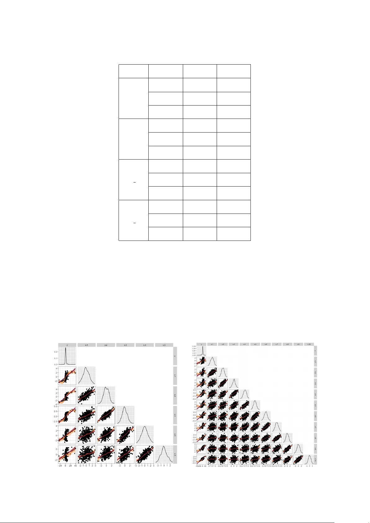
High-dimensional sparse vine copula regression with application to genomic prediction ¨ Ozge Sahin ∗ Departmen t of Mathematics, T ec hnical Univ ersit y of Munic h, Boltzmanstraße 3, Garc hing, German y Claudia Czado Departmen t of Mathematics, T ec hnical Univ ersit y of Munic h, Boltzmanstraße 3, Garc hing, German y Munic h Data Science Institute, W alther-v on-Dyc k-Straße 10, Garc hing, German y Abstract High-dimensional data sets are often a v ailable in genome-enabled predictions. Suc h data sets include nonlinear relationships with complex dependence structures. F or suc h situations, vine copula based (quan tile) regression is an imp ortan t to ol. Ho w ev er, the curren t vine copula based regression approaches do not scale up to high and ultra-high dimensions. T o p erform high-dimensional sparse vine copula based regression, w e prop ose t w o metho ds. First, w e sho w their sup eriorit y re- garding computational complexity ov er the existing metho ds. Second, we deﬁne relev ant, irrelev an t, and redundant explanatory v ariables for quantile regression. Then we show our method’s p o wer in selecting relev ant v ariables and prediction accuracy in high-dimensional sparse data sets via simulation studies. Next, we ap- ply the prop osed methods to the high-dimensional real data, aiming at the genomic prediction of maize traits. Some data-pro cessing and feature extraction steps for the real data are further discussed. Finally , we show the adv antage of our metho ds o v er linear mo dels and quantile regression forests in sim ulation studies and real data applications. Keywor ds : Genomic prediction; High-dimensional data; V ariable selection; Vine copula; Quan tile regression ∗ Corresp onding author: ozgesahin-94@hotmail.com 1 1 In tro duction Genomic prediction (GP) aims at predicting a breeding v alue using genotypic measure- men ts. Then an unobserv ed trait is predicted using its genotype information lik e single- n ucleotide p olymorphism (SNP). With rapid dev elopments in genomic technologies, re- searc hers ha v e high-dimensional SNP data sets. Ho w ever, it p oses some c hallenges in prediction mo deling, such as a small num b er of observ ations and a large n um b er of ex- planatory v ariables, sk ewness in v ariables, irrelev ant and redundan t v ariables, in teractions among v ariables, and nonconstant error v ariance. T o s olv e the drawbac ks regarding the data dimensionalit y in the GP , statistical or mac hine learning based approaches hav e b een applied (Li et al. 2018 ). Recently , quan tile regression approaches, whic h mo del the conditional distribution of the response, ha ve b een utilized to deal with the sk ewness and outliers in the data (P´ erez-Ro dr ´ ıguez et al. 2020 ). Still, the question has b een how to mo del c onditional quantiles ﬂexibly while hand ling data dimensionality in GP . It is also imp ortan t to identify the SNPs r elevant for predicting breeding v alues to design future genotype studies. F or instance, since the human p opulation has b een grow- ing, the stabilit y of fo od supplies has gained muc h more imp ortance. Hence, recen t plant breeding eﬀorts aim at the genetic impro v emen t of crops. H¨ olk er et al. ( 2019 ) provided agronomic measuremen ts and more than 500 thousand SNPs to mak e Europ ean ﬂin t maize landraces a v ailable for such an aim. Vine copula based (quantile) regression allo ws mo deling a nonlinear relationship b e- t w een explanatory v ariables and resp onse. It considers higher-order explanatory v ariables and deals with unknown functional error forms. Ho wev er, the current vine copula based regression metho ds’ computational complexit y makes them infeasible to b e applied in high-dimensional data sets (Kraus and Czado 2017 ; T ep eg jozo v a et al. 2022 ). W e refer to high- and ultra high- dimensional data sets when the num b er of explanatory v ariables is b et w een ten and 1000 and larger than 1000, resp ectiv ely . W e prop ose t wo vine copula based regression metho ds that perform well in analyzing high-dimensional sparse data sets, where sparsit y means that man y explanatory v ariables do not predict the resp onse. Their computational complexit y is signiﬁcan tly less than the existing metho ds. W e deﬁne relev an t, redundan t, and irrelev ant explanatory v ariables for quan tile regression and assess the metho ds’ prediction p o w er in high-dimensional sparse sim ulated data sets. Our analyses regarding the inclusion of relev ant v ariables and exclu- 2 sion of irrelev ant v ariables show our metho ds’ capabilit y to provide sparse mo dels. W e apply the metho ds for genomic prediction of maize traits, prop osing data prepro cessing and feature extraction steps on the data given by H¨ olk er et al. ( 2019 ). Suc h steps can b e further applied and improv ed in future studies. Overall, we can resolv e data dimension- alit y issues in vine copula based regression. T o the b est of our kno wledge, there has not y et b een any study p erforming the genomic prediction using vine copula mo dels, as w ell as assessing vine copula regression metho ds’ p erformance in the presence of redundan t and irrelev ant v ariables. Alternativ e nonlinear quan tile regression models are generalized additiv e mo dels ( GAM ) (W o o d 2017 ), quantile regression forests ( QRF ) (Meinshausen 2006 ), and quantile regres- sion neural net works ( QRN N ) (Cannon 2011 ). QR N N may suﬀer from quan tile crossing (Cannon 2018 ), whic h do es not exist in vine copula based approaches b y construction. Kraus and Czado ( 2017 ) sho w a b etter p erformance of their vine copula based approach than GAM . Hence, among nonlinear mo dels, we compare our models with quantile regression forests and sho w our adv an tages, esp ecially in the presence of dep enden t v ari- ables. Moreov er, despite the quan tile crossing problem, w e analyze the p erformance of linear mo dels with v ariable selection, i.e., linear quantile regression with a LASSO type p enalt y ( LQRLasso ) (Sherwoo d and Maidman 2020 ), in nonlinear cases. The pap er is organized as follo ws: Section 2 in tro duces vine copulas and new metho ds; Section 3 provides sim ulation studies. W e present the real data application in Section 4 , discuss our ﬁndings and conclude in Section 5 . 2 High-dimensional sparse vine copula regression 2.1 D-vine copulas and prediction Copulas are distribution functions, allo wing us to separate the univ ariate margins and dep endence structure. Let X = ( X 1 , . . . , X p ) ⊤ ∈ R p b e a p -dimensional random vector with the joint cumulativ e distribution function (cdf ) F and the univ ariate marginal distri- butions F 1 , . . . F p . By Sklar’s theorem (Sklar 1959 ), the copula C , corresp onding to F , is a multiv ariate cdf with uniform margins such that F ( x 1 , . . . , x p ) = C  F 1 ( x 1 ) , . . . F p ( x p )  . When the univ ariate marginal distributions are con tin uous, C is unique, whic h w e as- sume in the remainder. In addition, the p -dimensional join t density f can b e written as 3 f ( x ) = c  F 1 ( x 1 ) , . . . , F p ( x p )  · f 1 ( x 1 ) · · · f p ( x p ) , x ∈ R p , where c is the copula density of the random v ector  F 1 ( X 1 ) , . . . F p ( X p )  ⊤ ∈ [0 , 1] p . Standard m ultiv ariate copulas, such as the multiv ariate exc hangeable Arc himedean or Gaussian, often do not accurately mo del the dependence among the v ariables. Aas et al. ( 2009 ) developed a pair-copula construction or vine copula approac h using a cascade of biv ariate copulas to extend their ﬂexibilities. Suc h a construction can b e represented by an undirected graphical structure in volving a set of linked trees, i.e., a regular (R-) vine (Bedford and Co ok e 2002 ). A R-vine for p v ariables consists of p − 1 trees, where the edges in the ﬁrst tree are the no des of the second tree, the edges of the second tree are the no des of the third tree and so on. If an edge connects tw o no des in the ( t + 1)th tree, their asso ciated edges in the t th tree m ust hav e a shared node in the t th tree for t = 1 , . . . , p − 2. The no des and edges in the ﬁrst tree represen t p v ariables and unconditional dep endence for p − 1 pairs of v ariables, resp ectiv ely . In the higher trees, the conditional dep endence of a pair of v ariables conditioning on other v ariables is mo deled. T o get a vine copula or pair-copula construction, there is a biv ariate (pair) copula asso ciated with eac h edge in the vine. One sp ecial class of R-vines are D-vines, whose graph structure is a path, i.e., all no des’ degree in the graph is smaller than three. A no de in a path represen ts a v ariable, and an edge b etw een a pair of no des corresp onds to dep endence among the v ariables of the respective no des expressed by a pair copula. The no de having a degree of one is called a leaf no de. Once the order of the no des in the ﬁrst tree is determined, the asso ciated D-vine copula decomp osition is unique. Moreo ver, if the pair copulas in the higher tree lev els than t are indep endence copulas, where t < p and t ≥ 1, represen ting conditional indep endence, a t -truncated vine copula is obtained as sho wn App endix in A . D-vine copulas allo w to express the conditional densit y of a leaf node in the ﬁrst tree in a closed form. Here we choose the leaf no de in the ﬁrst tree of a D-vine copula as a resp onse v ariable. In the remainder, assume that ( y i , x i, 1 , . . . , x i,p ), i = 1 , . . . , n , are realizations of the random vector ( Y , X 1 , . . . , X p ), and Y denotes a resp onse v ari- able with its marginal distributions F Y and the others corresp ond to explanatory v ari- ables with their marginal distributions F 1 , . . . , F p . F or the D-vine copula with the no de order 0 − 1 − . . . − p corresp onding to the v ariables Y − X 1 − . . . − X p , p ≥ 2, as stated in Kraus and Czado ( 2017 ), the conditional quantile function F − 1 0 | 1 ,...,p at quantile 4 α can b e expressed in terms of the in v erse marginal distribution function F − 1 Y of the resp onse and the conditional D-vine copula quan tile function C − 1 0 | 1 ,...,p at quantile α as F − 1 0 | 1 ,...,p ( α | x 1 , . . . , x p ) = F − 1 Y  C − 1 0 | 1 ,...,p ( α | F 1 ( x 1 ) , . . . , F p ( x p )  . Since p -dimensional D-vine copula’s input is the marginally uniform data on [0 , 1] p , the estimation of the D-vine copula follo ws a t w o-step approach called the inference for mar- gins (Jo e and Xu 1996 ). First, each marginal distribution is estimated. Then the data is con v erted in to the copula data b y applying probabilit y in tegral transformation, e.g., using a univ ariate non-parametric kernel densit y estimator, i.e., ˆ F Y and ˆ F X d , d = 1 , . . . , p . Next, w e hav e the pseudo copula data: ( v i , u i, 1 , . . . , u i,p ) = ( ˆ F Y ( y i ) , ˆ F X 1 ( x i, 1 ) , . . . , ˆ F X p ( x i,p )), i = 1 , . . . , n , b eing realizations of the random vector ( V , U 1 , . . . , U p ). More details ab out the conditional log-likelihoo d and estimation of D-vine copulas are given in App endix A . 2.2 Prop osed metho ds: v iner eg Res and v iner eg P ar C or W e propose t wo methods to p erform a D-vine copula regression on high-dimensional sparse data sets: v iner eg Res and v iner eg P ar C or . Appendices B and C giv e an illustra- tiv e example and details of the metho ds. The metho d v iner eg Res p erforms the v ariable selection at a given iteration based on the residuals of the previous iteration, i.e., the pseudo-resp onse. It ﬁnds the v ariable among the candidates, whic h provides the best biv ariate copula conditional log-lik eliho o d conditioned on the v ariable and conditioning the pseudo-resp onse of the previous itera- tion. Assume ˜ y ( s ) i and ˜ v ( s ) i i = 1 , . . . , n , denote the pseudo-resp onse and its pseudo copula data in the s th iteration, resp ectiv ely , which are realizations of the random v ariable Y ( s ) and V ( s ) , resp ectiv ely . V (0) and V ( s ) ha v e the indices 0 and 0 ( s ) , resp ectiv ely , and are alw a ys a leaf no de in the ﬁrst tree. v iner eg Res S tep 1 (initialization): F or giv en data ( y i , x i, 1 , . . . , x i,p ) and ( v i , u i, 1 , . . . , u i,p ), deﬁne the initial pseudo-resp onse ˜ y (1) i = y i with its copula scale ˜ v (1) i , i = 1 , . . . , n , the initial D-vine order D (1) = (0), the initial c hosen v ariable index set I (1) v ar = ∅ , and the initial set of candidate explanatory v ariables p (1) cand = { 1 , . . . , p } . F or s = 1 , 2 , . . . , S tep 2 (v ariable selection): Fit a parametric biv ariate copula to data { ( ˜ v ( s ) i , u i,d ), i = 1 , . . . , n } for d ∈ p ( s ) cand and denote the copula, copula densit y , and its estimated 5 parameters b y d C R d ( s ) , b cr d ( s ) and ˆ θ d ( s ) , resp ectiv ely . Then, ﬁnd the v ariable for whic h the conditional log-likelihoo d of the copula d C R d ∗ ( s ) is maximized, i.e., d ∗ ( s +1) = arg max d ( s ) ∈ p ( s ) cand P n i =1 ln b cr d ( s ) 0 ( s ) | d ( s ) ( ˜ v ( s ) i | u i,d ( s ) ; ˆ θ d ( s ) ) . S tep 3 (D-vine extension): Extend the D-vine order b y adding the v ariable with index d ∗ ( s +1) to get a D-vine order D ( s +1) = ( D ( s ) , d ∗ ( s +1) ). Select the parametric pair copula families and estimate the parameters in the extended D-vine structure, where the asso ciated D-vine copula and its estimated parameters are denoted by ˆ C ( s +1) and ˆ θ ( s +1) , resp ectiv ely . S tep 4 (Chosen v ariable indices and h yp erparameter up dates): Extend the c hosen v ariable set, adding the new v ariable, I ( s +1) v ar = I ( s ) v ar ∪ d ∗ ( s +1) and up date p ( s +1) cand = p ( s ) cand \ d ∗ ( s +1) . S tep 5 (Pseudo-resp onse up date or stop): If a stopping condition (Section 2.4 ) do es not hold, estimate the median of the resp onse v ariable based on the D-vine copula ˆ C ( s +1) and up date the pseudo-resp onse, i.e., ˜ y ( s +1) i = y i − ˆ F − 1 Y ( ˆ C − 1( s +1) 0 | I ( s +1) var (0 . 50 | u i,p 1 , . . . , u i,p d ( s +1) ; ˆ θ ( s +1) )) , ˜ v ( s +1) i = ˆ F Y ( s +1) ( ˜ y ( s +1) i ) , where i = 1 , . . . , n and { p 1 , . . . , p d ( s +1) } ⊆ I ( s +1) v ar . Another metho d to p erform an eﬃcien t D-vine copula regression for high-dimensional data is to use the partial correlation b et w een the resp onse and a candidate explanatory v ariable giv en the chosen v ariables at eac h iteration based on their empirical normal scores. Suc h scores are calculated as detailed in Section 1 of Jo e ( 2014 ). v iner eg P ar C or S tep 1 (initialization): As giv en in v iner eg Res and the data’s normal scores. F or s = 1 , 2 , . . . , S tep 2 (v ariable selection): d ∗ ( s +1) = arg max d ( s ) ∈ p ( s ) cand | ˆ ρ 0 ,d ( s ) ; I ( s ) var | , where ˆ ρ j,k ; S is the estimated partial correlation of v ariables j, k giv en those indexed in S based normal scores. S tep 3 (D-vine extension): As giv en in v iner eg Res . S tep 4 (Chosen v ariable indices and h yp erparameter up dates): As giv en in v inereg Res . 2.3 Biv ariate copula selection Step 3 of v iner eg Res and v iner eg P ar C or selects parametric pair copulas and estimates their parameters asso ciated with the extension of the D-vine structure. Also, Step 2 of 6 v iner eg Res ﬁts a parametric biv ariate copula to the pseudo-resp onse and a candidate explanatory v ariable. First, w e estimate the parameters that maximize the log-likelihoo d of a candidate biv ariate copula family , whic h is listed in App endix D . Later w e can select the one with the lo west Ak aik e (AIC) or the Bay esian information criterion. While extending the D-vine structure and adding new trees at Step 3 of the metho ds, the ﬁt of parametric pair copulas can b e p erformed sequentially from the low est to the highest trees (Brechmann 2010 ). 2.4 Stopping criteria T o decide if a chosen candidate explanatory v ariable in a given iteration should b e in a mo del, we will consider the conditional AIC, whic h p enalizes the conditional log-lik eliho o d of the mo del based on the D-vine copula b y the eﬀectiv e degrees of freedom in the mo del whose details are pro vided in App endix D . W e stop adding v ariables in D-vine copula regressions when the current iteration’s conditional AIC is equal to or larger than the previous iteration’s conditional AIC. If the conditional AIC alw ays improv es in each iteration, we stop after all explanatory v ariables are included in the model. 2.5 Complexit y Assuming that the data consists of p explanatory v ariables, the complexity of the ex- isting metho d v iner eg is O ( p 3 ) in terms of the total num b er of biv ariate copulas to b e selected during the algorithm (T ep eg jozo v a 2019 ). Thus, we ev aluate the complexity of v iner eg Res and v iner eg P ar C or using the same criterion. W e will consider the w orst case scenario that the algorithms run un til all explanatory v ariables are included in the mo del. F urther, the total num b er of estimated parameters is linear in terms of the num b er of biv ariate copulas. The detailed calculations in Appendix D show that the complexit y of v iner eg P ar C or and viner eg Res in terms of the total n um b er of selected biv ariate copulas is O ( p 2 ). Hence, our metho ds signiﬁcantly reduce the computational complexity of v iner eg . 7 2.6 Relev an t, redundan t, and irrelev an t v ariables No w w e deﬁne relev ant, redundan t, and irrelev ant v ariables for predicting the conditional quan tile of a resp onse v ariable Y given the index set of explanatory v ariables X . W e will denote the cdf of the v ariables with the index set X b y F X in the follo wing. Deﬁnition 2.1 (R elevant variables) The index set of variables M ⊆ X is c al le d r elevant for Y if and only if it holds F Y |M ( y | x M )  = F Y ( y ) , wher e x M includes the variables in M . Deﬁnition 2.2 (R e dundant variables) The index set of variables R is c al le d r e dun- dant given the set of variables M for Y if and only if it holds F Y |M , R ( y | x M , x R ) = F Y |M ( y | x M ) and F M , R ( x M , x R )  = F M ( x M ) · F R ( x R ) , wher e the ve ctors x M and x R include the variables in the sets M and R , r esp e ctively, R ⊆ X , M ⊆ X , R ∩ M = ∅ . A discussion on redundant v ariables in a D-vine copula is in Appendix E . Example 2.1 Consider the mo del ( Y , X 1 , X 2 ) ⊤ ∼ N 3 ( 0 , Σ) with (0.5, 0.4, 0.8) ve ctor- izing the upp er triangular p art of the symmetric c ovarianc e matrix Σ , wher e it holds ρ Y ,X 2 ; X 1 = 0 , i.e., Y is c onditional ly indep endent of X 2 given X 1 . Henc e, we have f Y | X 1 ,X 2 ( y | x 1 , x 2 ) = f Y ,X 2 | X 1 ( y ,x 2 | x 1 ) f X 2 | X 1 ( x 2 | x 1 ) = f Y | X 1 ( y | x 1 ) · f X 2 | X 1 ( x 2 | x 1 ) f X 2 | X 1 ( x 2 | x 1 ) = f Y | X 1 ( y | x 1 ) . Sinc e f X 1 ,X 2 ( x 1 , x 2 )  = f X 1 ( x 1 ) · f X 2 ( x 2 ) , X 2 is r e dundant given X 1 for Y . Deﬁnition 2.3 (Irr elevant variables) The set of variables I is c al le d irr elevant given the set of variables M for Y if and only if it holds F Y |M , I ( y | x M , x I ) = F Y |M ( y | x M ) , F M , I ( x M , x I ) = F M ( x M ) · F I ( x I ) , and F Y , I ( y , x I ) = F Y ( y ) · F I ( x I ) , wher e the ve ctors x M and x I include the variables in the sets M and I , r esp e ctively, I ⊆ X , M ⊆ X , I ∩ M = ∅ . Example 2.2 Consider the mo del ( Y , X 1 , X 2 ) ⊤ ∼ N 3 ( 0 , Σ) with (0.5, 0, 0) ve ctorizing the upp er triangular p art of the symmetric c ovarianc e matrix Σ , wher e it holds ρ Y ,X 2 ; X 1 = 0 ; henc e, f Y | X 1 ,X 2 ( y | x 1 , x 2 ) = f Y | X 1 ( y | x 1 ) . In addition, it holds f X 1 ,X 2 ( x 1 , x 2 ) = f X 1 ( x 1 ) · f X 2 ( x 2 ) and f Y ,X 2 ( y , x 2 ) = f Y ( y ) · f X 2 ( x 2 ) ; thus, X 2 is irr elevant given X 1 for Y . 8 3 Sim ulation study W e sho w the ﬂexibilit y and eﬀectiveness of the prop osed metho ds on simulated datasets b eing nonlinear and ha ving diﬀerent sparsit y . W e explore the follo wing questions: (Q1) Ho w do v iner eg Res and v iner eg P ar C or work in situations with nonlinear explanatory v ariable eﬀects on the resp onse’s quan tiles in the presence of redundan t and irrelev ant v ariables for prediction accuracy and computational complexit y? (Q2) Ho w w ell do v iner eg Res and v iner eg P ar C or identify relev ant and irrelev ant v ariables for predict- ing the response’s quantiles? (Q3) Ho w do v iner eg Res and v iner eg P ar C or perform compared to the alternativ e metho ds LQRLasso and QRF introduced and discussed in App endix F ? 3.1 Data generating pro cess (DGP) DGP1: irrelev an t v ariables Y d i = X i, 1 · X 2 i, 2 · q | X i, 3 | + 0 . 1 + e 0 . 4 · X i, 4 · X i, 5 + ( X i, 6 , . . . , X i,p d )(0 , . . . , 0) ⊤ + ϵ i · σ i , i = 1 , . . . , n, d = 1 , 2 , 3 , (1) where we sample the relev ant v ariables ( X i, 1 , . . . , X i, 5 ) ⊤ ∼ N 5 ( 0 , Σ), i = 1 , . . . , n with the ( a, b )th elemen t of the cov ariance matrix Σ a,b = 0 . 75 | a − b | , irrelev ant v ariables ( X i, 6 , . . . , X i,p d ) ⊤ ∼ N p d − 5 ( 0 , I p d − 5 ), the random error terms ϵ i ∼ N (0 , 1) that are in- dep enden t and iden tically distributed (iid), indep enden tly , and set σ i ∈ { 0 . 5 , 1 } , i = 1 , . . . , n . W e sim ulate data sets with diﬀeren t num b er of irrelev ant v ariables and set it to ( p d − 5) in each case d = 1 , 2 , 3 as follows: Case 1 with p 1 = 10 (50% of v ariables are irrelev ant), Case 2 with p 2 = 20 (75% of v ariables are irrelev ant), Case 3 with p 3 = 50 (90% of v ariables are irrelev ant). DGP2: redundan t v ariables Y d i = q | 5 · X i, 1 − 2 · X i, 9 + 0 . 5 | + X i, 8 · ( − 4 · X i, 3 + 1) + e X i, 6 + (2 · X 3 i, 10 + X 3 i, 4 ) + ( X i, 7 + 1) · (ln ( | X i, 2 + X i, 5 | + 0 . 01))+ ( X i, 11 , . . . , X i,p d )(0 , . . . , 0) ⊤ + ϵ i · σ i , i = 1 , . . . , n, d = 1 , 2 , 3 , 4 , (2) where the samples of explanatory v ariables are indep enden tly generated from a multi- v ariate normal distribution with a T o eplitz correlation structure, i.e., ( X i, 1 , . . . , X i,p d ) ⊤ ∼ 9 N p d ( 0 , Σ), i = 1 , . . . , n , j = 1 , 2 , 3, with the ( a, b )th element of the co v ariance matrix Σ a,b = ρ | a − b | . T o represen t a c hallenging but realistic scenario, w e set ρ = 0 . 75. W e sample ϵ i ∼ N (0 , 1), i = 1 , . . . , n (iid) indep enden tly from the explanatory v ariables and set σ i ∈ { 0 . 5 , 1 } , i = 1 , . . . , n . All v ariables are predicting the resp onse’s quantiles; ho w ever, giv en the ﬁrst ten v ariables, the others are redundant. W e change the num b er of redundant v ariables and set it to ( p d − 10) for d = 1 , 2 , 3 , 4: Case 1 with p 1 = 20 (50% of v ariables are redundan t given the ten relev ant ones), Case 2 with p 2 = 40 (75% of v ariables are redundan t giv en the ten relev an t ones), Case 3 with p 3 = 100 (90% of v ariables are redundant giv en the ten relev ant ones), Case 4 with p 4 = 1000 (99% of v ariables are redundant given the ten relev ant ones). Based on the DGPs in Equations ( 1 ) and ( 2 ), w e simulate samples with size 450 ( n =450) with a random split of 300/150 observ ations for a training/a test set. W e replicate our pro cedure 100 times and av erage p erformance measures p er sample, which are deﬁned in App endix F . 3.2 P erformance measures W e consider the computation time, the n um b er of c hosen v ariables, true p ositive r ate (TPR ), and false disc overy r ate (FDR) as metho ds’ p erformance measures on the training set. T o ev aluate the p erformance of a metho d on the test set, w e apply the pinb al l loss ( P L α ) at α = 0 . 05 , 0 . 50 , 0 . 95. TPR is the ratio of the num b er of chosen relev ant v ariables by a metho d M to the total num b er of relev an t v ariables. FDR is the ratio of the num b er of c hosen irrelev an t v ariables to the total num b er of c hosen v ariables by a metho d M . Higher TPR and smaller FDR are b etter. P L α measures the accuracy of the quantile predictions ˆ y α,M i at the level α by a metho d M compared to the giv en resp onse y i , i = 1 , . . . , n . The pinball loss is identical to chec k score, and smaller pinball loss v alues are b etter (Steinw art and Christmann 2011 ). The formal deﬁnitions are giv en in App endix F . 3.3 Results All computations are run on a single no de CPU with Intel Xeon Platin um 8380H Pro cessor with around 25 GB RAM, running R v ersion 4.2.2. Ho wev er, Step 2 of v iner eg Res can b e brok en down in to parallel ﬁts across candidate v ariables for a faster computation. 10 V ariable sele ction and c omputational c omplexity r esults on the tr aining set : In T able 1 , we analyze the TPR and FDR only for the DGP1 setting since all v ariables are rele- v ant in the DGP2 setting. The computations for v iner eg did not complete within three da ys p er replication for the fourth case of the DGP2 setting, making it computationally infeasible. Also, we did not run LQR Lasso for that case since it ran around seven hours p er replication and had w orse p erformances in the other sim ulation cases. In all cases, QRF chooses all v ariables in the asso ciated DGP to make predictions. Th us, its TPR is one, the num b er of selected v ariables equals the total num b er of v ariables in a sample, and its FDR is the prop ortion of the irrelev an t v ariables in the asso ciated DGP setting. More analyses ab out QRF are pro vided in App endix G . Excluding QRF , in all cases of the DGP1 setting, v iner eg has a b etter TPR p erfor- mance than the others. Ho w ever, its FDR is higher than others, adding many irrelev ant v ariables to the mo del. v inereg Res correctly identiﬁes more than 75% of the relev an t v ariables in all cases of the DGP1 setting. Its FDR is less than 15% there, making it the b est metho d for FDR. F urther, v iner eg P ar C or ’s TPR is higher than 50% in all DGP1 cases. How ever, lik e others, its FDR increases as the num b er of irrelev ant v ariables increases in the mo del, reac hing more than 50% in the third DGP1 case. LQRLasso iden tiﬁes at least 48% of the relev an t v ariables, but its TPR decreases when the num b er of irrelev ant v ariables increases. While v iner eg Res selects the lo w est n um b er of v ariables b et ween four and six, viner eg includes almost half of the total n umber of v ariables in the data in eac h case. This highligh ts the p o wer of v iner eg Res regarding the exclusion of irrelev ant v ariables in sparse data sets. v iner eg P ar C or ’s num b er of chosen v ariables is b et ween v iner eg and v iner eg Res in all ev aluated cases. The same applies to LQRLasso , but it selects more v ariables for estimating median predictions than other quan tiles. In an ultra high- dimensional case with 1000 explanatory v ariables, the n um b er of v ariables chosen b y v iner eg P ar C or is, on a verage, 31.72 with the empirical standard error of 1.23 while it is 7.08 with that of 0.54 for v iner eg Res . As the n um b er of v ariables increases, the a v erage running time for all metho ds in- creases. Among vine based metho ds, v iner eg P ar C or pro vides the fastest computation as exp ected from the results in Section 2.5 . Ho wev er, QR F pro vides the fastest compu- tation among all metho ds considered. v iner eg Res and v iner eg P ar C or run less than 15 11 min utes in the ultra high-dimensional case. LQRLasso ’s running time for quan tile lev els do es not diﬀer muc h. T able 1: Comparison of the metho ds’ p erformance on the training set ov er 100 replications under the cases 1—3 and 1—4 sp eciﬁed in Equations ( 1 ) and ( 2 ), resp ectiv ely . The n um b ers in parentheses under a metho d’s name column are the corresp onding empirical standard errors. (-) sho ws computational infeasibility . LQR Lasso column corresp onds to the quan tile levels (0.05, 0.50, 0.95). Chosen V ars. corresp onds to the total num b er of c hosen v ariables. Time is in min utes and p er replication. DGP Measure Case v inereg v inereg Res v inereg P ar C or QRF LQRLasso (0.05, 0.50, 0.95) 1 TPR 1 0.81 (0.01) 0.80 (0.02) 0.67 (0.02) 1.00 (0.00) 0.73 (0.02), 0.69 (0.02), 0.63 (0.02) 2 0.85 (0.01) 0.79 (0.03) 0.59 (0.02) 1.00 (0.00) 0.68 (0.02), 0.68 (0.02), 0.55 (0.02) 3 0.89 (0.01) 0.78 (0.02) 0.56 (0.02) 1.00 (0.00) 0.61 (0.02), 0.61 (0.02), 0.48 (0.01) FDR 1 0.28 (0.01) 0.08 (0.01) 0.24 (0.02) 0.50 (0.00) 0.28 (0.02), 0.32 (0.02), 0.24 (0.02) 2 0.55 (0.01) 0.13 (0.02) 0.45 (0.02) 0.75 (0.00) 0.38 (0.02), 0.49 (0.03), 0.34 (0.03) 3 0.80 (0.00) 0.15 (0.02) 0.65 (0.02) 0.90 (0.00) 0.35 (0.03), 0.58 (0.02), 0.40 (0.03) Chosen V ars. 1 5.83 (0.13) 4.56 (0.19) 4.68 (0.16) 10.00 (0.00) 5.24 (0.22), 5.48 (0.21), 4.99 (0.26) 2 9.76 (0.19) 5.04 (0.26) 6.03 (0.23) 20.00 (0.00) 6.60 (0.41), 8.48 (0.43), 5.30 (0.36) 3 23.24 (0.42) 5.29 (0.33) 8.74 (0.30) 50.00 (0.00) 5.93 (0.38), 10.20 (0.68), 5.97 (0.47) Time 1 0.18 (0.00) 0.17 (0.01) 0.06 (0.00) 0.01 (0.00) 0.02 (0.00), 0.02 (0.00), 0.02 (0.00) 2 0.97 (0.02) 0.30 (0.02) 0.10 (0.01) 0.01 (0.00) 0.02 (0.00), 0.43 (0.03), 0.02 (0.00) 3 12.06 (0.31) 0.77 (0.05) 0.34 (0.03) 0.03 (0.00) 0.12 (0.00), 0.14 (0.00), 0.12 (0.00) 2 Chosen V ars. 1 10.94 (0.23) 5.41 (0.19) 6.68 (0.20) 20.00 (0.00) 7.05 (0.32), 10.12 (0.36), 8.95 (0.40) 2 19.63 (0.54) 5.17 (0.17) 8.25 (0.28) 40.00 (0.00) 7.88 (0.43), 12.36 (0.51), 9.88 (0.48) 3 62.92 (2.78) 5.83 (0.22) 11.66 (0.42) 100.00 (0.00) 7.35 (0.36), 15.45 (0.78), 9.44 (0.55) 4 - 7.08 (0.54) 31.72 (1.23) 1000.00 (0.00) - Time 1 1.15 (0.03) 0.20 (0.01) 0.16 (0.01) 0.01 (0.00) 0.09 (0.00), 0.10 (0.00), 0.08 (0.00) 2 7.30 (0.26) 0.32 (0.01) 0.29 (0.03) 0.02 (0.00) 0.11 (0.00), 0.13 (0.00), 0.11 (0.00) 3 159.22 (8.66) 0.84 (0.03) 0.72 (0.06) 0.05 (0.00) 0.35 (0.00), 0.35 (0.00), 0.34 (0.00) 4 - 9.44 (0.69) 12.18 (1.26) 0.44 (0.00) - Pr e diction ac cur acy r esults on the test set : T able 2 sho ws that v iner eg Res provides the b est ﬁt in eigh t ev aluations out of nine (three pinball losses ev aluated for three levels) in the DGP1 setting among vine copula based metho ds. v iner eg and v iner eg P ar C or ha v e the same accuracy as v iner eg Res for the ﬁrst case in the DGP1 setting. Ho wev er, as the num b er of irrelev ant v ariables increases, a residual-based v ariable selection ma y b e b etter than other vine copula based metho ds. Moreo v er, LQRLasso has the highest pin ball loss in all cases of the DGP1 setting b ecause of the high nonlinearit y in samples. Ev en though v inereg P ar C or ’s p erformance is b etter than LQRLasso , it pro vides w orse ﬁts than the others at the lev el 95%. A lik ely explanation can be that including irrelev an t 12 v ariables in addition to the most relev ant ones in a vine copula may negatively impact the prediction accuracy . How ev er, a similar result does not apply to QRF . Despite including all irrelev an t v ariables in the mo del, QRF still p erforms b etter than all in sev en ev aluations out of nine. T able 2 sho ws that v iner eg Res provides the lo west pin ball loss at three quan tile levels in all DGP2 cases, except at the lev el 95% in the ﬁrst case. Since v iner eg Res giv es the most sparse mo dels in the DGP2 setting in T able 1 , w e infer t hat including man y relev ant but p oten tially redundant v ariables in v inereg , v iner eg P ar C or , and QR F is worsening the prediction accuracy in the DGP2 setting. LQRLasso suﬀers from nonlinearity . Since the relev ant, irrelev an t, and redundant v ariables are kno wn in simulation studies, when only the relev ant ten v ariables are used for prediction in the DGP2 setting, QR F has the pinball loss of 0.64, 1.81, and 0.62 at lev els 0 . 05 , 0 . 50 , and 0 . 95, resp ectiv ely . Th us, viner eg Res w ould hav e b etter accuracy than QRF in most cases of the DGP2 setting, ev en if the latter selected the most relev an t v ariables. Th us, v iner eg Res is more adv antageous than QR F in the presence of many dep enden t v ariables in our sim ulations. 13 T able 2: Comparison of the av erage p erformance of the metho ds on the test set for the pin ball loss ( P L α ) at diﬀeren t quan tile levels α o ver 100 replications under the cases 1—3 and 1—4 sp eciﬁed in Equations ( 1 ) and ( 2 ), resp ectiv ely . The b est p erformance for eac h quan tile level and DGP case is highlighted. The num b ers in parentheses under a metho d’s name column are the corresp onding empirical standard errors. (-) sho ws computational infeasibilit y . DGP Measure Case v inereg v iner egR es v inereg P ar C or QRF LQRLasso 1 P L 0 . 05 1 0.21 (0.01) 0.21 (0.01) 0.21 (0.01) 0.22 (0.01) 0.34 (0.01) 2 0.23 (0.01) 0.22 (0.01) 0.22 (0.01) 0.22 (0.01) 0.34 (0.02) 3 0.24 (0.01) 0.21 (0.01) 0.22 (0.01) 0.22 (0.01) 0.32 (0.01) P L 0 . 50 1 0.79 (0.04) 0.79 (0.03) 0.81 (0.04) 0.76 (0.04) 0.94 (0.02) 2 0.84 (0.04) 0.79 (0.03) 0.82 (0.04) 0.69 (0.02) 0.97 (0.04) 3 0.84 (0.02) 0.76 (0.02) 0.79 (0.02) 0.72 (0.02) 0.90 (0.02) P L 0 . 95 1 0.43 (0.07) 0.43 (0.06) 0.46 (0.07) 0.41 (0.07) 0.59 (0.04) 2 0.37 (0.04) 0.39 (0.04) 0.44 (0.04) 0.32 (0.03) 0.64 (0.07) 3 0.38 (0.03) 0.38 (0.03) 0.41 (0.03) 0.35 (0.03) 0.53 (0.03) 2 P L 0 . 05 1 0.53 (0.01) 0.53 (0.01) 0.54 (0.01) 0.70 (0.02) 0.84 (0.02) 2 0.57 (0.01) 0.54 (0.01) 0.56 (0.01) 0.70 (0.02) 0.85 (0.02) 3 0.81 (0.04) 0.54 (0.01) 0.58 (0.01) 0.72 (0.01) 0.92 (0.03) 4 - 0.55 (0.01) 0.89 (0.02) 0.78 (0.02) - P L 0 . 50 1 1.87 (0.02) 1.83 (0.02) 1.84 (0.02) 1.91 (0.02) 2.20 (0.02) 2 1.99 (0.02) 1.84 (0.02) 1.86 (0.02) 1.93 (0.03) 2.26 (0.03) 3 2.59 (0.09) 1.84 (0.02) 1.94 (0.02) 2.00 (0.03) 2.29 (0.02) 4 - 1.89 (0.03) 2.42 (0.03) 2.17 (0.03) - P L 0 . 95 1 0.53 (0.01) 0.55 (0.01) 0.55 (0.01) 0.65 (0.01) 0.78 (0.02) 2 0.57 (0.01) 0.56 (0.01) 0.56 (0.01) 0.67 (0.01) 0.82 (0.02) 3 0.81 (0.05) 0.57 (0.01) 0.61 (0.02) 0.68 (0.01) 0.83 (0.02) 4 - 0.57 (0.02) 0.88 (0.03) 0.75 (0.02) - 4 Application: the genomic prediction of maize traits W e describ e a real-data application on the doubled-haploid (DH) lines from Europ ean ﬂin t maize landraces that motiv ates our metho ds’ usage. H¨ olk er et al. ( 2019 ) ev aluated 14 899 DH lines whose data contains genot ypic measurements with the SNP array technology and phenotypic measuremen ts of agronomic traits across environmen ts. W e are in terested in the relationship b et w een a DH line’s genotype enco ded by its SNPs and its phenot ypic outcome describ ed b y its traits, i.e., the genomic prediction of maize traits. Sp eciﬁcally , we w ould like to ﬁnd relev ant SNPs for a trait in a multiv ariate prediction mo del using our high-dimensional vine copula regression metho ds, p erforming v ariable selection. 4.1 Data description and prepro cessing There are three landraces in the data, and we focus on the Kemater Landmais Gelb (KE) landrace, whic h has the largest num b er of observ ations (471 out of 899). There are 501,124 explanatory v ariables, SNPs, which ha ve only zero and tw o as v alues, e.g., zero corresp onds to the genot yp e TT, and tw o denotes the genot yp e CC. W e predict four resp onses of agronomic traits separately: early plan t heigh t measured b y cen timetres at the fourth and sixth stages (PH V4/V6), female ﬂo wering time (FF), and male ﬂo w ering time (MF) measured b y da ys (Figure 1 ). Plant breeders need to increase the early plan t dev elopmen t and av oid decreasing or increasing female and male ﬂow ering times during the maize genot yp e adoption. Th us, the traits’ prediction from the genotypic measuremen ts is crucial. T o compare the p erformance of regression metho ds, w e partition our data randomly in to training (67%) and test (33%) sets. Then the former and latter contain 314 and 157 observ ations, resp ectiv ely . F urther, we remov e the duplicate explanatory v ariables, retaining one and the common explanatory v ariables with the threshold of 5%. F or instance, assume an explanatory v ariable in our training set con tains 300 zero v alues and 14 tw o v alues. Then, such a v ariable do es not diﬀer among the observ ations and migh t not be expected to ha v e predictiv e pow er on a resp onse. Th us, the n umber of explanatory v ariables in the training and test sets decreases from 501124 to 44789, i.e., w e retain around 9% of the initial explanatory v ariables. Hence, the n um b er of observ ations (DH lines) in the training sets is 314, whereas 147 for their test sets. The num b er of explanatory v ariables (SNPs) is 44789 ( p = 1 , . . . , 44789), and there are four univ ariate resp onses (traits) ( k = 1 , . . . , 4). 15 4.2 F eature extraction Since our explanatory v ariables are binary , and there can b e asso ciated laten t v ariables with a prediction p o w er on the resp onse, we fo cus on estimating these latent v ariables and using them as extracted features in a regression metho d. Our approac h is to group the explanatory v ariables and estimate their weigh ts in their groups so that suc h w eights are used to estimate the latent v ariables representing each group. Let y k and S N P p denote the resp onse vector for trait k and explanatory v ariable v ector p , resp ectiv ely . 1. Fit a linear regression b et ween a resp onse and an explanatory v ariable, SNP: y k = ˆ β 0 p,k + ˆ β 1 p,k · S N P p , f or k = 1 , . . . , 4 , p = 1 , . . . , 44789. 2. P erform a t w o-tailed W ald test for H 0 : β p,k 1 = 0 versus H 1 : β p,k 1  = 0 and determine the asso ciated P -v alues P p,k for k = 1 , . . . , 4 , p = 1 , . . . , 44789. 3. Screen the explanatory v ariables whose P -v alue from the second step are smaller than 0.10 and hav e the screened set S k : S k = { S N P p : P p,k < 0 . 10 | p = 1 , . . . , 44789 } for k = 1 , . . . , 4. 4. Order the set of the explanatory v ariables S k based on their P -v alue non-decreasingly: O k = { S N P w 1 , . . . , S N P w | S k | } with P w 1 ,k ≤ ... ≤ P w | S k | ,k for O k = S k , k = 1 , . . . , 4. 5. Estimate the laten t v ariables, i.e., create the contin uous features f eatur e G k,d k b y using a grouping size G of explanatory v ariables in O k and using their co eﬃcients from (1): f eatur e G k,d k = ˆ β 1 w d k ,k · S N P w d k + . . . + ˆ β 1 w d k + G − 1 ,k · S N P w d k + G − 1 for G ∈ { 100 , 200 } , n k G = l | O k | G m , d k = 1 , . . . , n k G , k = 1 , . . . , 4. Then we hav e 174 (87) con tin uous features for FF, 92 (46) con tin uous features for MF, 198 (99) contin uous features for PH V4, and 183 (93) contin uous features for PH V6 b y grouping G = 100 ( G = 200). Figure 1 sho ws a scatter plot of a con tinuous feature and a trait. 16 Figure 1: Scatter plots of an extracted con tinuous feature, com bining 100 SNPs in a feature, and the traits. F eature 2 corresp onds to the com bination of the SNPs whose p-v alue from the OLS of the asso ciated trait is higher than 100 SNPs but lo w er than others. Similar corresp ondence applies to other features. Orange curves demonstrate a lo cal p olynomial regression ﬁt. 70 80 90 −80 −40 0 40 F eature_23 FF (da ys) 70 80 90 −40 −20 0 F eature_57 MF (da ys) 20 30 40 50 −75 −50 −25 0 25 F eature_95 PH_V4 (centimetres) 50 70 90 −200 0 200 400 F eature_2 PH_V6 (centimetres) 4.3 Prediction W e ha v e our data D G k = ( y k , f eatur e G k, 1 , . . . , f eatur e G k,n k G ) for each resp onse k = 1 , . . . , 4 and G ∈ { 100 , 200 } . T o identify if a feature is relev ant, redundan t, or irrelev an t, 17 w e ﬁrst conduct a biv ariate analysis b y ﬁtting a vine copula regression on each feature and trait, i.e., D-vines with t w o no des: resp onse and one feature. If a feature is relev ant or redundan t giv en the others, our methods add it to the mo del; otherwise, it is not selected as explained in Section 2.6 . The biv ariate copula family selection b et w een the resp onse and the ﬁrst feature is conducted as explained in Section 2.3 . F or instance, w e conduct 174 (87) biv ariate analyses for FF using a grouping size of G = 100 (200). Then all features of four resp onses are classiﬁed as relev ant or redundant using a grouping size of G = 100 and G = 200. Next, we apply our metho ds to eight diﬀeren t data sets’ training sets to ﬁnd the most relev ant features, thereby redundan t ones giv en them. Also, w e compare them with LQRLasso and QRF on test sets using the pinball loss deﬁned in Section 3.2 at the levels 0 . 05 , 0 . 50, 0 . 95. T able 3 shows that vine copula based metho ds p erform w orse than LQRLasso and QRF for MF. App endix H sho ws that dep endencies among MF and its selected features b y v iner eg Res are more linear than those among other traits since it ﬁts mostly the Gaussian copula in the ﬁrst tree for MF. W e remark that LQR Lasso ma y p erform w ell if it can av oid crossing quantile curv es, but there is no guaran tee that the 95% quantile curv e exceeds the 90% quantile curve ev erywhere as shown in Appendix I . Whenev er LQRLasso is more accurate than v inereg R es for PH V4, it includes more features, giving a trade-oﬀ b et ween model sparsity and accuracy . Ev en though QRF provides the lo w est pin ball loss at all quan tiles for FF for G = 200, v iner eg Res has b etter p erformance than it for G = 100, except at the level 95%. v iner eg Res is the most sparse and accurate mo del at all quan tile lev els considered for PH V6 using G = 200. It chooses t w o features for G = 200, iden tifying more than 95% of the features as redundan t. It has the b est accuracy for PH V6 for four cases out of six, with three quantile levels ev aluated for tw o G v alues. Giv en the selected features, the others are redundant for a trait and a grouping of G using v iner eg Res . F or instance, given the ﬁrst and 88th features for PH V6 using a grouping size of G = 200, the remaining 91 features are redundant using v iner eg Res . Since the features of PH V6 are highly dependent but are not needed in a model, in parallel to the simulation study results in Section 3.3 , the reason for our metho ds’ b et- ter accuracy than QR F ma y b e many dep endent but redundant features for PH V6 as detailed in App endix J . 18 T able 3: Comparison of the methods’ p erformance on the test set for the pinball loss ( P L α ) and on the training set for the num b er of selected contin uous features (No. Ftr.), where (a,b,c) under the LQRLasso column corresp onds to the quan tile lev els (0.05,0.50,0.95). The b est p erformance on the test set for eac h quantile lev el α , trait, and G is highligh ted. v reg Res v reg P ar C or LQRLasso QRF v reg Res v reg P ar C or LQRLasso QR F T rait Measure G = 100 G = 200 FF P L 0 . 05 0.35 0.49 0.40 0.38 0.39 0.39 0.39 0.37 P L 0 . 50 1.43 1.51 1.50 1.48 1.48 1.56 1.47 1.45 P L 0 . 95 0.47 0.47 0.41 0.38 0.41 0.43 0.39 0.39 No. Ftr. 11 22 (8,41,4) 174 4 14 (8,29,5) 87 MF P L 0 . 05 0.35 0.36 0.34 0.33 0.35 0.36 0.32 0.34 P L 0 . 50 1.41 1.42 1.39 1.36 1.39 1.40 1.36 1.37 P L 0 . 95 0.45 0.47 0.41 0.39 0.44 0.45 0.40 0.39 No. Ftr. 12 16 (7,45,8) 92 8 13 (5,15,12) 46 PH V4 P L 0 . 05 0.51 0.51 0.55 0.55 0.51 0.55 0.56 0.55 P L 0 . 50 1.93 1.87 1.92 1.94 1.96 1.99 1.92 1.94 P L 0 . 95 0.56 0.58 0.55 0.60 0.57 0.57 0.55 0.62 No. Ftr. 6 11 (9,15,8) 198 3 11 (7,17,4) 99 PH V6 P L 0 . 05 1.01 1.01 0.98 1.00 0.96 0.98 1.05 1.00 P L 0 . 50 3.09 3.10 3.04 3.27 3.06 3.47 3.14 3.31 P L 0 . 95 0.91 0.89 0.92 0.97 0.90 1.05 0.94 1.04 No. Ftr. 4 12 (8,49,5) 183 2 12 (6,29,6) 93 Our SNP screening and feature extraction steps are similar to Qian et al. ( 2020 ). Ev en though they ﬁt a simple linear regression on the ﬁrst feature, whic h is based on the linearly and marginally most imp ortant SNPs, w e conclude in App endix J that the linearly and marginally most imp ortant SNP group might not b e considered the most relev ant for prediction when allo wing nonlinear dep endencies as in our metho ds. 5 Discussion and conclusion High-dimensional sparse vine copula regression is a signiﬁcant to ol for eﬃcien tly allowing nonlinear relationships betw een explanatory v ariables and resp onse and selecting rele- v ant v ariables. In genomic prediction, genot ypic measuremen ts like SNPs are often very high-dimensional, whic h might b e reduced by considering some SNP groups and their 19 in teractions. Also, many groups may b e irrelev ant for prediction. Our metho ds can han- dle suc h situations and predict resp onses at diﬀerent quantile levels. Their p erformance migh t b e impro v ed with biv ariate copula families having more asymmetries, e.g., more than tw o parameters. F or our application, consider the following question: Whic h SNPs impact the low and high quantiles of the trait PH V6? v iner eg Res iden tiﬁes t wo SNP groups (features) that consist of 400 SNPs in total. In the ﬁrst feature, the corresp onding SNPs’ p-v alues out of the linear regression with the trait PH V6 are in the range [10 − 12 , 10 − 7 ], whereas its range is [0 . 087 , 0 . 090] in the 88th feature. Th us, the marginal impacts of the selected SNPs diﬀer. Given these SNPs, others are redundant to predict the trait PH V6. Th us, plan t breeders can assess the selected SNP groups’ impact on the trait’s v arious quan tile lev els and identify the asso ciated SNPs using our metho ds. Chosen SNP groups can b e compared to other genome-wide asso ciation studies, helping breeders to decide on future genot yp e adoption. Hence, comparing the identiﬁed SNPs with those in May er et al. ( 2020 ) is high on the agenda. F eature extraction is a vital step that may impact our metho ds’ genomic prediction p o wer. F or instance, the choice of SNPs’ weigh ts estimating their laten t v ariable is op en to future researc h. Also, even though it oﬀers a trade-oﬀ betw een a computational burden and prediction p o w er, one can apply cross-v alidation for the choice of the SNP’s group size G . In addition, some SNPs migh t aﬀect the trait, not marginally only in the presence of certain other SNPs. Alternativ ely , one ma y remo ve the P -v alue screening of the SNPs at the 10% lev el describ ed in Section 4.1 and consider all possible extracted features. Lik ewise, some SNPs might inﬂuence the trait marginally , but not when certain other SNPs are in the mo del. F or suc h cases, some p ost-pro cessing steps for feature extraction migh t b e applied. Finally , our v ariable selection steps can b e adapted for more ﬂexible vine tree struc- tures. An R pack age, called sparsevinereg , con taining the implemen tation for v iner eg Res and v iner eg P ar C or is given on GitHub: https://github.com/oezgesahin/sparsevinereg . 20 Ac kno wledgmen ts The Munic h Data Science Institute funds this researc h through Seed F unding 2021. Clau- dia Czado ac knowledges the supp ort of the German Researc h F oundation (DFG gran t CZ 86/6-1). W e thank Chris-Carolin Sch¨ on for funding acquisition, Harry Jo e for help- ful suggestions, and Manfred Ma yer for useful commen ts on the data. W e are grateful to anonymous referees and the asso ciate editor for commen ts leading to a considerably impro v ed con tribution. A D-vine copulas A.1 D-vine example Example A.1 Figur e 2 shows the gr aphic al sp e ciﬁc ation for a 4-dimensional D-vine in the form of a set of linke d tr e es. The D-vine with four variables has thr e e tr e es, and the j th tr e e has 5 − j no des and 4 − j e dges, j = 1 , 2 , 3 . The ﬁrst and fourth variables ar e le af no des in the ﬁrst tr e e. T o mo del the dep endenc e b etwe en a p air of variables, e ach e dge is asso ciate d with a p air-c opula. Ther efor e, in the ﬁrst tr e e, the p air-c opula densities, c 1 , 2 , c 2 , 3 , and c 3 , 4 mo del the dep endenc e of the thr e e p airs of variables, (1,2), (2,3), and (3,4), r esp e ctively. In the se c ond tr e e, two c onditional dep endencies ar e mo dele d: b etwe en the ﬁrst and thir d variables given the se c ond variable, the p air (1,3;2), using asso ciate d p air-c opula density c 1 , 3;2 , and b etwe en the se c ond and fourth variables given the thir d variable, the p air (2,4;3), using asso ciate d p air-c opula density c 2 , 4;3 . Likewise, the thir d tr e e mo dels the c onditional dep endenc e b etwe en the ﬁrst and fourth variables given the se c ond and thir d variables using the asso ciate d p air-c opula density c 1 , 4;2 , 3 . Figure 2: Example of a 4-dimensional D-vine. 1 2 3 4 1,2 2,3 3,4 1,2 2,3 3,4 1,3;2 2,4;3 1,3;2 2,4;3 1,4;2,3 In addition, if c 1 , 4;2 , 3 is 1 everywher e in the domain, i.e., indep endenc e c opula, the r esulting D-vine is a 2 -trunc ate d vine. 21 Figure 3: Example of a 4-dimensional 2-truncated D-vine. A letter at an edge with n um b ers inside the parenthesis refers to its biv ariate copula family and rotation with its estimated parameters. 1 2 3 4 180-BB1 (0.21, 1.82) 180-BB8 (1.61, 0.87) Gaussian (0.22) 1,2 2,3 3,4 F rank (0.30) Gaussian (0.25) 1,3;2 2,4;3 Independence A.2 Prop erties of D-vine copulas Assume that ( y i , x i, 1 , . . . , x i,p ), i = 1 , . . . , n , are realizations of the random v ector ( Y , X 1 , . . . , X p ), and Y denotes a resp onse v ariable with its marginal distributions F Y and the others corresp ond to explanatory v ariables with their marginal distributions F 1 , . . . , F p . F or the D-vine copula with the no de order 0 − 1 − . . . − p corresp onding to the v ariables Y − X 1 − . . . − X p , p ≥ 2, the conditional density of the resp onse given the explanatory v ariables f 0 | 1 ,...,p can b e obtained as: f 0 | 1 ,...,p ( y | x 1 , . . . , x p ) =  p Y j =2 c 0 ,j ;1 ,...,j − 1  F 0 | 1 ,...,j − 1 ( y | x 1 , . . . , x j − 1 ) , F j | 1 ,...,j − 1 ( x j | x 1 , . . . , x j − 1  · c 0 , 1  F Y ( y ) , F 1 ( x 1 )  · f Y ( y ) . (3) where F 0 | 1 ,...,j − 1 is the conditional distribution function of the random v ariable Y | X 1 = x 1 , . . . , X j − 1 = x j − 1 , whic h can b e calculated recursively using h-functions (Jo e 1996 ). W e assume that the pair copulas in the higher tree levels than one do not dep end on the conditioning v alues, e.g., it holds that c 0 ,j ;1 ,...,j − 1 ( ., . ) = c 0 ,j ;1 ,...,j − 1 ( ., . ; x 1 , . . . , x j − 1 ). F rom no w on, w e make this simplifying assumption. Still, the pair copula densit y of the high tree lev els dep ends on the conditioning v alue through its argumen ts (Sto eber et al. 2013 ). F urther, w e can calculate the conditional log-likelihoo d cl l 0 | 1 ,...,p ( F Y ( y ) , F 1 ( x 1 ) . . . , F p ( x p )) based on the D-vine copula as follo ws: cl l 0 | 1 ,...,p ( . ) = p X j =2  log c 0 ,j ;1 ,...,j − 1  F 0 | 1 ,...,j − 1 ( y | x 1 , . . . , x j − 1 ) , F j | 1 ,...,j − 1 ( x j | x 1 , . . . , x j − 1 )  + log c 0 , 1  F Y ( y ) , F 1 ( x 1 )) + l og f Y ( y ) . 22 B v iner eg The R pack age vinereg (Nagler 2022 ) provides the implemen tation of a D-vine copula based quantile regression approach of Kraus and Czado ( 2017 ). Assume the resp onse v ariable’s index is denoted b y 0, and the resp onse v ariable is a leaf no de in the ﬁrst tree of a D-vine. S tep 1 (initialization): F or the given data ( y i , x i, 1 , . . . , x i,p ) and ( v i , u i, 1 , . . . , u i,p ), the initial D-vine order D (1) = (0), the initial chosen v ariable index set I (1) v ar = ∅ , and the initial set of candidate explanatory v ariables p (2) cand = { 1 , . . . , p } . F or s = 1 , 2 , . . . , S tep 2 (v ariable selection): Extend the D-vine structure order by adding a v ariable whose index is d to hav e a D-vine structure order D ( s +1) = ( D ( s ) , d ). Fit a parametric D-vine copula having the structure D ( s +1) and denote the vine copula, its density , and its estimated parameters by d C D d ( s +1) , b cd d ( s +1) , and ˆ θ d ( s +1) , resp ectively . Then ﬁnd the v ariable with the index d ∗ ( s +1) for whic h the conditional log-lik eliho o d of the D-vine copula d C D d ∗ ( s +1) is maximized, i.e., d ∗ ( s +1) = arg max d ( s +1) ∈ p ( s +1) cand n X i =1 ln b cd d ( s +1) 0 | d (0) ,...,d ( s +1) ( v i | u i,d (0) , . . . , u i,d ( s +1) ; ˆ θ d ( s +1) ) . (4) S tep 3 (D-vine extension): Extend the D-vine structure order by adding the v ariable whose index is d ∗ ( s +1) to ha ve a D-vine structure order D ( s +1) = ( D ( s ) , d ∗ ( s +1) ). Select the new parametric pair-copula families and estimate their parameters in the extended D-vine structure. Denote the asso ciated D-vine copula by ˆ C ( s +1) and its estimated parameters b y ˆ θ ( s +1) . S tep 4 (Chosen v ariable indices and h yp erparameter up dates): Extend the c hosen v ariable indices I ( s +1) v ar = I ( s ) v ar ∪ d ∗ ( s +1) and up date p ( s +2) cand = p ( s +1) cand \ d ∗ ( s +1) . C v iner eg , v iner eg Res , and v iner eg P ar C or C.1 Illustrativ e example No w we illustrate ho w v iner eg , v iner eg Res , and v iner eg P ar C or select v ariables. W e sim ulate the data with 450 observ ations from the model ( Y , X 1 , X 2 , X 3 , X 4 ) ⊤ ∼ N 5 ( 0 , Σ) with (0 . 40 , 0 . 70 , 0 . 32 , 0 , 0 , 0 , 0 , 0 , 0 , 0) vectorizing the upp er triangular part of symmetric 23 matrix Σ. Thus, there are a resp onse v ariable and four explanatory v ariables in the data, and the third and fourth v ariables are assumed to b e irrelev ant for predicting the resp onse. First, w e conv ert the observ ations on the copula scale ( v i , u i, 1 , u i, 2 , u i, 3 , u i, 4 ), i = 1 , . . . , 450, using the non-parametric k ernel density estimator. Then we deﬁne the ini- tial pseudo-resp onse on the copula scale ˜ v (1) i = v i , i = 1 , . . . , 450, the initial D-vine order D (1) = (0), the initial chosen v ariable index set I (1) v ar = ∅ , the initial set of can- didate explanatory v ariables p (1) cand = { 1 , 2 , 3 , 4 } , and the giv en data’s normal scores ( z i, 0 , z i, 1 , z i, 2 , z i, 3 , z i, 4 ) ⊤ , i = 1 , . . . , 450. F or an illustration purp ose, we will show the metho ds’ v ariable selection step in the third iteration, where it holds that the D-vine order D (3) = (0 , 2 , 1) for the D-vine copula ˆ C (3) with the parameters ˆ θ (3) , the chosen v ariable index set I (3) v ar = { 2 , 1 } , and the set of candidate explanatory v ariables p (3) cand = { 3 , 4 } . The conditional AIC of the current D-vine copula ˆ C (3) sho wn in Figure 4 is 975.30. The next iteration for all metho ds is to decide which and if the third or fourth v ariable should b e added to the mo del. Figure 4: The D-vine copula ˆ C (3) with the D-vine order D (3) = (0 , 2 , 1). A letter at an edge with num b ers inside the paren thesis refers to its biv ariate copula family and rotation with its estimated parameters. 0 2 1 180-BB1 (0.21, 1.82) 180-BB8 (1.61, 0.87) 0,2 1,2 Gaussian (0.22) T o make the v ariable selection, v iner eg extends the D-vine order as D (4) = (0 , 2 , 1 , 3) for the third v ariable and D (4) = (0 , 2 , 1 , 4) for the fourth v ariable. Accordingly , three new pair-copula families are selected for eac h vine order, thereb y estimating their parameters as shown in Figure 5 . Th us, v iner eg selects six biv ariate copulas in this iteration (one for the ﬁrst/second/third tree lev el for eac h D-vine order) to c ho ose one v ariable. 24 Figure 5: ˆ C D 3 (4) with the conditional AIC of 975.30 (left) and ˆ C D 4 (4) with the conditional AIC of 975.30 (right) selected and estimated by v iner eg . A letter at an edge with num b ers inside the parenthesis refers to its biv ariate copula family and rotation with its estimated parameters. The new selected pair-copula families and no des compared to the previous step’s D-vine copula ˆ C (3) are shown in orange. 0 2 1 3 180-BB1 (0.21, 1.82) 180-BB8 (1.61, 0.87) Indep endence 0,2 1,2 2,3 Gaussian (0.22) Independence 0,1;2 1,3;2 Independence 0 2 1 4 180-BB1 (0.21, 1.82) 180-BB8 (1.61, 0.87) Indep endence 0,2 1,2 2,4 Gaussian (0.22) Independence 0,1;2 1,4;2 Independence T o p erform the v ariable selection, ﬁrst, v iner eg Res estimates the median of the re- sp onse based on the D-vine copula ˆ C (3) . The analysis of other quantiles than the median using the DGP1 setting in Section 3.1 of the manuscript is giv en in Section C.2 . Then v iner eg Res calculates the pseudo-resp onse and estimates the pseudo-response’s marginal distribution nonparametrically . Next, the asso ciated pseudo-resp onse on the copula scale is obtained b y the PIT, i.e., ˜ y (3) i = y i − ˆ F − 1 Y ( ˆ C − 1(3) 0 | 2 , 1 (0 . 50 | u i, 2 , u i, 1 ; ˆ θ (3) )) , ˜ v (3) i = ˆ F Y (3) ( ˜ y (3) i ) , i = 1 , . . . , 450 . Then, it ﬁts a parametric biv ariate copula to data { ( ˜ v (3) i , u i, 3 ), i = 1 , . . . , n } for the third v ariable and { ( ˜ v (3) i , u i, 4 ), i = 1 , . . . , n } for the fourth v ariable. It holds that the ﬁtted copula for the third v ariable d C R 3 (3) is a F rank copula with the estimated parameter ˆ θ 3 (3) = − 0 . 41. The conditional log-lik eliho o d of d C R 3 (3) conditioned on the third v ariable is -474.27. Moreov er, the ﬁtted copula for the fourth v ariable d C R 4 (3) is the indep endence copula, resulting in the conditional log-lik eliho od of -475.30. They are shown in Figure 6 . 25 Figure 6: ˆ C R 3 (3) with the conditional log-likelihoo d of -474.20 (left) and ˆ C R 4 (3) with the conditional log-likelihoo d of -474.27 (righ t) selected and estimated b y v iner eg Res . A letter at an edge with n um b ers inside the paren thesis refers to its biv ariate copula family with its estimated parameters. The new selected pair-copula families and no des are shown in orange. ˜ V (3) 3 F rank (-0.41) ˜ V (3) 4 Independence Since the conditional log-likelihoo d of d C R 3 (3) is higher than that of d C R 4 (3) , viner eg Res iden tiﬁes the third v ariable as the candidate explanatory v ariable to be added to the D- vine copula. Th us, it extends the D-vine order as D (4) = (0 , 2 , 1 , 3), selecting the new pair-copula families and estimating new parameters as shown in Figure 7 . The resulting D-vine copula ˆ C (4) has the conditional AIC of 975.30. Since ˆ C (4) do es not ha v e a b etter conditional AIC than ˆ C (3) , v iner eg Res stops the iterations and returns the ﬁnal D-vine copula as ˆ C (3) . Th us, v iner eg Res c ho oses ﬁv e biv ariate copulas here. Figure 7: The D-vine copula ˆ C (4) with the conditional AIC of 975.30 selected and esti- mated by v iner eg Res . A letter at an edge with n umbers inside the paren thesis refers to its biv ariate copula family and rotation with its estimated parameters. The new selected pair-copula families and no des compared to the previous step’s D-vine copula ˆ C (3) are sho wn in orange. 0 2 1 3 180-BB1 (0.21, 1.82) 180-BB8 (1.61, 0.87) Independence 0,2 1,2 2,3 Gaussian (0.22) Independence 0,1;2 1,3;2 Independence v iner eg P ar C or chooses the next v ariable based on its partial correlation with the resp onse given the chosen explanatory v ariables using their normal scores. It estimates ˆ ρ 0 , 3;2 , 1 = 0 . 05 for the third v ariable and ˆ ρ 0 , 4;2 , 1 = 0 . 03 for the fourth v ariable. Since the third v ariable has a higher (absolute) estimated partial correlation than the other, v iner eg P ar C or extends the D-vine order as D (4) = (0 , 2 , 1 , 3). Next, it selects the new pair-copula families and performs new parameter estimation asso ciated with D (4) 26 as sho wn in Figure 8 . Since the D-vine copula with D (4) = (0 , 2 , 1 , 3) do es not hav e a b etter conditional AIC than D (3) = (0 , 2 , 1), v iner eg P ar C or gives the ﬁnal mo del ﬁt ˆ C (3) . Th us, v iner eg P ar C or selects three biv ariate copulas in this iteration. Figure 8: The D-vine copula ˆ C (4) with the conditional AIC of 975.30 selected and es- timated by v iner eg P ar C or . A letter at an edge with num b ers inside the parenthesis refers to its biv ariate copula family and rotation with its estimated parameters. The new selected pair-copula families and no des compared to the previous step’s D-vine copula ˆ C (3) are shown in orange. 0 2 1 3 180-BB1 (0.21, 1.82) 180-BB8 (1.61, 0.87) Independence 0,2 1,2 2,3 Gaussian (0.22) Independence 0,1;2 1,3;2 Independence C.2 Analysis of Step 5 using diﬀerent quan tiles in v iner eg Res W e run v iner eg Res using quantile lev els 0.05, 0.50, and 0.95 to estimate residuals for the DGP1 setting. W e call the mo dels v inereg R es -0.05, v iner eg Res -0.50, and v iner eg Res - 0.95, resp ectiv ely . W e ga ve the results in T able 4 . W e observed that using the lev el 0.05 ga v e b etter TPR than the level 0.95. On the other hand, the lev el 0.95 has a lo wer FDR than the lev el 0.05. How ever, as implemented in the manuscript, the TPR and FDR of the lev el 0.50 are usually b et ween those of the others. Thus, it av erages the others’ p o wer in selecting v ariables. Moreov er, the low est pinball loss w as achiev ed using the level 0.50 in all cases at all quantiles, i.e., using the mo del v iner eg Res -0.50. 27 T able 4: Comparison of the av erage p erformance of the metho ds v iner eg Res using quan- tile levels 0.05 ( v iner eg Res -0.05), 0.50 ( v iner eg Res -0.50), and 0.95 ( v iner eg Res -0.95) to estimate residuals for the DGP1 setting on the training set and on the test set for the pin ball loss ( P L α ) at diﬀeren t quan tile levels α ov er 100 replications. The b est p erfor- mance for each quantile level on the test set is b old. The num b ers in parentheses under a metho d’s name column are the corresp onding empirical standard errors. DGP Measure Case v iner eg Res -0.05 v iner eg Res -0.50 v inereg R es -0.95 1 TPR 1 0.81 (0.02) 0.80 (0.02) 0.71 (0.02) 2 0.81 (0.02) 0.79 (0.03) 0.76 (0.06) 3 0.80 (0.02) 0.78 (0.02) 0.74 (0.03) FDR 1 0.09 (0.02) 0.08 (0.01) 0.06 (0.01) 2 0.14 (0.02) 0.13 (0.02) 0.05 (0.01) 3 0.15 (0.02) 0.15 (0.02) 0.09 (0.01) T otal V ars 1 4.63 (0.18) 4.56 (0.20) 4.00 (0.18) 2 5.13 (0.25) 5.04 (0.26) 4.20 (0.17) 3 4.99 (0.25) 5.29 (0.33) 4.40 (0.20) Time 1 0.13 (0.01) 0.17 (0.01) 0.11 (0.01) 2 0.22 (0.01) 0.30 (0.02) 0.20 (0.01) 3 0.54 (0.03) 0.77 (0.05) 0.44 (0.03) DGP Measure Case v iner eg Res -0.05 v inereg R e s-0.50 v iner eg Res -0.95 1 P L 0 . 05 1 0.21 (0.01) 0.21 (0.01) 0.21 (0.01) 2 0.22 (0.01) 0.22 (0.01) 0.22 (0.01) 3 0.21 (0.01) 0.21 (0.01) 0.21 (0.01) P L 0 . 50 1 0.79 (0.03) 0.79 (0.03) 0.79 (0.04) 2 0.80 (0.03) 0.79 (0.03) 0.82 (0.04) 3 0.76 (0.02) 0.76 (0.02) 0.76 (0.02) P L 0 . 95 1 0.43 (0.07) 0.43 (0.07) 0.43 (0.07) 2 0.41 (0.05) 0.39 (0.04) 0.40 (0.05) 3 0.38 (0.03) 0.38 (0.03) 0.38 (0.03) 28 D P air copula families & stopping & complexit y D.1 Candidate biv ariate copula families W e work with follo wing parametric biv ariate copula families and their 90, 180, 270 degree rotations: BB6, BB7, BB8, Clayton, F rank, Gaussian, Gum b el, Jo e, t, and indep endence copula. D.2 A stopping criterion In the s th iteration of v inereg Res and v iner eg P ar C or , the conditional AIC of the model based on the D-vine copula ˆ C ( s ) and D-vine copula density ˆ c ( s ) with the mo del’s eﬀectiv e degrees of freedom | ˆ Θ ( s ) | is C AI C ( ˆ Θ ( s ) ) = − 2 · n X i =1  ln ˆ c ( s ) 0 | I ( s ) var ( ˆ F Y ( y i ) | ˆ F p 1 ( x i,p 1 ) , . . . , ˆ F p d ( s ) ( x i,p d ( s ) )) + ln ˆ f Y ( y i )  +2 ·| ˆ Θ ( s ) | , where it holds { p 1 , . . . , p d ( s ) } ⊆ I ( s ) v ar . Since w e estimate the marginal distributions of the given data to hav e its pseudo- copula data non-parametrically , we consider the eﬀectiv e degrees of freedom as a p enal- ization term, for which more details are pro vided in Section 7.6 of Hastie et al. ( 2009 ). D.3 Complexit y In v iner eg Res , the selection of biv ariate copulas exists at Steps 2 and 3. Step 2 ﬁts a bi- v ariate copula to the data of the iteration’s pseudo-resp onse and a candidate explanatory v ariable. Therefore, the n um b er of biv ariate copulas to b e chosen at Step 2 is the total n um b er of candidate explanatory v ariables at the giv en iteration. At the s th iteration, there are p − ( s − 1) candidate explanatory v ariables. Thus, the n umber of biv ariate copulas to b e selected at this step is giv en by p X s =1 ( p − ( s − 1)) = p · ( p + 1) 2 . (5) In v iner eg P ar C or , the v ariable selection is based on partial correlations; th us, its Step 2 do es not p erform any selection of biv ariate copulas. Step 3 of v iner eg Res and v iner eg P ar C or extends the D-vine structure, adding the selected explanatory v ariable at Step 2. Thus, at the s th iteration, it results in the 29 selection of s pair copulas. Hence, Step 3 selects the follo wing num b er of biv ariate copulas: p X s =1 s = p · ( p + 1) 2 . (6) Considering Equations ( 5 ) and ( 6 ), we calculate the total complexit y of v iner eg Res : p X s =1 s + p X s =1 ( p − ( s − 1)) = p · ( p + 1) . (7) Considering Equation ( 6 ), we calculate the total complexit y of v iner eg P ar C or : p X s =1 s = p · ( p + 1) 2 . (8) Equations ( 7 ) and ( 8 ) show that the complexit y of v iner eg P ar C or and v iner eg Res in terms of the total num b er of selected biv ariate copulas is O ( p 2 ). E Irrelev an t and redundan t v ariables X I is irrelev ant for Y giv en X M if X I ⊥ ⊥ ( Y , X M ). Since it holds that X I ⊥ ⊥ ( Y , X M ) if and only if Y ⊥ ⊥ X I | X M and X I ⊥ ⊥ X M , it marginally implies X I ⊥ ⊥ Y . Hence, X I do not ha v e an y predictability for Y unconditionally or conditionally . X R is redundan t for Y giv en X M if Y ⊥ ⊥ X R | X M and X M  ⊥ ⊥ X R . Conditional on X M = x M , for any x M , X R do es not pro vide any additional information for predicting Y , but X R without X M ha v e some predictability for Y E.1 Redundan t v ariables in a D-vine copula Prop osition E.1 (R e dundant variables in a D-vine c opula) If a p -dimensional D-vine c opula is a t -trunc ate d vine, wher e the r esp onse is a le af no de r epr esente d by the ﬁrst no de, t > 1 , p ≥ 3 , t ≤ p − 1 , ther e ar e p − t − 1 r e dundant or irr elevant variables. Pro of E.1 We c an write the c onditional density of the r esp onse: f 1 | 2 ,...,p ( x 1 | x 2 , . . . , x p ) =  p Y j =3 c 1 ,j ;2 ,...j − 1  F 1 | 2 ,...j − 1 ( x 1 | x 2 , . . . , x j − 1 ) , F j | 2 ,...j − 1 ( x j | x 2 , . . . , x j − 1  · c 1 , 2  F 1 ( x 1 ) , F 2 ( x 2 )  · f 1 ( x 1 ) . 30 We c an write the multiplic ation of c opula density terms as fol lows: f 1 | 2 ,...,p ( x 1 | x 2 , . . . , x p ) =  t Y j =3 c 1 ,j ;2 ,...j − 1  F 1 | 2 ,...j − 1 ( x 1 | x 2 , . . . , x j − 1 ) , F j | 2 ,...j − 1 ( x j | x 2 , . . . , x j − 1  ·  p Y k = t +1 c 1 ,k ;2 ,...k − 1  F 1 | 2 ,...k − 1 ( x 1 | x 2 , . . . , x k − 1 ) , F k | 2 ,...k − 1 ( x k | x 2 , . . . , x k − 1  · c 1 , 2  F 1 ( x 1 ) , F 2 ( x 2 )  · f 1 ( x 1 ) . A t -trunc ate d vine has indep endenc e p air c opulas in the tr e e levels higher than t . Thus, the p air c opula densities in the tr e e levels higher than t ar e 1 everywher e in the domain. A c c or dingly, the multiplic ation of such p air c opula densities ar e 1. Thus, we obtain f 1 | 2 ,...,p ( x 1 | x 2 , . . . , x p ) =  t Y j =3 c 1 ,j ;2 ,...j − 1  F 1 | 2 ...j − 1 ( x 1 | x 2 , . . . , x j − 1 ) , F j | 2 ,...j − 1 ( x j | x 2 , . . . , x j − 1  · c 1 , 2  F 1 ( x 1 ) , F 2 ( x 2 )  · f 1 ( x 1 ) . Without loss of gener ality, assume that it holds p = k . Then the c onditional density of the r esp onse is written as f 1 | 2 ,...,k ( x 1 | x 2 , . . . , x k ) =  k Y j =3 c 1 ,j ;2 ,...j − 1  F 1 | 2 ,...j − 1 ( x 1 | x 2 , . . . , x j − 1 ) , F j | 2 ,...j − 1 ( x j | x 2 , . . . , x j − 1  · c 1 , 2  F 1 ( x 1 ) , F 2 ( x 2 )  · f 1 ( x 1 ) . T ake k = t , we have f 1 | 2 ,...,p ( x 1 | x 2 , . . . , x p ) = f 1 | 2 ,...,t ( x 1 | x 2 , . . . , x t ) . If the variables X 2 , . . . , X t ar e dep endent (indep endent) on the variables X t +1 , . . . , X p , ther e ar e p − t − 1 r e dundant (irr elevant) variables for the r esp onse. Example E.1 Supp ose that the ﬁrst no de and others r epr esent the r esp onse and thr e e explanatory variables in the D-vine in Figur e 1 of the manuscript, r esp e ctively ( p = 4 ). Assume that the D-vine is a 2-trunc ate d vine ( t = 2 ) and the c opula for the p air (3, 4) is not indep endenc e. Then, ther e is one r e dundant variable for the r esp onse, which is the variable r epr esente d by the fourth no de, given the two r elevant variables r epr esente d by the se c ond and thir d no des. 31 F Sim ulation F.1 P erformance measures T P R ( M ) = P X j ∈X rel X j ∈X M chosen j =1 ,..., |X M chosen | 1 |X rel | and F D R ( M ) = P X j ∈X irr el X j ∈X M chosen j =1 ,..., |X M chosen | 1 |X M chosen | , where X rel is the set of relev ant v ariables, X irr el is the set of irrelev ant v ariables, and X M chosen denotes the set of c hosen v ariables b y a metho d M . The accuracy of the quantile predictions ˆ y α,M i at the lev el α by a method M compared to the giv en resp onse y i , i = 1 , . . . , n is given by the pinball loss as follo ws: P L α ( M ) = P n i =1 ( ˆ y α,M i − y i )( 1 ( y i ≤ ˆ y α,M i ) − α ) n . F.2 Alternativ e metho ds Penalize d quantile r e gr ession with LASSO function (LQRL asso) : it extends the linear quan tile regression metho d, adding a LASSO p enalt y function in the quan tile regres- sion ob jectiv e function to p erform the v ariable selection. Th us, it solv es the follo wing optimization problem to estimate the co eﬃcients at the quan tile level α : arg min β ∈ R p +1  n X i =1 ρ α y i − β 0 − p X j =1 x i,j · β j ! + p X j =0 λ · | β j |  , (9) where ρ α ( r ) = r ( α − 1 ( r < 0)) denotes the c heck function, λ ∈ R corresp onds to a tuning parameter for the p enalization of the co eﬃcien ts, ( y i , x i, 1 , . . . , x i,p ), i = 1 , . . . , n , are realizations of the random vector ( Y , X 1 , . . . , X p ), and Y denotes a resp onse v ariable, and the others corresp ond to explanatory v ariables. W e p erform a ﬁv e-fold cross-v alidation using the training set to optimize λ in each replication and set the asso ciated co eﬃcien ts b elo w 10 − 8 to zero. The v ariables with zero co eﬃcien ts are not relev ant for predicting the resp onse’s quan tiles. Such pro cedures are implemen ted in the R pac k age rqPen (Sherwoo d and Maidman 2020 ). Since it is not straigh tforw ard to decide which transformation of v ariables or some interaction eﬀects should be applied in a linear mo del in the high-dimensional data, w e analyze the v ariables without an y transformations. Since a LASSO penalty function is sensitiv e to the feature scales, we apply a standardization with zero mean and unit v ariance for each feature b efore its ﬁt. 32 Quantile r e gr ession for est (QRF) : it is a nonlinear quantile regression metho d built up on random forest ideas (Meinshausen 2006 ). The core idea is to approximate the conditional distribution function of the resp onse given explanatory v ariables. It starts with ﬁtting a random forest regression model to data for prediction. Then for each resp onse observ ation to b e predicted, it ﬁnds the terminal no de, the no de without an y splits, in eac h tree. Next, each observ ation in the terminal no de gets a weigh t inv ersely prop ortional to the total num b er of observ ations in the terminal no de. Such weigh ts are calculated for each tree for the asso ciated observ ations and then normalized to one. Accordingly , each observ ation used for training the mo del gets a w eight b etw een zero and one, whic h sums up to one for all observ ations. Finally , the w eigh ts are used to obtain the empirical conditional distribution function of the resp onse giv en explanatory v ariables, where quantile regression estimates are calculated for the given observ ation to b e predicted. The pro cedure is rep eated for eac h new sample. More details are giv en by Meinshausen ( 2006 ), and the ideas are implemented in the pack age quantregForest (Meinshausen 2022 ). W e w ork with the pac k age’s default sp eciﬁcations; how ever, w e set the minimum num b er of observ ations in terminal no des to one-tw entieth of the num b er of observ ations. W e hav e not p erformed any cross-v alidation. QRF assesses the feature imp ortance implemented in the pack age randomForest (Lia w and Wiener 2002 ). The idea is to calculate the decrease in the residual sum of squares (RSS) for each feature, which is the sum of the squares of the diﬀerence betw een the resp onse v alues and the predicted resp onse v alues. Sp eciﬁcally , the predicted v alues, thanks to the split through the feature, are considered in the RSS in a giv en tree and for a given feature. F or instance, if the feature is split t wo times in a given tree, the decrease in the RSS is ev aluated tw o times for that feature. The pro cess is applied to all features and trees, and then the decrease in the RSS for eac h feature is divided b y the n umber of trees grown to calculate the features’ imp ortance. 33 T able 5: Estimated the LASSO p enalt y parameters λ used in Section 4.3. T rait Quan tile G = 100 G = 200 FF 0.05 0.017 0.007 0.50 0.014 0.010 0.95 0.024 0.009 MF 0.05 0.029 0.007 0.50 0.009 0.011 0.95 0.032 0.029 PH V4 0.05 0.020 0.018 0.50 0.027 0.014 0.95 0.013 0.009 PH V6 0.05 0.015 0.010 0.50 0.011 0.009 0.95 0.013 0.013 F.3 Sim ulated data sets Figure 9: Pairs plots of a sim ulated data set of the resp onse and relev ant explanatory v ariables with 450 observ ations under the DGP1 (left) and DGP2 (righ t) settings, where diagonal: v ariable’s density estimates, low er: pairwise scatter plots with red curve show- ing a linear mo del ﬁt and orange curve demonstrating a lo cal p olynomial regression ﬁt. 34 G Sim ulation results for QR F W e rank the v ariables based on their v ariable imp ortance given by the model from highest to lo west for each case of b oth DGPs per replication. Then when we analyze the median rank of the selected v ariables out of 100 replications, w e observe that QRF ’s v ariable imp ortance identiﬁes the most imp ortan t v ariables correct in b oth DGPs (a v ailable from the authors up on request). Also, Sp eiser et al. ( 2019 ) study diﬀerent v ariable selection metho ds for random forests and conclude that their p erformance v aries regarding com- putational complexit y and accuracy b y analyzing diﬀerent data sets. Th us, comparing selection metho ds for random forests, suc h as prop osed b y Genuer et al. ( 2010 ), will b e future work. 35 H Fitted D-vines’ ﬁrst tree lev el b y v iner eg R es T able 6: Pair-copulas with the estimated Kendall’s τ in the ﬁtted D-vine’s ﬁrst tree for MF (left) and FF (righ t). The n um b ers under the edge denote the selected feature indices. G Edge F amily τ 100 (MF, 7) Gaussian 0.41 (7, 80) Gaussian 0.45 (80, 82) Gaussian 0.45 (82, 2) BB7 0.33 (2, 77) BB7 0.30 (77, 71) Gum b el 0.48 (71, 66) BB1 0.46 (66, 70) Gaussian 0.46 (70, 63) BB1 0.46 (63, 33) BB8 0.42 (33, 69) Gaussian 0.51 (69, 57) Gaussian 0.51 200 (MF, 4) Gaussian 0.41 (4, 35) Gaussian 0.53 (35, 1) BB7 0.30 (1, 29) BB7 0.31 (29, 46) Gaussian 0.59 (46, 32) BB7 0.49 (32, 9) Gum b el 0.51 (9, 40) Gaussian 0.54 G Edge F amily τ 100 (FF, 34) Gaussian 0.38 (34, 164) F rank 0.51 (164, 158) F rank 0.46 (158, 137) BB8 0.46 (137, 18) BB8 0.58 (18, 20) Gaussian 0.73 (20, 144) F rank 0.49 (144, 23) F rank 0.50 (23, 155) BB8 0.55 (155, 168) F rank 0.54 (168, 51) F rank 0.48 200 (FF, 19) Gaussian 0.38 (19, 68) BB8 0.58 (68, 69) BB8 0.60 (69, 9) Gaussian 0.59 36 T able 7: Pair-copulas with the estimated Kendall’s τ in the ﬁtted D-vine’s ﬁrst tree for PH V4 (left) and PH V6 (righ t). The n umbers under the edge denote the selected feature indices. G Edge F amily τ 100 (PH V4, 44) Gaussian 0.39 (44, 150) F rank 0.57 (150, 162) BB8 0.47 (162, 160) BB8 0.45 (160, 3) BB8 0.57 (3, 95) F rank 0.61 200 (PH V4, 2) Gaussian 0.38 (2, 69) F rank 0.66 (69, 49) F rank 0.71 G Edge F amily τ 100 (PH V6, 1) Gumbel 0.34 (1, 175) BB8 0.40 (175, 110) BB8 0.53 (110, 169) BB8 0.58 200 (PH V6, 1) BB7 0.34 (1, 88) F rank 0.53 I Quan tile crossing of LQR Lasso LQRLasso performs v ariable selection and linear quantile regression at a sp eciﬁed quan- tile lev el at the same time. Ho w ev er, its ﬁnal mo del ﬁt might result in the crossing of quan tile curv es. F or an illustration, w e c ho ose the ﬁrst and fourth features obtained using G = 100 as explanatory v ariables for predicting the trait MF at the levels 90% and 95% and let LQRLasso run for both lev els. Then only the fourth feature is identiﬁed in b oth, thereb y estimating its co eﬃcien t. How ever, as seen in the following plot, the co eﬃcien t estimated by LQRLasso leads to the quantile crossing. 37 Figure 10: Fitted linear quantile regression curv es at 90% and 95% levels for MF vs. a selected feature by LQRLasso , where candidate features to select are the ﬁrst and fourth features using G = 100. J F eature and metho d analyses of real data The minimum correlation b etw een features is 0.58 (0.67) for FF, 0.11 (0.30) for MF, 0.45 (0.77) for PH V4, and 0.55 (0.69) for PH V6, whereas its maximum is 0.98 (0.97) for FF, 0.91 (0.93) for MF, 0.97 (0.99) for PH V4, and 0.98 (0.99) for PH V6. In the following, we pro vide selected feature indices by v iner eg Res and v iner eg P ar C or as a result of our real data analysis in Section 4 of the man uscript. W e remark that the features are based on the grouping G . F or instance, the ﬁrst feature using a grouping size of G = 100 (200) includes 100 (200) SNPs whose p-v alue in a simple linear regression for a trait is smaller than others. Thus, selected features using a grouping size of G = 100 and G = 200 cannot b e compared. Moreo v er, QR F uses all features to make predictions. Next, w e pro vide selected feature indices b y LQRLasso as a result of our real data 38 T able 8: The relev ant feature indices by v iner eg Res and v iner eg P ar C or for eac h group- ing G and trait. The same feature indices selected by v iner eg Res and v iner eg P ar C or for each grouping G and trait are highligh ted. v inereg Res v inereg P arC or v inereg Res viner egP arC or T rait G = 100 G = 200 FF 34, 164, 158 , 137 , 18, 20 144, 23 , 155 , 168, 51 37, 158 , 137 , 68, 166, 163, 140, 155 , 101, 104, 126, 23 , 47, 80, 41, 42, 52, 55, 49, 51 , 136, 36 19 , 68, 69, 9 19 , 79, 24, 9 , 48, 84, 70, 83, 82, 66, 63, 50, 67, 45 MF 7, 80, 82, 2 , 77, 71, 66, 70, 63 , 33, 69, 57 7, 80, 2 , 45, 27, 24, 57, 82 , 16, 52, 15, 76, 62, 63 , 19, 81 4, 35, 1, 29 , 46, 32, 9, 40 4, 35, 1, 29, 40 , 3, 38, 8, 14, 23, 20, 15, 21 PH V4 44 , 150, 162, 160, 3, 95 44 , 5, 179, 153, 93, 95 92, 182, 51, 86, 88 2 , 69, 49 2 , 77, 99, 26, 59, 73, 4, 72, 20, 29, 83 PH V6 1 , 175, 110, 169 1 , 26, 2, 119, 3, 116, 86, 163, 72, 101, 130, 98 1, 88 13, 1 , 82, 49, 66, 56, 53, 30, 46, 9, 68, 88 analysis in Section 4 of the manuscript for eac h G , trait, and quan tile level α . The in tercept is included in all analyses b y LQR Lasso . How ever, w e observe that either there are one feature c hosen by all metho ds or there are not an y of them. In the analysis of the trait PH V6, the ﬁrst feature is selected b y all metho ds considered. 39 T able 9: The selected feature indices b y LQRLasso for each G , trait, and quan tile level α . The in tercept is included in all. T rait α G = 100 G = 200 FF 0.05 76, 81, 83, 140, 157, 18, 163 9,28,40,41,42,69,79 0.50 3,4,23,37,46,49,52,54,61,63,68, 71,78,80,85,88,99,100,101,104,105,107,108, 126,130,132,134,138,142,144,147,151,155, 158,160,163,164,166,168,171 2,8,9,19,23,24,36,39,40, 44,47,48,50,51,60,61,63,70, 72,74,76,78,79,80,82,83,84,86 0.95 17, 37, 88 9,19,49,61 MF 0.05 2, 14, 24, 61, 63, 70 1,3,10,16,19,31,32,35,36,38,39 0.50 1,4,6,13,15,18,19,20,23,24,27,28, 30,33,36,37,38,39,42,45,46,47,49,52, 53,54,56,57,58,59,60,62,63,64, 69,71,75,77,78,80,81,84,85,89 1,2,3,4,7,15,23,25,29,30, 35,38,40,41 0.95 7, 8, 9, 63, 69, 70, 71 4,5,35,36 PH V4 0.05 19, 95, 109, 125, 139, 171, 174, 189 35,44,48,79,80,94 0.50 2,5,44,90,130,139,141,146, 153,158,179,181,196,197 1,2,22,30,44,59,60,65,68,73, 74,77,83,86,90,98 0.95 51, 90, 95, 130, 139, 185, 191 48,65,86 PH V6 0.05 1, 76, 93, 106, 127, 130, 175 1,38,43,53,55 0.50 1,2,10,15,22,25,29,32,39,43,45,53, 59,65,70,72,73,77,86,88,91,95,96, 97,98,99,101,106,110,116,123,125, 128,130,131,132,138,142,156,159, 160,163,165,169,177,178,179,180 1,3,6,13,15,25,30,33,35,38, 48,49,53,54,55,58,59,60,62, 66,69,74,80,83,86,88,89,90 0.95 1, 86, 135, 138 1,58,63,84,89 40 T able 10: The same selected feature indices b y v iner eg Res , v iner eg P ar C or , and LQRLasso for each G and trait and quan tile level α . (-) denotes the empty set. T rait G = 100 G = 200 FF - 9 MF 63 35 PH V4 - - PH V6 1 1 In the following table, bicopr eg denotes the vine copula regression on the ﬁrst feature for PH V4 and PH V6. Thus, the D-vines contain t w o no des: resp onse and the ﬁrst feature. Accordingly , w e p erform a biv ariate a copula regression. Therefore, an y v ariable selection by v iner eg , v inereg R es , and v iner eg P ar C or is not needed. The biv ariate cop- ula family selection b et ween the resp onse and the ﬁrst feature is conducted as explained in Section 2.3 of the manuscript. bicopr eg using a grouping size of G = 200 for PH V6 has a pinball loss of 0.97, 3.18, and 0.94 at 0 . 05 , 0 . 50, and 0 . 95, resp ectiv ely . Thus, v iner eg Res , whic h selects the ﬁrst and 88th features (T able S4) as relev an t for the prediction of PH V6, p erforms b etter than bicopr eg . How ever, ha ving more features in v iner eg P ar C or , including the ﬁrst one, w orsens the p erformance compared to bicopr eg using a grouping size of G = 200. On the other hand, v inereg P ar C or has b etter accuracy than bicopr eg using a grouping size of G = 100 for PH V6. Likewise, the mean of the selected feature indices using a grouping size of G = 100 for PH V4 is 102.33 for v inereg R es and 106.18 for v iner eg P ar C or . F urther, b oth metho ds do not select the ﬁrst feature as relev ant but redundant for PH V4. Nev ertheless, their prediction p o wer is stronger than bicopr eg , except at the level 0 . 50 using G = 200 41 T able 11: Comparison of the vine copula based regression metho ds’ p erformance on the test set of the real data in Section 4 of the man uscript. The b est p erformance on the test set for eac h quantile lev el, trait, and the grouping G is highlighted. v inereg Res v inereg P ar C or bicopr eg v iner egRes v iner egP arC or bicopr eg T rait Measure G = 100 G = 200 PH V4 P L 0 . 05 0.51 0.51 0.53 0.51 0.51 0.52 P L 0 . 50 1.93 1.87 1.92 1.96 1.99 1.93 P L 0 . 95 0.56 0.58 0.58 0.57 0.57 0.58 PH V6 P L 0 . 05 1.01 1.01 1.01 0.96 0.98 0.97 P L 0 . 50 3.09 3.10 3.18 3.06 3.47 3.18 P L 0 . 95 0.91 0.89 0.93 0.90 1.05 0.94 References Aas, K., Czado, C., F rigessi, A., and Bakken, H. (2009). “P air-copula constructions of m ultiple dep endence”. In: Insur anc e: Mathematics and e c onomics 44.2, pp. 182–198. Bedford, T. and Co oke, R. M. (2002). “Vines–a new graphical mo del for dependent random v ariables”. In: The A nnals of Statistics 30.4, pp. 1031–1068. Brec hmann, E. (2010). “T runcated and simpliﬁed regular vines and their applications”. MSc Thesis. T echnical Univ ersit y of Munic h. Cannon, A. J. (2011). “Quan tile regression neural netw orks: Implemen tation in R and application to precipitation downscaling”. In: Computers & ge oscienc es 37.9, pp. 1277–1284. Cannon, A. J. (2018). “Non-crossing nonlinear regression quan tiles b y monotone comp osite quan tile regression neural netw ork, with application to rainfall extremes”. In: Sto chastic envir onmental r ese ar ch and risk assessment 32, pp. 3207–3225. Gen uer, R., P oggi, J.-M., and T uleau-Malot, C. (2010). “V ariable selection using random forests”. In: Pattern r e c o gnition letters 31.14, pp. 2225–2236. Hastie, T., Tibshirani, R., and F riedman, J. H. (2009). The elements of statistic al le arning: data mining, infer enc e, and pr e diction . V ol. 2. Springer. H¨ olker, A. C., May er, M., Presterl, T., Bolduan, T., Bauer, E., Ordas, B., Brauner, P . C., Ouzunov a, M., Melc hinger, A. E., and Sc h¨ on, C.-C. (2019). 42 “Europ ean maize landraces made accessible for plan t breeding and genome-based studies”. In: The or etic al and Applie d Genetics 132.12, pp. 3333–3345. Jo e, H. (1996). “F amilies of m-v ariate distributions with giv en margins and m (m-1)/2 biv ariate dep endence parameters”. In: L e ctur e Notes-Mono gr aph Series , pp. 120–141. Jo e, H. (2014). Dep endenc e mo deling with c opulas . CR C press. Jo e, H. and Xu, J. J. (1996). “The estimation metho d of inference functions for margins for multiv ariate mo dels”. In. Kraus, D. and Czado, C. (2017). “D-vine copula based quan tile regression”. In: Computational Statistics & Data Analysis 110, pp. 1–18. Li, B., Zhang, N., W ang, Y.-G., George, A. W., Reverter, A., and Li, Y. (2018). “Genomic prediction of breeding v alues using a subset of SNPs iden tiﬁed by three mac hine learning metho ds”. In: F r ontiers in genetics 9, p. 237. Lia w, A. and Wiener, M. (2002). “Classiﬁcation and Regression by randomF orest”. In: R News 2.3, pp. 18–22. Ma y er, M., H¨ olk er, A. C., Gonz´ alez-Sego via, E., Bauer, E., Presterl, T., Ouzuno v a, M., Melc hinger, A. E., and Sc h¨ on, C.-C. (2020). “Disco v ery of b eneﬁcial haplot yp es for complex traits in maize landraces”. In: Natur e c ommunic ations 11.1, pp. 1–10. Meinshausen, N. (2006). “Quantile Regression F orests”. In: Journal of Machine L e arning R ese ar ch 7.35, pp. 983–999. Meinshausen, N. (2022). quantr e gF or est: Quantile R e gr ession F or ests . R pack age version 1.3-7. Nagler, T. (2022). viner e g: D-Vine Quantile R e gr ession . R pack age version 0.8.1. P ´ erez-Ro dr ´ ıguez, P ., Mon tesinos-L´ op ez, O. A., Mon tesinos-L´ op ez, A., and Crossa, J. (2020). “Bay esian regularized quantile regression: A robust alternative for genome-based prediction of skew ed data”. In: The Cr op Journal 8.5, pp. 713–722. Qian, J., T anigaw a, Y., Du, W., Aguirre, M., Chang, C., Tibshirani, R., Riv as, M. A., and Hastie, T. (2020). “A fast and scalable framework for large-scale and ultrahigh-dimensional sparse regression with application to the UK Biobank”. In: PL oS genetics 16.10. Sherw o od, B. and Maidman, A. (2020). r qPen: Penalize d Quantile R e gr ession . R pac k age v ersion 2.2.2. 43 Sklar, M (1959). “F onctions de repartition an dimensions et leurs marges”. In: Publ. inst. statist. univ. Paris 8, pp. 229–231. Sp eiser, J. L., Miller, M. E., T o oze, J., and Ip, E. (2019). “A comparison of random forest v ariable selection metho ds for classiﬁcation prediction mo deling”. In: Exp ert systems with applic ations 134, pp. 93–101. Stein w art, I. and Christmann, A. (2011). “Estimating conditional quan tiles with the help of the pinball loss”. In: Bernoul li 17.1, pp. 211–225. Sto eber, J., Jo e, H., and Czado, C. (2013). “Simpliﬁed pair copula constructions—limitations and extensions”. In: Journal of Multivariate Analysis 119, pp. 101–118. T ep eg jozo v a, M. (2019). “D-and C-vine quan tile regression for large data sets”. MSc Thesis. T ec hnical Universit y of Munich. T ep eg jozo v a, M., Zhou, J., Claeskens, G., and Czado, C. (2022). “Nonparametric C-and D-vine-based quantile regression”. In: Dep endenc e Mo deling 10.1, pp. 1–21. W o o d, S. N. (2017). Gener alize d additive mo dels: an intr o duction with R . Chapman and Hall/CR C. 44

High-dimensional sparse vine copula regression with application to genomic prediction

Original Paper

Comments & Academic Discussion

Leave a Comment

Original Paper

Related Papers

Comments & Academic Discussion

Leave a Comment