An elementary illustrated introduction to simplicial sets

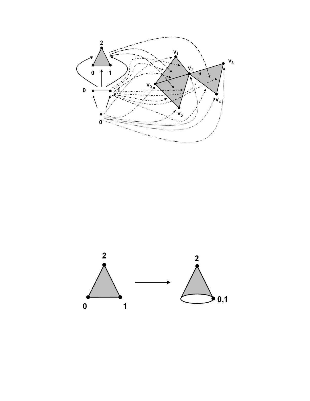
An elemen tary illustrated in tro duction to simplicial sets Greg F riedman T exas Christian Univ ersit y Decem b er 6, 2011 (minor corrections August 13, 2015; Octob er 3, 2016; Decem b er 21, 2020; Ma y 25, 2021; June 10, 2022; and June 8, 2023 — see errata at end of pap er) 2000 Mathematics Sub ject Classiﬁcation: 18G30, 55U10 Keyw ords: Simplicial sets, simplicial homotop y Abstract This is an exp ository in tro duction to simplicial sets and simplicial homotop y the- ory with particular fo cus on relating the combinatorial aspects of the theory to their geometric/top ological origins. It is in tended to be accessible to studen ts familiar with just the fundamen tals of algebraic top ology . Con ten ts 1 In tro duction 2 2 A build-up to simplicial sets 3 2.1 Simplicial complexes . . . . . . . . . . . . . . . . . . . . . . . . . . . . . . . 3 2.2 Simplicial maps . . . . . . . . . . . . . . . . . . . . . . . . . . . . . . . . . . 6 2.3 Ordered simplicial complexes and face maps . . . . . . . . . . . . . . . . . . 8 2.4 Delta sets and Delta maps . . . . . . . . . . . . . . . . . . . . . . . . . . . . 10 3 Simplicial sets and morphisms 15 4 Realization 24 5 Pro ducts 29 5.1 Simplicial Hom . . . . . . . . . . . . . . . . . . . . . . . . . . . . . . . . . . 34 6 Simplicial ob jects in other categories 35 7 Kan complexes 37 1 8 Simplicial homotopy 39 8.1 P aths and path comp onen ts . . . . . . . . . . . . . . . . . . . . . . . . . . . 40 8.2 Homotopies of maps . . . . . . . . . . . . . . . . . . . . . . . . . . . . . . . 42 8.3 Relativ e homotopy . . . . . . . . . . . . . . . . . . . . . . . . . . . . . . . . 44 9 π n ( X , ∗ ) 45 10 Concluding remarks 54 1 In tro duction The following notes grew out of m y own diﬃculties in attempting to learn the basics of sim- plicial sets and simplicial homotop y theory , and th us they are aimed at someone with roughly the same starting knowledge I had, sp eciﬁcally some amoun t of comfort with simplicial ho- mology and the basic fundamen tals of top ological homotop y theory , including homotop y groups. Equipp ed with this background, I w anted to understand a little of what simplicial sets and their generalizations to other categories are all ab out, as they seem ubiquitous in the literature of certain schools of top ology . T o name just a few imp ortan t instances of whic h I am a ware, simplicial ob jects o ccur in Ma y’s w ork on recognition principles for iter- ated lo op spaces [11], Quillen’s approach to rational homotopy theory (see [17, 6]), Bousﬁeld and Kan’s work on completions, localization, and limits in homotop y theory [1], Quillen’s abstract treatmen t of homotopy theory [18], and v arious asp ects of homological algebra, including group cohomology , Ho chsc hild homology , and cyclic homology (see [23]). Ho wev er, in attempting to learn the rudiments of simplicial theory , I encountered imme- diate and discouraging diﬃculties, whic h led to serious frustration on sev eral o ccasions. It w as only after several diﬀerent attempts from diﬀerent angles that I ﬁnally b egan to “see the picture,” and m y intended goal here is to aid future students (of all ages) to ease in to the sub ject. My initial diﬃcult y with the classic exp ository sources such as Ma y [12] and Curtis [3] w as the extent to whic h the theory is presen ted purely com binatorially . And the combinatorial deﬁnitions are not often pretty; they tend to consist of long strings of axiomatic conditions (see, for example, the com binatorial deﬁnition of simplicial homotop y , Deﬁnition 8.6, b elow). Despite simplicial ob jects originating in very top ological settings, these classic exp ositions often sw eep this fact to o far under the rug for m y taste, as someone who likes to comprehend ev en algebraic and combinatorial constructions as visually as p ossible. There is a little bit more geometry in Mo ore’s lecture notes [14], though still not muc h, and these are also more diﬃcult to obtain (at least not without some go o d help from a solid Interlibrary Loan Departmen t). On the other hand, there is a muc h more mo dern p oint of view that sw eeps b oth top ology and com binatorics a wa y in fa vor of axiomatic category theory! Goerss and Jardine [9] is an excellen t mo dern text based up on this approach, which, ironically , help ed me tremendously to understand what the com binatorics were getting at! So what are w e getting at here? My goal, still as someone v ery far from an exp ert in either com binatorial or axiomatic simplicial theory , is to revisit the material cov ered in, roughly , 2 the ﬁrst chapters (in some cases the ﬁrst few pages) of the texts cited ab o ve and to provide some concrete geometric signp osts. Here, for the most part, you w on’t ﬁnd many complete pro ofs of theorems, and so these notes will not b e completely self-contained. Rather, I try primarily to sho w b y example how the very basic com binatorics, including the deﬁnitions, arise out of geometric ideas and to show the geometric ideas underlying the most elementary pro ofs and prop erties. Think of this as an app endix or a set of fo otnotes to the ﬁrst chapters of the classic exp ositions, or p erhaps as a Chapter 0. This may not sound lik e m uch, but during my earliest learning stages with this material, I w ould ha ve b een very grateful for something of the sort. Theoretically my reader will acquire enough of “the idea” to go forth and read the more thorough (and more tec hnical) sources equipp ed with enough in tuition to se e what’s going on. In Section 2, we lay the groundw ork with a lo ok at the more familiar topics of simplicial sets and, their slight generalizations, Delta sets. Simplicial sets are then in tro duced in Section 3, follow ed b y their geometric realizations in Section 4 and a detailed lo ok at products of simplicial sets in Section 5. In Section 6, w e provide a brief lo ok at how the notion of simplicial sets is generalized to other kinds of simplicial ob jects based in diﬀerent categories. In Section 7, we introduce Kan complexes; these are the simplicial sets that lend themselv es to simplicial analogues of homotopy theory , whic h w e study in Section 8. This section gets a bit more tec hnical as we head to ward more serious applications and theorems in simplicial theory , including the deﬁnition and prop erties of the simplicial homotopy groups π n ( X , ∗ ) in Section 9. Finally , in Section 10, we make some concluding remarks and steer the reader to ward more comprehensive exp ository sources. Ac knowledmen ts. I thank Jim McClure for his useful suggestions and Efton Park for his careful reading of and commen ts on the preliminary man uscript. Later corrections and impro vemen ts were suggested b y Henry Adams, Daniel M ¨ ullner, Peter Landw eb er, and an anon ymous referee. I am very grateful for the amount of attention this exp osition has receiv ed since its initial p osting at . One text diagram in this pap er was t yp eset using the T E X comm utative diagrams pack age b y Paul T a ylor. 2 A build-up to simplicial sets W e b egin at the b eginning with the relev an t geometric notions and their immediate com bi- natorial coun terparts. 2.1 Simplicial complexes Simplicial sets are, essentially , generalizations of the geometric simplicial complexes of el- emen tary algebraic topology (in some cases quite extreme generalizations). So let’s recall simplicial complexes, referring the absolute b eginner to [15] for a complete course in the essen tials. 3 Recall that a (ge ometric) n -simplex is the con vex set spanned by n + 1 geometrically indep enden t p oints { v 0 , . . . , v n } in some euclidean space. Here “geometrically indep enden t” means that the collection of n vectors v 1 − v 0 , . . . , v n − v 0 is linearly indep enden t, and this implies that an n -simplex is homeomorphic to a closed n -dimensional ball. The p oints v i are called vertic es . A fac e of the (geometric) n -simplex determined b y { v 0 , . . . , v n } is the conv ex set spanned by some subset of these vertices. A (ge ometric) simplicial c omplex X in R N consists of a collection of simplices, p ossibly of v arious dimensions, in R N suc h that 1. every face of a simplex of X is in X , and 2. the intersection of an y tw o simplices of X , if non-empty , is a face of eac h them. This deﬁnition can b e extended easily to handle geometric simplicial complexes containing collections of simplices of arbitrary cardinalit y and n -simplices for arbitrary non-negativ e in teger n . Since w e will head directly to ward abstractions that will ob viate this issue by other means, we refer the interested reader to [15, Section 2]. W e also observe that one is often in terested in a geometric simplicial complex only for its homeomorphism type and its combinatorial information, in whic h case one tends to ignore the precise em b edding in to euclidean space. This will b e the sense in whic h w e shall generally think of simplicial complexes. So, less formally , we think of a simplicial complex X as made up of simplices (generalized tetrahedra) of v arious dimensions, glued together along common faces (see Figure 1). The most eﬃcien t description, containing all of the relev ant information, comes from lab eling the v ertices (the 0-simplices) and then sp ecifying whic h collections of v ertices together constitute the v ertices of simplices of higher dimension. If the collection of vertices is coun table, we can lab el them v 0 , v 1 , v 2 , . . . , though this assumption is not strictly necessary - w e could lab el by { v i } i ∈ I for an y indexing set I . Then if some collection of v ertices { v i 0 , . . . , v i n } constitutes the v ertices of a simplex, we can lab el that simplex as [ v i 0 , . . . , v i n ]. Example 2.1 . If X is a complex and [ v i 0 , . . . , v i k ] is a simplex of X , then an y subset of { v i 0 , . . . , v i k } is a face of that simplex and thus itself a simplex of X . In particular, w e can think of the k -simplex [ v i 0 , . . . , v i k ] as a ge ometric simplicial c omplex consisting of itself and its faces. A nice wa y to organize the combinato rial information inv olved is to deﬁne the sk eleta X k , k = 0 , 1 , . . . , of a simplicial complex so that X k is the set of all k -simplices of X . Notice that, having lab eled our vertices so that X 0 = { v i } i ∈ I , we can think of each element of X k as a certain subset of X 0 of cardinality k + 1. A subset { v i 0 , . . . , v i k } ⊂ X 0 is an element of X k precisely if [ v i 0 , . . . , v i k ] is a k -dimensional simplex of X . T o describ e a geometric simplicial complex giv en its set of v ertices, it is enough to know whic h collections of vertices { v i 0 , . . . , v i k } corresp ond to simplices [ v i 0 , . . . , v i k ] of the simpli- cial complex. Paring do wn to this information (which is purely combinatorial) leads us to the notion of an abstr act simplicial c omplex . 4 Figure 1: A simplicial complex. Note that [ v 0 , v 1 , v 2 ] is a simplex, but [ v 1 , v 2 , v 4 ] is not. Deﬁnition 2.2. An abstr act simplicial c omplex consists of a set of “v ertices” X 0 together with, for each in teger k , a set X k consisting of subsets 1 of X 0 of cardinality k + 1. These m ust satisfy the condition that any ( j + 1)-elemen t subset of an element of X k is an elemen t of X j . Eac h elemen t of X k is an abstract k -simplex, and the last requiremen t of the deﬁnition just guarantees that ev ery face of an abstract simplex in an abstract simplicial complex is also a simplex of the simplicial complex. So, an abstract simplicial complex has exactly the same combinatorial information as a geometric simplicial complex. W e ha ve lost geometric information ab out how big a simplex is, how it is embedded in euclidean space, etc., but we ha ve retained all of the information necessary to reconstruct the complex up to homeomorphism. It is straigh tforward that a geometric simplicial complex yields an abstract simplicial complex, but conv ersely , we can obtain a geometric simplicial complex (up to homeomorphism) from an abstract one b y assigning to eac h elemen t of X 0 a p oint and to each abstract simplex [ v i 0 , . . . , v i k ] a geometric k -simplex spanned b y the appropriate vertices and gluing these simplices together via the quotient topology . This pro cess can b e carried out either concretely geometrically by c ho osing speciﬁc (and suﬃcien tly geometrically independent) p oin ts within some generalized euclidean space, or, as w e shall prefer to think of it, more purely top ologically b y c ho osing standard representativ e simplices of the homeomorphism t yp e of euclidean simplices and then gluing abstractly . It is w orth noting separately the imp ortant p oint that, just like for a geometric simpli- cial complex, a simplex in an abstract simplicial complex is completely determined b y its 1 Not necessarily all of them! 5 collection of vertices. 2.2 Simplicial maps The appropriate notion of a morphism betw een tw o geometric simplicial complexes is the simplicial map. Such maps will play an imp ortant role as we transition from simplicial complexes to simplicial sets. Recall (see [15, Section 2]) that if K and L are geometric simplicial complexes, then a simplicial map f : K → L is determined by taking the v ertices { v i } of K to vertices { f ( v i ) } of L suc h that if [ v i 0 , . . . , v i k ] is a simplex of K then f ( v i 0 ) , . . . , f ( v i k ) are all vertices (not necessarily unique) of some simplex in L . Given suc h a function K 0 → L 0 , the rest of f : K → L is determined b y linear in terp olation on eac h simplex (if x ∈ K can b e represen ted by x = P n j =1 t j v i j in barycen tric co ordinates of the simplex spanned b y the v i j , then f ( x ) = P n j =1 t j f ( v i j )). The resulting function f : K → L is con tinuous (see [15]). Example 2.3 . A simple, y et in teresting and imp ortant example, is the inclusion of an n - simplex into a simplicial complex (Figure 2). If X is a simplicial complex and v i 0 , . . . , v i n is a collection of vertices of X that spans an n -simplex of X , then K = [ v i 0 , . . . , v i n ] is itself a simplicial complex. W e then hav e a simplicial map K → X that takes each v i j to the corresp onding v ertex in X and hence takes K identically to itself inside X . Figure 2: Including the simplex [ v 2 , v 3 , v 4 ] in to a larger simplicial complex 6 Example 2.4 . Some other very interesting examples of simplicial maps, which will b e critical for our developmen t of simplicial sets, are the simplicial maps that collapse simplices. F or example, let [ v 0 , v 1 , v 2 ] b e a 2-simplex, one of whose 1-faces is [ v 0 , v 1 ]. Consider the simplicial map f : [ v 0 , v 1 , v 2 ] → [ v 0 , v 1 ] determined by f ( v 0 ) = v 0 , f ( v 1 ) = v 1 , f ( v 2 ) = v 1 that collapses the 2-simplex down to the 1-simplex (see Figure 3). The great b eneﬁt of the theory of simplicial sets is a wa y to generalize these kinds of maps in order to preserve information so that we can still see the image of the 2-simplex hiding in the 1-simplex as a de gener ate simplex (see Section 3). Figure 3: A collapse of a 2-simplex to a 1-simplex Of course simplicial maps of geometric simplicial complexes determine simplicial maps of abstract simplicial complexes by simply recording where eac h vertex of the domain go es. Con versely , observe that a simplicial map is describ ed entirely in terms of abstract simplicial complex information; it is determined completely b y sp ecifying an image vertex for eac h v ertex in the domain complex. F urthermore, once we ha v e simplicial maps, we ha ve a notion of simplicial homeomorphism, and this allows us once and for all to identify , up to simplicial homeomorphism, an abstract simplicial complex with all the geometric simplicial complexes that p ossess the same combinatorial data, all of whic h will b e simplicially homeomorphic to eac h other. This will justify our use b elo w of the phrase “simplicial complex”, from whic h w e may drop the w ord “geometric” or “abstract”. 7 2.3 Ordered simplicial complexes and face maps A sligh tly more sp eciﬁc wa y to do all this is to let the set of vertices X 0 of a simplicial complex X b e totally ordered, in whic h case we obtain an or der e d simplicial c omplex . When w e do this, the symbol [ v i 0 , . . . , v i k ] may stand for a simplex if and only if v i j < v i l whenev er j < l . This poses no undue complications as each collection { v i 0 , . . . , v i k } of cardinalit y k still corresp onds to at most one simplex. W e’re just b eing picky and removing some redundancy in ho w many w ays we can lab el a giv en simplex of a simplicial complex. Example 2.5 . The protot ypical example of an ordered simplicial complex is the (ordered) n -simplex itself 2 . The or der e d n -simplex is simply an n -simplex with ordered v ertices. It is an ordered simplicial complex when considered together with its faces as in Example 2.1. W e denote the ordered n -simplex | ∆ n | ; it will b ecome clear later wh y we w an t to emplo y the notation | ∆ n | instead of just ∆ n . The n -simplex is so fundamen tal that one often lab els the v ertices simply with the num b ers 0 , 1 , . . . , n , so that | ∆ n | = [0 , . . . , n ] (see Figure 4). Each k -face of | ∆ n | then has the form [ i 0 , . . . , i k ], where 0 ≤ i 0 < i 1 < . . . < i k ≤ n . Figure 4: The standard ordered 0-, 1-, 2-, and 3-simplices The notation [0 , . . . , n ] for the standard ordered n -simp ex should b e suggestiv e when compared with the simplices [ v i 0 , . . . , v i n ] app earing within more general ordered simplicial complexes, and it is w orth p ointing out at this early stage that one can think of any suc h simplex in a complex X as the image of | ∆ n | under a simplicial map (order-preserving) taking 0 to v i 0 , and so on. Since X is an ordered simplicial complex, then there is precisely one w ay to do this for eac h n -simplex of X . Th us another p oint of view on ordered simplicial complexes is that they are made up out of images of the standard ordered simplices (Figure 5). This will turn out to b e a v ery useful p oint of view as w e progress. F ace maps. Another asp ect of ordered simplicial complexes familiar to the studen t of basic algebraic top ology is that, given an n -simplex, w e would lik e a handy w a y of referring to its ( n − 1)-dimensional faces (its ( n − 1) -fac es ). This is handled b y the fac e maps . On 2 Notice that we hav e already b egun employing the abstraction promised at the end of the last section b y referring to the n -simplex. Of course, to b e tec hnical, the n -simplex refers to the (abstract or geometric) simplicial homeomorphism class, as there are many diﬀerent w ays to realize the n -simplex in euclidean space as a sp eciﬁc geometric n -simplex (though of course, up to relab eling, there is only one wa y to describe it as an abstract simplicial complex - which is sort of the p oint of introducing abstract simplicial complexes in the ﬁrst place). 8 Figure 5: [ v 2 , v 3 , v 4 ] as the image of | ∆ 2 | the standard n -simplex, w e hav e n + 1 face maps d 0 , . . . , d n , deﬁned so that d j [0 , . . . , n ] = [0 , . . . , ˆ , . . . , n ], where, as usual, the ˆ denotes a term that is b eing omitted. Th us applying d j to [0 , . . . , n ] yields the ( n − 1)-face missing the v ertex j (see Figure 6). It is imp ortan t to note that each d j simply assigns to the n -simplex one of its faces; there is no underlying p oin t-set top ological or simplicial map meant. Figure 6: The face maps of | ∆ 2 | . Note w ell: the arrows denote assignments , not contin uous maps of spaces. Within more general ordered simplicial complexes, we make the obvious extension: if [ v i 0 , . . . , v i n ] ∈ X n is a simplex of the complex X , then d j [ v i 0 , . . . , v i n ] = [ v i 0 , . . . , ˆ v i j , . . . , v i n ]. 9 Assem bled all together, w e get, for eac h ﬁxed n , a collection of functions d 0 , . . . , d n : X n → X n − 1 . Note that here is where the ordering of the vertices of the simplices b ecomes imp or- tan t. If one w anted to b e a serious stic kler, we might b e careful to lab el the face maps from X n to X n − 1 as d n 0 , . . . , d n n , but this is rarely done in practice, for whic h we should probably b e grateful. Th us d j is used to represent the face map leaving out the j th v ertex in any dimension where this makes sense (i.e. dimensions ≥ j ). F urthermore, one readily sees by playing with | ∆ n | that there are certain relations satis- ﬁed b y the face maps. In particular, if i < j , then d i d j = d j − 1 d i . (1) Indeed, d i d j [0 , . . . , n ] = [0 , . . . , ˆ ı, . . . , ˆ , . . . , n ] = d j − 1 d i [0 , . . . , n ] (notice the reason that we ha ve d j − 1 in the last expression is that remo ving the i ﬁrst shifts the j in to the j − 1 slot). Clearly , the relation d i d j = d j − 1 d i m ust hold for any simplex in a complex X (which is made up of copies of | ∆ n | ). This relation will b ecome one of the axioms in the deﬁnition of a simplicial set when we get there. Another observ ation that will come up later is that there are more general face maps. W e could, for example, assign to [0 , 1 , 2 , 3 , 4 , 5 , 6] the face [1 , 3 , 4], and we could deﬁne suc h general face maps systematically . Ho w ever, any such face can b e obtained as a comp osition of face maps that low er dimension b y 1. F or example, we can decomp ose the map just describ ed as d 0 d 2 d 5 d 6 . It may entertain the reader to use the “face map relations” and some basic reasoning to sho w that any generalized face map can b e obtained as a comp osition d i 1 · · · d i m uniquely if we require that i j < i j +1 for all j . 2.4 Delta sets and Delta maps Delta sets (sometimes called ∆-sets) constitute an in termediary b et w een simplicial com- plexes and simplicial sets. These allow a degree of abstraction without yet in tro ducing the degeneracy maps we hav e b egun hin ting at. Deﬁnition 2.6. A Delta set 3 consists of a sequence of sets X 0 , X 1 , . . . and, for eac h n ≥ 0, maps d i : X n +1 → X n for eac h i , 0 ≤ i ≤ n + 1, suc h that d i d j = d j − 1 d i whenev er i < j . Of course this is just an abstraction, and generalization, of the deﬁnition of an ordered simplicial complex, in whic h the X n are the sets of n -simplices and the d i are the face maps. Ho wev er, there are Delta sets that are not simplicial complexes: Example 2.7 . Consider the cone C obtained by starting with the standard ordered 2-simplex | ∆ 2 | = [0 , 1 , 2] and gluing the edge [0 , 2] to the edge [1 , 2] (see Figure 7). This space is no longer a simplicial complex (at least not with the “triangulation” giv en), since in a simplicial complex, the faces of a giv en simplex must b e unique. This is no longer the case here as, for example, the “edge [0,1]” now has b oth endp oin t vertices equal to eac h other. 3 It seems to b e at least fairly usual to capitalize the word “Delta” in this context, probably b ecause it is essentially a stand-in for the Greek capital letter ∆. Ho wev er, for reasons that will become clear, it is probably best to av oid the notation “∆-set” and to use instead the English stand-in. 10 Figure 7: Gluing | ∆ 2 | in to a cone Ho wev er, this is a Delta set. Without (I hop e!) to o muc h risk of confusion, w e use the notation for the simplices in the triangle to refer also to their images in the cone. So, for example [0] and [1] now b oth stand for the same vertex in the cone and [0 , 1] stands for the circular base edge. Then C 0 = { [0] , [2] } , C 1 = { [0 , 1] , [0 , 2] } , C 2 = [0 , 1 , 2], and C n = ∅ for all n > 2. The face maps are the obvious ones, also induced from the triangle, so that, e.g. d 2 [0 , 1 , 2] = [0 , 1] and d 0 [0 , 1] = d 1 [0 , 1] = [0] = [1]. It is not hard to see that the face map relation (1) is satisﬁed - it comes right from the fact that it holds for the standard 2-simplex. Example 2.8 . One feature of Delta sets we need to b e careful ab out is that, unlike for simplicial complexes, a collection of v ertices do es not necessarily sp ecify a unique simplex. F or example, consider the Delta set with X 0 = { v 0 , v 1 } , X 1 = { e 0 , e 1 } , d 0 ( e 0 ) = d 0 ( e 1 ) = v 0 , and d 1 ( e 0 ) = d 1 ( e 1 ) = v 1 . Both 1-simplices ha ve the same endp oin ts. See Figure 8. Figure 8: A Delta set containing tw o edges with the same v ertices Th us Delta sets aﬀord some greater ﬂexibility b ey ond ordered simplicial complexes. One ma y con tinue to think of the sets X n as collections of simplices and in terpret from the face maps ho w these are meant to b e glued together (Exercise: Giv e each “simplex” of the cone X of the preceding example an abstract lab el, write out the full set of face maps in these lab els, then reverse engineer how to construct the cone from this information. One sees that ev erything is forced. F or example, there is one 2-simplex, tw o of whose faces are the same, so they m ust b e glued together!). Ho wev er, it is common in the fancier literature not to think of the X n as collections of simplices at all but simply as abstract sets with abstract collections of face maps. At least this is what authors w ould hav e us b eliev e - I tend to picture simplices in m y head anyw ay , while k eeping in mind that this is more of a cognitive aid than it is “what’s really going on.” 11 The category-theoretic deﬁnition. While w e’re walking the tightrope of abstraction, let’s take it a step further. Recall that w e discussed in Example 2.5 that we can think of an ordered simplicial complex as a collection of isomorphic images of the standard n -simplices (for v arious n ). Of course to describ e the simplicial complex fully we need to kno w not just ab out these copies of the standard simplices but also ab out ho w their faces are attac hed together. This information is con tained in the face maps, which tell us when tw o simplices share a face. There’s an alternative deﬁnition of Delta complexes that takes more of this p oin t of view. It migh t b e a little scary if you’re not that comfortable with category theory , but don’t w orry , I’ll walk you through it (though I do assume you know the basic language of categories and functors). First, w e deﬁne a category b ∆: Deﬁnition 2.9. The category b ∆ has as ob jects the ﬁnite ordered sets [ n ] = { 0 , 1 , 2 . . . , n } . The morphisms of b ∆ are the strictly order-preserving functions [ m ] → [ n ] (recall that f is strictly order-preserving if i < j implies f ( i ) < f ( j )). The ob jects of b ∆ should b e thought of as our prototype or der e d n -simplices. The mor- phisms are only deﬁned when m ≤ n , and y ou can think of these morphisms as taking an m -simplex and embedding it as a face of an n -simplex (see Figure 9). Note that, since order matters, there are exactly as man y w ays to do this as there are strictly order-preserving maps [ m ] → [ n ]. Next, w e think ab out the opp osite category b ∆ op . Recall that this means that we keep the same ob jects [ n ] of b ∆, but for every morphism [ m ] → [ n ] in b ∆, w e instead ha ve a map [ n ] → [ m ] in b ∆ op . What should this mean? W ell if a giv en morphism [ m ] → [ n ] w as the inclusion of a face, then the new opp osite map [ n ] → [ m ] should b e thought of as taking the n -simplex [ n ] and prescribing a given face. This is just a generalization of what we ha ve seen already: if w e consider in b ∆ the morphism D i : [ n ] → [ n + 1] deﬁned by the strictly order- preserving map { 0 , . . . , n } → { 0 , . . . , ˆ ı, . . . , n + 1 } , then in b ∆ op this corresp onds precisely to the simplex face map d i . Ev en b etter, it is easy to c hec k once again t hat, with this deﬁnition, d i d j = d j − 1 d i when i < j , simply as an eviden t property of strictly order-preserving maps. This is really how we argued for this axiom in the ﬁrst place! So, in summary , the category b ∆ op is just the collect ion of elemen tary n -simplices together with the face maps (satisfying the face map axiom) and the iterations of face maps. But this should b e precisely the protot yp e for all Delta sets: Deﬁnition 2.10 (Alternative deﬁnition for Delta sets) . A Delta set is a cov ariant functor X : b ∆ op → Set , where Set is the category of sets and functions. Equiv alen tly , a Delta set is a con trav arian t functor b ∆ → Set . Let’s see wh y this mak es sense. A functor tak es ob jects to ob jects and morphisms to morphisms, and it ob eys composition rules. So, un winding the deﬁnition, a co v ariant functor b ∆ op → Set assigns to [ n ] ∈ b ∆ op a set X n (whic h we can think of, and which we refer to, as a set of simplices) and giv es us, for eac h strictly order-preserving [ m ] → [ n ] in b ∆ (or its corresponding opp osite in b ∆ op ) a generalized face map X n → X m (whic h we think of as assigning an m -face to eac h simplex in X n ). As noted previously , these generalized face 12 Figure 9: A partial illustration of the category b ∆ maps are all comp ositions of our standard face maps d i , so the d i (and their axioms) are the only ones we usually b other fo cusing on. So what just happened? The p o wer of this deﬁnition is really in its point of view. Instead of thinking of a Delta set as b eing made up of a whole bunc h of simplices one at a time, w e can now think of the standard n -simplex as standing for all of the simplices in X n , all at once - the functor X assigns to [ n ] the collection of all of the simplices of X n (see Figure 10). The face map d i applied to the standard simplex [ n ] represents all of the i th faces of all the n -simplices simultaneously . A t the same time, w e see how an y argumen t in X really comes from what happ ens back in b ∆. The axiom d i d j = d j − 1 d i in a Delta set X is just a consequence of this b eing true in the prototype simplex [ n ] and inherent prop erties of functors. W e’ll get a lot of mileage out of this kind of thinking: things w e’d lik e to prov e in a Delta set X can often b e pro ved just b y proving them in the prototype standard simplex and applying functorialit y . 13 Figure 10: A Delta complex as the functorial image of b ∆ Delta maps. W e won’t dw ell ov erly long on Delta maps, except to observ e that they , to o, p oin t to w ard the need for simplicial sets (how ev er, see [19] where Delta complexes and Delta maps are treated in their o wn right). Going directly to the category theoretic deﬁnition, given tw o Delta sets X , Y , though t of as con trav ariant functors b ∆ → Set , a morphism X → Y is a natural transformation of functors from X to Y . In other w ords, a morphism consists of a collection of set maps X n → Y n that comm ute with the face maps. Example 2.11 . There is an evident Delta map from the standard 2-simplex [0 , 1 , 2] to the cone C of Example 2.7. See Figure 11. Figure 11: The Delta map from | ∆ 2 | to the cone The astute reader will notice something ﬁshy here. W e would hop e that simplicial maps of simplicial complexes would yield morphisms of Delta sets. How ever, consider the collapse π : | ∆ 2 | = [0 , 1 , 2] → | ∆ 1 | = [0 , 1] deﬁned by π (0) = 0 and π (1) = π (2) = 1 (see Figure 3). T o b e a Delta set morphism, the simplex [0 , 1 , 2] ∈ | ∆ 2 | 2 w ould hav e to b e tak en to 14 an element of | ∆ 1 | 2 . But this set is empty! There are no 2-simplices of | ∆ 1 | . Something is amiss. W e need simplicial sets. 3 Simplicial sets and morphisms Simplicial sets generalize b oth simplicial complexes and Delta sets. When approaching the literature, the reader should b e very careful ab out terminology . Originally ([5]), Delta sets were referred to as semi-simplicial c omplexes , and, once the degeneracy op erations we are ab out to discuss w ere discov ered, the term c omplete semi- simplicial c omplex ( c.s.s. set , for short) w as in tro duced. Over time, with Delta sets b ecoming of less in terest, “complete semi-simplicial” was abbreviated bac k to “semi-simplicial” and ev entually to “simplicial,” lea ving us with the simplicial sets of today . Meanwhile, some mo dern authors hav e returned to using “semi-simplicial complexes” to refer to what w e are calling Delta sets, on the grounds that, as we will see, the category ∆ (“Delta”) is the protot yp e for simplicial sets, not Delta sets, for whic h w e ha ve b een using the protot yp e category b ∆. This all sounds v ery confusing b ecause it is, and the reader is advised to b e v ery careful when reading the literature. 4 W e try to b e careful and use only the three terms “simplicial complex,” “Delta set,” and “simplicial set.” In particular, b e sure to note the diﬀerence b etw een “simplicial complex” and “simplicial set” going forward. Degenerate simplices. Recall from Example 2.4 that a simplicial map can collapse a simplex. In that example, w e had a simplicial map π : | ∆ 2 | → | ∆ 1 | deﬁned on vertices so that π (0) = 0 and π (1) = π (2) = 1. Recall also that w e ha ve begun to think of simplicial complexes and Delta sets as collections of images of standard simplices under appropriate maps. W ell, here is a map of the standard 2-simplex | ∆ 2 | . What image simplex do es it giv e us in | ∆ 1 | under π ? In the land of simplicial sets, the image π ( | ∆ 2 | ) is an example of a de gener ate simplex. Roughly sp eaking, degenerate simplices are simplices that don’t ha ve the “correct” n umber of dimensions. A degenerate 3-simplex migh t b e realized geometrically as a 2- dimensional, 1-dimensional, or 0-dimensional ob ject. Geometrically , degenerate simplices are “hidden”; thus the clearest approach to dealing with them lies in the combinatorial notation w e hav e b een dev eloping all along. The k ey b oth to the idea and to the notation is in allowing vertices to repeat. The natural w ay to lab el π ( | ∆ 2 | ) = π ([0 , 1 , 2]) in our example is as [0 , 1 , 1], reﬂecting where the vertices of | ∆ 2 | go under the map. This violates our earlier principle that simplices in complexes should b e written [ v 0 , . . . , v n ] with the v i distinct vertices written in order, but sometimes in mathematics w e need a new, more general principle. F or degenerate simplices, we’ll k eep the orderings but disp ense with the uniqueness. Thus, oﬃcially , a de gener ate simplex is a [ v i 0 , . . . , v i n ] for which the v i j are not all distinct, though we do still require i k ≤ i ℓ if k <  . 4 I thank Jim McClure for explaining to me this historical progression. 15 Example 3.1 . How man y 1-simplices, including degenerate ones, are lurking within the ele- men tary 2-simplex [0 , 1 , 2]? A 1-simplex is still written [ a, b ], with a ≤ b , but now rep etition is allo wed. The answ er is six: [0 , 1], [0 , 2], [1 , 2], [0 , 0], [1 , 1], and [2 , 2]. See the middle picture in Figure 12. Similarly , within | ∆ 2 | = [0 , 1 , 2] there are now three kinds of 2-simplices. W e ha ve the nondegenerate [0 , 1 , 2], the 2-simplices that degenerate to 1-dimension such as [0 , 1 , 1] and [0 , 0 , 2], and w e ha ve the 2-simplices that degenerate to 0-dimensions suc h as [0 , 0 , 0] and [2 , 2 , 2]. W orking with degenerate simplices makes dra wing diagrams muc h more diﬃcult. W e tak e a crack at it in Figure 12. As implied b y the diagram, w e can think of degenerate simplices as b eing the images of collapsing maps such as that in Example 2.4. Of course an y simplicial complex or Delta set can b e expanded conceptually to include degenerate simplices. In the example of Figure 1, w e might hav e the degenerate 5-simplex [ v 2 , v 2 , v 2 , v 3 , v 3 ]. Notice also that our inno cen t little n -dimensional simplicial complexes suddenly con tain degenerate simplices of arbitrarily large dimension. Even the 0-simplex | ∆ 0 | = [0] b ecomes host to degenerate simplices such as [0 , 0 , 0 , 0 , 0 , 0 , 0 , 0 , 0 , 0 , 0 , 0 , 0 , 0 , 0 , 0 , 0 , 0]. The situation has degenerated indeed! T o k eep trac k of it all, we need de gener acy maps . Degeneracy maps. Degeneracy maps are, in some sense, the conceptual conv erse of face maps. Recall that the face map d j tak es an n -simplex and giv e us back its j th ( n − 1)-face. On the other hand, the j th degeneracy map s j tak es an n -simplex and gives us bac k the j th degenerate ( n + 1)-simplex living inside it. As usual, we illustrate with the standard n -simplex, whic h will b e a mo del for what happ ens in all simplicial sets. Giv en the standard n -simplex | ∆ n | = [0 , . . . , n ], there are n + 1 degeneracy maps s 0 , . . . , s n , deﬁned by s j [0 , . . . , n ] = [0 , . . . , j, j , . . . , n ]. In other w ords, s j [0 , . . . , n ] gives us the unique degenerate n + 1 simplex in | ∆ n | with only the j th v ertex rep eated. Again, the geometric concept is that s j | ∆ n | can be thought of as the pro cess of collapsing ∆ n +1 do wn in to ∆ n b y the simplicial map π j deﬁned by π j ( i ) = i for i < j , π j ( j ) = π j ( j + 1) = j and π j ( i ) = i − 1 for i > j + 1. This idea extends naturally to simplicial complexes, to Delta sets, and to simplices that are already degenerate. If we ha v e a (p ossibly degenerate) n -simplex [ v i 0 , . . . , v i n ] with i k ≤ i k +1 for eac h k , 0 ≤ k < n , then w e set s j [ v i 0 , . . . , v i n ] = [ v i 0 , . . . , v i j , v i j , . . . , v i n ], i.e. rep eat v i j . This is a degenerate simplex in [ v i 0 , . . . , v i n ]. It is not hard to see that any degenerate simplex can b e obtained from an ordinary simplex by repeated application of degeneracy maps. Th us, just as any face of a simplex can b e obtained by using comp ositions of the d i , an y degenerate simplex can b e obtained from comp ositions of the s i . Also, as for the d i , there are certain natural relations that the degeneracy maps p ossess. In particular, if i ≤ j , then s i s j [0 , . . . , n ] = [0 , . . . , i, i, . . . , j, j, . . . , n ] = s j +1 s i [0 , . . . , n ]. Note 16 Figure 12: The ﬁrst picture represents all of the 1-simplices i n | ∆ 1 | , including the degenerate ones that are taken to individual vertices. The second picture represents all the 1-simplices in | ∆ 2 | , and the last picture represen ts all of the degenerate 2-simplices in | ∆ 2 | . 17 that we hav e s j +1 in the last form ula, not s j , since the application of s i pushes j one slot to the righ t. F urthermore, there are relations amongst the face and degeneracy op erators. These are a little more awkw ard to write down since there are three p ossibilities: d i s j = s j − 1 d i if i < j , d j s j = d j +1 s j = id , d i s j = s j d i − 1 if i > j + 1 . These can all b e seen rather directly . F or example, applying either side of the ﬁrst form ula to [0 , . . . , n ] yields [0 , . . . , ˆ ı, . . . , j, j, . . . , n ]. Note also that the middle form ula tak es care of b oth i = j and i = j + 1. Simplicial sets. W e are ﬁnally ready for the deﬁnition of simplicial sets: Deﬁnition 3.2. A simplicial set consists of a sequence of sets X 0 , X 1 , . . . and, for each n ≥ 0, functions d i : X n → X n − 1 and s i : X n → X n +1 for eac h i with 0 ≤ i ≤ n such that d i d j = d j − 1 d i if i < j , d i s j = s j − 1 d i if i < j , d j s j = d j +1 s j = id , (2) d i s j = s j d i − 1 if i > j + 1 , s i s j = s j +1 s i if i ≤ j . Example 3.3 . Our ﬁrst example is the critical observ ation that every ordered simplicial complex can b e made in to a simplicial set by adjoining all p ossible degenerate simplices. More precisely , supp ose X is an ordered simplicial complex. Then we obtain a simplicial set 5 ¯ X such that ¯ X n consists of all the simplices [ v i 0 , . . . , v i n ] where v i k ≤ v i k +1 and the set of vertices { v i 0 , . . . , v i n } spans a simplex of X ; note that the v i j are not required to b e unique. Another w a y to say this is that for ev ery simplex [ v i 0 , . . . , v i m ] of X , w e hav e in ¯ X all simplices of the form [ v i 0 , . . . , v i 0 , v i 1 , . . . , v i 1 , . . . , v i m ] for an y num b er of rep etitions of eac h of the vertices. The face and degeneracy maps are deﬁned on these simplices in the eviden t w ays. Similarly , every Delta set can b e “completed” to a simplicial set by an analogous pro cess, though some additional care is necessary as we know that an elemen t of a Delta set is not necessarily determined b y its vertices; we leav e the precise construction as an exercise for the reader. Con versely , each simplicial set yields a Delta set by neglect of structure (throw a wa y the degeneracy maps). How ever, a simplicial set do es not necessarily come from an ordered simplicial complex by the pro cess describ ed ab ov e as, for example, not every Delta set is an ordered simplicial complex. 5 The notation transition X to ¯ X from an ordered simplicial complex to a simplicial set is not standard notation; w e simply use it for exp ediency in this example. 18 Example 3.4 . The standard 0-simplex X = [0], no w though t of as a simplicial set, is the unique simplicial set with one elemen t in each X n , n ≥ 0. The element in dimension n is n +1 times z }| { [0 , . . . , 0]. Example 3.5 . As a simplicial set, the standard ordered 1-simplex X = [0 , 1] already has n + 2 elemen ts in each X n . F or example, X 2 = { [0 , 0 , 0] , [0 , 0 , 1] , [0 , 1 , 1] , [1 , 1 , 1] } . R emark 3.6 . W e will use ∆ n or [0 , . . . , n ] to refer to the standard ordered n -simplex, thought of as a simplicial set. Example 3.7 . Now for an example familiar from algebraic top ology . Giv en a top ological space X , let S ( X ) n b e the set of contin uous functions from | ∆ n | to X . T ogether with face and degeneracy maps that we will describ e in a moment, these constitute a simplicial set called the singular set of X . The singular chain complex S ∗ ( X ) from algebraic top ology has eac h S n ( X ) equal to the free ab elian group generated by S ( X ) n . T o deﬁne the face and degeneracy maps, let σ : | ∆ n | → X b e a con tin uous map represen t- ing a singular simplex (Figure 13). The singular simplex d i σ is deﬁned as the restriction of σ to the i th face of | ∆ n | . Equiv alen tly it is the comp osition of σ and the simplicial inclusion map [0 , . . . , n − 1] → [0 , . . . , ˆ ı, . . . , n ] (Figure 14). These are precisely the same as the terms that sho w up in the b oundary map of the singular c hain complex where ∂ = P n i =0 ( − 1) i d i . Figure 13: A singular simplex On the other hand, the degeneracy s i tak es the singular simplex σ to the comp osition of σ : | ∆ n | = [0 , . . . , n ] → X with the geometric collapse represented by the degeneracy [0 , . . . , n + 1] → [0 , . . . , i, i, . . . , n ]. Once again, a degenerate simplex is a collapsed version of another simplex (Figure 15). 19 Figure 14: A face of a singular simplex Figure 15: A degenerate singular simplex 20 S ( X ) turns out to b e simplicial set, and w e invite the reader to think through why the relations (2) hold as a consequence of their holding for the standard ordered simplex. In some sense, this is our usual mo del, just redesigned within the con text of the contin uous map σ . Some more examples of simplicial sets are giv en b elow in Section 4, where w e can b etter study their geometric manifestations. Nondegenerate simplices. Deﬁnition 3.8. A simplex x ∈ X n is called nonde gener ate if x cannot b e written as s i y for an y y ∈ X n − 1 and an y i . Ev ery simplex in the sense of Section 2 of a simplicial complex or Delta set is a nondegen- erate simplex of the corresp onding simplicial set. If Y is a top ological space, an n -simplex of S ( Y ) is nondegenerate if it cannot b e written as the comp osition ∆ n π → ∆ k σ → Y , where π is a simplicial collapse with k < n and σ is a singular k -simplex. Note that it is p ossible for a nondegenerate simplex to hav e a degenerate face (see Exam- ple 4.7, b elow, though it might b e go o d practice to try to come up with your own example ﬁrst). It is also p ossible for a degenerate simplex to ha ve a nondegenerate face (for example, w e know d j s j x = x for any x , degenerate or not). The categorical deﬁnition. As for Delta sets, the basic prop erties of simplicial sets deriv e from those of the standard ordered n -simplex. In fact, that is where the prototypes of b oth the face and degeneracy maps live and where w e ﬁrst developed the axioms relating them. Th us it is not surprising (at this p oint) that there is a categorical deﬁnition of simplicial sets, analogous to the one for Delta sets, in which each simplicial set is the functorial image of a category , ∆, built from the standard simplices. Deﬁnition 3.9. The category ∆ has as ob jects the ﬁnite ordered sets [ n ] = { 0 , 1 , 2 . . . , n } . The morphisms of ∆ are order-preserving functions [ m ] → [ n ]. Notice that the only diﬀerence b etw een the deﬁnitions of b ∆ and ∆ is that the morphisms in ∆ only need to b e order-preserving and not strictly order-preserving. Th us, equating the ob jects [ n ] with the ordered simplices ∆ n , the morphisms no longer need to represent only inclusions of simplices but may represent degeneracies as well. In more familiar notation, a t ypical morphism, sa y , f : [5] → [3] migh t b e describ ed by f [0 , 1 , 2 , 3 , 4 , 5] = [0 , 0 , 2 , 2 , 2 , 3], whic h can b e though t of as a simplicial complex map taking the 5-simplex degenerately to the 2-face of the 3-simplex spanned b y 0, 2, and 3. As in b ∆, the morphisms in ∆ are generated b y certain maps b et ween neighboring car- dinalities D i : [ n ] → [ n + 1] and S i : [ n + 1] → [ n ], 0 ≤ i ≤ n . The D i are just as for b ∆: D i [0 , . . . , n ] = [0 , . . . , ˆ ı, . . . , n + 1]. The new maps, which couldn’t exist in b ∆, are deﬁned b y S i [0 , . . . , n + 1] = [0 , . . . , i, i, . . . , n ]. It is an easy exercise to verify that all morphisms in ∆ are comp ositions of the D i and S i and that these satisfy axioms analogous to those in the 21 deﬁnition of simplicial set. Later on, w e will also use D i and S i to stand for the geometric maps they induce on the standard geometric simplices. T o get to our categorical deﬁnition of simplicial sets, w e must, as for Delta sets, consider ∆ op . The maps D i b ecome their opp osites, denoted d i , and these corresp ond to the face maps as b efore: the opp osite of the inclusion D i : [ n ] → [ n + 1] of the i th face is the i th face map, d i , whic h assigns to the n -simplex its i th face. The opp osites of the S i b ecome the degeneracies; the opp osite of the collapse S i : [ n + 1] → [ n ] that pinc hes together the i -th and i + 1-th vertices of an n + 1 simplex is the i th degeneracy map, s i , whic h assigns to the n -simplex ∆ n the degenerate n + 1-simplex within ∆ n that rep eats the i th vertex. See Figure 16. Figure 16: How to visualize D i , d i , S i , and s i . Our diﬃculty with drawing degeneracies extends here so that we represen t the image of s i pictorially b y the picture for S i . In other w ords, the image of s 1 in the b ottom right is the degenerate 2-simplex arising from the collapse map S 1 . Of course, one can chec k that the d i and s i satisfy the axioms in the deﬁnition of simplicial set giv en ab ov e. Deﬁnition 3.10 (Categorical deﬁnition of simplicial set) . A simplicial set is a con trav ariant functor X : ∆ → Set (equiv alen tly , a co v ariant functor X : ∆ op → Set ). The reader should compare this with the categorical deﬁnition of Delta sets and reassure himself/herself that this deﬁnition is equiv alen t to Deﬁnition 3.2. As for Delta sets, the p o w er in this deﬁnition is that w e can think of the standard ordered n -simplex as standing for all of the simplices in X n , all at once - the functor X assigns to [ n ] all of the n -simplices in X n - and the standard face and degeneracy maps d i and s i pic k out all of the faces and degeneracies of X n b y functoriality . Example 3.11 . Let’s re-examine the singular set S ( Y ) of the top ological space Y from this p oin t of view. The singular set S ( Y ) is a functor ∆ → Set that assigns to [ n ] the set 22 Hom T op ( | ∆ n | , Y ), the set of all contin uous maps from | ∆ n | to Y . It assigns to the face and degeneracy maps of ∆ the face and degeneracy maps of Example 3.7, i.e. w e ha v e the follo wing corresp ondences: [ n ] Hom T op ( | ∆ n | , Y ) [ n ] Hom T op ( | ∆ n | , Y ) ⇒ ⇒ [ n − 1] d i ? Hom T op ( | ∆ n − 1 | , Y ) d i ? [ n + 1] s i ? Hom T op ( | ∆ n +1 | , Y ) . s i ? The reader should c hec k that the deﬁnitions for the face and degeneracy maps of the singular set deﬁned ab ov e are consistent with the claimed functorialit y . (Notice that the maps on the righ t sides of these diagrams should more appropriately b e lab eled S ( Y )( d i ) and S ( Y )( s i ), but we stic k with common practice and use d i and s i for face and degeneracy maps wherever w e ﬁnd them.) Simplicial morphisms. Simplicial sets themselves constitute a category S . The mor- phisms in this category are the simplicial morphisms : Deﬁnition 3.12. If X and Y are simplicial sets (and thus functors X , Y : ∆ → Set ), then a simplicial morphism f : X → Y is a natural transformation of these functors. Un winding this to more concrete language, f consists of set maps f n : X n → Y n that comm ute with face op erators and with degeneracy op erators. Example 3.13 . At last we ha ve a context in whic h to explore prop erly the collapse map π : | ∆ 2 | → | ∆ 1 | of Example 2.4. W e can extend π to a morphism of simplicial sets π : ∆ 2 → ∆ 1 b y prescribing π (0) = 0 and π (1) = π (2) = 1. Then as in Example 2.4, ∆ 2 = [0 , 1 , 2] is tak en to the degenerate simplex [0 , 1 , 1] = s 1 ([0 , 1]). A t the same time, the morphism π is doing an inﬁnite num b er of other things: it tak es the vertex [0] ∈ ∆ 2 to [0] ∈ ∆ 1 , it takes the vertices [1] , [2] ∈ ∆ 2 to [1] ∈ ∆ 1 , it tak es the 1-simplex [0 , 1] ∈ ∆ 2 to [0 , 1] ∈ ∆ 1 , it tak es the 1-simplex [1 , 2] ∈ ∆ 2 to the degenerate 1-simplex 6 [1 , 1] = s 0 [1] ∈ ∆ 1 , and it ev en tak es the degenerate simplex [0 , 1 , 1 , 2 , 2 , 2] = s 4 s 3 s 1 [0 , 1 , 2] ∈ ∆ 2 to the degenerate simplex s 4 s 3 s 1 [0 , 1 , 1] = [0 , 1 , 1 , 1 , 1 , 1] ∈ ∆ 1 . And m uc h muc h more. Example 3.14 . Notice that, unlik e simplicial maps on simplicial complexes, morphisms on simplicial sets are not completely determined b y what happens on v ertices. F or example, consider the p ossible simplicial morphisms from ∆ 1 to the simplicial set corresponding to the Delta set of Example 2.8. If w e ha ve a simplicial morphism that tak es [0] to [ v 0 ] and [1] to [ v 1 ], there are still tw o p ossibilities for where to send [0 , 1]. Example 3.15 . On the other hand, giv en a map of ordered simplicial complexes f : X → Y , this induces a map of the asso ciated simplicial sets as constructed in Example 3.3. In this case, a function on v ertices do es determine a simplicial map b ecause simplices of ordered 6 Careful: [1] is a 0-simplex, so s 0 is the appropriate (indeed the only w ell-deﬁned) degeneracy map. Remem b er that s 0 tells us to repeat what o ccurs in the 0th place - it do esn’t know what’s in that place. 23 simplicial complexes are determined uniquely b y their vertices. This was the case for the simplicial morphism of Example 3.13. R emark 3.16 . Notice that it is alw ays enough to deﬁne a simplicial morphism b y what it do es to nondegenerate simplices. What happ ens to the degenerate simplices is forced by the deﬁnition since, e.g. f ( s i ( x )) = s i ( f ( x )). Similarly , what happ ens on faces is forced b y what happ ens on the simplices of whic h they are faces. Thus, altogether, simplicial morphisms can b e described b y specifying what they do to a comparativ ely small collection of nondegenerate simplices. F rom here on, w e’ll abandon the distinction betw een “simplicial map” and “simplicial morphism” and use the terms in terchangeably as applied to simplicial sets. 4 Realization If the idea of simplicial ob jects is to abstract from geometry/top ology to com binatorics, there should b e a w ay to reverse that pro cess and turn simplicial sets in to geometric/top ological ob jects. Indeed that is the case. The deﬁnition lo oks a bit oﬀ-putting at ﬁrst (what con- cerning simplicial sets doesn’t?), but, in fact, w e’ll see that simplicial realization is a v ery natural thing to do. Deﬁnition 4.1. Let X b e a simplicial set. Giv e each set X n the discrete top ology and let | ∆ n | b e the n -simplex with its standard top ology . The r e alization | X | is given by | X | = ∞ a n =0 X n × | ∆ n | / ∼ , where ∼ is the equiv alence relation generated by the relations ( x, D i ( p )) ∼ ( d i ( x ) , p ) for x ∈ X n +1 , p ∈ | ∆ n | and the relations ( x, S i ( p )) ∼ ( s i ( x ) , p ) for x ∈ X n − 1 , p ∈ | ∆ n | . Here D i and S i are the face inclusions and collapses induced on the standard geometric simplices as in our discussion ab ov e of the category ∆. T o see why this deﬁnition mak es sense, let’s think ab out how we would like to form a simplicial complex out of the data of a simplicial set. F rom the get-go, w e ha v e b een thinking of the X n as collections of simplices. So this is just what X n × | ∆ n | is: a disjoin t collection of simplices, one for each elemen t of X n . The next natural thing to do is to identify common faces. This is precisely what the relation ( x, D i ( p )) ∼ ( d i ( x ) , p ) enco des (see Figure 17): The ﬁrst term of ( x, D i ( p )) ⊂ ( x, | ∆ n +1 | ) is an ( n + 1)-simplex of X and the second term D i ( p ) is a p oin t on the i th face of a geometric ( n + 1)-simplex. On the other hand, ( d i ( x ) , p ) is the ith face of x together with the same p oin t, no w in a stand-alone n -simplex. So the identiﬁcation describ ed just takes the n -simplex corresp onding to d i ( x ) in X n × | ∆ n | and glues it as the i th face of the ( n + 1)-simplex assigned to x in X n +1 × | ∆ n +1 | . Since a similar gluing is done for any other y and j suc h that d j ( y ) = d i ( x ), the eﬀect is to glue faces of simplices together. The next natural thing to do is suppress the degenerate simplices, since they’re enco ded within nondegenerate simplices an ywa y . This is what the relation ( x, S i ( p )) ∼ ( s i ( x ) , p ) 24 Figure 17: In the realization, the 1-simplex represen ting d 0 x , pictured on the right, is glued to the 2-simplex representing x , pictured on the left, along the appropriate face. for x ∈ X n − 1 , p ∈ | ∆ n | do es, although more elegan tly . This relation tells us that given a degenerate n -simplex s i ( x ) and a p oint p in the pre-collapse n -simplex | ∆ n | , we should glue p to the ( n − 1)-simplex represented b y x at the p oin t S i ( p ) in the image of the collapse map. That still sounds a little confusing, but the idea is straightforw ard: the | ∆ n | corresp onding to degenerate n -simplices get collapsed in the natural wa y in to the ( n − 1)-simplices they are degeneracies of. See Figure 18. W e note also that there is no reason to b eliev e that x itself is nondegenerate. It might b e, in which case the simplex corresp onding to x is itself collapsed. This pro vides no diﬃculty . Figure 18: In the realization, the 2-simplex representing s 1 x , pictured on the righ t, is glued to the 1-simplex represen ting x , pictured on the left, via the appropriate collapse, depicted b y S 1 . Example 4.2 . Recall that the 0-simplex [0], though t of as a simplicial set, has one simplex [0 , . . . , 0] in each dimension ≥ 0. Thus | [0] | = ` ∞ i =0 | ∆ i | / ∼ . So in dimension 0 w e ha v e a single v ertex v . In dimension 1, w e ha ve a single simplex [0 , 0] = s 0 [0]. The gluing instructions tell us to iden tify eac h ( s 0 [0] , p ) = ([0 , 0] , p ) ∈ ([0 , 0] , | ∆ 1 | ) with ([0] , S 0 ( p )) = ([0] , v ). Th us the | ∆ 1 | in dimension 1 gets collapsed to the v ertex. Similarly , since each p oin t of the 2-simplex ([0 , 0 , 0] , | ∆ 2 | ) gets identiﬁed to a p oint of ([0 , 0] , | ∆ 1 | ), and so on, we see 25 that the whole situation collapses do wn to a single v ertex. Thus | [0] | is a p oint. Example 4.3 . Generalizing the preceding example, | [0 , . . . , n ] | = | ∆ n | is just the standard geometric n -simplex, justifying our earlier use of notation. W e encourage the reader to explore this example on his or her own, noting that all of the degenerate simplices wind up tuc ked aw a y within actual faces of | ∆ n | , just where we exp ect them. Example 4.4 . More generally , giv en an y ordered simplicial complex, the realization of the simplicial set asso ciated to it by adjoining all degenerate simplices (see Example 3.3) returns the original simplicial complex. Example 4.5 . There is an analogous realization pro cedure for Delta sets. Given a Delta set X , w e can deﬁne the realization | X | ∆ b y | X | ∆ = ∞ a n =0 X n × | ∆ n | / ∼ , where ∼ is the equiv alence relation generated b y ( x, D i ( p )) ∼ ( d i ( x ) , p ) for x ∈ X n +1 , p ∈ | ∆ n | . These realizations yield the types of spaces w e hav e b een dra wing already to represent Delta sets. These are sometimes called Delta complexes; see, e.g., [10]. Ho wev er, given a simplicial set X , the simplicial set realization of X is not generally going to b e the same as the Delta set realization of the asso ciated Delta set, say X ∆ , that w e obtain by neglect of structure. F or example, consider the simplicial set ∆ 0 . As seen in Example 4.2, its simplicial realization, | ∆ 0 | is the topological space consisting of a single p oin t. But recall that the simplicial set ∆ 0 has exactly one simplex in each dimension, and the neglect of structure that turns this into a Delta set ∆ 0 ∆ drops the degeneracy relation but still lea v es a Delta set with one simplex in each dimension and all face maps the unique p ossible ones. Th us the Delta set realization | ∆ 0 ∆ | ∆ is an inﬁnite dimensional CW complex with one cell in eac h dimension whose n -dimensional cell is attached b y gluing eac h face of an n -simplex, in an order-preserving manner, to the image of the unique ( n − 1)-simplex in the ( n − 1)-skeleton. Th us the 1-skeleton of | ∆ 0 ∆ | ∆ is a circle, the 2-skeleton is the “dunce cap” (see, e.g., [2, Section 14]), and so on. This is evidently not homeomorphic to | ∆ 0 | . How ever, it turns out that | ∆ 0 | and | ∆ 0 ∆ | ∆ ar e homotop y equiv alen t; in fact | ∆ 0 ∆ | ∆ is con tractible. In general, it is true that the realization of a simplicial set | X | and the Delta set realization of its corresp onding Delta set | X ∆ | ∆ will b e homotopy equiv alen t; see [19]. In what follo ws, discussion of “realization” and the notation | X | will refer exclusiv ely to simplicial set realization unless noted otherwise. Example 4.6 . Let Y b e a top ological space, and let S ( Y ) b e its singular set. | S ( Y ) | will b e h uge, with uncoun tably many simplices in each dimension (unless Y is discrete - what will it b e then?). While this lo oks discouraging, it turns out that the natural map | S ( Y ) | → Y (whic h acts on the realization of eac h singular simplex by the map deﬁning that singular simplex) induces isomorphisms on all homotop y groups; see [13, Theorem 4]. In particular, if Y is a CW complex, this is enough to assure | S ( Y ) | and Y are homotopy equiv alent as a consequence of the Whitehead Theorem (see [2, Corollary VI I.11.14]), as we will see b elow 26 in Theorem 4.9 that the realization of a simplicial set is alw ays a CW complex. Th us, for man y of the purposes of algebraic topology , Y and | S ( Y ) | are virtually indistinguishable. So p erhaps, wearing the appropriate glasses, Y and S ( Y ) can b e treated as the same thing, esp ecially if Y is a CW complex? W e’ll return to this idea later. Example 4.7 . As noted in Example 4.4, the realization of a simplicial set that we obtained from an ordered simplicial complex is the original simplicial complex. So, for example, we can obtain a top ological ( n − 1)-sphere as the realization of the b oundary of the n -simplex, ∂ ∆ n . Here ∂ ∆ n denotes the simplicial set obtained from the b oundary ∂ | ∆ n | of the ordered simplicial complex | ∆ n | b y adjoining all degeneracies as in Example 3.3. Let’s ﬁnd a go o d description of ∂ ∆ n as a simplicial set. Since ev ery m -simplex of ∂ ∆ n should also b e a simplex of ∆ n , each can b e written [ i 0 , . . . , i m ], where 0 ≤ i 0 ≤ · · · ≤ i m ≤ n . The only ca veat is that w e do not allow an y m -simplex that contains all of the vertices 0 , . . . , n , since an y suc h simplex would either b e the “top face” [0 , . . . , n ], itself, or a degeneration of it, and these should not b e faces of ∂ ∆ n . In summary , then, ∂ ∆ n is the simplicial set consisting of all nondecreasing sequences of the num b ers 0 , . . . , n that do not con tain all of the n umbers 0 , . . . , n , and since this is the simplicial set arising from the ordered simplicial complex ∂ | ∆ n | , w e hav e | ∂ ∆ n | ∼ = S n − 1 . Is this the most eﬃcien t wa y to obtain S n − 1 as the realization of a simplicial set? After all, ∂ ∆ n con tains quite a num b er of simplices, man y of whic h are nondegenerate (the interested reader might go and count them). Here is another wa y to do it, at least for n ≥ 2, suggested b y CW complexes. Let X b e a simplicial set whose only nondegenerate simplices are denoted b y [0] ∈ X 0 and [0 , . . . , n − 1] ∈ X n − 1 . All simplices in X i , 0 < i < n − 1, are the degenerate simplices [0 , . . . , 0]. This, of course, forces all of the faces of [0 , . . . , n − 1] to b e [0 , . . . , 0], and w e see that the realization | X | is equiv alen t to the standard construction of S n − 1 as a CW complex by collapsing the b oundary of an ( n − 1)-cell to a p oint. See Figure 19. Figure 19: The realization of the simplicial set consisting of only t wo nondegenerate simplices, one in dimension 0 and the other in dimension 2, is the sphere S 2 ; this picture represents the image of the nondegenerate simplex of dimension 2 in the realization. The entire b oundary of the 2-simplex is collapsed to the unique 0-simplex. The preceding example is instructive on sev eral diﬀerent p oints: 27 1. The second part of Example 4.7 relies strongly on the existence of degenerate simplices. F or n > 2, we cannot construct S n − 1 this w ay as the realization of a Delta set. A Delta set with an ( n − 1)-simplex would require actual (nondegenerate) ( n − 2)-simplices as its faces. Of course we can still get S n − 1 as the realization of the Delta set corresp onding to ∂ ∆ n . 2. Notice that the realization of a simplicial set do es not necessarily inherit the structure of a simplicial complex, at least not in any ob vious wa y from the data of the simplicial set. 3. Realizations are non-unique, in the sense that very diﬀerent lo oking simplicial sets can ha ve the same geometric realization up to homeomorphism. This is not surprising, since there are many wa ys to triangulate a piecewise-linear space. Example 4.7 is also disconcerting in that the reader may b e getting worried that realiza- tions of simplicial sets migh t b e very complicated to understand with all of the gluing and collapsing that can o ccur. T o mitigate these concerns somewhat, we ﬁrst observe that all degenerate simplices do get collapsed do wn in to the simplices of whic h they are degeneracies, and so constructing a realization dep ends only on understanding what happ ens to the non- degenerate simplices. A second concern w ould b e that tw o nondegenerate simplices might b e glued together. This w ould happ en if it were p ossible for tw o nondegenerate simplices to hav e a common degeneracy (why?). Luc kily , this do es not happ en, as w e demonstrate in the following prop osition. As a corollary , we can conclude that the realization of a simplicial set is made up of the disjoint union of the interiors of the nondegenerate simplices. W e m ust limit this statement to the in teriors as the faces of a nondegenerate simplex ma y b e degenerate, as in the second part of Example 4.7 - meanwhile, nondegenerate faces will lo ok out for themselves! Prop osition 4.8. A de gener ate simplex is a de gener acy of a unique nonde gener ate simplex. In other wor ds, if z is a de gener ate simplex, then ther e is a unique nonde gener ate simplex x such that z = s i 1 · · · s i k x , for some c ol le ction of de gener acy maps s i 1 , . . . , s i k . Pr o of. Supp ose z is a degenerate simplex. Then z = s i 1 x 1 for some x 1 and some degeneracy map s i 1 . If x 1 is degenerate, w e can mak e a similar replacement and contin ue inductively until ev entually we hav e z = s i 1 · · · s i k x k for some nondegenerate x k . The pro cess stops b ecause eac h successiv e x j has low er dimension than the preceding, and there are no simplices of dimension less than zero. Th us z can b e written in the desired form. Next, supp ose x and y are nondegenerate simplices, p ossibly of diﬀerent dimensions, and that S x = T y , where S and T are comp ositions of degeneracy op erators. Supp ose S = s i 1 · · · s i k . Let D = d i k · · · d i 1 . Then x = D S x = D T y , using the simplicial set axioms for the ﬁrst equality . By using the simplicial set axioms to trade face maps to the right, w e obtain x = ˜ T ˜ D y for some comp osition of face op erators ˜ D and some comp osition of degeneracies ˜ T . But, by h yp othesis, x is nondegenerate, so ˜ T m ust b e v acuous, and w e must ha ve x = ˜ D y . That is x is a face of y . But we could rep eat the argument rev ersing x and y to obtain that y is also face of x . But this is imp ossible unless x = y . 28 Another comforting fact is the follo wing theorem: Theorem 4.9. If X is a simplicial set, then | X | is a CW c omplex with one n -c el l for e ach nonde gener ate n -simplex of X . Pr o of. W e refer to Milnor’s pap er on geometric realization [13] (or, alternativ ely , to [12, Theorem 14.1]) for the pro of, whic h is not diﬃcult and whic h formalizes our discussion preceding Prop osition 4.8. The adjunction relation. The realization functor | · | turns out to b e adjoin t to the singular set functor S ( · ). Theorem 4.10. If X is a simplicial set and Y is a top olo gic al sp ac e, then Hom T op ( | X | , Y ) ∼ = Hom S ( X , S ( Y )) , wher e Hom S denotes morphisms of simplicial sets and Hom T op denotes c ontinuous maps of top olo gic al sp ac es. Sketch of pr o of. W e iden tify the tw o maps Ψ : Hom T op ( | X | , Y ) → Hom S ( X , S ( Y )) and Φ : Hom S ( X , S ( Y )) → Hom T op ( | X | , Y ) and leav e it to the reader b oth to c heck carefully that these are well-deﬁned and to sho w that they are m utual inv erses. A map f ∈ Hom S ( X , S ( Y )) assigns to each n -simplex x ∈ X a con tin uous function σ x : | ∆ n | → Y . Let Φ( f ) b e the contin uous function that acts on the simplex ( x, | ∆ n | ) ∈ | X | b y applying σ x to | ∆ n | . Con versely , giv en a function g ∈ Hom T op ( | X | , Y ), then the restriction of g to a nonde- generate simplex ( x, | ∆ n | ) yields a contin uous function | ∆ n | → Y and th us an element of S ( Y ) n . If ( x, | ∆ n | ) represents a degenerate simplex, then w e precomp ose with the appro- priate collapse map of ∆ n in to | X | b efore applying g . One can sa y m uch more on the relation b et w een simplicial sets and categories of topologi- cal spaces. F or example, see Theorem 10.1 b elow, according to whic h the homotop y category of CW complexes is equiv alen t to the homotopy category of simplicial sets satisfying a con- dition called the Kan c ondition . The Kan condition is deﬁned in Section 7. 5 Pro ducts Before we mo v e on to lo ok at simplicial homotopy , we will need to know ab out pro ducts of simplicial sets. F or those accustomed to pro ducts of simplicial complexes or pro ducts of c hain complexes, the deﬁnition of the pro duct of simplicial sets lo oks surprisingly b enign by comparison. Deﬁnition 5.1. Let X and Y b e simplicial sets. Their pro duct X × Y is deﬁned by 1. ( X × Y ) n = X n × Y n = { ( x, y ) | x ∈ X n , y ∈ Y n } , 29 2. if ( x, y ) ∈ ( X × Y ) n , then d i ( x, y ) = ( d i x, d i y ), 3. if ( x, y ) ∈ ( X × Y ) n , then s i ( x, y ) = ( s i x, s i y ). Notice that there are eviden t pro jection maps π 1 : X × Y → X and π 2 : X × Y → Y giv en by π 1 ( x, y ) = x and π 2 ( x, y ) = y . These maps are clearly simplicial morphisms. Deﬁnition 5.1 lo oks disturbingly simple-minded, but it is vindicated by the following imp ortan t theorem. Theorem 5.2. If X and Y ar e simplicial sets, then | X × Y | ∼ = | X | × | Y | (in the c ate gory of c omp actly gener ate d Hausdorﬀ sp ac es). In p articular, if X and Y ar e c ountable or if one of | X | , | Y | is lo c al ly ﬁnite as a CW c omplex, then | X × Y | ∼ = | X | × | Y | as top olo gic al sp ac es. W e refer the reader to [12, Theorem 14.3] or [13] for a pro of in the latter situations and to [7, Chapter I I I] for a pro of of the general case. How ever, since an example is perhaps w orth a thousand pro ofs, w e will take a detailed lo ok at some sp ecial cases. Example 5.3 . Let X b e an y simplicial set, and let Y = ∆ 0 = [0]. Since ∆ 0 has a unique elemen t in each dimension, X × ∆ 0 ∼ = X . So indeed, | X × ∆ 0 | ∼ = | X | × | ∆ 0 | ∼ = | X | . Example 5.4 . The ﬁrst in teresting example is ∆ 1 × ∆ 1 . W e w ould lik e to see that | ∆ 1 × ∆ 1 | ∼ = | ∆ 1 | × | ∆ 1 | , the square. As discussed in Section 4, w e need to fo cus on the nondegenerate simplices of ∆ 1 × ∆ 1 . The reader can refer to Figure 20 for the following discussion. Figure 20: The realization of ∆ 1 × ∆ 1 First, in dimension 0, we ha ve the pro duct 0-simplices X 0 = { ([0] , [0]) , ([1] , [0]) , ([0] , [1]) , ([1] , [1]) } , the four vertices of the square. 30 In dimension 1, w e ha ve the pairs ( e, f ), where e and f are 1-simplices of ∆ 1 . There are three p ossibilities for each of e and f - [0 , 0], [0 , 1], and [1 , 1]. So there are nine 1-simplices of ∆ 1 × ∆ 1 . There is only one 1-simplex that is made up completely of nondegenerate simplices: ([0 , 1] , [0 , 1]). Since d 0 ([0 , 1] , [0 , 1]) = (1 , 1) and d 1 ([0 , 1] , [0 , 1]) = (0 , 0), the simplex ([0 , 1] , [0 , 1]) m ust b e the diagonal. Those with one nondegenerate and one degenerate 1-simplex are ([0 , 0] , [0 , 1]), ([0 , 1] , [0 , 0]), ([1 , 1] , [0 , 1]) and ([0 , 1] , [1 , 1]), which, as we see b y c hecking the endp oin ts, are respectively the left, bottom, righ t, and top of the square. The other four 1-simplices are the degeneracies of the vertices. F or example, ([0 , 0] , [1 , 1]) = ( s 0 [0] , s 0 [1]) = s 0 ([0] , [1]). No w for the 2-simplices - here’s where things get a little tric ky . There are four 2-simplices of ∆ 1 : [0 , 0 , 0], [0 , 0 , 1], [0 , 1 , 1], and [1 , 1 , 1]. So there are sixteen 2-simplices of ∆ 1 × ∆ 1 . There are tw o possible degeneracy maps, s 0 and s 1 , from (∆ 1 × ∆ 1 ) 1 to (∆ 1 × ∆ 1 ) 2 . These act on the nine 1-simplices, but there are not eigh teen degenerate 2-simplices since s 0 s 0 = s 1 s 0 , and w e kno w there are four degenerate 1-simplices s 0 v i of ∆ 1 × ∆ 1 corresp onding to the degeneracies of the four v ertices. Removing these redundancies lea ves fourteen degenerate 2-simplices. There are no other redundancies since s 0 s 0 = s 1 s 0 is the only relation on s 1 and s 0 . The remaining t wo 2-simplices are nondegenerate. These turn out to b e ([0 , 0 , 1] , [0 , 1 , 1]) and ([0 , 1 , 1] , [0 , 0 , 1]), which are the t wo triangles, as one can chec k b y computing face maps. Next, w e need to see that all 3-simplices and ab ov e of ∆ 1 × ∆ 1 are degenerate. W e ﬁrst observe that each 3-simplex of ∆ 1 m ust b e a double degeneracy of a 1-simplex (since there are no nondegenerate simplices of ∆ 1 of dimension greater than 1). But there are only six suc h options, of the forms s 0 s 0 e , s 0 s 1 e , s 1 s 0 e , s 1 s 1 e , s 2 s 0 e , and s 2 s 1 e for a (p ossibly degenerate) 1-simplex e . How ev er, the simplicial set axioms reduce this to the p ossibilities s 1 s 0 e , s 2 s 0 e , and s 2 s 1 e . But then, again b y the axioms, ( s 1 s 0 e, s 1 s 0 f ) = s 1 ( s 0 e, s 0 f ) ( s 1 s 0 e, s 2 s 0 f ) = ( s 0 s 0 e, s 0 s 1 f ) = s 0 ( s 0 e, s 1 f ) ( s 1 s 0 e, s 2 s 1 f ) = ( s 1 s 0 e, s 1 s 1 f ) = s 1 ( s 0 e, s 1 f ) ( s 2 s 0 e, s 1 s 0 f ) = ( s 0 s 1 e, s 0 s 0 f ) = s 0 ( s 1 e, s 0 f ) ( s 2 s 0 e, s 2 s 0 f ) = s 2 ( s 0 e, s 0 f ) ( s 2 s 0 e, s 2 s 1 f ) = s 2 ( s 0 e, s 1 f ) ( s 2 s 1 e, s 1 s 0 f ) = ( s 1 s 1 e, s 1 s 0 f ) = s 1 ( s 1 e, s 0 f ) ( s 2 s 1 e, s 2 s 0 f ) = s 2 ( s 1 e, s 0 f ) ( s 2 s 1 e, s 2 s 1 f ) = s 2 ( s 1 e, s 1 f ) . So all 3-simplices of ∆ 1 × ∆ 1 are degenerate. It also follows that all higher dimension simplices are degenerate: the terms in an y such pro duct must b e further degeneracies of these particular doubly degenerate 1-simplices, and using the simplicial set axioms, we can mo ve s 0 and s 1 to the left in all expressions. Then w e can proceed as in the ab o v e list of computations. That last bit isn’t very in tuitive, but the low-dimensional part mak es some sense. If 31 w e tak e the pro duct of t wo CW complexes, the cells of the product will b e pro duct cells of the form C 1 × C 2 , where C 1 and C 2 are not necessarily of the same dimension. These mixed dimensional cells o ccur here as pro ducts of nondegenerate simplices with degenerate simplices. What mak es matters diﬃcult is that w e m ust preserve a simplicial structure. This forced “triangulation” is what makes matters somewhat complicated. It will b e useful for us to lo ok even more closely at the pro ducts ∆ p × ∆ q . After all, all pro ducts will b e made up of these building blocks. The main p oint of interest for us is that the simplicial pro duct construction yields the same triangulation structure that may b e familiar from homotopy arguments in courses in b eginning algebraic top ology . Example 5.5 . Suppose p, q > 0. Since w e know that | ∆ p × ∆ q | = | ∆ p | × | ∆ q | , let us fo cus on the nondegenerate ( p + q )-simplices of ∆ p × ∆ q . W e let E j stand for the unique nondegenerate j -simplex of ∆ j . W e note immediately that any nondegenerate ( p + q )-simplex s of ∆ p × ∆ q (and hence the only ones that app ear nondegenerately in the realization) must ha ve the form s = ( S E p , S ′ E q ), where S and S ′ are sequences of degeneracy maps. Wh y? Otherwise s would hav e to b e of the form s = ( ¯ S t, ¯ S ′ t ′ ), where ¯ S and ¯ S ′ are again sequences of degeneracy maps and t and t ′ are faces of E p and E q , resp ectively , at least one of which is a prop er face. But in this case, we w ould hav e s ∈ F × F ′ , where F and F ′ are the simplicial subsets corresp onding to faces of ∆ p and ∆ q , at least one of which is a proper face. Consequen tly the image of s × | ∆ p + q | in the realization of ∆ p × ∆ q will in fact lie within the realization | F | × | F ′ | . In other w ords, s is a simplex of some ∆ r × ∆ s with r + s < p + q , and this will imply that s must actually b e a degenerate simplex. W e in vite the reader to think through wh y b y generalizing the ab ov e argument that all m -simplices, m ≥ 3, of ∆ 1 × ∆ 1 are degenerate (alternatively , | F | × | F ′ | has geometric dimension less than p + q and so can con tain no ( p + q )-dimensional subspace). So now we see that s = ( S E p , S ′ E q ), and for dimensional reasons, w e can write this as s = ( s i q · · · s i 1 E p , s j p · · · s j 1 E q ). F urthermore, using the simplicial set axioms, we can assume that 0 ≤ i 1 < · · · < i q < p + q and 0 ≤ j 1 < · · · < j q < p + q . Now notice that the collection { i 1 , . . . , i q , j 1 , . . . , j p } consists of p + q n umbers from 0 to p + q − 1. F urthermore, there can b e no redundancy , since if i k = j k ′ for some k and k ′ , then again b y the axioms, we can pull these indices to the front to get s = ( s i ˜ S E p , s i ˜ S ′ E q ) = s i ( ˜ S E p , ˜ S ′ E q ) for some i, ˜ S , ˜ S ′ , making s degenerate. Th us w e conclude that the nondegenerate ( p + q )-simplices of ∆ p × ∆ q are precisely those of the form s = ( s i q · · · s i 1 E p , s j p · · · s j 1 E q ), where the i k and j k are increasing series of in tegers from 0 to p + q − 1, all completely distinct. In the sp ecial case ∆ p × ∆ 1 = ∆ p × I , this rule for nondegenerate ( p + 1)-dimensional simplices reduces to the form s = ( s i E p , s j p · · · s j 1 e ), where e is the edge [0 , 1] of I , and the sequence j 1 , . . . , j p is increasing from 0 to p , omitting only i . Th us there are precisely p + 1 nondegenerate ( p + 1)-simplices. Since e = [0 , 1], notice that all of the degeneracy maps b efore the “gap” at i m ust adjoin another 0 and all of those after the “gap” adjoin more 1s. Th us w e can also lab el these nondegenerate ( p + 1)-simplices exactly b y the p + 1 sequences of length p + 2 of the form [0 , . . . , 0 , 1 , . . . , 1] that m ust start with a 0 and end with a 1. If this lo oks familiar, it’s b ecause the standard w ay to triangulate the pro duct prism ∆ p × I when studying simplicial homology theory is by the ( p + 1)-simplices [0 , . . . , k , k ′ , . . . , p ′ ], 32 where the unprimed num b ers represent v ertices in ∆ p × 0 and the primed num b ers represent v ertices in ∆ p × 1. The simplex [0 , . . . , k , k ′ , . . . , p ′ ] corresp onds to k + 1 zeros and p − k + 1 ones. See Figure 21. Figure 21: The realization of | ∆ 2 × ∆ 1 | with nondegenerate 3-simplices [0 , 0 ′ , 1 ′ , 2 ′ ], [0 , 1 , 1 ′ , 2 ′ ], and [0 , 1 , 2 , 2 ′ ] F or our up coming discussion of simplicial homotopy , it’s also w orth lo oking at ho w these simplices are joined together along their boundaries. Let’s ﬁrst lo ok from the p oint of view of writing the ( p + 1)-simplices of ∆ p × I in the form P k = [0 , . . . , k , k ′ , . . . , p ′ ], where 0 ≤ k ≤ p . If i < k , then d i P k = [0 , . . . , i − 1 , i + 1 , . . . , k , k ′ , . . . , p ′ ]. But this can b e though t of as a p -simplex of [0 , . . . , i − 1 , i + 1 , . . . , p ] × I and so is part of the b oundary ( ∂ ∆ p ) × I . Similar considerations hold if i > k + 1. The in teresting “in terior cases” are d k P k = [0 , . . . , k − 1 , k ′ , . . . , p ′ ] d k +1 P k = [0 , . . . , k , ( k + 1) ′ , . . . , p ′ ] . T o understand the assem bly of the prism ∆ p × I from the P k , notice that d k P k = d k P k − 1 for k > 0 and d k +1 P k = d k +1 P k +1 for k < p . This tells us how to glue the ( p + 1)-simplices together to form | ∆ p × I | . In our other notation, if w e ha ve P k = ( s k E p , s p · · · s k +1 s k − 1 · · · s 0 e ), then for i < k we 33 ha ve, using the axioms, d i P k = ( s k − 1 d i E p , s p − 1 · · · s k s k − 2 · · · s i ( d i s i ) s i − 1 · · · s 0 e ) = ( s k − 1 d i E p , s p − 1 · · · s k s k − 2 · · · s 0 e ) . Notice that w e use the axioms to “pass d i through,” con verting eac h s j to s j − 1 along the w a y , un til it “annihilates” with the original s i (lea ving the previous s i +1 con verted to the new s i ). W e wind up with a p -simplex that is recognizable as a p -simplex in d i E p × I . Similarly , for i > k + 1, we get d i P k = ( s k d i − 1 E p , s p − 1 · · · s k +1 s k − 1 · · · s 0 e ). The tw o “in terior” cases corresp ond to d k P k and d k +1 P k : d k P k = ( d k s k E p , s p − 1 · · · s k s k − 2 · · · s 0 e ) = ( E p , s p − 1 · · · s k s k − 2 · · · s 0 e ) d k +1 P k = ( d k +1 s k E p , s p − 1 · · · s k +1 s k − 1 · · · s 0 e ) = ( E p , s p − 1 · · · s k +1 s k − 1 · · · s 0 e ) . These are not in ∂ ∆ p × I . Ho wev er, we do again see that d k P k = d k P k − 1 for k > 0 and d k +1 P k = d k +1 P k +1 for k < p . 5.1 Simplicial Hom W e ha ve just seen that there is a product functor internal to the category of simplicial sets; in other w ords the pro duct of tw o simplicial sets is again a simplicial set. Man y other imp ortan t categories in algebraic top ology p ossess an analogous internal pro duct functor for which the pro duct of t w o ob jects in the category is again an ob ject of that category . Examples include the category of sets, the category of top ological spaces, and the category of bimo dules o ver a comm utativ e ring R (for which the appropriate pro duct is the tensor pro duct). In these categories there are imp ortant interpla ys (via adjunction) b etw een the pro duct functor and an in ternal Hom functor, which also tak es a pair of ob jects of the category to an ob ject of the category (in our examples, the set of set maps, the space of maps of spaces (with an appropriate top ology), or the R -mo dule of R -mo dule homomorphisms). This is a feature shared by the category of simplicial sets, in which it is p ossible to deﬁne an in ternal Hom functor that takes tw o simplicial sets X, Y and outputs a simplicial set Hom ( X , Y ). This simplicial set extends the set of morphisms b etw een tw o simplicial sets, whic h o ccurs as the set of v ertices Hom ( X , Y ) 0 = Hom S ( X , Y ). W e will brieﬂy describ e the construction in this section; how eve r, a detailed study of the in ternal Hom functor w ould tak e us to o far aﬁeld, so w e simply pro vide the basic deﬁnitions and leav e a more detailed treatmen t to other sources 7 . As a motiv ation for the deﬁnition of Hom ( X , Y ), recall the adjunction relation b etw een pro ducts and Hom functors in our other familiar categories: Hom( A × B , C ) ∼ = Hom( A, Hom( B , C )) . W e would lik e to end up with something similar for simplicial sets. F urthermore, notice that for any simplicial set Z , the set of n -simplices Z n can b e identiﬁed with the set of simplicial morphisms Hom S (∆ n , Z ). So whatev er the simplicial set Hom ( X , Y ) is, it must 7 Note that notation for Hom ( X, Y ) v aries widely across sources. Another common notation is Y X . 34 satisfy Hom ( X , Y ) n = Hom S (∆ n , Hom ( X , Y )). But in a category for which an adjunction relation holds, we w ould then hop e to b e able to identify this expression with something lik e Hom S (∆ n × X, Y ). Note that this is not yet a prop ert y w e can che ck b ecause we do not y et hav e a deﬁnition of Hom ( X , Y ). Ho wev er, w e can turn it around into a deﬁnition by deﬁning Hom ( X , Y ) n = Hom S (∆ n × X , Y ) . Setting Hom ( X , Y ) n = Hom S (∆ n × X , Y ) gives us the simplices of Hom ( X , Y ). If f ∈ Hom ( X , Y ) n , we obtain its i th face d i f ∈ Hom ( X , Y ) n − 1 = Hom S (∆ n − 1 × X , Y ) as the comp osite ∆ n − 1 × X D i × id − − − → ∆ n × X f − → Y . The degeneracy maps are deﬁned analogously . With this deﬁnition, one can c heck that the follo wing adjunction relationship holds in the category of simplicial sets: Hom S ( Z, Hom ( X , Y )) ∼ = Hom S ( Z × X , Y ) . F urthermore, it follo ws that Hom ( Z, Hom ( X , Y )) ∼ = Hom ( Z × X , Y ) . F or an excellen t discussion of these v arious Hom ob jects and adjunctions from the more general p oin t of view of simplicial mo del categories, see [9, Section I I.2]. 6 Simplicial ob jects in other categories Before moving on to discuss simplicial homotop y , w e pause to note that the categorical deﬁnition of simplicial sets suggests a sw eeping generalization. Deﬁnition 6.1. Let C b e a category . A simplicial obje ct in C is a contra v arian t functor X : ∆ → C (equiv alen tly , a co v ariant functor X : ∆ op → C ). A morphism of simplicial ob jects in C is a natural transformation of suc h functors. Another common notation, when C is a familiar category with ob jects of a giv en t yp e, is to refer to a simplicial ob ject in C as a simplicial [insert type of ob ject]. In other words, when C is the category of groups and group homomorphisms, we sp eak of simplicial groups. This is consistent with referring to a simplicial ob ject in the category Set as a simplicial set. One also commonly encoun ters simplicial R -mo dules, simplicial spaces, and ev en simplicial categories! Example 6.2 . Let’s unwind the deﬁnition in the case of simplicial groups. By deﬁnition, a simplicial group G consists of a sequence of groups G n and collections of group homomor- phisms d i : G n → G n − 1 and s i : G n → G n +1 , 0 ≤ i ≤ n , that satisfy the axioms (2). A t this p oin t, unfortunately , trying to picture group elements as simplices breaks down a little bit since there is so m uch extra structure around (what do es it mean geometrically to 35 m ultiply tw o simplices?). Nonetheless, it is still helpful to refer mentally to the category ∆, in whic h w e can visualize eac h simplex [ n ] as representing a group and picture mo v ement tow ard eac h n − 1 face as representing a diﬀeren t group homomorphism to the group represen ted b y [ n − 1]. See Figure 22. Figure 22: A pictorial representation of a 2-simplex of a simplicial group with arro ws rep- resen ting the face morphisms from dimension 2 to dimension 1 and from dimension 1 to dimension 0 Example 6.3 . Supp ose X is a simplicial set. Then we can form the simplicial group C ∗ ( X ) with ( C ∗ X ) n = C n ( X ) deﬁned to b e the free ab elian group generated by the elements of X n with d i and s i in C ∗ ( X ) tak en to b e the linear extensions of the face maps d i and s i of X . W e can also form the total face map d = n X i =0 ( − 1) i d i : C n ( X ) → C n − 1 ( X ) and then deﬁne the homology H ∗ ( X ) as the homology of the c hain complex ( C ∗ ( X ) , d ). If X = S ( Y ), the singular set as deﬁned in Example 3.7, then w e hav e H ∗ ( X ) = H ∗ ( Y ), the singular homology of the space Y . Example 6.4 . Here’s an example of a simplicial group that is imp ortan t in the theory of homology of groups. Let G b e a group, and let B G b e the simplicial set deﬁned as follo ws. Let B G n = G × n , the pro duct of G with itself n times. G × 0 is just the trivial group { e } . F or an elemen t ( g 1 , . . . , g n ) ∈ B G n , let d 0 ( g 1 , . . . , g n ) = ( g 2 , . . . , g n ) d i ( g 1 , . . . , g n ) = ( g 1 , . . . , g i g i +1 , . . . g n ) if 0 < i < n d n ( g 1 , . . . , g n ) = ( g 1 , . . . , g n − 1 ) s i ( g 1 , . . . , g n ) = ( g 1 , . . . , g i , e, g i +1 , . . . , g n ) . 36 The reader can chec k that this deﬁnes a simplicial set. Unfortunately , it is not in general a simplicial group as d i will not necessarily be a homomorphism for 0 < i < n . But if G is ab elian, w e will ha ve a simplicial group. The realization of this simplicial set turns out to b e the classifying space of the group G , and so the homology H ∗ ( B G ) coincides with group homology of the group G . F or more on this simplicial set and its uses, the reader may consult [23, Chapter 8]. 7 Kan complexes One of the goals of the dev elopmen t of simplicial sets (and other simplicial ob jects) was to ﬁnd a com binatorial wa y to study homotop y theory , just as simplicial homology theory allo ws us to derive inv arian ts of simplicial complexes in a purely combinatorial manner (at least in principle). Unfortunately , it turns out that not all simplicial sets are created equal as regards their usefulness to ward this goal. The underlying reason turns out to b e (once again, at least in principle) related to the reason that homotop y theorists prefer to w ork with CW complexes and not arbitrary top ological spaces. Pairs of CW complexes satisfy the homotop y extension prop erty , i.e. inclusions of sub complexes are coﬁbrations (see, e.g., [4]). The condition we need to imp ose on simplicial sets to make them appropriate for the study of homotop y is similarly an extension condition. When seen through suﬃciently adv anced lenses, such as from the mo del category viewp oin t presen ted in [9], the extension condition on simplicial sets and the homotop y extension prop ert y in top ology are essen tially equiv alent. As with muc h else in the theory of simplicial sets, the extension condition comes from a fairly straigh tforward idea that is often completely obfuscated in the formal deﬁnition. T o explain the idea, w e ﬁrst need the follo wing deﬁnition. Deﬁnition 7.1. As a simplicial complex, the k th horn | Λ n k | on the n -simplex | ∆ n | is the sub complex of | ∆ n | obtained b y removing the interior of | ∆ n | and the in terior of the face d k ∆ n . See Figure 23. W e let Λ n k refer to the asso ciated simplicial set. This simplicial set consists of simplices [ i 0 , . . . , i m ] with 0 ≤ i 0 ≤ · · · ≤ i m ≤ n suc h that 1) not all n umbers 0 , . . . , n are represen ted (this would be the top face or a degeneracy thereof ) and 2) we nev er ha ve all n um b ers except k represen ted (this would b e the missing ( n − 1)-face or a degeneracy thereof ). The extension condition, also known as the Kan condition (after Daniel Kan), sa ys that whenev er w e see a horn on an n -simplex within a simplicial set, the rest of the simplex is there, to o. Here’s an elegan t wa y to say this: Deﬁnition 7.2. The simplicial ob ject X satisﬁes the extension c ondition or Kan c ondition if an y morphism of simplicial sets Λ n k → X can be extended to a simplicial morphism ∆ n → X . Suc h an X is often called a Kan c omplex 8 or, in more mo dern language, is referred to as b eing ﬁbr ant . 8 Note the risk of confusion here b et ween simplicial sets and simplicial complexes. “Kan complexes” are simplicial sets . 37 Figure 23: The three horns on | ∆ 2 | W e next presen t an equiv alent form ulation that is often used. This v ersion has its ad- v an tages from the p oin t of view of conciseness of combinatorial information, but it is m uc h less conceptual. Deﬁnition 7.3 (Alternate v ersion of the Kan condition) . The simplicial set X satisﬁes the Kan c ondition if for an y collection of ( n − 1)-simplices x 0 , . . . , x k − 1 , x k +1 , . . . , x n in X such that d i x j = d j − 1 x i for any i < j with i  = k and j  = k , there is an n -simplex x in X such that d i x = x i for all i  = k . The condition on the simplices x i of the alternativ e deﬁnition glues them together to form the horn Λ n k , p ossibly with degenerate faces, within X , and the deﬁnition says that w e can extend this horn to a (p ossibly degenerate) n -simplex in X . Example 7.4 . Not even the standard simplices ∆ n , n > 0, satisfy the Kan condition! Let ∆ 1 = [0 , 1] b e the standard 1-simplex, and consider the horn Λ 2 0 , whic h consists of the edges [0 , 2] and [0 , 1] of ∆ 2 , along with their degeneracies. Now consider the simplicial morphism that takes [0 , 2] ∈ Λ 2 0 to [0 , 0] ∈ ∆ 1 and [0 , 1] ∈ Λ 2 0 to [0 , 1] ∈ ∆ 1 . There is a unique suc h simplicial map since w e’ve sp eciﬁed what happens on all the nondegenerate simplices of Λ 2 0 . Notice that this is p erfectly well-deﬁned as a simplicial map since all functions on all simplices are order-preserving. Ho w ever, this cannot be extended to a map ∆ 2 → ∆ 1 since we hav e already prescrib ed that 0 → 0, 1 → 1, and 2 → 0, whic h is clearly not order-preserving on ∆ 2 . F or the same reason, no ordered simplicial complex X (augmen ted to b e a simplicial set) can ev er satisfy the Kan condition unless X is a discrete set of p oin ts! Example 7.5 . It is easy to c heck that ∆ 0 do es satisfy the Kan condition. The follo wing example is critical. Example 7.6 . Giv en a top ological space Y , the simplicial set S ( Y ) do es satisfy the Kan extension condition. It is actually fairly straightforw ard to see this. Consider an y morphism of simplicial sets f : Λ n k → S ( Y ). This is the same as sp ecifying for eac h n − 1 face, d i ∆ n , i  = k , of ∆ n a singular simplex σ i : | ∆ n − 1 | → Y . Ev ery other simplex of Λ n k is a face or a degeneracy of a face of one of these ( n − 1)-simplices, and so the rest of the map f is determined b y this data. F urthermore, the compatibility conditions coming from the simplicial set axioms ensure that the top ological maps σ i piece together to yield, collectively , a con tinuous function f : | Λ n k | → Y . It is no w a simple matter to extend this function to all 38 of | ∆ n | : let π : | ∆ n | → | Λ n k | b e any contin uous retraction (whic h certainly exists: ( | ∆ n | , | Λ k n | ) is homeomorphic to ( I n − 1 × I , I n − 1 × 0)), and deﬁne σ = f π : | ∆ n | → Y . This is a singular n - simplex whose faces d i f , i  = k , are precisely the singular simplices σ i . Th us this determines the desired extension. See Figure 24. Figure 24: A demonstration that the singular set satisﬁes the Kan condition Example 7.7 . An y simplicial group is also, b y neglect of structure, a simplicial set. All such simplicial sets arising from simplicial groups satisfy the Kan condition. The pro of is not diﬃcult, but I don’t know of a version that is particularly illuminating. Since we will not ha ve muc h further use for this fact in these notes, we refer the reader to [14, Theorem 2.2] for a pro of. 8 Simplicial homotop y In this section we b egin to lo ok at the homotop y prop erties of simplicial sets. This is one of the key reasons that the theory of simplicial sets exists - to allow us to turn homotopy theo- retic problems, at least in principle, into combinatorial problems b y studying the homotopy groups of simplicial sets instead of those of top ological spaces. In order to get started with simplicial homotopy , it is necessary to restrict atten tion to simplicial sets satisfying the Kan 39 condition. This is not as large a handicap as it ﬁrst app ears, ho w ever, since we ha v e already seen that, given a top ological space Y , the singular set S ( Y ) satisﬁes the Kan condition, and even tually , w e will see that S ( Y ) constitutes an appropriate combinatorial stand-in for Y . As w e pro ceed, the reader should b ear in mind the exten t to whic h many of the ideas and deﬁnitions mirror those in top ological homotop y theory . This may prov e a comfort (or cause serious worry!) at those junctures where the mirror app ears somewhat warped b y the com binatorial complexity of the simplicial version. W e b egin, naturally enough, with π 0 , corresp onding to the homotop y relationship b et ween maps of p oints. This is a quite tractable w arm-up for what is to follo w. 8.1 P aths and path comp onents As in top ology , when talking ab out homotopy , we will let I stand for the simplicial set ∆ 1 = [0 , 1]. As a simplicial set, I has the nondegenerate 1-simplex [0 , 1], the nondegenerate 0-simplices [0] and [1], and all other simplices are degenerate. Eac h simplex has the form [0 , . . . , 0 , 1 , . . . , 1] (p ossibly with no 0s or no 1s). Deﬁnition 8.1. A p ath in a simplicial set X is a simplicial morphism p : I → X . Equiv a- len tly , a path in X is a 1-simplex p ∈ X 1 . If p is a path in X , d 1 p = p [0] is called the initial p oint of the path and d 0 p = p [1] is called the ﬁnal p oint or terminal p oint . Deﬁnition 8.2. Two 0-simplices a and b of the simplicial set X are said to b e in the same p ath c omp onent of X if there is a path p with initial p oin t a and ﬁnal p oin t b . Already this deﬁnition app ears slightly o dd if you’re used to w orking with simplicial complexes. In a connected simplicial complex, one migh t ha ve to tra v erse sev eral edges to link t wo vertices. Here we require it to b e done all with one edge. F urthermore, w e wou ld exp ect “b eing in the same path comp onen t” to b e an equiv alence relation. This will not b e the case in, say , an ordered simplicial complex in which we can ha ve a < b or b < a but not b oth. What rescues this deﬁnition is the Kan condition. Theorem 8.3. If X is a Kan c omplex, then “b eing in the same p ath c omp onent” is an e quivalenc e r elation. Pr o of. W e will go through the pro of in detail as it is very illuminating of how to think geometrically ab out simplicial sets. Reﬂexivit y . This one is easy: for any v ertex [ a ], s 0 [ a ] is a path from a to a . T ransitivit y . Consider ∆ 2 = [0 , 1 , 2]. If p 1 is a path from a to b and p 2 is a path from b to c , then let f : Λ 2 1 → X tak e [0 , 1] to p 1 and [1 , 2] to p 2 . See Figure 25. The Kan condition lets us extend f to ¯ f : ∆ 2 → X , and ¯ f [0 , 2] giv es us a path from a to c . 40 Figure 25: The transitivit y relation on path connectedness via the Kan condition Symmetry . This is only sligh tly more tric ky than the transitivity condition. See Figure 26. Let p b e a path in X from a to b . W e need a path the other w a y . Think of p as the [0 , 1] side of ∆ 2 . Let the [0 , 2] side of ∆ 2 represen t s 0 [ a ], whic h must exist since X is a simplicial set. Notice that d 0 s 0 [ a ] = d 1 s 0 [ a ] = [ a ]. At this p oint, we can lab el the three vertices [0 , 1 , 2] of ∆ 2 as [ a, b, a ], and w e hav e a simplicial map on Λ 2 0 taking [0 , 1] to p and [0 , 2] to s 0 [ a ]. The Kan condition tells us that this map can b e extended to all of ∆ 2 and [1 , 2] gets tak en to a path from b to a . Figure 26: The symmetry relation on path connectedness Notice ho w imp ortant the Kan condition is here. Since w e ha ve demonstrated that b eing in the same path comp onen t is an equiv alence relation, w e hav e equiv alence classes. Deﬁnition 8.4. W e denote the set of path comp onen ts of X (i.e. the equiv alence classes of v ertices of X under the relation of b eing in the same path comp onen t) by π 0 ( X ). So far, this is comfortingly familiar. 41 8.2 Homotopies of maps There are at least tw o classical v ersions of the deﬁnition of simplicial homotopy , and at least t wo more mo dern versions for which we refer the reader to [9]. Of the tw o classical versions, one has the exp ected form for a homotopy , H : X × I → Y . The other is more closely related to the homotopies w e see in chain complexes b H : X n → Y n +1 . W e will lo ok at b oth of these and see how they are related. P erhaps the most natural deﬁnition of simplicial homotopy lo oks something lik e this: Deﬁnition 8.5 (Simplicial homotopy 1) . Two simplicial maps f , g : X → Y are homotopic if there is a simplicial map H : X × I → Y suc h that H | X × 0 = g and H | X × 1 = f (i.e., if g = H ◦ i 0 and f = H ◦ i 1 , where i 0 , i 1 are the eviden t simplicial inclusion maps i 0 : X × [0]  → X × I and i 1 : X × [1]  → X × I ). Unfortunately , here is the deﬁnition of simplicial homotopy one ﬁnds quite often in the literature: Deﬁnition 8.6 (Simplicial homotop y 2) . Two simplicial maps f , g : X → Y are homotopic if for each p there exist functions h i = h p i : X p → Y p +1 for eac h i , 0 ≤ i ≤ p , such that 1. d 0 h 0 = f d p +1 h p = g 2. d i h j = h j − 1 d i if i < j d j +1 h j +1 = d j +1 h j d i h j = h j d i − 1 if i > j + 1 3. s i h j = h j +1 s i if i ≤ j s i h j = h j s i − 1 if i > j . It will take some doing to see how these t wo deﬁnitions are related. This was one of the initial motiv ations for writing this exp osition! As usual, we will consider the universal example, X = ∆ p , since once we understand how a homotopy works on a single simplex, we will also understand what happ ens along its faces and degeneracies, and everything else is determined by ho w the simplices are glued together. The key here is to recall Example 5.5 of Section 5, in which w e show ed how the prism | ∆ p × I | is decomp osed into simplices. In particular, it consists of p + 1 nondegenerate ( p + 1)-simplices that w e lab eled P k ∈ (∆ p × I ) p +1 , 0 ≤ k ≤ p . Supp ose no w that w e hav e a homotopy H : ∆ p × I → Y from f to g . Ev erything is determined b y what H do es to the 42 P k , since ev ery other nondegenerate simplex in ∆ p × I is a face of one of these simplices. All other simplices in ∆ p × I are degenerate, and so their images are determined b y the images of the simplices of which they are degeneracies. Ho w do es this relate to the combinatorial Deﬁnition 8.6? Let us denote the unique nondegenerate p -simplex of ∆ p b y E p . In this version, there are p + 1 functions h i : E p → Y p +1 . Eac h of the p + 1 functions h i assigns to E p a ( p + 1)-simplex of Y . Collectively , these give us the image of the prism o ver E p in Y . T o see this, we use the notation P k = [0 , . . . , k , k ′ , . . . , p ′ ], 0 ≤ k ≤ p , for the ( p + 1)- simplices of the prism ∆ p × I (see Example 5.5). Given H : ∆ p × I → Y , let h k ( E p ) corresp ond to the image H ( P k ) in Y . Now let’s lo ok at the conditions in Deﬁnition 8.6 and see what they mean. Starting with the ﬁrst conditions, d 0 h 0 ( E p ) = d 0 H ( P 0 ) = H ( d 0 P 0 ) = H ( d 0 [0 , 0 ′ , . . . , p ′ ]) = H ([0 ′ , . . . , p ′ ]) = H ◦ i 1 ( E p ) = f ( E p ), using the ﬁrst deﬁnition of homotopy . Similarly , d p +1 h p ( E p ) = H ([0 , . . . , p ]) = H ◦ i 0 ( E p ) = g ( E p ). So these conditions assure that the ends of the prism really are con trolled by the maps f and g . The ﬁrst and third equations of the second set of conditions mirror the observ ations made in Example 5.5 that most of the b oundaries of the ( p + 1)-simplices of the prism ∆ p × I are themselv es simplices of the prisms built on the b oundary faces of ∆ p . So these equations ensure that these faces of the h i (∆ p ) are compatible with the actions of the homotopy maps h j i of lo w er dimensions j < p on the faces of ∆ p . The second equation is the condition that the neigh b oring simplices P k and P k +1 share a b oundary . W e invite the reader to glean these com binatorial details from the calculations in Example 5.5. The third set of equations can also b e obtained in a fairly straightforw ard manner b y w orking with the P k . F or example, w e observe that for i ≤ j , s i P j = [0 , . . . , i, i, . . . , j, j ′ , . . . , p ′ ], whic h is also the ( j + 1)st prism simplex on the degenerate simplex [0 , . . . , i, i, . . . , j − 1 , j, j + 1 , . . . , p ]. In other w ords, the i th degeneracy of the j th prism ( p + 1)-simplex ov er ∆ p is the ( j + 1)st prism simplex ov er the i th degeneracy of ∆ p . The geometric idea of these equations is a bit less ob vious than in the preceding paragraphs, but really this is just the condition that the w a y the homotopy acts on degenerate simplices is determined by ho w it acts on the simplices of which they are degeneracies. Ha ving describ ed how the com binatorial conditions of the second deﬁnition corresp ond to the more geometric ideas of the ﬁrst deﬁnition, w e now lea ve it to the in terested reader to v erify the complete equiv alence of the tw o deﬁnitions, in particular to verify that the data giv en by all the h j i is enough to reconstruct H . W e w ould like homotop y to b e an equiv alence relation, but this will not hold in general. F or example, in our discussion of path connectedness, whic h we see in the current language corresp onds directly to homotopies of maps ∆ 0 → X , we sa w that path connectedness is not alw ays an equiv alence relation. Ho wev er, the discussion of path connectedness migh t lead one to susp ect that we will b e safe in the world of Kan complexes, and this is so. Theorem 8.7. Homotopy of maps X → Y is an e quivalenc e r elation if Y is a Kan c omplex. If f and g ar e homotopic, we denote that by f ∼ g . W e in vite the reader to pro ve this b y extending the argumen t given for path connect- 43 edness. An indirect pro of in volving the “function complexes” Hom ( X , Y ) can b e found in [12]; see in particular the discussion on page 17 and Corollary 6.11 of [12]. It is also fairly straigh tforward to v erify other exp ected elemen tary facts ab out homotop y; for instance if f ∼ f ′ , then f g ∼ f ′ g and g f ∼ g f ′ . Also, homotopic maps induce the same homomorphisms on homology groups (see Section 3 - this follows as for the usual pro of in singular homology theory by using the triangulation of the homotop y prism; see, e.g. [15]). See [12, Section I.5] for pro ofs of these facts. R emark 8.8 . Notice that homotopies H : X × I → Y corresp ond to elemen ts of the set Hom ( X , Y ) 1 as deﬁned in Section 5.1, just as elements of Hom ( X , Y ) 0 corresp ond to sim- plicial maps. If Y is a Kan complex, Hom ( X , Y ) will b e a Kan complex as w ell (see [12, Theorem 1.6.9]), so in this case it makes sense to observe that t wo simplicial maps f , g ∈ Hom ( X , Y ) 0 will b e homotopic if and only if they lie in the same path comp onen t of Hom ( X , Y ). In other w ords, f , g : X → Y are homotopic if and only if they represen t the same elemen t of π 0 ( Hom ( X , Y )). 8.3 Relativ e homotop y The notions of sub complexes and relative homotop y oﬀer no surprises, but we record the deﬁnitions for clarity . Deﬁnition 8.9. If X is a simplicial set, then A is a simplicial subset of X , denoted A < X , if A itself is a simplicial set suc h that A n ⊂ X n for all n and the face and degeneracy maps of A agree with those from X . A pair of simplicial sets is often denoted b y ( X , A ). Simplicial maps of pairs ( X, A ) → ( Y , B ) are simplicial maps X → Y such that the image of A is con tained in B . Deﬁnition 8.10. If ( X , A ) are a simplicial set and simplicial subset and b oth X and A satisfy the Kan condition, then ( X , A ) is called a Kan pair. Example 8.11 . An imp ortant example of a simplicial subset of a simplicial set X is a b asep oint for X , consisting of an elemen t of X 0 and all of its degeneracies. W e will denote basep oints b y ∗ . Notice that ∗ is isomorphic as a simplicial set to ∆ 0 and can b e considered as an image ∆ 0 → X of a simplicial map. Since ∆ 0 is a Kan complex, ( X, ∗ ) will b e a Kan pair if X is Kan. Example 8.12 . Note that a sub complex of a Kan complex need not b e Kan. F or instance, w e kno w from Example 7.4 that the simplex ∆ 1 is not a Kan complex. W e also know that the singular set S ( | ∆ 1 | ) on the space | ∆ 1 | is a Kan complex, by Example 7.6. But the former is a sub complex of the latter, realized by the singular simplices that represen t | ∆ 1 | as a simplicial complex. Namely , ∆ 1 corresp onds to the sub complex of S ( | ∆ 1 | ) generated b y the singular 0-simplices σ 0 : | ∆ 0 | → [0] and σ 1 : | ∆ 0 | → [1], by the singular 1-simplex id : | ∆ 1 | → | ∆ 1 | , and by their degeneracies. Deﬁnition 8.13. Given a simplicial pair ( X , A ), a homotopy H : X × I → Y is a homotopy r el A if the restriction of H to A × I can b e factored as H | A × I = g π 1 : A × I → Y , where 44 g is a simplicial map A → Y and π 1 is the pro jection A × I → A (i.e., if the homotopy H is constan t on the simplicial subset A ). If Y is Kan, then homotopy rel A is an equiv alence relation. While considering simplicial pairs, there is another crucial theorem we should men tion: the homotop y extension theorem for simplicial maps to Kan complexes. Theorem 8.14 (Homotop y extension theorem) . L et ( X , A ) b e a p air of simplicial sets and Y a Kan c omplex. Supp ose ther e is a simplicial map f : X → Y and a simplicial homotopy H : A × I → Y such that H | A × 0 = f | A . Then ther e exists an extension F : X × I → Y such that F | A × I = H and F | X × 0 = f . Unfortunately , the pro ofs I kno w w ould all tak e us to o far aﬁeld, so we refer the reader to [14, Chapter 1, App endix A] for a combinatorial treatment or [9, Section I.4] for a more mo dern treatmen t. 9 π n ( X , ∗ ) In this section, w e will discuss the homotop y groups of Kan complexes. This section is a bit more tec hnical than the preceding ones, as we here need some theorems and not just deﬁnitions. This section should serve as go o d technical practice for the reader preparing to go on to read further material on simplicial ob jects. Giv en a Kan complex with basep oin t ( X , ∗ ), there are at least four wa ys to deﬁne π n ( X , ∗ ): 1. One can deﬁne these groups directly as homotopy classes of maps of (simplicial) spheres to X . 2. There is a purely com binatorial deﬁnition. 3. As in algebraic top ology , one can ﬁrst deﬁne appropriate iterated simplicial loop spaces Ω n ( X ) and deﬁne π n ( X ) = π 0 (Ω n ( X )). 4. As a more top ological alternativ e, one could try the topological homotop y groups of the realization of X , i.e. π n ( | X | , | ∗ | ). W e will fo cus on the relationship b et ween the ﬁrst tw o of these, referring the in terested reader to [14] for the third approach. F or hin ts at the relev ance of the fourth approach, see Theorem 10.1, b elow, as well as the discussion in Section 10 in general. The deﬁnition of π n ( X , ∗ ) in terms of spheres is straigh tforward once we decide what a sphere is. Example 4.7 teac hes us that there is more than one reasonable deﬁnition, or at least more than one simplicial set whose realization is a sphere. In fact, w e will see that b oth v ersions treated in that example are acceptable. 45 Deﬁnition 9.1 (First deﬁnition of π n ) . Given a Kan complex with basep oint ( X , ∗ ), deﬁne π n ( X , ∗ ), n > 0, to b e the set of homotopy equiv alence classes of maps ( ∂ ∆ n +1 , ∗ ) → ( X , ∗ ). Here, we tak e for the basep oint of ∂ ∆ n +1 the simplicial subset of ∆ n +1 generated by the v ertex [0], and all homotopies are relative to the basep oin t. It might b e a go o d exercise even at this p oint for the reader to prov e that if a map ( ∂ ∆ n +1 , ∗ ) → ( X , ∗ ) extends to a map (∆ n +1 , ∗ ) → ( X , ∗ ) then it is homotopic to the constan t map sending all of ∂ ∆ n +1 to the basep oint ∗ . The requirement in the deﬁnition that X b e Kan is necessary for homotopy to b e an equiv alence relation. Of course, we w ant π n ( X , ∗ ) to b e a group, but this will ha ve to wait a moment. Let’s ﬁrst w ork tow ard the more combinatorial deﬁnition. This tak es a little bit of preliminary eﬀort. Deﬁnition 9.2. W e sa y that t w o n -simplices x, x ′ ∈ X n are homotopic if 1. d i x = d i x ′ for 0 ≤ i ≤ n , and 2. there exists a simplex y ∈ X n +1 suc h that (a) d n y = x , (b) d n +1 y = x ′ , and (c) d i y = s n − 1 d i x = s n − 1 d i x ′ , 0 ≤ i ≤ n − 1. The idea here is that x and x ′ ha ve the same b oundaries and that y pro vides the homotop y b et w een them, rel b oundary , b y letting x and x ′ b e t w o of the faces of y , while the rest of the faces of y degenerate to the b oundaries of x and x ′ . In other w ords, the simplex y can b e imagined as having x on one face and x ′ on another face so that x and x ′ share an edge in common and then their other corresp onding edges are collapsed together as degeneracies; see Figure 27. It can b e shown directly that homotop y of simplices is an equiv alence relation if X is a Kan complex. The argumen t is a generalization of the one sho wing that path connectedness is an equiv alence relation. Again the idea is to arrange a simplex so that the pieces w e kno w fall on certain faces of horns and the pieces w e’d like to show exist fall on the missing faces. Then these relations must exist due to the Kan extension condition. W e refer the in terested reader to [12, Section I.3]. Deﬁnition 9.3 (Second deﬁnition of π n ) . Giv en a Kan complex with basep oint ( X , ∗ ), w e can also deﬁne π n ( X , ∗ ), n > 0, as the set of equiv alence classes of n -simplices x ∈ X n with d i x ∈ ∗ for all i , 0 ≤ i ≤ n , up to homotopy of simplices. This v ersion of the homotopy groups corresp onds more closely to our second v ersion of the sphere in Example 4.7. Recall that, as a simplicial set, this version of the sphere S n had only t wo nondegenerate simplices: one in dimension n and one in dimension 0. An n -simplex of X all of whose faces liv e in ∗ can b e thought of as the image of that simplicial v ersion of S n in X . Thus this deﬁnition of π n ( X , ∗ ) also mak es some geometric sense. How ev er, there 46 Figure 27: Ab ov e: a homotopy of 1-simplices. Belo w: a homotopy of 2-simplices. The picture in the b ottom right depicts t wo 2-simplices glued together along their b oundaries. are some ob vious questions, suc h as: Wh y do the ﬁrst and second deﬁnitions of π n agree? And where is the group structure w e exp ect? T o answer the ﬁrst question, we need a series of lemmas: Lemma 9.4. If X is Kan and d i x = d i x ′ for al l i , we obtain the same e quivalenc e r elation as in Deﬁnition 9.2 if we inste ad r e quir e that d r y = x , d r +1 y = x ′ for some 0 ≤ r ≤ n , and d i y = d i s r x = d i s r x ′ for i  = r, r + 1 . Pr o of. W e refer the reader to [12] for the full pro of, whic h is con tained within Lemma 5.5 there. The idea is to sho w that the case of the deﬁnition using r, r + 1 is equiv alen t to the v ersion with r + 1 , r + 2 for each relev an t r . This is done using an extension argument by whic h one creates an ( n + 2)-simplex which has the tw o desired homotopies on t wo of the sides. W e illustrate a low-dimensional case in Figure 28: Supp ose that x, x ′ are 1-simplices and that w e ha v e a y with d 0 y = x , d 1 y = x ′ . W e w ant to ﬁnd a z with d 1 z = x , d 2 z = x ′ . W e form the horn Λ 2 0 , sho wn ﬂattened on the righ t of Figure 28. W e em b ed y as [0 , 1 , 3] (note that this maintains its orien tation simplicially despite the o ddities of the drawing). W e let the other sides of the horn b e appropriate degeneracies of x ′ . Notice that there is no trouble em b edding this horn in X extending y ∈ X . Now the Kan condition assures us that we can extend this embedding to all of ∆ 3 , including the remaining face [1 , 2 , 3]. W e can c hec k that 47 this last face can b e taken as the desired z (b e careful to notice that d 1 [1 , 2 , 3] = [1 , 3] and d 2 [1 , 2 , 3] = [1 , 2]). The idea in higher dimensions is precisely the same; the extra faces of the horn that exist in higher dimensions contain other degeneracies of faces of x - see [12, Lemma 5.5], [3, Prop osition 1.19]. Figure 28: Shifting indices in the homotopy relation. Here w stands for d 2 s 0 x = d 2 s 0 x ′ , whic h is a degenerate 1-simplex, b oth v ertices b eing the ﬁrst vertex of x , whic h is also the ﬁrst v ertex of x ′ . The edge lab eled w ′ is d 0 s 1 x ′ = s 0 d 0 x ′ = s 0 d 0 x . Lemma 9.5. If X is Kan, two n -simplic es x, x ′ ∈ X with d i x, d i x ′ ∈ ∗ for al l i , 0 ≤ i ≤ n , ar e homotopic in the sense of Deﬁnition 9.2 if and only if the maps f : ∆ n → X and f ′ : ∆ n → X that r epr esent x and x ′ ar e homotopic r el ∂ ∆ n as maps. Pr o of. Of course to say that f represents x means that f takes the nondegenerate n -simplex E n of ∆ n to x ∈ X . One direction of the argument is fairly straigh tforward. In order to sho w that f and f ′ are homotopic, it suﬃces to ﬁnd a chain of n + 1 simplices of dimension n + 1, representing the images of nondegenerate simplices of the prism ∆ n × I , such that the “top” and “b ottom” faces of the ﬁrst and last simplex represen ts x and x ′ . But if w e kno w that x and x ′ are homotopic as simplices, w e kno w there is one ( n + 1)-simplex y connecting them with, sa y , d n y = x , d n +1 y = x ′ , and d i y ∈ ∗ for all other i . So no w we just let y b e the ( n + 1)st simplex h n (∆ n ), and we let h i (∆ n ) = s i x for 0 ≤ i ≤ n . In other w ords, we let the last nondegenerate simplex in ∆ n × I do all the work of the homotop y , and w e just collapse all the rest into the face represen ting x . See Figure 29. In the other direction, supp ose w e ha v e an actual homotop y rel ∗ from x to x ′ though t of as inclusion maps. By deﬁnition, this giv es us a prism ∆ n × ∆ 1 ∈ X whose top is x and whose b ottom is x ′ . W e kno w from the discussion in Example 5.5 that eac h of the nondegenerate ( n + 1)-simplices of the prism has tw o n -faces that are not in ∂ ∆ n × ∆ 1 , and the rest are 48 Figure 29: W e lab el the v ertices with the “prism notation” of Example 5.5. The b ottom simplex y is a homotopy of the simplices x and x ′ . Adjoining the degenerate simplex s 0 x sho ws how to obtain a mo del prism for the homotopy from x to x ′ . in ∂ ∆ n × ∆ 1 , all of whic h go to ∗ in X . F urthermore, it is not hard to chec k that the t wo n -faces not in ∂ ∆ n × ∆ 1 are consecutiv e faces. In particular, using the notation of Example 5.5, these faces are d k P k and d k +1 P k . Thus b y Lemma 9.4, eac h P k is a homotop y b et w een these t wo faces. Since the top and b ottom faces of the prism are x and x ′ , w e obtain a simplicial homotop y b etw een x and x ′ using the transitivity of simplicial homotop y . Th us, to sho w that our t w o deﬁnitions of π n ( X , ∗ ) agree, it is only necessary to pro ve the following lemma, which is familiar in the context of algebraic top ology . The pro of is somewhat long, but we pro vide most of the details, as it is diﬃcult to ﬁnd a direct pro of in the standard exp ositions. Lemma 9.6. If X is a Kan c omplex, ther e is a bije ction b etwe en homotopy classes of maps f : ( ∂ ∆ n +1 , ∗ ) → ( X , ∗ ) and homotopy classes of maps g : (∆ n , ∂ ∆ n ) → ( X , ∗ ) . Pr o of. Given g : (∆ n , ∂ ∆ n ) → ( X , ∗ ), it is easy to construct an asso ciated f b y identifying ∆ n with d 0 ∆ n +1 . Then we let f : ( ∂ ∆ n +1 , ∗ ) → ( X , ∗ ) b e deﬁned so that f is given by g on d 0 ∆ n +1 and b y the unique map to ∗ on each d i ∆ n +1 , i > 0. It is also straigh tforward to see that an y homotopy of g rel ∂ ∆ n determines a homotopy of f rel ∗ . Con versely , s upp ose w e are given f : ( ∂ ∆ n +1 , [0]) → ( X , ∗ ). W e show that f is homotopic to a function ˜ f that tak es Λ n +1 0 to ∗ . Then w e can let g b e ˜ f | d 0 ∆ n +1 . W e ﬁrst observ e, as noted in the pro of of Lemma 9.5, that to construct a homotopy b et w een t wo k -simplices x and x ′ in X , it suﬃces to ﬁnd a simplex y in X with d k y = x , d k +1 y = x ′ since this can b e considered one of the blo cks of a prism, and the rest of the prism can b e ﬁlled up with degeneracies of x or x ′ . 49 Keeping this in mind, w e pro ceed b y induction with the following induction step: Supp ose f k − 1 : ∂ ∆ n +1 → X is such that f ([0]) ∈ ∗ and f ( z ) ∈ ∗ for all simplices z ∈ ∂ ∆ n +1 of dimension ≤ k − 1 such that [0] is a v ertex of z , then there is a homotopy from f k − 1 to an f k that takes all simplices up to dimension k ha ving [0] as a vertex to ∗ . F urthermore, the homotop y can b e p erformed rel the faces of dimension ≤ k − 1 having [0] as a v ertex. Clearly we can tak e f 0 = f . So supp ose we hav e constructed f k − 1 for k ≥ 1. W e need only ﬁnd the desired homotop y on the k -simplices of ∆ n +1 that ha ve [0] as a v ertex, and then w e can apply the homotopy extension theorem, Theorem 8.14. So let z b e a k -simplex of ∆ n +1 with 0 as a v ertex. W e kno w that f k − 1 ( d i z ) ∈ ∗ for i  = 0. No w, consider the horn Λ k +1 0 , and note that w e can map Λ k +1 0 in to X such that the k -face corresp onding to d k +1 ∆ k +1 is f k − 1 ( z ) and such that all other k -faces are tak en in to ∗ . Notice that this is p ossible precisely b ecause f k − 1 ( d i z ) ∈ ∗ for i  = 0. No w since X is a Kan complex, w e can extend this horn to a ( k + 1)-simplex y in X such that d k +1 y = f k − 1 ( z ) and d k y ∈ ∗ . As noted, this is enough to construct a homotopy on z from f k − 1 ( z ) to the unique map of z into ∗ . In addition, this is a homotopy rel those faces of z that ha v e [0] as a simplex. Notice also that it is p ossible to ﬁnd such homotopies for all suc h z indep endently and compatibly . In this wa y , we get a homotop y on the k -simplices of ∆ n +1 ha ving [0] as a v ertex from f k − 1 to the map to ∗ . Extending this homotopy b y the homotopy extension theorem yields the desired homotop y to f k . Con tinuing inductively , we obtain a map f n +1 : ∂ ∆ n +1 → X homotopic to f such that Λ n +1 0 is tak en to ∗ . Now we can deﬁne g to b e the restriction of f n +1 to d 0 ∆ n +1 . If f , f ′ : ( ∂ ∆ n +1 , [0]) → ( X , ∗ ) are homotopic rel [0], then we can show that the resulting g and g ′ are homotopic b y building a homotop y from the homotop y H : ∂ ∆ n +1 × I → X from f to f ′ to a homotop y H n +1 : ∂ ∆ n +1 × I → X such that H n +1 (Λ n +1 0 × I ) ∈ ∗ and that extends the homotopies built ov er f and f ′ as in the preceding paragraphs. Then H n +1 | d 0 ∆ n +1 × I will b e a homotopy from g to g ′ . W e lea ve the details to the reader. Lemmas 9.5 and 9.6 together pro ve the following. Prop osition 9.7. If X is a Kan c omplex, the deﬁnitions of π n ( X , ∗ ) in Deﬁnitions 9.1 and 9.3 agr e e. The group structure. One b eneﬁt of the version of π n ( X , ∗ ) given in Deﬁnition 9.3, compared to the p erhaps more geometrically transparent Deﬁnition 9.1, is the ease of proving that π n ( X , ∗ ) is a group and of describing the group op eration. Deﬁnition 9.8. Let x, y b e t wo n -simplices, n ≥ 1, in the Kan complex X suc h that d i x = d i y ∈ ∗ for all i . Let Λ n +1 n b e the horn of ∆ n +1 in X such that the face corresp onding to d n +1 ∆ n +1 is y , the face corresp onding to d n − 1 ∆ n +1 is x , and the faces corresp onding to all other sides of the horn are in ∗ . Let z b e an extension of the horn to ∆ n +1 as guaranteed b y the Kan condition. Then deﬁne xy as the homotop y class of d n z in π n ( X , ∗ ). See Figure 30. It will b e useful to say that z r e alizes the pro duct xy . It can b e shown that the deﬁnition is indep enden t of the c hoices made: 50 Figure 30: The pro duct of x and y in π 1 ( X , ∗ ) (ab o ve) or π 2 ( X , ∗ ) (b elo w). Prop osition 9.9. The pr o duct of Deﬁnition 9.8 yields a wel l-deﬁne d function π n ( X , ∗ ) × π n ( X , ∗ ) → π n ( X , ∗ ) . Pr o of. The pro of is by v arious applications of the Kan extension condition. See [12, Lemma 4.2]. This w ould also b e a go o d exercise for the reader. The idea of the pro duct on the simplicial π n ( X , ∗ ) is not far from that for the pro duct in the top ological homotop y groups. First, supp ose one has a map of the ( n + 1)-ball D n +1 to a top ological space X such that the equator of the b oundary sphere S n is mapped to the basep oint of X . Then the restrictions of the map to the upp er and lo wer hemispheres of S n determine elements of π n ( X , ∗ ), and the map of all of D n +1 determines a homotop y b et w een them. Secondly , recall that, roughly sp eaking, the pro duct of tw o elemen ts x, y in the top ological π n ( X , ∗ ) can b e represented b y a map of a sphere that agrees with x and y on t wo disjoint disks in S n and tak es the rest of S n to the basep oint. Deﬁnition 9.8 puts these ideas together. In the simplicial w orld, we can think of d n ∆ n +1 as b eing one hemisphere of ∂ ∆ n +1 and the rest of ∂ ∆ n +1 as the other hemisphere. Then in Deﬁnition 9.8, the ( n + 1)-simplex z can b e thought of as pro viding a homotopy b etw een d n z and what is happ ening on the rest of ∂ z (notice that, indeed, ∂ d n z ∈ ∗ ). But the rest of ∂ z con tains x and y on t wo separate faces and everything else go es to ∗ , just as for the top ological pro duct. Of course we exp ect π n ( X , ∗ ) to b e a group if n > 0. 51 Theorem 9.10. With the pr o duct of Deﬁnition 9.8, π n ( X , ∗ ) is a gr oup. Pr o of. The constructions corresp onding to the necessary axioms are pictured in Figure 31. Figure 31: Ab o ve left: the iden tity x ∗ = x . Ab o ve right: construction of the righ t and left in verses of x . Below: Asso ciativit y ( xy ) z = x ( y z ). The constan t map ∆ n → ∗ (which w e will also denote b y ∗ ) is the iden tit y elemen t. Indeed, giv en x ∈ X represen ting an element of π n ( X , ∗ ), the ( n + 1)-simplex s n x will ha v e d n +1 s n x = d n s n x = x , while for i < n , d i s n x = s n − 1 d i x ∈ ∗ . This realizes x = ∗ x . Similarly , consideration of s n − 1 x giv es x = x ∗ . It is also easy to construct inv erses: giv en x ∈ X representing an elemen t of π n ( X , ∗ ), there is no problem mapping the horn Λ n +1 n +1 in to X such that the face corresp onding to d n − 1 ∆ n +1 go es to x and all other faces land in ∗ . The Kan condition lets us extend this to a map of ∆ n +1 in to X and then the face corresp onding to d n +1 ∆ n +1 is a right inv erse to x . Similarly , we can ﬁnd a left in verse using Λ n +1 n − 1 and putting x on the face corresp onding to d n +1 ∆ n +1 . Finally , we sho w that the group op eration is asso ciative, which takes a bit more w ork. Let x, y , z b e simplices in X represen ting elemen ts of π n ( X , ∗ ). The idea is to form an ( n + 2)-horn with appropriate ( n + 1)-faces realizing xy , y z , and ( xy ) z and then to use a Kan extension argument to show that the new face guaranteed b y the extension realizes x ( y z ) on the same n -face that already represen ts ( xy ) z . 52 In more detail, we choose ( n + 1)-simplices w n − 1 and w n +2 that resp ectiv ely realize the pro ducts xy and y z , and we choose a simplex w n +1 realizing the pro duct ( xy ) z , where xy is represen ted b y d n w n − 1 . Now, w e can ﬁnd a horn Λ n +2 n in X such that the faces corresp onding to d i ∆ n +2 are the w i for i = n − 1 , n + 1 , n + 2 and ∗ otherwise. T o see that this data is consisten t to form the horn, we need to chec k the appropriate faces, most of whic h are in ∗ , to see that they corresp ond. The only faces of ∆ n +2 w e don’t need to chec k are those of the form d i d n ∆ n +2 since d n ∆ n +2 isn’t in the horn. By the simplicial axioms, these also corresp ond to the faces d n − 1 d i ∆ n +2 for i < n and d n d i +1 ∆ n +2 for i ≥ n . This leav es the following faces to c hec k: W e ha ve d n d n − 1 ∆ n +2 n = d n w n − 1 = xy = d n − 1 w n +1 = d n − 1 d n +1 ∆ n +2 n and d n +1 d n − 1 ∆ n +2 n = d n +1 w n − 1 = y = d n − 1 w n +2 = d n − 1 d n +2 ∆ n +2 n . W e also ha v e d n +1 d n +1 ∆ n +2 n = d n +1 w n +1 = z = d n +1 w n +2 = d n +1 d n +2 ∆ n +2 n . All other sides in the prop osed horn are in ∗ , and so the data is consisten t. W e can extend this horn to an ( n + 2)-simplex u b y the Kan condition. So now b y deﬁnition of w n +1 , ( xy ) z = d n w n +1 = d n d n +1 u , which, using the axioms, is also equal to d n d n u . But this also represents the pro duct of d n − 1 d n u = d n − 1 d n − 1 u = d n − 1 w n − 1 = x with d n +1 d n u = d n d n +2 u = d n w n +2 = y z . So d n d n u also represen ts the pro duct x ( y z ), pro ving asso ciativit y . Also as exp ected, π n ( X , ∗ ) is an ab elian group for n ≥ 2, but this is a bit more diﬃcult to pro ve. W e refer the reader to [12, Prop osition 4.4]. Relativ e homotop y groups. If ( X, A, ∗ ) is a Kan triple (meaning A is a Kan subcomplex of the Kan complex X and ∗ is a basep oin t in A ), there are also relative homotop y groups π n ( X , A, ∗ ). Corresp onding to our ﬁrst deﬁnition of π n ( X , ∗ ) and the top ological notion of relativ e homotop y , w e could deﬁne π n ( X , A, ∗ ) to b e relativ e homotop y classes of maps (∆ n , ∂ ∆ n , [0]) → ( X , A, ∗ ), where the homotopies are required to keep the image of ∂ ∆ n × I in A and the image of [0] × I in ∗ . F or a v ersion of π n ( X , A, ∗ ) corresp onding to our second deﬁnition of π n ( X , ∗ ), w e ﬁrst need a relative notion of homotop y of simplices: Deﬁnition 9.11. If A is a sub complex of X , w e sa y that tw o n -simplices x, x ′ ∈ X n are homotopic r el A if d i x = d i x ′ for 1 ≤ i ≤ n , d 0 x is homotopic to d 0 x ′ in A via an n -simplex y , and there exists a simplex w ∈ X n +1 suc h that d 0 w = y , d n w = x , d n +1 w = x ′ , and d i w = s n − 1 d i x = s n − 1 d i x ′ , 1 ≤ i ≤ n − 1. This deﬁnition is very similar to that for homotop y of simplices except instead of requiring d 0 x = d 0 x ′ , we let d 0 x and d 0 x ′ b e t w o simplices that are themselv es homotopic in A , and the homotopy b et ween x and x ′ , pro vided by w , con tains within it the homotopy b et w een d 0 x and d 0 x ′ . Using this relative notion of homotop y , we can deﬁne π n ( X , A, ∗ ). Deﬁnition 9.12. Giv en a Kan triple ( X , A, ∗ ), we deﬁne π n ( X , A, ∗ ), n > 0, as the set of equiv alence classes of n -simplices x ∈ X with d 0 x ∈ A and d i x ∈ ∗ for all i , 1 ≤ i ≤ n , up to relativ e homotopy of simplices. 53 π n ( X , A, ∗ ) is also a group for n ≥ 2 and an ab elian group for n ≥ 3. W e will deﬁne the pro duct; the pro ofs of w ell-deﬁnedness and that we ha ve a group are analogous to those for π n ( X , ∗ ). Deﬁnition 9.13. Supp ose x, y represent elemen ts of π n ( X , A, ∗ ), n ≥ 2. Let z represent the pro duct b etw een d 0 x and d 0 y in π n − 1 ( A, ∗ ); in other words, let z ∈ A n +1 b e such that d n − 2 z = d 0 x and d n z = d 0 y so that d n − 1 z = ( d 0 x )( d 0 y ). Now map the horn Λ n +1 n in to X such that the sides corresp onding to d 0 ∆ n +1 , d n − 1 ∆ n +1 , and d n +1 ∆ n +1 are z , x , and y , resp ectiv ely , and all other faces go to ∗ . One can chec k that this is consisten t data. Then let w b e an extension of the horn, which exists b ecause X is Kan, and deﬁne xy to b e d n w . See Figure 32. Figure 32: The pro duct of tw o elements of x, y ∈ π 2 ( X , A, ∗ ). The 1-simplex with endp oints 1 and 3 is the pro duct ( d 0 x )( d 0 y ) in π 1 ( A ). An excellen t exercise for the reader at this p oint would b e to show that there is a long exact sequence · · · → π n ( A, ∗ ) → π n ( X , ∗ ) → π n ( X , A, ∗ ) → π n − 1 ( A, ∗ ) → · · · . 10 Concluding remarks It is diﬃcult to kno w where to end a survey of the type we hav e undertaken here. On the one hand, although w e hav e included some material from its later c hapters, we ha v e not ev en co vered the entire ﬁrst c hapter of Ma y’s textb o ok [12]! On the other hand, our goal has never b een to pro vide a completely rigorous or comprehensive treatise on simplicial theory , but to provide the reader with an introduction to some of the most imp ortan t elementary ideas while maintaining a bridge to the geometric pictures that the combinatorics are based up on. 54 W e hop e that we hav e prepared the in terested studen t to mov e on to the more standard texts on simplicial ob jects with some picture (literally) of what’s going on there. And what is going on there? Just ab out everything in top ological homotopy theory and then some. Just a glance at the table of con tents of [12] turns up many familiar concepts from homotop y theory: ﬁbrations, ﬁb er bundles, P ostniko v systems, function spaces, Hurewicz theorems, Eilenberg-Mac Lane complexes, k -inv arian ts, cup and cap pro ducts, the Serre sp ectral sequence, etc. This is not surprising in light of the following theorem; w e refer the reader to Curtis [3, Section 12], or to [9, Section I.11] for a mo dern pro of. Theorem 10.1. The homotopy c ate gory of Kan c omplexes, c onsisting of Kan c omplexes and homotopy classes of maps b etwe en them, is e quivalent to the c ate gory of CW c omplexes and homotopy classes of c ontinuous maps. The functors that realize this equiv alence are the realization functor of simplicial com- plexes and the singular set functor that assigns the singular set to a top ological space. Th us this theorem is closely related to the adjunction theorem, Theorem 4.10. So this tells us that ev erything we hav e b een doing in the simplicial realm is a reﬂection of ordinary homotop y theory . Y et, despite the geometric p oint of view w e ha ve b een emphasizing here, simplicial theory is purely com binatorial and algebraic, accessible by discrete to ols that may not b e eviden t in pure topology . Th us, using simplicial theory , one can hop e to study top ological homotop y theory via these combinatorial to ols. F urthermore, w e touched up on how the com binatorial simplicial metho ds can b e transp orted to other con texts, suc h as simplicial groups. They can also b e abstracted to broader categorical settings, leading to the theory of simplicial mo del categories. W e hop e to hav e introduced enough of the background also to enable the reader to pursue these more mo dern approac hes, such as can b e found in [9], with some understanding of their original motiv ation in concrete homotop y theory . W e leav e the reader with some bibliographical notes on the sources w e ha ve used. Our primary sources w ere May’s Simplicial Obje cts in Algebr aic T op olo gy [12] and Mo ore’s lecture notes Seminar on algebr aic homotopy the ory [14]. Ma y’s b o ok, ﬁrst published in 1967, is the most comprehensive reference of its time, featuring a direct combinatorial approach. Mo ore’s notes are from nearly a decade earlier, but they are p erhaps a bit more accessible to the geometrically-minded reader; they take a diﬀerent approach to homotop y groups, deﬁning them as π 0 of simplicial lo op spaces. Our primary mo dern source was Simplicial Homotopy The ory [9] by Go erss and Jardine. It starts oﬀ directly from the mo dern mo del category p oin t of view, without m uch need for the combinatorial underpinnings (some knowledge of the combinatorial approach, ho w ever, will aid the reader). Despite the abstractness of the material, I found this b o ok quite readable. The b o ok Calculus of F r actions and Homotopy The ory [7] b y Gabriel and Zisman, though contemporary with May’s b o ok, is something of a bridge b etw een the classical combinatorics and some of the more curren t axiomatic ideas. W e should also mention in this paragraph the long surv ey Simplicial Homotopy The ory [3] b y Curtis, and since initially writing this exp osition I hav e b ecome aw are of another in tro- ductory surv ey pap er Intr o duction to Combinatorial Homotopy The ory by Sergeraert [21]. As one might exp ect, each of these sources contains somewhat diﬀerent material and some- times diﬀeren t approac hes to the same material, thus it is w ell w orth consulting eac h of them 55 dep ending on the reader’s interests in terms of b oth material and style. Besides these longer exp ositions, in tro ductory cha pters on simplicial theory can b e found within many other textb o oks and surveys. In particular, I kno w of sections on simplicial theory in Selic k’s Intr o duction to Homotopy The ory [20], Smirno v’s Simplicial and Op er ad Metho ds in Algebr aic T op olo gy [22], Gelfand and Manin’s Metho ds of Homolo gic al Algebr a [8], and W eib el’s A n Intr o duction to Homolo gic al A lgebr a [23]. As one might exp ect, these last references are a go o d source for applications of simplicial theory to homological algebra. There are also review sections on simplicial sets in Bousﬁeld and Kan’s Homotopy Lim- its, Completions, and L o c alizations [1] and in Mixe d Ho dge Structur es [16] by Peters and Steen brink. The breadth of topics co vered b y those titles alone should give the reader some impression of just how v aried the applications of simplicial theory are. References [1] A. K. Bousﬁeld and D. M. Kan, Homotopy limits, c ompletions and lo c alizations , Lecture Notes in Mathematics, V ol. 304, Springer-V erlag, Berlin, 1972. [2] Glen Bredon, T op olo gy and ge ometry , Springer-V erlag, New Y ork, 1993. [3] Edward B. Curtis, Simplicial homotopy the ory , Adv ances in Math. 6 (1971), 107–209. [4] James F. Da vis and P aul Kirk, L e ctur e notes in algebr aic top olo gy , Graduate Studies in Mathematics, v ol. 35, American Mathematical So ciet y , Providence, RI, 2001. [5] Samuel Eilen b erg and J. A. Zilb er, Semi-simplicial c omplexes and singular homolo gy , Ann. of Math. (2) 51 (1950), 499–513. [6] Yves F´ elix, Stephen Halp erin, and Jean-Claude Thomas, R ational homotopy the ory , Graduate T exts in Mathematics, v ol. 205, Springer-V erlag, New Y ork, 2001. [7] P . Gabriel and M. Zisman, Calculus of fr actions and homotopy the ory , Ergebnisse der Mathematik und ihrer Grenzgebiete, Band 35, Springer-V erlag New Y ork, Inc., New Y ork, 1967. [8] Sergei I. Gelfand and Y uri I. Manin, Metho ds of homolo gic al algebr a , second ed., Springer Monographs in Mathematics, Springer-V erlag, Berlin, 2003. [9] Paul G. Go erss and John F. Jardine, Simplicial homotopy the ory , Progress in Mathe- matics, v ol. 174, Birkhauser V erlag, Basel, 1999. [10] Allen Hatcher, Algebr aic top olo gy , Cambridge Universit y Press, Cambridge, 2002. [11] J. P . May , The ge ometry of iter ate d lo op sp ac es , Springer-V erlag, Berlin, 1972, Lectures Notes in Mathematics, V ol. 271. [12] J. Peter May , Simplicial obje cts in algebr aic top olo gy , Univ ersity of Chicago Press, Chicago, IL, 1992. 56 [13] John Milnor, The ge ometric r e alization of a semi-simplicial c omplex , Ann. of Math. (2) 65 (1957), 357–362. [14] J.C. Moore, Seminar on algebr aic homotopy the ory , Mimeographed notes - Princeton, 1956. [15] James R. Munkres, Elements of algebr aic top olo gy , Addison-W esley , Reading, MA, 1984. [16] Chris A. M. Peters and Joseph H. M. Steenbrink, Mixe d Ho dge structur es , Ergebnisse der Mathematik und ihrer Grenzgebiete. 3. F olge. A Series of Mo dern Surveys in Math- ematics [Results in Mathematics and Related Areas. 3rd Series. A Series of Mo dern Surv eys in Mathematics], v ol. 52, Springer-V erlag, Berlin, 2008. [17] Daniel Quillen, R ational homotopy the ory , Ann. of Math. (2) 90 (1969), 205–295. [18] Daniel G. Quillen, Homotopic al algebr a , Lecture Notes in Mathematics, No. 43, Springer-V erlag, Berlin, 1967. [19] C. P . Rourke and B. J. Sanderson, △ -sets. I. Homotopy the ory , Quart. J. Math. Oxford Ser. (2) 22 (1971), 321–338. [20] Paul Selic k, Intr o duction to homotopy the ory , Fields Institute Monographs, v ol. 9, Amer- ican Mathematical So ciety , Pro vidence, RI, 1997. [21] F rancis Sergeraert, Intr o duction to c ombinatorial homotopy the ory , Lecture notes from Summer School and Conference Mathematics, Algorithms and Pro ofs, August 11-29, 2008, The Ab dus Salam In ternational Centre for Theoretical Ph ysics, T rieste, Italy; see h ttp://www-fourier.ujf-grenoble.fr/˜sergerar/Papers/T rieste-Lecture-Notes.p df. [22] V. A. Smirnov, Simplicial and op er ad metho ds in algebr aic top olo gy , T ranslations of Mathematical Monographs, vol. 198, American Mathematical So ciet y , Providence, RI, 2001, T ranslated from the Russian manuscript by G. L. Rybnik ov. [23] Charles A. W eib el, An intr o duction to homolo gic al algebr a , Cam bridge studies in ad- v anced mathematics, Cambridge Univ ersity Press, Cambridge, 1994. 57 Errata to An elemen tary illustrated in tro duction to simplicial sets Ro c ky Moun tain Journal of Mathematics 42 (2012) , 353-424 The follo wing corrections hav e b een made to this version of the pap er but remain as errata in the published v ersion. Thanks to Jim Da vis, Donghan W ang, Daniel de Carv alho, Ab dullah Malik, and Marie Lab eye for eac h p oin ting out errors. 1. Section 2.1, “the in tersection of any t w o simplices of X is a face of each them” corrected to “the intersection of any t wo simplices of X , if non-empt y , is a face of each them.” 2. Example 3.7, grammatical error corrected 3. Examples 4.4 and 4.7, sp eciﬁed or der e d simplicial complex 4. In Example 5.4, corrected to hav e d 0 ([0 , 1] , [0 , 1]) = (1 , 1) and d 1 ([0 , 1] , [0 , 1]) = (0 , 0), not the other wa y around. 5. Pen ultimate paragraph of Section 5.5, some S i corrected to P i . 6. In the last paragraph of Sectin 5.5: (a) the expression d i P k = ( s k − 1 d i E p , s p − 1 · · · s k +1 s k − 1 · · · s i ( d i s i ) s i − 1 · · · s 0 e ) = ( s k − 1 d i E p , s p − 1 · · · s k s k − 2 · · · s 0 e ) has b een corrected to d i P k = ( s k − 1 d i E p , s p − 1 · · · s k s k − 2 · · · s i ( d i s i ) s i − 1 · · · s 0 e ) = ( s k − 1 d i E p , s p − 1 · · · s k s k − 2 · · · s 0 e ) (b) the expression d i P k = ( s k d i − 1 E p , s p − 1 · · · s k s k − 2 · · · s 0 e ) has b een corrected to d i P k = ( s k d i − 1 E p , s p − 1 · · · s k +1 s k − 1 · · · s 0 e ) (c) the expressions d k P k = ( d k s k E p , s p − 1 · · · s k +1 s k − 2 · · · s 0 e ) = ( E p , s p − 1 · · · s k +1 s k − 2 · · · s 0 e ) d k +1 P k = ( d k +1 s k E p , s p − 1 · · · s k +2 s k − 1 · · · s 0 e ) = ( E p , s p − 1 · · · s k +2 s k − 1 · · · s 0 e ) . ha ve b een corrected to d k P k = ( d k s k E p , s p − 1 · · · s k s k − 2 · · · s 0 e ) = ( E p , s p − 1 · · · s k s k − 2 · · · s 0 e ) d k +1 P k = ( d k +1 s k E p , s p − 1 · · · s k +1 s k − 1 · · · s 0 e ) = ( E p , s p − 1 · · · s k +1 s k − 1 · · · s 0 e ) . 58 7. In Example 6.4, corrected to note that B G is a simplicial group only if G is ab elian. 8. Prior to Example 7.5, there was a K that has b een corrected to an X . 9. In Example 7.6, there has b een a font correction from S to S 10. Statement of Lemma 9.5 corrected to note that the b oundaries of the simplices should all b e in the basep oint. 11. Paragraph after Deﬁnition 9.2, “she” corrected to “the” 12. Figure 28, the edge lab eled w ′ w as previously incorrectly iden tiﬁed as w . The lab el has b een corrected and the caption up dated. 13. Last paragraph in the pro of of Lemma 9.5, ∂ ∆ n × ∆ 0 corrected to ∂ ∆ n × ∆ 1 14. Last paragraph in the pro of of Lemma 9.6, expressions H k +1 corrected to H n +1 15. Deﬁnition 9.13, reference added to Figure 32 59

An elementary illustrated introduction to simplicial sets

Original Paper

Comments & Academic Discussion

Leave a Comment

Original Paper

Related Papers

Comments & Academic Discussion

Leave a Comment