Singular Perturbation-based Large-Signal Order Reduction of Microgrids for Stability and Accuracy Synthesis with Control

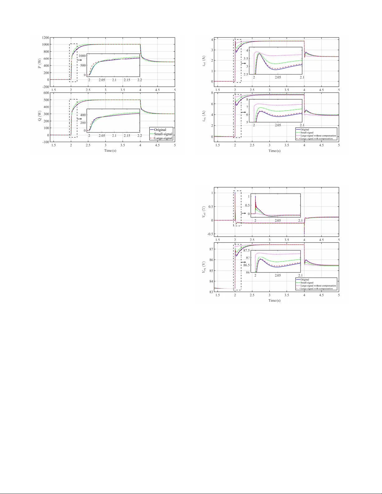
SUBMITTED TO IEEE FOR POSSIBLE PUBLICA TION. COPYRIGHT MA Y BE TRANSFERRED WITHOUT NOTICE 1 Singular Perturbation-based Lar ge-Signal Order Reduction of Microgrids for Stability and Accurac y Synthesis with Control Zixiao Ma, Member , IEEE, Zhaoyu W ang, Senior Member , IEEE, Y uxuan Y uan, Member , IEEE, T ianqi Hong, Member , IEEE, Abstract —With the increasing penetration of distrib uted en- ergy resour ces (DERs), it is of vital importance to study the dynamic stability of microgrids (MGs) with exter nal control inputs in the electromagnetic transient (EMT) time scale. This requir es detailed models of the underlying contr ol structure of MGs and results in a high-order nonlinear MG contr ol system. Higher -level controller design and stability analysis of such high- order systems ar e usually intractable and computation-costly . T o over come these challenges, this paper proposes a large-signal order reduction (LSOR) method for MGs with considerations of external control inputs and the detailed dynamics of underlying control levels based on singular perturbation theory (SPT). Specially , we innovativ ely proposed and strictly proved a general stability and accuracy assessment theorem that allo ws us to analyze the dynamic stability of a full-order nonlinear system by only le veraging its corresponding reduced-order model (ROM) and boundary layer model (BLM). Moreover , this theorem also theoretically provides a set of conditions under which the devel- oped R OM is accurate. Finally , by embedding such a theorem into the SPT , we propose a novel LSOR approach with guaranteed accuracy and stability analysis equiv alence. The pr oposed LSOR method is generic and can be applied to arbitrary dynamic systems. Multiple case studies are conducted on MG systems to show the effectiveness of the proposed approach. Index T erms —Microgrids, large-signal, order reduction, sin- gular perturbation, stability and accuracy assessment I . I N T RO D U C T I O N M ICR OGRIDS (MGs) are localized small-scale power systems composed of interconnected loads and dis- tributed energy resources (DERs) in low-v oltage and medium- voltage distribution networks. It can be operated in grid- connected and islanded modes [1]–[4]. The high penetration of lo w-inertia DERs makes the dynamic response of MGs dif- ferent from con ventional networks dominated by synchronous machines. This lo w-inertia characteristic highlights the im- portance of dynamic modeling, stability analysis, and control studies of MGs in the electromagnetic transient (EMT) time scale [5]–[7]. T o precisely capture the comprehensiv e transient dynamics of MGs in a hierarchical control structure, detailed dynamic models of the lower control levels such as primary and zero-control lev els, and the impact of external input from higher control lev els such as secondary control, need to be Z. Ma, Z. W ang and Y . Y uan are with the Department of Electrical and Computer Engineering, Iowa State Uni versity , Ames, IA, 50011 USA (E-mail: zma@iastate.edu; wzy@iastate.edu; yuanyx@iastate.edu). (Corresponding au- thor: Zhaoyu W ang.) T . Hong is with Energy System Di vision, Argonne National Laboratory , Lemont, IL. (Email: thong@anl.gov). taken into account. Ho wev er, the high-order nature of these detailed dynamics of the underlying control structures makes it intractable to analyze the stability of MGs with such a complex dynamic model [8]–[11]. In addition, another critical challenge brought by considering the underlying controllers is the two-time-scale behavior of MGs due to the dif ferent ev olutionary v elocities of different state variables, which leads to a stiff dif ferential equation problem [12]. In the dynamic simulation of MGs, numerically solving this stiff problem requires extremely small time steps, which results in an unmanageable computational complexity [13]. T o solve the above problems, model order reduction tech- niques hav e been studied and applied to power system anal- yses. In [14], [15], an aggregate equiv alent model was de- veloped for the order reduction of MGs by assuming similar in verter dynamics. Kron reduction was adopted to simplify the network of MGs in [16]. In [17], the authors used a balanced truncation method for DC MGs described by a linear model with inhomogeneous initial conditions. Although these methods can ef fectiv ely simplify the MG model, the time-scale separation problem aroused by the consideration of underlying control le vels for EMT analysis is still not solved. Giv en the inherent two-time-scale property of MGs, singular perturbation theory (SPT) is a suitable technology for this purpose. The SPT is a mathematical frame work that focuses on analyzing problems with a parameter , where the solutions of the problem at a specific limiting value of the parameter exhibit distinct characteristics compared to the solutions of the general problem, resulting in a singular limit. It facilitates the separation of the system into a reduced-order model (ROM) that captures the slow states, and a boundary layer model (BLM) that represents the errors between fast and quasi- steady states. It is worth noting that the terms “slow” and “fast” refer to the transient ev olutionary velocity of states in this context. Unlike con v entional model reduction methods that simply neglect certain state variables, SPT preserves the characteristics of fast dynamics by integrating them into the “slow” states, as advocated by [18]. Additionally , SPT has the advantage of con verting the original stiff problem into a non- stiff problem, resulting in improv ed computational efficiency . A spatiotemporal model reduction method of MGs using SPT and Kron reduction was proposed in [19], nonetheless, the method is not generic enough. In [20], [21], a linear SPT was applied to small-signal models of MGs. Howe ver , since it used the small-signal model, the result only holds in the SUBMITTED TO IEEE FOR POSSIBLE PUBLICA TION. COPYRIGHT MA Y BE TRANSFERRED WITHOUT NOTICE 2 neighborhood of a stable equilibrium point. The above studies focus on the dev elopment of the reduced- order MG modeling, whereas the stability assessment based on the deri ved R OM is not included. T o fill this gap, the system order is reduced for simplifying the stability analysis by neglecting the underlying voltage controller in [22] at the expense of losing fast dynamics. In [23], the nonlinear L yapuno v stability of DC/A C in v erters with different R OMs was studied. A method for simplifying the stability assessment was dev eloped and applied to an islanded MG with droop control by using inv erter angles in [24]. Nevertheless, it was demonstrated that such a simplification process could affect the accuracy of reduced models in [25], [26]. Moreov er, to our best knowledge, the existing studies do not consider the impact of e xternal inputs such as power commands and v oltage frequency references on MG stability analysis. A typical way is to consider the unforced system by neglecting the inputs to study the internal stability . Howe ver , e ven though the unforced system is stable, a continuous input signal can render the system unstable. In [27], a stability assessment criterion that used the input-to-state stability (ISS) of ROM and global asymptotic stability (GAS) of BLM was proposed to analyze the total stability of the original system. This method is generic for arbitrary singular perturbed systems under certain conditions, nev ertheless, the conv ergence of the error between reduced and original models is not theoretically analyzed, which hinders the accuracy ev aluation of reduced models. T o ov ercome the abov e challenges, this paper proposes a nov el large-signal order reduction (LSOR) strategy for in verter -based MGs with detailed dynamics of the underlying control le vels in the EMT time scale. Firstly , a general theorem for analyzing the dynamic stability of the full-order model by only alternatively assessing the stability of its deri ved R OM and BLM is proposed. A ke y point is that we consider ISS to quantify the system’ s response to external inputs and unify internal and e xternal stability . In particular, by assuming the R OM to be ISS, the unforced ROM to be e xponentially stable, and BLM to be uniformly GAS, one can prov e that the original system is totally ISS. Then, we dev elop the conditions that guarantee the accuracy of reduced models for both slow and fast dynamics. Finally , by embedding the proposed stability and accuracy assessment theorem into the large-signal SPT , an improv ed LSOR algorithm is proposed for MGs. Strict mathematical proof is provided to illustrate that the proposed order reduction technique is generic for arbitrary dynamic systems. The main contributions can be summarized as follo ws: • W e propose a general theorem that allo ws us to assess the large-signal stability of MGs with detailed dynamics of underlying controllers in the EMT time scale by only analyzing their R OMs and BLMs. • A set of accuracy criteria is developed, under which the error between the reduced and original models is bounded and con ver ges as the perturbation coefficients decrease. • The impact of external control input from the higher control le vel on the above stability and accuracy analyses is studied with strict mathematical proof. • The stability and accuracy assessment synthesis is em- bedded into the LSOR method to improve the model accuracy via a feedback mechanism, which automatically tunes the bounds of perturbation coefficients as an index for identifying the slo w and fast dynamics. The rest of the paper is org anized as follows. Section II describes the lar ge-signal mathematical model of the stud- ied MG system. Section III introduces the general singular perturbation theory and proposes our stability and accuracy assessment theory . Section IV gives the simulation validation of the proposed method. Section V concludes the paper . I I . L A R G E - S I G N AL M O D E L I N G O F I N V E RT E R - B A S E D M G S This section introduces a nonlinear model of the studied MG system with detailed primary and zero-control le vels. Depending on the research objectiv es, control strategies, and operation modes, MGs may hav e different models. According to [20], the transient response velocity of line dynamics is much faster than the slow ones in DERs due to the small line impedance. Moreover , the state equations are fully decoupled between DERs and lines. As a result, the line dynamics can be neglected. Therefore, this section focuses on the modeling of DERs, which are the main dynamic components in an in verter- based MG. A general control diagram of DERs is sho wn in Fig. 1. The model can switch between two subsystems according to the MG operation modes. In grid-tied mode, OM flag switches to 1 , then the voltage source in verter (VSI) is controlled by the power controller and current controller to follow the power command P ∗ , Q ∗ . The MG bus voltage and system frequency are maintained by the main grid. In islanded mode, OM flag is set to 0 , and the MG voltage and frequency are regulated by the DERs using droop controllers. According to Fig. 1, the mathematical model can be derived for each component where i = 1 , . . . , N denotes the index of N DERs in the MG. A. A vera ge P ower Calculation The generated activ e and reactive power can be calculated using the transformed output voltage v odq and current i odq . Using a low-pass filter (LPF) with the corner frequenc y ω c , we can obtain the filtered instantaneous powers as follo ws, ˙ P i = − P i ω c i + 1 . 5 ω c i ( V od i I od i + V oq i I oq i ) , (1a) ˙ Q i = − Q i ω c i + 1 . 5 ω c i ( V oq i I od i − V od i I oq i ) . (1b) B. Phase Lock Loop The model of phase lock loop (PLL) is the same as that established in [20] as follo ws, ˙ V odf i = ω cPLL i V od i − ω cPLL i V odf i , (2a) ˙ Φ PLL i = − V odf i . (2b) In grid-tied mode, the in verter output phase is synchronized to the main grid using PLL, therefore the deri vati ve of phase angle δ i is set to ω PLL i : ˙ δ i = ω PLL i = 377 − K P , PLL i V odf i + K I , PLL i Φ PLL i . (3) In islanded mode, the phase angle of the first in verter can be arbitrarily set as the reference for the other inv erters: ˙ δ i = ω PLL1 − ω PLL i . (4) SUBMITTED TO IEEE FOR POSSIBLE PUBLICA TION. COPYRIGHT MA Y BE TRANSFERRED WITHOUT NOTICE 3 V dc i V S I L P F D r o o p C o n t r o l l e r V o l t a g e C o n t r o l l e r C u r r e n t C o n t r o l l e r S V P WM dq a b c P o w e r C o n t r o l l e r P L L P o w e r c a l c u l a t o r dq a b c dq a b c L P F 𝑃 𝑖 , 𝑄 𝑖 𝑉 𝑜 𝑞 𝑖 ∗ , 𝜔 𝑖 ∗ 𝑃 𝑖 ∗ , 𝑄 𝑖 ∗ 𝑉 𝑜 𝑞 𝑖 𝜔 𝑃 𝐿 𝐿 𝑖 1 0 𝑂 𝑀 𝑓 𝑙 𝑎 𝑔 𝐼 𝑑 𝑞 𝑖 ∗ 𝐼 𝑑 𝑞 𝑖 𝛿 𝑖 𝑉 𝑙 𝑑 𝑞 𝑖 ∗ 𝑉 𝑙 , 𝑎 𝑏 𝑐 𝑖 ∗ 𝑠 𝑤 𝑃 𝑖 , 𝑄 𝑖 𝑝 𝑖 , 𝑞 𝑖 𝐼 𝑜 𝑑 𝑞 𝑖 𝑉 𝑜 𝑑 𝑞 𝑖 𝐼 𝑙 , 𝑎 𝑏 𝑐 𝑖 𝛿 𝐿 𝑓 𝑖 𝑅 𝑓 𝑖 𝑉 𝑜 , 𝑎 𝑏 𝑐 𝑖 𝐿 𝑐 𝑖 𝑅 𝑐 𝑖 𝑉 𝑏 , 𝑎 𝑏 𝑐 𝑖 𝐵 𝑢 𝑠 𝑖 𝐶 𝑓 𝑖 𝑅 𝑑 𝑖 𝑉 𝑜 , 𝑎 𝑏 𝑐 𝑖 𝐼 𝑜 , 𝑎 𝑏 𝑐 𝑖 Fig. 1. The diagram of VSI-based DER and controller block. C. P ower Contr ollers In grid-tied mode, the output power of DER is regulated by the power controller using the PI control method. The input references are the commanded real and reactive powers: ˙ Φ P i = P i − P ∗ i , (5a) I ∗ lq i = K I , P i Φ P i + K P , P i ˙ Φ P i , (5b) ˙ Φ Q i = Q i − Q ∗ i , (5c) I ∗ ld i = K I , P i Φ Q i + K P , P i ˙ Φ Q i . (5d) D. V oltage Controller s and Dr oop Contr ollers In islanded mode, a DER has no reference inputs from the main grid. Therefore, it must generate its only voltage and frequency references using droop controllers as follows, ω ∗ i = ω n i − m i P i , (6a) V ∗ oq i = V oq , n i − n i Q i . (6b) These references will be used as the set points for voltage controllers. T wo PI controllers are adopted for the voltage controllers as follo ws, ˙ Φ d i = ω PLL i − ω ∗ i , (7a) I ∗ ld i = K I , V i Φ d i + K P , V i ˙ Φ d i , (7b) ˙ Φ Q i = V ∗ oq i − V oq i , (7c) I ∗ lq i = K I , V i Φ q i + K P , V i ˙ Φ q i . (7d) E. Curr ent Contr ollers The PI controllers are adopted for current controllers. They generate the commanded voltage reference V ∗ ldq i according to the error between the inductor currents reference I ∗ ldq i and its feedback measurements I ldq i : ˙ Γ d i = I ∗ ld i − I ld i , (8a) V ∗ ld i = − ω n i L f i I lq i + K I , C i Γ d i + K P , C i ˙ Γ d i , (8b) ˙ Γ q i = I ∗ lq i − I lq i , (8c) V ∗ lq i = − ω n i L f i I ld i + K I , C i Γ q i + K P , C i ˙ Γ q i . (8d) F . LC F ilters and Coupling Inductors The dynamical models of LC filters and coupling inductors are as follo ws, ˙ I ld i = ( − R f i I ld i + V ld i − V od i ) /L f i + ω n i I lq i , (9a) ˙ I lq i = ( − R f i I lq i + V lq i − V oq i ) /L f i − ω n i I ld i , (9b) ˙ I od i = ( − R c i I od i + V od i − V bd i ) /L c i + ω n i I oq i , (9c) ˙ I oq i = ( − R c i I oq i + V oq i − V bq i ) /L c i − ω n i I od i , (9d) ˙ V od i = ( I ld i − I od i ) /C f i + ω n i V oq i + R d i ( ˙ I ld i − ˙ I od i ) , (9e) ˙ V oq i = ( I lq i − I oq i ) /C f i − ω n i V od i + R d i ( ˙ I lq i − ˙ I oq i ) . (9f) In conclusion, when the MG system is operating in grid-tied mode, the mathematical model can be represented by equations (1)-(3), (5) and (8)-(9). In islanded mode, the MG model can be represented by equations (1)-(2), (4) and (6)-(9). I I I . I M P RO V E D L S O R B Y E M B E D D I N G S T A B I L I T Y A N D A C C U R A C Y A S S E S S M E N T T H E O R E M In this section, we propose an impro ved LSOR method together with stability and accuracy assessment synthesis. Firstly , we briefly present the SPT -based LSOR approach. Then a nov el large-signal stability and accuracy assessment theorem with consideration of external control input is pro- posed. Finally , we impro ve the LSOR algorithm by embedding the stability and accuracy assessment theorem, so that it can guarantee the accuracy of deriv ed R OM and efficiently ev aluate the stability of original models. The proposed LSOR strategy is essentially generic and is suitable for the above MG model introduced in Section II. A. LSOR Appr oach using the SPT for MGs Due to the two-time-scale property , the dynamics of MGs can be classified as slow and fast dynamics according to the transient velocity . The main idea of SPT is to freeze the fast dynamics and degenerate them into static equations. Thus, the R OM can be obtained by substituting the solutions of the static equations into the slo w dynamic equations. SUBMITTED TO IEEE FOR POSSIBLE PUBLICA TION. COPYRIGHT MA Y BE TRANSFERRED WITHOUT NOTICE 4 Consider an MG system in the following general singular perturbed form, ˙ x ( t ) = f ( x ( t ) , z ( t ) , u ( t ) , ε ) , (10a) ε ˙ z ( t ) = g ( x ( t ) , z ( t ) , u ( t ) , ε ) , (10b) where x ∈ R n , z ∈ R m represent the fast and slow state variables of MGs, respectively , such as voltages and currents; u ∈ R p denotes the continuous MG inputs such as power commands, or voltage frequency commands. ε denotes the small parameters in MGs such as capacitances and inductances named as perturbation coef ficient. f and g are locally Lipschitz functions on their ar guments. For simplicity , we neglect the notation of time-dependency ( t ) in the rest of this paper . Since ε is small, the fast transient velocity ˙ z = g /ε can be much larger than the slo w dynamics ˙ x . T o solve this two- time-scale problem, we can set ε = 0 , then equation (10b) degenerates to the following algebraic equation, 0 = g ( x , z , u , 0) . (11) If equation (11) has at least one isolated real root and satisfies the implicit function theory , then for each argument, we hav e the following closed-form solution, z = h ( x , u ) . (12) Substitute equation (12) into equation (10a) and let ε = 0 , we hav e a quasi-steady-state (QSS) model, ˙ x = f ( x , h ( x , u ) , u , 0) . (13) Note that the order of the QSS system (13) drops from n + m to n . The inherent two-time-scale property can be described by introducing the BLM. Define a fast time scale variable τ = t/ε , and a new coordinate y = z − h ( x , u ) . In this ne w coordinate, equation (10b) is re written as d y dτ = g ( x , y + h ( x , u ) , u , ε ) − ε  ∂ h ∂ x f ( x , y + h ( x , u ) , u , ε ) + ∂ h ∂ u ˙ u  . (14) Let ε = 0 , we obtain the BLM as follows, d y dτ = g ( x , y + h ( x , u ) , u , 0) . (15) B. Stability and Accuracy Assessment Theorem In this subsection, we propose a criterion to assess the stability of the original system and the accuracy of R OM and BLM. Considering the impact of e xternal inputs on the stability of MGs, we define the ISS as follows. Definition 1 (ISS): Consider such a nonlinear system ˙ x = ˜ f ( x , v 1 , v 2 ) (16) where x ∈ R n is the state vector , v 1 ∈ R m , v 2 ∈ R p are input vectors, and ˜ f is locally Lipschitz on R n × R m × R p . The system (16) is ISS with L yapuno v gains α v 1 and α v 2 of class kappa ( K ), if there exists a class kappa-ell ( KL ) function β such that for x (0) ∈ R n and bounded inputs v 1 , v 2 , the solution of (16) exists and satisfies k x ( t ) k 6 β ( k x (0) k , t ) + α v 1 ( k v 1 k ) + α v 2 ( k v 2 k ) . (17) The above definition indicates that an MG system is ISS when all the trajectories are bounded by some functions of the input magnitudes. Then we giv e the following three as- sumptions which are the sufficient conditions for the theorem. Assumption 1 (Gr owth conditions): The functions f , g , and their first partial deriv ativ es are continuous and bounded with respect to ( x , z , u , ε ) ; h and its first partial deriv ati ves ∂ h /∂ x , ∂ h /∂ u is locally Lipschitz; and the Jacobian ∂ g /∂ z has bounded first partial deriv ativ es with respect to its arguments. Assumption 2 (Stability of R OM): The R OM (13) is ISS with L yapunov gain ˆ α x , and its unforced system has an exponentially stable equilibrium at the origin. Assumption 3 (Stability of BLM): The origin of the BLM (15) is a GAS equilibrium, uniformly in x ∈ R n , u ∈ R p . Remark 1: The conditions in Assumption 1 are commonly satisfied for most MGs [25]. Inspired by [27], we propose the stability and accuracy assessment of MGs as the following theorem. Note that the conditions, results and proof of our theorem and [27] are dif ferent. In [27], only the stability of the original system is proved, nonetheless, the accuracy of the ROM and BLM is not analyzed, which is of vital importance to make sure that the deriv ed reduced-order model is correct. Howe ver , the addition of accuracy analysis arouses new challenges in the proof which cannot be solved by directly using [27]. Therefore, we add a constraint condition on the transient speed in Assumption 2 and propose a new proving method for our theorem. Theor em 1: If the MGs system (10), its ROM (13) and the BLM (15) satisfy the Assumptions 1-3, then for each pair of ( µ, ξ ) , there exists a positiv e constant ε ∗ , such that for all t ∈ [0 , ∞ ) , max {k x (0) k , k y (0) k , k u k , k ˙ u k} 6 µ , and ε ∈ (0 , ε ∗ ] the errors between the solutions of the original MGs system (10) and its ROM (13) and BLM (15) satisfy k x ( t, ε ) − ˆ x ( t ) k = O ( ε ) , (18) k z ( t, ε ) − h ( ˆ x ( t ) , u ( t )) − ˆ y ( t/ε ) k = O ( ε ) , (19) where ˆ x ( t ) and ˆ y ( τ ) are the solutions of R OM (13) and BLM (15), respecti vely . k x − ˆ x k = O ( ε ) means that k x − ˆ x k 6 k k ε k for some positi ve constant k. Furthermore, for any giv en T > 0 , there exists a positive constant ε ∗∗ 6 ε ∗ such that for t ∈ [ T , ∞ ) and ε < ε ∗∗ , it follo ws uniformly that k z ( t, ε ) − h ( ˆ x ( t ) , u ( t )) k = O ( ε ) . (20) Moreov er , there exist class K L functions β x , β y , a L ya- punov gain α x of class K and positiv e constants ξ , such that the solutions of the original MGs system (10a) and (14) exist and satisfy k x ( t, ε ) k 6 β x ( k x (0) k , t ) + α x ( k u k ) + ξ , (21) k y ( t, ε ) k 6 β y  k y (0) k , t ε  + ξ . (22) Remark 2: Theorem 1 indicates large-signal stability by observing that µ can be arbitrarily large. This is more com- prehensiv e than the small-signal stability studied in [20]. Moreov er , the errors between the solutions of reduced and original MGs should be small and bounded to guarantee accuracy . (18) and (19) show that for suf ficiently small ε , SUBMITTED TO IEEE FOR POSSIBLE PUBLICA TION. COPYRIGHT MA Y BE TRANSFERRED WITHOUT NOTICE 5 these errors tend to be zero. Equation (20) means that for small enough ε , the solution ˆ y of the BLM decays to zero exponentially fast in time T , so that the fast solutions can be estimated by only QSS solutions h ( t, ¯ x ( t )) after time T . Remark 3: According to the theorem, if the R OM is ISS and BLM is GAS, then the original system is stable as shown in (21) and (22). Moreo ver , in real physical systems, one challenge of SPT is how to identify the slow and fast dynamic states. A commonly-used approach is the knowledge discov er-based method that relies on expert knowledge for specific domains. For example, in MGs, some small parasitic parameters such as capacitances, inductances, and small time constants, can be selected as the perturbation coefficients ε . The states with respect to these small ε are identified as fast states. This conv entional empirical identification method falls short of ef ficiency and accuracy . Therefore, we propose a more ef ficient and accurate method to identify the slo w/fast dynamics by finding the bound of ε in the following proof. Pr oof: Firstly , the stability of y (22) has already been prov ed by [27] using the conv erse theorem, causality , signal truncation, and Assumption 3. Then, we directly use its result to prove the accuracy of the reduced model (18)-(20). Define the error between solutions of reduced and original slow dynamics as E x = x − ˆ x . When ε = 0 , y = z − h ( x , u ) = 0 . Then, we hav e ˙ E x = f ( E x , 0 , u , 0) + ∆ f , (23) where ∆ f = [ f ( ˆ x + E x , 0 , u , 0) − f ( ˆ x , 0 , u , 0) − f ( E x , 0 , u , 0)] + f ( x , y , u , ε ) − f ( x , 0 , u , 0) . According to Assumption 1, it follows that k ∆ f k 6 ` 1 k E x k 2 + ` 2 k E x k k ˆ x k + ` 3 β y  k y (0) k , t ε  + ` 3 ξ + ` 4 ε, (24) for some positi ve constants ` 1 , ` 2 , ` 3 , ` 4 . The last term in system (23) can be vie wed as a perturbation of ˙ E x = f ( E x , 0 , u , 0) . (25) Since the origin of the system (25) is exponentially stable with u = 0 , using the con verse theorem, there exist a L ya- punov function V 2 ( E x ) , and positive constants c 1 , c 2 , c 3 , c 4 , for which it follo ws that c 1 k E x k 2 6 V 2 ( E x ) 6 c 2 k E x k 2 , (26) ∂ V 2 ∂ E x f ( E x , 0 , u , 0) 6 − c 3 k E x k 2 , (27)     ∂ V 2 ∂ E x     6 c 4 k E x k . (28) Using (22), (24) and (26)-(28), the L yapunov function of (25) along the trajectory of (23) satisfies ˙ V 2 = ∂ V 2 ∂ E x f ( E x , 0 , u , 0) + ∂ V 2 ∂ E x ∆ f 6 − c 3 k E x k 2 + c 4 k E x k h ` 1 k E x k 2 + ` 2 k E x k k ˆ x k + ` 3 β y  k y (0) k , t ε  + ` 3 ξ + ` 4 ε  . (29) For k E x k 6 c 3 / (2 c 4 ` 1 ) , using Assumption 2, it follows that ˙ V 2 6 − 2 n c 3 − c 4 ` 1 h ˆ β x ( k ˆ x (0) k , t ) + ˆ α x ( k u k ) io V 2 + 2  ` 3 ε + ` 3 ξ + ` 4 β y  k y (0) k , t ε  p V 2 6 − 2 n ` a − ` b ˆ β x ( k ˆ x (0) k , t ) o V 2 + 2  ` c ε + ` d β y  k y (0) k , t ε  p V 2 , (30) where 0 < ` a 6 c 3 − c 4 ` 1 ˆ α x ( sup k u k ) , ` c > ` 3 (1 + ξ /ε ) > 0 , and ` b , ` d > 0 . Using the comparison lemma, we hav e W 2 ( t ) 6 φ ( t, 0) W 2 (0) + Z t 0 φ ( t, s )  ` c ε + ` d β y  k y (0) k , t ε  ds, (31) where W 2 = √ V 2 and | φ ( t, s ) | 6 ` e e − ` f t , f or ` e , ` f > 0 . (32) Because Z t 0 e − ` f t β y  k y (0) k , t ε  ds = O ( ε ) , (33) it can be verified that W 2 ( t ) = O ( ε ) . Then it follows that E x ( t, ε ) = O ( ε ) , and this means that (18) holds. Since we hav e already verified that (22) holds in the first step, then by Assumption 3, it follows that E y ( t, ε ) = k z ( t, ε ) − h ( ˆ x ( t, ε ) , u ( t )) − ˆ y ( t/ε ) k = k y ( t, ε ) − ˆ y ( t/ε ) k 6 k y ( t, ε ) k + k ˆ y ( t/ε ) k (34) 6 β y ( k y (0) k , t/ε ) + α y ( ε ) + ˆ β y ( k ˆ y (0) k , t/ε ) = O ( ε ) for given initial points and all t > 0 . This proves (19). According to Assumption 3, ˆ y ( t/ε ) = ˆ β y ( k y (0) k , t/ε ) → 0 as ε → 0 . Thus, the term ˆ y ( t/ε ) = O ( ε ) for all t > T > 0 if ε is small enough to satisfy ˆ β y ( k y (0) k , t/ε ) 6 k ε (35) Let ε ∗∗ and T denote a solution of (35) with equal sign. Subsequently , (20) holds for all ε 6 ε ∗∗ uniformly on [ T , ∞ ) . Finally , we prov e the ISS of original slow dynamics. Since k x ( t, ε ) k − k ˆ x ( t ) k 6 k x ( t, ε ) − ˆ x ( t ) k = O ( ε ) , (36) there exist some class KL function β x , class K function α and a small positi ve constant ε 3 , such that the solution of (10a) exists for all t > 0 and ε 6 ε ∗ := min { ε 1 , ε 2 , ε 3 } satisfying k x ( t, ε ) k 6 k ˆ x ( t ) k + O ( ε ) 6 ˆ β x ( k ˆ x (0) k , t ) + ˆ α x ( k u k ) + O ( ε ) 6 β x ( k x (0) k , t ) + α x ( k u k ) + ξ . (37) This completes the proof of (21). C. Stability and Accuracy Assessment Embedded LSOR This subsection dev elops a novel LSOR method by embed- ding the abo ve theorem. The ov erall flowchart is sho wn in Fig. 2 and the detailed algorithm is proposed in Alogrithm 1 . This algorithm is designed for MGs with two-time-scale properties, howe ver , no basic assumptions of the MGs are required. Therefore, the proposed method can be applied to arbitrary dynamic systems. SUBMITTED TO IEEE FOR POSSIBLE PUBLICA TION. COPYRIGHT MA Y BE TRANSFERRED WITHOUT NOTICE 6 O r i gi n al S ys t e m S t a b i l i t y A s s e s s m e n t A c c u r a c y A s s e s s m e n t 𝑥 𝑦 𝜀 ∗ 𝜀 ∗ ∗ T r a de - of f be t w e e n A c c ur a c y a nd E f f i c i e nc y T h e R O M an d B L M ar e ac c u r at e an d O r i gi n al S ys t e m i s s t ab l e G A S of B L M I S S of R O M S l ow / F a s t D yna m i c s I de nt i f i c a t i on R O M / B L M C a ndi da t e s 𝑥 𝑧 U n s t ab l e S t a bl e ε > 𝜀 ∗ D e t e r m i ni ng t he B ou nd o f P e r t ur ba t i on C oe f f i c i e nt s Fig. 2. The diagram of stability and accuracy assessment embedded LSOR. 37 34 12 5 2 1 13 4 14 15 18 17 7 16 6 19 22 35 20 21 3 23 9 24 36 25 8 29 10 28 26 27 30 31 11 32 33 P C C Bus w i t h i nve rt e r Bu s w i t hou t i nve rt e r Fig. 3. The diagram of modified IEEE-37 bus system. I V . C A S E S T U D Y A. Simulation Setup The proposed method is tested on a modified IEEE-37 bus MG, which can be operated in grid-tied or islanded modes as shown in Fig. 3. According to [19], se ven inv erters are connected to buses 15, 18, 22, 24, 29, 33, and 34. When PCC is closed, the MG is operated in grid-tied mode. Otherwise, it is operated in islanded mode. W e first let the MG be operated in grid-tied mode. In order to analyze the detailed dynamic properties of both slo w and fast dynamics as well as compare our method with the small- signal order reduction approach, a single bus of interest (bus 34) is chosen to show its dynamic responses after po wer command (input) changes for clearance. Then, a simulation is conducted in islanded mode to show the dynamic responses of multiple b uses with DERs when a large load sudden change is gi ven to verify its ef fectiveness against large disturbances. The detailed load and line parameter settings can be found in [19]. B. P erformance in Grid-tied Mode and Comparison W ith Small-Signal R OM According to the Algorithm 1 in section III-C, we first iden- tify the slo w and fast dynamics by finding the ε . Considering the MG model in grid-tied mode, the deriv ativ e term can be Algorithm 1 Stability/Accuracy Assessment Embedded LSOR 1: Choose the smaller parameters dominating the transient velocity as ε . The states with respect to ε are identified as fast states, while the others as slow states. 2: procedur e RO M A N D B L M D E R I V A T I O N 3: Let ε = 0 , solve the algebraic equation (11) to obtain the isolated QSS solutions z = h ( x , u ) 4: Substitute z into (10a), obtaining the ROM (13) 5: Deriv e the BLM using equation (15). 6: end procedur e 7: procedur e S TA BI L I T Y A S S E S S M E N T 8: if Assumption 2 and 3 ar e satisfied then 9: Go to next procedure 10: else 11: Return to Step 1 to re-identify slow/f ast dynamics. 12: end if 13: end procedur e 14: procedur e C A L C U L A T E T H E B O U N D O F ε 15: Calculate ε ∗ = min { ε 1 , ε 2 , ε 3 } according to proof. 16: Calculate ε ∗∗ by solving equation (35) with equal sign. 17: end procedur e 18: procedur e A C C U R A C Y A S S E S S M E N T 19: if ε 6 ε ∗ then 20: if ε 6 ε ∗∗ then 21: z = h ( ˆ x , u ) is the solution of fast dynamics 22: else 23: Use z = h ( ˆ x , u ) + ˆ y by solving the BLM (15). 24: end if 25: else 26: Return to Step 1 to re-identify slo w/fast dynamics 27: end if 28: end procedur e rewritten as  1 ω c ˙ P i , 1 ω c ˙ Q i , ˙ Φ PLL i , ˙ δ i , K P , P i K I , P i ˙ Φ P i , K P , P i K I , P i ˙ Φ Q i , K P , C i K I , C i ˙ Γ d i , K P , C i K I , C i ˙ Γ q i , 1 ω c , PLL i ˙ V od , f i , L f i ˙ I ld i , L f i ˙ I lq i , L c i ˙ I od i , L c i ˙ I oq i , C f i ˙ V od i , C f i ˙ V oq i i T (38) Substituting the parameters in [19] into the vector (38), it can be seen that the magnitudes of dif ferent parameters vary significantly , which is caused by the two-time-scale property of the system. The smaller parameters are selected as perturbation coefficients ε , which are utilized to classify the slow and fast states in this system: x 1 = [ P i , Q i , Φ PLL i , δ i , Φ P i , Φ Q i , Γ d i , Γ q i , ] T , (39) z 1 = [ V odf i , I ld i , I lq i , I od i , I oq i , V od i , V oq i ] T . (40) W e first set ε to 0 and calculate the QSS solution z 1 = h ( x 1 , u 1 ) by solving the algebraic equation with respect to the fast dynamics (40). Then the R OM is obtained by substituting z 1 into the slo w dynamic equations with respect to (39). Comparing the numbers of state variables in equation (38) and (39), the order of the original model is reduced to 53 . 33% . SUBMITTED TO IEEE FOR POSSIBLE PUBLICA TION. COPYRIGHT MA Y BE TRANSFERRED WITHOUT NOTICE 7 Fig. 4. Simulation results of slo w and f ast dynamic responses of interested bus: active and reactive power . Then we derive the BLM using equation (15). Once the ROM and BLM are obtained, we use the con ventional ISS and GAS judging theorems in [18] to ev aluate their stability of them. Specially , the unforced nonlinear R OM is exponentially stable by checking that its linearized system matrix has eigenv alues with strictly negati ve real parts. It can be verified that the assumptions are satisfied. Based on this result, we are inclined to anticipate the stability of the original system. T o ensure this, we still need to theoretically verify the accuracy of the ROM and BLM. F ollowing the technique in the proof, we can calculate the boundary of ε as ε ∗ = min { ε 1 , ε 2 , ε 3 } = 7 . 92 × 10 − 3 . Note that max { ε } = 3 . 9 × 10 − 3 < 7 . 92 × 10 − 3 = ε ∗ . Therefore, we can conclude that this MGs system is stable and we can use the solutions of its R OM ˆ x and z = h ( ˆ x , u ) + ˆ y to accurately represent its real dynamic responses. Furthermore, giv en T = 0 . 43 s, we can find a ε ∗∗ satisfying max { ε } < ε ∗∗ = 4 . 2 × 10 − 3 , which indicates that the term ˆ y will be O ( ε ) after 0 . 43 s. Here, a trade-off e xists between accurac y and efficiency . When the accuracy is prior, one can choose z = h ( ˆ x , u ) + ˆ y by computing an additional differential equation (BLM). When the efficienc y dominates, use z = h ( ˆ x , u ) suffering the inaccuracy only within (0 , T ) . Then we conduct the simulation of the derived R OM using Matlab . The activ e power command changes to 1000 W at 2 s and changes to 500 W at 4 s. The reactiv e power command changes to 500 W at 2 s and changes to 300 W at 4 s. A comparison simulation using the small-signal order reduction method in [20] is conducted under the same conditions. The simulation results are sho wn in Fig. 4-6, where blue solid lines denote the responses of the original model, green dash-dotted lines denote that using small-signal order reduction method, pink dotted lines denote the results of proposed LSOR without BLM compensation (i.e., QSS solution), and red dashed lines are the responses with the addition of solution ˆ y of BLM (i.e. z = h + ˆ y ). For the main slow dynamics (acti ve and reactiv e powers) shown in (a), the proposed LSOR method is Fig. 5. Simulation results of slo w and f ast dynamic responses of interested bus: dq -axis output currents i od and i oq Fig. 6. Simulation results of slo w and f ast dynamic responses of interested bus: dq -axis output voltages V od and V oq . more accurate than the small-signal model during the transient period. As for the main fast dynamics v oltages and currents shown in (b) and (c), the result of LSOR with compensation ˆ y giv es the most precise performance. Ho wev er , the LSOR without ˆ y giv es worse performance than the small-signal one used in [20]. This is because the fast dynamics predicted by the method in [20] are also compensated with a corrected response. From the stability point of view , the red lines in Fig. 4-6 show that, with bounded input po wer commands, both R OM and BLM are stable, which indicates that the original system is stable as justified by the stability of blue lines. In order to ev aluate the computational performance, two different ordinary differential equation (ODE) solvers are adopted: ode45 solver and ode15s solver . The ode45 solver uses the 4th-order Runge-K utta method with variable step sizes in order to solve the non-stiff ODE problems, whereas the ode15s solver is designed for stiff problems. The computa- SUBMITTED TO IEEE FOR POSSIBLE PUBLICA TION. COPYRIGHT MA Y BE TRANSFERRED WITHOUT NOTICE 8 T ABLE I C O MP U TA T IO N AL T I M E O F O RI G I NA L A ND R E D UC E D - OR D E R M O D E LS U S IN G D I FFE R E N T O D E S O L V E R S I N G R ID - T I ED M O D E . Solver Model Original model Reduced model Percentage ode45 94 . 25 s 11 . 92 s 87 . 4% ode15s 11 . 43 s 10 . 81 s 5% tional time is shown in T able I. This comparison indicates that our LSOR method conv erts the original model from a stiff ODE problem to a non-stiff one. The adoption of the proposed method also improves the stability of the ODE-solving process through this conv ersion. In conclusion, the proposed method can reduce the computational time from tw o aspects: the order of the system and the stiffness of the ODE problem. Remark 4: Note that with the addition of the solution of BLM, we need to solve another set of differential equations. This seems that the proposed method has limited ability to reduce the computational b urden. Ho wever , this is not the case. As discussed abov e, SPT reduces the computational burden not only by reducing the number of dif ferential equations but also by con verting the stiff problem to a non-stiff one. Moreov er , the adopted e xample is a possible worst case that the perturbation coefficients are not small enough. When ε is sufficiently small, the con v erging time T can be sufficiently small as well. Then we can directly use the algebraic equation to estimate the fast states. C. P erformance in Islanded Mode under Lar ge Disturbances In this subsection, a simulation in islanded mode is con- ducted to verify the effecti veness of the proposed method by showing the dynamic responses of the b uses with DERs. T o study the dynamic characteristics, a 20 Ω load is connected parallel to bus 12 at 2 s and disconnected at 2 . 5 s. Follo wing the similar procedure in case 1, we can identify the slo w and fast dynamics of this multi-bus system. Despite the different parameter settings of in verters, the relative magnitudes of deriv ati ve terms’ coefficients still hold uniformly . That means we can obtain a uniform division of slow and fast dynamics. This fact is based on the nature of different components’ time scales. The slo w and fast states are divided as follows, x 2 = [ P i , Q i , Φ PLL i , δ i , Φ d i , Φ q i , Γ d i , Γ q i , ] T , (41) z 2 = [ V odf i , I ld i , I lq i , I od i , I oq i , V od i , V oq i ] T . (42) The R OM can be derived using the Algorithm 1 . The order of the original model is reduced from 105 th to 56 th . The simulation time is sho wn in T able II. Same as analyzed in the last case study , the proposed method can con vert the stiff model of islanded MG to a non-stiff one to reduce the computational b urden. Fig. 7-9 show the dynamic responses of the original and reduced models of sev en buses with DERs. The comparison between the results of the original model and the reduced one shows the accuracy of the ROM. In addition, the responses under load sudden change verify Fig. 7. Comparison of the activ e/reactive power of the sev en buses with DERs of original and reduced systems: (a)-(b) denote the responses of the reduced-order system, (c)-(d) are the responses of the original system. Fig. 8. Comparison of the dq -axis output currents of the se ven buses with DERs of original and reduced systems: (a)-(b) denote the responses of the reduced-order system, (c)-(d) are the responses of the original system. the ef fectiveness of our method against large disturbances in islanded systems. T ABLE II C O MP U TA T IO N AL T I M E O F O RI G I NA L A ND R E D UC E D - OR D E R M O D E LS U S IN G D I FFE R E N T O D E S O L V E R S I N I S LA N D E D M O D E . Solver Model Original model Reduced model Percentage ode45 104 . 25 s 11 . 25 s 89 . 2% ode15s 13 . 23 s 11 . 37 s 14% V . C O N C L U S I O N This paper proposes a large-signal order reduction (LSOR) approach for MGs in the electromagnetic transient (EMT) time SUBMITTED TO IEEE FOR POSSIBLE PUBLICA TION. COPYRIGHT MA Y BE TRANSFERRED WITHOUT NOTICE 9 Fig. 9. Comparison of the dq -axis output v oltages of the sev en buses with DERs of original and reduced systems: (a)-(b) denote the responses of the reduced-order system, (c)-(d) are the responses of the original system. scale with consideration of e xternal control input by synthesiz- ing a novel stability and accurac y assessment theorem. The ad- vantages of our proposed theorem can be summarized into two aspects. Firstly , one can determine the stability of a full-order system by only analyzing the stability of its derived reduced- order model (R OM) and boundary layer model (BLM). Spe- cially , when the R OM is input-to-state stable and the BLM is uniformly globally asymptotically stable, the original MGs system can be prov ed to be stable under sev eral common growth conditions. This makes it easier and more feasible to determine the stability of a high-order system. Secondly , a set of quantitati ve accuracy assessment criteria is developed and embedded into a tailored feedback mechanism to guarantee the accuracy of the deriv ed ROM. It is proved that the errors between solutions of reduced and original models are bounded and con ver gent under such conditions. The abov e stability and accuracy theorem has been strictly proven indicating that the proposed method is generic for arbitrary dynamic systems satisfying the gi ven assumptions. Finally , we have conducted multiple simulations under different conditions on an IEEE standard MG system to verify the ef fecti veness of the proposed method. R E F E R E N C E S [1] M. Shahidehpour, “Role of smart microgrid in a perfect power system, ” in Pr oc. IEEE PES General Meeting , Jul. 2010, p. 1. [2] M. Shahidehpour and J. F . Clair, “ A functional microgrid for enhancing reliability , sustainability , and energy efficienc y , ” Electr . J. , vol. 25, no. 8, pp. 21 – 28, Oct. 2012. [3] Z. Ma, Z. W ang, Y . Guo, Y . Y uan, and H. Chen, “Nonlinear multiple models adaptive secondary v oltage control of microgrids, ” IEEE Tr ans. Smart Grid , vol. 12, no. 1, pp. 227–238, Jan. 2021. [4] Q. Zhang, Z. Ma, Y . Zhu, and Z. W ang, “ A two-level simulation- assisted sequential distribution system restoration model with frequency dynamics constraints, ” IEEE T rans. Smart Grid , vol. 12, no. 5, pp. 3835– 3846, Sept. 2021. [5] Z. W ang, B. Chen, J. W ang, J. Kim, and M. M. Begovic, “Robust optimization based optimal dg placement in microgrids, ” IEEE Tr ans. Smart Grid , vol. 5, no. 5, pp. 2173–2182, Sep. 2014. [6] X. Lu, K. Sun, J. M. Guerrero, J. C. V asquez, L. Huang, and J. W ang, “Stability enhancement based on virtual impedance for DC microgrids with constant power loads, ” IEEE T r ans. Smart Grid , vol. 6, no. 6, pp. 2770–2783, No v . 2015. [7] Z. Ma, Q. Zhang, and Z. W ang, “Safe and stable secondary voltage control of microgrids based on explicit neural networks, ” IEEE T rans. Smart Grid , 2023, early access. doi=10.1109/TSG.2023.3239548. [8] Y . Li, P . Zhang, L. Zhang, and B. W ang, “ Acti ve synchronous detection of deception attacks in microgrid control systems, ” IEEE Tr ans. Smart Grid , v ol. 8, no. 1, pp. 373–375, Jan. 2017. [9] Y . Li, P . Zhang, M. Althoff, and M. Y ue, “Distributed formal analysis for power netw orks with deep integration of distributed energy resources, ” IEEE T r ans. P ower Syst. , p. 1, Nov . 2018. [10] Y . Li, P . Zhang, and M. Y ue, “Networked microgrid stability through distributed formal analysis, ” Appl. Energy , vol. 228, pp. 279 – 288, Oct. 2018. [11] Z. Li and M. Shahidehpour , “Small-signal modeling and stability anal- ysis of hybrid A C/DC microgrids, ” IEEE T rans. Smart Grid , vol. 10, no. 2, pp. 2080–2095, Mar . 2019. [12] Y . W ang, Z. Y i, D. Shi, Z. Y u, B. Huang, and Z. W ang, “Optimal distributed energy resources sizing for commercial building hybrid microgrids, ” in Pr oc. IEEE P ower Ener gy Society General Meeting (PESGM) , Aug. 2018, pp. 1–5. [13] N. Herath and D. Del V ecchio, “Deterministic-like model reduction for a class of multiscale stochastic differential equations with application to biomolecular systems, ” IEEE T rans. Autom. Contr ol , v ol. 64, no. 1, pp. 351–358, Jan. 2018. [14] V . Purba, B. B. Johnson, M. Rodriguez, S. Jafarpour, F . Bullo, and S. V . Dhople, “Reduced-order aggregate model for parallel-connected single-phase in verters, ” IEEE Tr ans. Energy Convers , vol. 34, no. 2, pp. 824–837, Jun. 2019. [15] Z. Shuai, Y . Peng, X. Liu, Z. Li, J. M. Guerrero, and Z. J. Shen, “Dynamic equiv alent modeling for multi-microgrid based on structure preservation method, ” IEEE T rans. Smart Grid , vol. 10, no. 4, pp. 3929– 3942, Jul. 2019. [16] A. Floriduz, M. Tucci, S. Ri verso, and G. Ferrari-Trecate, “ Approximate kron reduction methods for electrical networks with applications to plug- and-play control of ac islanded microgrids, ” IEEE T rans. Contr ol Syst. T echnol. , v ol. 27, no. 6, pp. 2403–2416, No v . 2019. [17] R. W ang, Q. Sun, P . Tu, J. Xiao, Y . Gui, and P . W ang, “Reduced-order aggregate model for large-scale converters with inhomogeneous initial conditions in DC microgrids, ” IEEE T rans. Energy Con vers. , vol. 36, no. 3, pp. 2473–2484, Sep. 2021. [18] H. K. Khalil, Nonlinear Systems . New Jersey: Prentice Hall, 2000. [19] L. Luo and S. V . Dhople, “Spatiotemporal model reduction of inverter - based islanded microgrids, ” IEEE T rans. Ener gy Convers. , v ol. 29, no. 4, pp. 823–832, Dec. 2014. [20] M. Rasheduzzaman, J. A. Mueller, and J. W . Kimball, “Reduced-order small-signal model of microgrid systems, ” IEEE T rans. Sustain. Ener gy , vol. 6, no. 4, pp. 1292–1305, Oct. 2015. [21] P . V orobev , P .-H. Huang, M. Al Hosani, J. L. Kirtley , and K. T uritsyn, “High-fidelity model order reduction for microgrids stability assess- ment, ” IEEE Tr ans. P ower Syst. , vol. 33, no. 1, pp. 874–887, Jan. 2017. [22] S. Anand and B. G. Fernandes, “Reduced-order model and stability analysis of lo w-voltage DC microgrid, ” IEEE Tr ans. Ind. Electr on. , vol. 60, no. 11, pp. 5040–5049, Nov . 2013. [23] M. Kabalan, P . Singh, and D. Niebur, “Nonlinear Lyapuno v stability analysis of seven models of a dc/ac droop controlled inverter connected to an infinite bus, ” IEEE T rans. Smart Grid , vol. 10, no. 1, pp. 772–781, Jan. 2019. [24] J. W . Simpson-Porco, F . D ¨ orfler, F . Bullo, Q. Shafiee, and J. M. Guerrero, “Stability , po wer sharing, distrib uted secondary control in droop-controlled microgrids, ” in Pr oc. IEEE Int. Conf. Smart Grid Communications (SmartGridComm) , Oct. 2013, pp. 672–677. [25] V . Mariani, F . V asca, J. C. V ´ asquez, and J. M. Guerrero, “Model order reductions for stability analysis of islanded microgrids with droop control, ” IEEE T rans. Ind. Electron. , vol. 62, no. 7, pp. 4344–4354, Jul. 2015. [26] I. P . Nikolakak os, H. H. Zeineldin, M. S. El-Moursi, and J. L. Kirtle y, “Reduced-order model for inter-in verter oscillations in islanded droop- controlled microgrids, ” IEEE T rans. Smart Grid , vol. 9, no. 5, pp. 4953– 4963, Sep. 2018. [27] P . D. Christofides and A. R. T eel, “Singular perturbations and input-to- state stability , ” IEEE T rans. Autom. Contr ol , vol. 41, no. 11, pp. 1645– 1650, No v . 1996.