Least Squares estimation of two ordered monotone regression curves

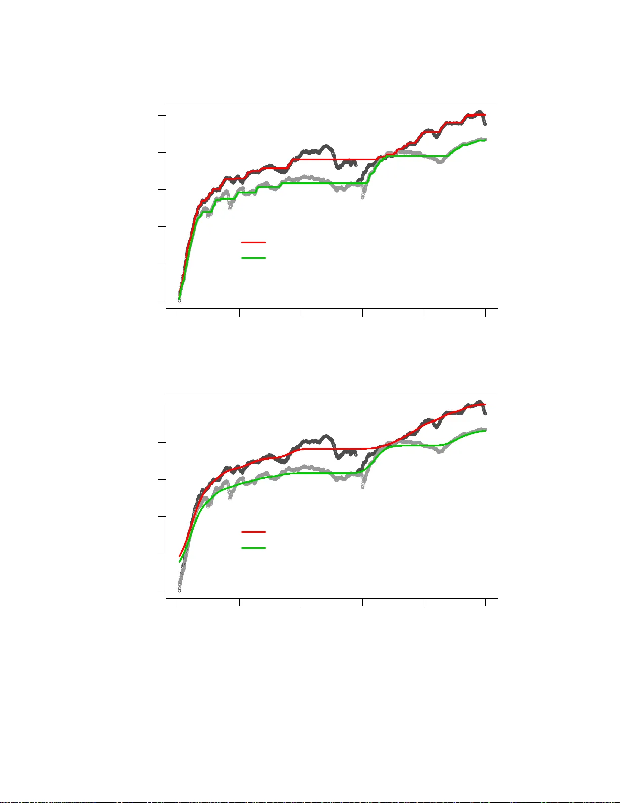
Least Squares estimatio n of two ordered monotone regression curves Fadoua Balabdaoui (1 , 2) , Kaspar Rufibach (3) and Filippo Santambrogio (1) 1 CEREMADE Univ ersit ´ e de Paris-Dauphine Place du Mar ´ echal de Lattre de T assigny 75775 Paris CEDEX 16, France 2 Univ ersit ¨ at G ¨ ottingen Institut f ¨ ur Mathematische Stochastik Goldschmidt strasse 7 37077 G ¨ ot tingen 3 Univ ersit ¨ at Z ¨ urich Institut f ¨ ur Sozial- und Pr ¨ aventivmedizin Abteilung Biostatistik Hirschengraben 84 8001 Z ¨ urich November 10, 2018 Abstract In this paper , we consider the p roblem of findin g the Least Squares estimator s of two isoton ic regression curves g ◦ 1 and g ◦ 2 under the additional constraint that they are ordere d; e .g., g ◦ 1 ≤ g ◦ 2 . Giv en two sets of n data points y 1 , . . . , y n and z 1 , . . . , z n observed at (the same) design points, the esti- mates of the tru e curves are obtain ed by minim izing the weigh ted Least Squares criter ion L 2 ( a, b ) = P n j =1 ( y j − a j ) 2 w 1 ,j + P n j =1 ( z j − b j ) 2 w 2 ,j over the class of pairs of v ectors ( a, b ) ∈ R n × R n such that a 1 ≤ a 2 ≤ . . . ≤ a n , b 1 ≤ b 2 ≤ . . . ≤ b n , and a i ≤ b i , i = 1 , . . . , n . The characterization of the estimators is established. T o comp ute th ese estimators, we use an iter ativ e pro jected subgrad ient algorithm , where the projection is perfo rmed with a “gen eralized” po ol-adjacen t-violaters algor ithm (P A V A), a byproduct of this work. Then, we app ly the estimation metho d to real d ata from mechan ical engineer ing. Ke ywords : least squares; m onoto ne regres sion; pool-adja cent-v iolaters algorit hm; shape constrain t esti- mation; subgrad ient algorithm 1 1 Introd uction and motivation Estimating a monotone regressio n curv e is one of the most class ical estimati on probl ems under shape re- stricti ons, see e.g. B runk (1958). A re gress ion curv e is said to be is otonic if it is mo notone nonde creasin g. W e chose in this paper to look at the class of isotonic reg ressio n functions. The simple transfor mation g → − g suffices for the results of this pape r to carry ov er to the antit onic class. Giv en n fixed points x 1 , . . . , x n , assume that we observ e y i at x i for i = 1 , . . . , n . When the points ( x i , y i ) are join ed, the shape of the obta ined graph can hint at the increa sing monoton icity of the true reg ression curve, g ◦ say , assuming the model y i = g ◦ ( x i ) + ε i , with ε i the uno bserv ed errors. This shape restric tion can also be a feature of the scienti fic proble m at hand, and henc e the need for estimating the true curv e in the class of antiton ic functio ns. W e refer to Barlo w et al. (1972) and Robertson et al. (1988) for examp les. T he weighted Least Square s estimate of g ◦ in the class of isoton ic functi ons taking y i at x i is the uniqu e m inimizer of the criteri on L ( a ) = n X i =1 w i ( y i − a i ) 2 (1) ov er the class of vec tors a ∈ R n such that a 1 ≤ a 2 . . . ≤ a n where w 1 > 0 , w 2 > 0 , . . . , w n > 0 are gi ve n posi ti ve weights. In what foll o ws, we will say that a vect or v ∈ R n is increasing or isotoni c if v 1 ≤ . . . ≤ v n , and use the notati on v ≤ w for v , w ∈ R n if the inequ ality holds compon entwise. It is well kno wn that the solution a ∗ of the L east S quares prob lem in (1) is giv en by the so-called min -max formula; i.e., a ∗ i = max s ≤ i min t ≥ i Av ( { s, . . . , t } ) (2) where Av ( { s, . . . , t } ) = P t i = s y i w i / P t i = s w i (see e.g. Barlo w et al., 1972). v an Eeden (1957a,b) has genera lized this problem to inco rporate k no wn bounds on the regre ssion funct ion to estimat e; i.e., she consi dered minimization of L under the constraint a L ≤ a ≤ a U , (3) for two incr easing ve ctors a L and a U . As in the class ical setting, the soluti on of this problem admits also a min-max repr esenta tion. T he P A V A can be gener alized to ef ficientl y compute this solutio n and has been implemented in the R package OrdM onReg (Balabdaoui et al. , 2009). Computat ion relies on a suitab le functio nal M defined on the sets A ⊆ { 1 , . . . , n } which generalizes the function Av in (2). This functi onal for the bound ed monoton e regressi on in (3) is gi ven by M ( A ) =  Av ( A ) ∨ max A a L  ∧ min A a U where min A v = min i ∈ A v i and max A v = max i ∈ A v i . C ompare Barlo w et al. (1972, p. 57), where a functi onal notation is use d. Howe ve r , in the la tter refe rence no for mal justificat ion was gi ven for t he form of the funct ional M nor for the valid ity of (the m odified versio n of) the P A V A, see the disc ussion after Theorem 2.1. 2 Chakra varti (1989) discusses the bounded isotonic regressio n proble m for the absolut e valu e criterion functi on, yie lding the bounded isotonic med ian regress or . He propo ses a P A V A-like algorithm as well, and establ ishes some connectio ns to linear progr amming theory . Unbound ed isotonic median regres sion was first cons idered by Robertson and W altman (1968), who provide d a min-max formula for the estimator and a P A V A-like a lgorith m to compute it. They also stud ied its con sistenc y . No w suppo se that instead of ha ving only one set of observ ations y 1 , . . . , y n at the design points x 1 , . . . , x n , we are interest ed in analyz ing two sets of data y 1 , . . . , y n and z 1 , . . . , z n observ ed at the same design points . F urthermo re, if we hav e the informatio n that the underlyi ng true regr ession curve s are increasing and ordere d, it is natura l to try to constr uct estimato rs that fulfill the same constrain ts. The current paper presents a solution to this problem of estimating two isoton ic regres sion curv es under the addition al constr aint that they are ordered. This soluti on is the unique m inimizer ( a ∗ , b ∗ ) of the criteri on L 2 ( a, b ) = n X i =1 w 1 ,i ( y i − a i ) 2 + n X i =1 w 2 ,i ( z i − b i ) 2 (4) ov er the class of pairs of vec tors ( a, b ) ∈ R n × R n such that a and b are increasin g and a ≤ b , with w 1 and w 2 gi ve n vecto rs of positi ve weights in R n . The proble m was moti v ated by an app licatio n from mechani cal engineerin g. W e will mak e use of e xpe ri- mental data obtain ed from dynamic material tests (see Shim and Mohr, 2009 ) to illustr ate our estimation method. In engineering mechanics, it is common practi ce to determine the deformation resistance and streng th of materials from uniaxial compression tests at dif feren t load ing velocitie s. The experime ntal results are the so-calle d stress-strai n curv es (see Figure 1), and these may be used to deter mine the de- formatio n resistan ce as a function of the applied deformation . The recorded signal s contain subs tantial noise which is mostly due to v ariatio ns in the loading veloc ity and electri cal noise in the data acqui sition system. The data in this e xampl e consis t of 1495 dist inct pairs ( x i , y i ) and ( x i , z i ) w here x i is the measu red s train, while y i (gray curv e) and z i (black curve ) correspond to the exp erimenta l stress results for two dif fere nt loadin g velocit ies. The true regres sion curves are expec ted to be (a) monoto ne increasing as the stress is kno wn to be an increasing functio n of the strain (for a giv en constant loadin g velocit y), and (b) ordered as the deformatio n resistance typic ally increases as the loading velocity increases. In Section 3, we sho w the resulti ng estimates as well as a smoothe d version thereof . W e will show th at minimizing L 2 is equi v alen t to minimizing anothe r con ve x functional over the cl ass of isoton ic v ector s a ∈ R n . B y doing so, we redu ce a two-curv e proble m un der the cons traints o f monotonic - ity and o rdering to a o ne-cur ve problem under the co nstrai nt of mono tonic ity and bou ndedn ess. A ctually , we can ev en perfo rm the minimization o ver the class of isotonic vectors ( a 1 , . . . , a n − 1 ) of dimension n − 1 satis fying the cons traint a 1 ≤ . . . ≤ a n − 1 ≤ a ∗ n as w e can explici tly determine a ∗ n by a gen- era lized min-max formula (see Proposition 2.3 ). The solutio n of this equi v alent minimization problem, which gi v es the solution a ∗ (and also b ∗ becaus e it is a function of a ∗ ), is computed usin g a projecte d subgra dient algorith m where th e pro jection ste p is perfo rmed using a sui table ge neraliz ation of the P A V A. 3 0.0 0.2 0.4 0.6 0.8 1.0 0 5 10 15 20 25 measured strain, x stress Figure 1: Original observ atio ns. Alternati vely , the so lution can be compu ted usin g Dykstra’ s algorithm (Dykstra, 1983). This point will be furthe r discu ssed in Section 3. W e would like to note that Brunk et al. (1966) consid ered a related problem, that of nonpara metric Max- imum likeli hood estimation of two ordered cumulati ve distrib ution functions . I n the same class of prob- lems, Dykstra (1982) treated estimation of surviv al functions of two stochasti cally ordered random vari - ables in the presence of censoring , w hich was extende d by F eltz and Dykstra (1985) to N ≥ 2 stochasti - cally ordere d random varia bles. The theore tical solution can be related to the well-kno wn Kaplan-Meier estimato r a nd can be computed using a n iterati ve algorithmic proce dure for N ≥ 3 (see Feltz and Dykstra, 1985, p. 1016). The √ n − asymptotics of the estimat ors for N = 2 , whether there is censo ring or not, were estab lished by Præstgaard and Huang (199 6). The paper is orga nized as follows. In Section 2, we giv e the charact erizati on of the ordered isotonic estimates . W e also provid e the expli cit form of the soluti on of the related bounded isotonic reg ressio n proble m where the uppe r of the two isot onic curve s is assumed to be fully kno wn. In Section 3 we describ e the projected sub gradie nt algorith m that we use to comput e the Least Squa res e s- timators of the ordered isoton ic re gres sion curv es, discu ss th e connection to Dykstra ’ s a lgorith m (Dykstr a, 1983), and apply the method to real data from mechanica l enginee ring. The technic al proofs are deferred to appe ndices A and B. 4 2 Estimation of two order ed isotonic r egr ession cur ves If the l ar ger of the two isoton ic curv es wa s k no wn, then there w ould of c ourse b e n o ne ed to estimate it. If we put a U = a 0 , th e weighted Least Squ ares estimate a ∗ of th e smaller isoto nic curve is the mini mizer of L ( a ) = n X i =1 w i ( y i − a i ) 2 , where w ∈ R n is a vector of giv en positi ve w eights, and a ∈ I a 0 n , the class of isotonic vectors a ∈ R n such that a ≤ a 0 and a 0 ∈ R n . W hen the compone nts of a 0 are a ll equal, the vector a 0 will be assimila ted with the common v alue of its componen ts as done in Proposi tion 3.4 below . The notatio n I w n will be used again hereafter to denote the class of isotonic vectors v ∈ R n such that v ≤ w . The statemen t of Barlo w et al. (197 2, p. 57) implies that if we define M ( A ) = Av ( A ) ∧ min A a 0 for a subset A ⊆ { 1 , . . . , n } , then the solutio n a ∗ can be computed using an appropria tely modified ver sion of the P A V A . Theor em 2.1. F or i = 1 , . . . , n , we have a ∗ i = max s ≤ i min t ≥ i M ( { s, . . . , t } ) = max s ≤ i min t ≥ i  Av ( { s, . . . , t } ) ∧ a 0 s  . T o keep this paper at a reasonabl e length, the proof of Theorem 2.1 is omitted. A short note contai ning a more thoro ugh discussi on of the one-cu rve problem an d a proof o f Theorem 2.1 can be o btaine d from the author s upon request. A general descrip tion of the modified P A V A an d a proo f that it work s whene ver th e functi onal M satisfies the so-called A ver agi ng Pr opert y can be found in Section 3. W e now retu rn to the main subject of this pape r . Theorem 2.1 is crucial for finding the Least Squares estimates of two ordered isotonic regre ssion curv es. In partic ular , the result will be used to de velo p an approp riate algori thm to compute the solution. Let y 1 , . . . , y n and z 1 , . . . , z n be th e observ ed data from tw o unkno wn isoto nic curv es g ◦ 1 and g ◦ 2 such th at g ◦ 1 ≤ g ◦ 2 . Giv en two v ectors in R n of positi ve weights w 1 and w 2 , we would lik e to minimize (4) ov er the class of pairs of vect ors ( a, b ) ∈ R n × R n such that a and b are isoton ic and a ≤ b . Call this class I n . Existence and uniqueness of t he solutio n. They follo w from con v exit y and clo sednes s of I n and stri ct con ve xity of L 2 . Characteri zation of the solution. F or completenes s, we gi v e the characteriza tion of the solution of minimizing (4) ov er I n ; i.e, a necessa ry and suf ficient condition for ( a, b ) ∈ I n to be equal to this soluti on. Let i 1 < . . . < i k such that i 1 = 1 , i k = n and a ∗ 1 = . . . = a ∗ i 1 < a ∗ i 1 +1 = . . . = a ∗ i 2 − 1 < . . . < a ∗ i k = . . . = a ∗ n . 5 W e call B 0 i j (resp. B 1 i j ) a set of indices { i j , . . . , i j +1 − 1 } , j = 1 , . . . , k − 1 such that a ∗ i j = b ∗ i j (resp. a ∗ i j < b ∗ i j ). Similarly , let l 1 < . . . < l r such that l 1 = 1 , l r = n such that b ∗ 1 = . . . = b ∗ l 1 < b ∗ l 1 +1 = . . . = b ∗ l 2 − 1 < . . . < b ∗ l k = . . . = b ∗ n and call C 0 l j (resp. C 1 l j ) a set of indices { l j , . . . , l j +1 − 1 } , j = 1 , . . . , r − 1 such that b ∗ l j = a ∗ l j (resp. b ∗ l j > a ∗ l j ). Theor em 2.2. The pair ( a ∗ , b ∗ ) ∈ I n is the minimizer of (4) if and only if n X i =1 ( a ∗ i − y i )( a ∗ i − a i ) w 1 ,i + n X i =1 ( b ∗ i − z i )( b ∗ i − b i ) w 2 ,i ≥ 0 , ∀ ( a, b ) ∈ I n (5) X s ∈∪ j B 1 i j ( a ∗ s − y s ) a ∗ s w 1 ,s = 0 , and (6) X s ∈∪ j C 1 l j ( b ∗ s − z s ) b ∗ s w 2 ,s = 0 . (7) Pr oof. See Appendix A. An explicit formula in the sense of a min-max represen tation similar to (2 ) of ( a ∗ , b ∗ ) turned out be to hard to find. Howe v er , since a ∗ (resp. b ∗ ) is also the minimizer of n X i =1 ( a − y i ) 2 w 1 ,i  resp. n X i =1 ( b − z i ) 2 w 2 ,i  ov er the clas s I b ∗ n (resp. the class of isotonic vector s b ∈ R n such that b ≥ a ∗ ), Theore m 2.1 implies that a ∗ i = max s ≤ i min t ≥ i ( Av 1 ( { s, . . . , t } ) ∧ b ∗ s ) (8) b ∗ i = max s ≤ i min t ≥ i ( Av 2 ( { s, . . . , t } ) ∨ a ∗ t ) (9) for i = 1 , . . . , n , where Av 1 ( A ) = P i ∈ A y i w 1 ,i P i ∈ A w 1 ,i , and Av 2 ( A ) = P i ∈ A z i w 2 ,i P i ∈ A w 2 ,i for A ⊆ { 1 , . . . , n } . Thus, the soluti on ( a ∗ , b ∗ ) is a fixed p oint of the operato r P : I n → I n defined as P (( a, b )) = ( P 1 ( b ) , P 2 ( a )) (10) =  max s ≤ i min t ≥ i ( Av 1 ( { s, . . . , t } ) ∧ b s ) , m ax s ≤ i min t ≥ i ( Av 2 ( { s, . . . , t } ) ∨ a t )  . Ho wev er , this fixed point problem does not admit a unique soluti on. Therefore, there is no guaran tee that an algorithm based on the abov e min-max formulas yields the solution, exc ept in the unrealist ic and 6 uninte resting case where the starting point of the algorithm is the solution itself. T o see that P does not admit a unique fixed p oint, note that the minimizer of the criterion n X i =1 ( a i − y i ) 2 w 1 ,i + B n X i =1 ( b i − z i ) 2 w 2 ,i is a fixed poin t of P for any B > 0 . Therefore, a computa tional method based on startin g from an initia l candid ate and then alternatin g between (8) and (9) cannot be success ful. In parallel, we hav e in vested a substa ntial ef fort in trying to get a closed form for the estimators. Although we did not succeed, we were able to obtain a closed form for a ∗ 1 (and by symmetry for b ∗ n ). Pro position 2.3. W e have that a ∗ 1 = min t ≥ 1 Av 1 ( { 1 , . . . , t } ) ∧ min t ≥ t ′ ≥ 1 ˜ M ( { 1 , . . . , t } , { 1 , . . . , t ′ } ) wher e ˜ M ( A, B ) = Av 1 ( A )( P i ∈ A w 1 ,i ) + Av 2 ( B )( P j ∈ B w 2 ,j ) P i ∈ A w 1 ,i + P j ∈ B w 2 ,j . By symmetry , we also have that b ∗ n = max t ≤ n Av 2 ( { t, . . . , n } ) ∨ m ax t ≤ t ′ ≤ n ˜ M ( { t ′ , . . . , n } , { t, . . . , n } ) . (11) Some remarks are in order . The expre ssions obtained abo v e indi cate that the Least Squares estimat or must depend, as expe cted, on the relati v e ratio of the weights w 1 and w 2 . In particula r , if w 2 = 0 (resp. w 1 = 0 ), the expres sion of a ∗ 1 (resp. b ∗ n ) speciali zes to the well-kno wn min-max formula in the classical Least Squares estimati on of an (unbounded ) isotonic curve. The ex pressi on of b ∗ n is essent ial for our subgra dient algori thm below . Pr oof of Pr opos ition 2.3. S ee Append ix A. In the ne xt sect ion, we describe ho w w e can make use of the min-max formula in (8) to compute the estimato rs usin g a proje cted subgradien t algorithm. As mentioned abo ve , we use in this algorithm the identi ty (11) gi ve n in the pre vious propositi on. 3 Algorithms and A pplication to r eal data In this section, we sho w that the bounded isotonic estimato r can be computed u sing the w ell-kn o wn P A V A, or to b e more p recise a mod ified ve rsion of it. Recall that the bo unded isoton ic estimator in the one- curv e proble m is gi v en by a ∗ i = max s ≤ i min t ≥ i M ( { s, . . . , t } ) 7 where M ( A ) = Av ( A ) ∨ max A a 0 for any A ⊆ { 1 , . . . , n } . That a ∗ can be computed using a P A V A is a cons equenc e of a more gene ral result. Namely , that a funct ional M of sets A ⊆ { 1 , . . . , n } satisfies what is referr ed to as the A ver ag ing Pr ope rty , (see Chakra varti, 1989, p. 138), also called Cauchy Mean V alue Pr operty by Leurga ns (1981, S ection 1). See also Robertson et al. (1988, p. 390). Note that in the classical unconstra ined monotone regre ssion problem, the min-max expre ssion of the Least Squares estimato r follo ws from Theorem 2.8 in Barlo w et al. (1972, p. 80). 3.1 Getting the min-max solution by the P A V A First, let us descr ibe ho w the P A V A wo rks for some set functio nal M . • At ev ery step the current configurat ion is gi v en by a subdi vision of { 1 , . . . , n } into k subsets S 1 = { 1 , . . . , i 1 } , S 2 = { i 1 + 1 , . . . , i 2 } , . . . , S k = { i k − 1 + 1 , . . . , n } for some indices 1 = i 0 ≤ i 1 < i 2 < · · · < i k − 1 < i k = n . • The initial configura tion is gi v en by the finest subdi vision; i.e., I j = { j } . • At ev ery step w e look at the valu es of M on the sets of the subdi visi on. A violati on is noted each time there exists a v alue j such that M ( S j ) > M ( S j +1 ) . W e consider the first violatio n (the one corres pondin g to the smallest j ) and then mer ge the subs ets S j and S j +1 into one interv al. • Giv en a new subdi vision (which has one subset less than the prev ious one), we look for possible violat ions. • The algori thm stops when there are no violatio ns left. Since for any violation a mer ging is performed (thus reducing the number of subsets), it is clear that the algori thm stops after a finite number of iterati ons. W e require now the set function al M to satisfy the follo wing property . See L eur gan s (1981, Section 1), Robertso n et al. (1988, p. 390) and Chakra v arti (1989, p. 138). Definition 3.1. W e say that the functional M sati sfies the A verag ing Pr ope rty if for any sets A and B suc h that A ∩ B = ∅ w e have that min { M ( A ) , M ( B ) } ≤ M ( A ∪ B ) ≤ max { M ( A ) , M ( B ) } . If h and w > 0 are giv en vecto rs ∈ R n , then besi de A 7→ Av ( A ) = X i ∈ A w i h i / X i ∈ A w i , 8 the follo w ing examples of funct ions also satisfy the A verag ing P roperty : A 7→  Av ( A ) ∨ max A h 1 i  ∧ min A h 0 , with h 0 , h 1 two v ectors ∈ R n , A 7→ min A h = min i ∈ A h i , A 7→ med A h = arg min m ∈ R X i ∈ A | h i − m | w i where the arg min is tak en to be the smallest m in case non-uni quene ss occurs , A 7→ max A h = max i ∈ A h i . Note that the maximum, the minimum and the sum of two functi onals satisfying the A ve raging Property satisfy the same prop erty as well. Theor em 3.2. The final configur atio n obtained by the P A V A is such tha t the two followin g pr ope rties ar e satisfi ed. 1. The func tional M is incr eas ing on the sets of the subdi vision . 2. If one of the sets S j = C ∪ D is the disjoint unio n of two subse ts C = { i j − 1 + 1 , . . . , k } and D = { k + 1 , . . . , i j } , then M ( C ) > M ( D ) ; i.e., a finer subdi vision would necess arily cau se a violat ion. Pr oof. The fac t that M is increa sing on the final configuration is an easy consequenc e of the absenc e of violat ions (otherwise the algorit hm would not hav e stoppe d). As for th e second part of th e prope rty , note that this is sa tisfied by the in itial configura tion (since no set is the disjoint union of two non-t ri vial subsets), as w ell as by any configurat ion that one could obtain after the fi rst mergi ng (since a m er ging occurs only because of a violat ion). No w we will use an inducti ve reason ing. T o th is end, we hav e to chec k two situat ions: Suppose we merg e two subsequent sets A and B and want to check whethe r there is a v iolatio n on C and D , with A ∪ B = C ∪ D . W e are in one of the two followin g cases: either A = A 1 ∪ A 2 , C = A 1 and D = A 2 ∪ B , o r B = B 1 ∪ B 2 , C = A ∪ B 1 and D = B 2 (the case C = A and D = B is triv ial). In the first case, if we supp ose M ( D ) ≥ M ( C ) , we get M ( A 2 ∪ B ) ≥ M ( A 1 ) , M ( A 2 ) < M ( A 1 ) , M ( B ) < M ( A ) = M ( A 1 ∪ A 2 ) , (the first inequality follo ws by assumption , the second by inductio n, and the third is true since A and B ha ve bee n merged) and this is impossi ble since one wou ld conclud e that max { M ( A 2 ) , M ( B ) } ≥ M ( A 1 ) > M ( A 2 ) , and hence M ( A ) > M ( B ) ≥ M ( A 1 ) > M ( A 2 ) , which implies M ( A ) > max { M ( A 1 ) , M ( A 2 ) } , which contra dicts the A veragin g Property . 9 In the secon d case we wou ld ha ve M ( A ∪ B 1 ) ≤ M ( B 2 ) , M ( B 2 ) < M ( B 1 ) , M ( A ) > M ( B ) = M ( B 1 ∪ B 2 ) , which implies min { M ( A ) , M ( B 1 ) } ≤ M ( B 2 ) < M ( B 1 ) , and then min { M ( A ) , M ( B 1 ) } = M ( A ) and M ( A ) ≤ M ( B 2 ) < M ( B 1 ) , which contradic ts eithe r M ( A ) < M ( B ) or the A verag ing Property . ✷ Theor em 3.3. If ( S j ) j is the partition obtain ed at the end of the P A V A describe d abo ve , then m i = M ( S j i ) suc h that i ∈ S j i tak es the same values given by the min-max formu la for the index i . Pr oof. See Appendix A. 3.2 Shor’ s projected subgradient and Dykstra’ s i terativ e cyclic pr ojection algorithm The minimizatio n problem consid ered in th is pape r can b e eas ily reco gnized as a projection proble m onto the interse ction of the three follo wing closed con ve x cones in R n × R n { ( a, b ) : a is increasing } , { ( a, b ) : b is increasing } , and { ( a, b ) : a ≤ b } . Projectio ns on to the fi rst two cones can b e computed by P A V A , and onto the la st one by replacing the componen ts of each pair ( a i , b i ) violatin g the constrain t (i.e. a i > b i ) by the weighted ave rage ( w 1 ,i a i + w 2 ,i b i ) / ( w 1 ,i + w 2 ,i ) of a i and b i . Implementa tion of D ykstra’ s algorith m (Dykstra, 1983) is then straig htforw ard. Y et, our algorithm has preferable features as we will now ex plain. The algori thm de ve lopped by Dykstra is well-suite d for projectio ns onto intersection s of con vex sets or half-spaces (see Bregman et al., 2003), while the algorithm w e propos e can handle a larg er class of minimizatio n proble ms which in volv e the set of isoto nic vecto rs, and are not necessarily projections . For instance, simple modifications of our algori thm would allo w us to minimize any objecti ve function of the form ( a, b ) 7→ F ( a, w 1 ) + n X i =1 w 2 ,i ( z i − b i ) 2 under the same constrain ts on a and b , where F is any con vex and dif ferent iable function. T he second quadra tic term can b e als o rep laced by a d if feren t penali zation term dep endin g e.g. on an L p -distan ce. In- deed, it suf fices to modify the computa tions in v olv ed in t he P A V A by a daptin g them to var ious fu nction als satisfy ing the A veragin g P roperty (see Section 3). Our algorit hm is eas y to understan d and is only b ased on a classical grad ient method. Once the min imiza- tion is perfo rmed with resp ect to on e of th e v ariabl es, the object i ve funct ion with res pect to th e remainin g v ariabl e is still explic it, b ut no more diff erentia ble. This is the main reason for which the algorith m is actual ly a subgra dient descen t. W e belie ve that the exp licit nature of the computat ions in our subgr adient algori thm are exa ctly the key feature for the possibi lity of unders tandin g and/or modifyin g it. 10 Ho wev er , we woul d like to point out the m erits of Dykstra’ s algorithm in this specific setting. S ince it is tailore d for a Least S quares problem, and becaus e only three very simple projection cones are in vol ved , Dykstra’ s algorith m (see belo w for details) computes the minimum of the criterio n L 2 gi ve n in (4) faster than the subgr adient algorith m, altho ugh Dykstra’ s algorithm is typi cally consid ered to be rather slo w (see e.g. Mammen, 1991 a or Birke and Dette, 200 7). Note that the choice of th e stopp ing criterion in this algori thm m ay be delica te, see Bir gin and Raydan (2005). Howe v er , this was not an issue in our setting. 3.3 Pr eparing for a pr ojected subgradient algorithm The follo w ing propos ition is c rucial for computing the o rdered iso tonic estimat ors via a pr ojected sub gra- dient algorith m. Pro position 3.4. Let Ψ be the criter ion Ψ( b 1 , . . . , b n − 1 ) = n X i =1  max s ≤ i ( G s,i ∧ b s ) − y i  2 w 1 ,i + n − 1 X i =1 ( b i − z i ) 2 w 2 ,i (12) which is to b e minimized on the con vex set I b ∗ n n − 1 = { ( b 1 , . . . , b n − 1 ) ∈ R n − 1 : b 1 ≤ b 2 ≤ . . . ≤ b n − 1 ≤ b ∗ n } wher e G s,i = min t ≥ i Av 1 ( { s, . . . , t } ) and b n = b ∗ n in (12) . The criter ion Ψ is con ve x. Furthermor e, its unique minimizer ( b ∗∗ 1 , . . . , b ∗∗ n − 1 ) equals ( b ∗ 1 , . . . , b ∗ n − 1 ) . Pr oof. Let us write I = I ∞ n = { a = ( a 1 , . . . , a n ) ∈ R n : a 1 ≤ . . . ≤ a n } , I ∗ n = n b = ( b 1 , . . . , b n ) : ( b 1 , . . . , b n − 1 ) ∈ I b ∗ n n − 1 and b n = b ∗ n o and consid er I b n = { a : a ∈ I and a ≤ b } for b ∈ I ∗ n . No w note that the min-max formula in (8) allo w s us to write n X j =1  max s ≤ j ( G s,j ∧ b s ) − y j  2 w 1 ,j + n − 1 X j =1 ( b j − z j ) 2 w 2 ,j = min a ∈I b n n X j =1 ( a j − y j ) 2 w 1 ,j + n − 1 X j =1 ( b j − z j ) 2 w 2 ,j . 11 Hence, we ha v e for b ∈ I ∗ n Ψ( b 1 , . . . , b n − 1 ) = min a ∈I b n n X j =1 ( a j − y j ) 2 w 1 ,j + n − 1 X j =1 ( b j − z j ) 2 w 2 ,j = n X j =1 (˜ a j ( b ) − y j ) 2 w 1 ,j + n − 1 X j =1 ( b j − z j ) 2 w 2 ,j where ˜ a j ( b ) = max s ≤ j ( G s,j ∧ b s ) is the j -t h compo nent of the m inimizer of the functio n P n j =1 ( a j − y j ) 2 w 1 ,j in I b n . Let λ ∈ [0 , 1] , and b and b ′ in I ∗ n . By definition of I b n and I b ′ n , we ha v e that λ ˜ a ( b ) + (1 − λ ) ˜ a ( b ′ ) ≤ λ b + (1 − λ ) b ′ and hence n X j =1  ˜ a j ( λ b + (1 − λ ) b ′ ) − y j  2 w 1 ,j ≤ n X j =1  λ ˜ a ( b ) + (1 − λ ) ˜ a ( b ′ ) − y j  2 w 1 ,j ≤ λ n X j =1  ˜ a j ( b ) − y j  2 w 1 ,j + (1 − λ ) n X j =1  ˜ a j ( b ′ ) − y j  2 w 1 ,j . This shows con vexity of the first term of Ψ . C on ve xity of Ψ now follo ws from con vexit y of the function P n − 1 j =1 ( b j − z j ) 2 w 2 ,j and t he fac t tha t the sum of two con vex fun ctions defined on the s ame doma in is also con ve x. ✷ The idea behin d considering the con vex functional Ψ is to reduce the dimensionality of the problem as well as the number of constr aints (from 3 n − 2 to n − 1 con straint s). Once Ψ is minimized ; i.e, the isoton ic estimate b ∗ is computed, a ∗ can be obtaine d using the min-max formula giv en in (8). H o we ver , the con ve x functional Ψ is not continu ously dif ferenti able, hence the need for an optimizati on algorithm that uses the subgr adient inste ad of the gradie nt as the latter is no t defined ev erywhere. 3.4 A pr ojected subgradient algorithm to compute b ∗ 1 , . . . , b ∗ n − 1 T o minimize the non-smooth con ve x functio n Ψ we use a projected subgrad ient algorit hm. Since the gradie nt does not exi st on the entire domain of the funct ion, one has to resort to computation of a sub- gradie nt, the analogue of the gradien t at point s where the latter does not exis t. As oppose d to clas sical methods de v eloped for minimizing smooth function s, the procedure of searchi ng for the directio n of de- scent and steplen gths is entirely differe nt. The classica l reference for subgrad ient algorithms is S hor (1985). Boyd et al. (2 003) pro vide a n ice summary o f the topi c, including the p rojecte d varian t. Note th at a recen t applica tion in statistic s of the subgra dient algorithms gi ve s no w the possibil ity to compute the log-co nca v e density estimator in high dimensions ; see Cule et al. (2008). 12 The main steps of the algorithm. No w recall that the functional Ψ should be minimized over the ( n − 1) − dimens ional co n vex set I b ∗ n n − 1 gi ve n in Proposi tion 3.4. Of co urse, t his is the s ame as minimizing Ψ ov er the n − dimension al con v ex set { ( b 1 , . . . , b n ) | b 1 ≤ . . . ≤ b n − 1 } , starting with an initial vector ( b (0) 1 , . . . , b (0) n ) such that b (0) n = b ∗ n and constrai ning the n − th component of the sub-gradi ent of Ψ to be equal to 0. Giv en a ste pleng th τ k , the ne w iterate b k +1 = ( b k 1 , . . . , b k n ) at the k − th iterat ion o f a subgr adient a lgorith m is gi v en by v k +1 = b k − τ k D k , where D k is the subgradien t calcu lated at the previo us iterate; i.e., D k = ˜ ∇ Ψ( v k ) (see Appendix B). Ho wev er , it m ay happen that v k +1 is not admissible; i .e. ( b k +1 1 , . . . , b k +1 n − 1 ) does not belong to I b ∗ n n − 1 . When this occurs, an L 2 projec tion of this iterate onto I b ∗ n n − 1 is performed. This is equi v alent to finding the minimizer of n X i =1 ( a i − b k +1 i ) 2 ov er the set I b ∗ n n . The latter problem can be solv ed using the generalize d P A V A for bounded isotoni c reg ression as describ ed abov e. The computat ion of th e sub gradie nt D k is de scribed in detail in Append ix B. As for th e ste plengt h τ k , we start the algorithm with a cons tant steple ngth. Once a pre -specified numb er of it eration s has been re ached we switch to τ k +1 = ( h 0 . 1 k k D k k 2 ) − 1 where γ k := h − 0 . 1 k is suc h that 0 ≤ γ k → 0 as k → ∞ and P ∞ k =1 γ k = ∞ . Here, k · k 2 denote s the L 2 -norm of a vector in R n . T his combination of constan t and non-su mmable diminishing steplength sho wed a go od perfo rmance in our implemen tation of the alg orithm ov er oth er classica l choices of ( γ k ) k . Furthermor e, con ver gence is ensured by the followin g theorem. Theor em 3.5. (Boyd et al. (2003)) A subgr adient algorithm complemente d with least-sq uar e pr oje ction and using non-su mmable diminishing steplen gth yields for any η > 0 after k = k ( η ) iteratio ns a vector b k := ( b k 1 , . . . , b k n ) suc h that min i =1 ,...,k Ψ( b i ) − Ψ ( b ∗ ) ≤ η, wher e b ∗ = ( b ∗ 1 , . . . , b ∗ n ) is the vector given in Pr oposition 3.4. The proo f can be found in Boyd et al. (2003) by combinin g their argu ments in Sections 2 and 3. N ote that in our implementati on w e do not keep track of the iterat e that yielded the minimal value of Ψ , since we apply a problem-moti v ated stoppin g crite rion that guarantees us to ha ve reached an iterate that is suf ficient ly close to b ∗ = ( b ∗ 1 , . . . , b ∗ n ) . 13 Choice of stopping rule. Since in subgradien t algorith ms the con ve x tar get functiona l does not nec- essaril y monot onicall y decreas e with increasing number of iterati ons, the choice of a suita ble stopping criteri on is delicat e. Ho we ver , in our specific settin g w e use the fac t that ( a ∗ , b ∗ ) is a fi xed point of the operat or P defined in (10) where a ∗ = P 1 ( b ∗ ) ; the solution of (1) with upper bound b ∗ . This motiv ates iterati ng the algorit hm until the dif ference of entrie s of the two v ectors b k and b k # where b k # = P 2 ◦ P 1 ( b k ) is belo w a pre-spec ified positi ve constant δ . The implementation. T he Dykstra and the pr ojecte d subgrad ient alg orithms as wel l as the g ener - alized P A V A for computing the solut ion in the one curv e problem under the constraints in (3) were all implemented in R (R Dev elop ment Core T eam, 2008). The correspond ing packag e OrdM onReg Balabdao ui et al. (2009) is a v ailabl e on CR AN. Note that the data analyzed in Section 3.5 is made av ail- able as a dataset in OrdMon Reg . T o conclu de this section on the algorithmic aspect s of our work, w e would lik e to mention the work by Beran and D ¨ umbgen (2009) who propose an acti v e set algorith m w hich can be tailored to solve the proble m gi ven in (4) for an arbitra ry number of order ed monotone c urve s. Howe ve r , Beran and D ¨ umbgen (2009) do not provide an analysis of the struc ture of the estimated curves such as characteriz ations and rather put their emphasis on the algorith mic dev elopmen ts of the problem. 3.5 Real data example fr om mechanical engineering W e would li ke to esti mate the stress -strain curves base d on the a v aila ble experi mental data for two d if fer - ent ve locity le ve ls (see Figure 1). The exp ected curv es hav e to be isotonic and ordered . T he data consist of 1495 pairs ( x i , y i ) and ( x i , z i ) . The v alues of the measured strain of the material (on the x -axis), are actual ly defined as ( − ) the logarithm of the ratio of the current ov er the initia l specimen length. The v alues are posit i ve and take the maximal v alue 1, which corresp onds to a maximum shorte ning of 63%. Furthermor e, since the stress measurements for dif fere nt vel ocities are not perfor med exactly at the same strain, th e v alues of the stre ss ha ve bee n int erpola ted at equ ally sp aced v alues of the strain. A s pointed out by a re feree, this will in duce correl ation between the strain d ata. E ven if t he strai n measurement were not interp olated, ha ving correlat ed stress m easure ments is rather inevita ble in this particular applicati on be- cause of the d ata proc essing procedur es associ ated with the measure ment techniqu e (see Shim and Mohr, 2009). The estimation method is ho we ver s till applica ble. When studyi ng statist ical properties of the iso - tonic estimat ors such as con sisten cy and con ver gence, the correlation between the data should, of course, be taken int o account. In such p roblems, pr actitio ners usuall y fit parametri c models using a trial and error appro ach in an attempt to capture monoton icity of the stress-str ain curves as well as their ordering. The methods used are rather arbitra ry and can also be time consuming , hence the need for an alte rnati ve estimation approach. Our main goal is to provide those practitione rs with a rigorous way for estima ting the ord ered stress-strai n curv es. 14 In Figure 2 (upper plot) we provid e the origin al data (black and gray dots) and the proposed ordered iso- tonic es timates a ∗ and b ∗ as de scribe d above . B eing ste p functi ons, the estimate d isotonic curv es are no n- smooth, a well kno wn dra wback of isoton ic regress ion, see among others Wright (1978) and Muker jee (1988). The latter author pionee red the combin ation of isotonizatio n foll o wed by kernel smooth ing. A thorou gh asymptotic analysis of the smoothe d isotoni zed and the isotonic smooth estimators was gi ve n by Mammen (1991b). Mukerje e (198 8, p. 743) shows that monotoni city of the re gress ion funct ion is preser ved by the smoothing operation if the used ker nel is log-conc a ve. Thus, we define our smoothed ordere d m onoto ne estimato rs by ˜ a ∗ h ( x ) = P n i =1 K h ( x − t ) a ∗ i P n i =1 K h ( x − x i ) and ˜ b ∗ h ( x ) = P n i =1 K h ( x − t ) b ∗ i P n i =1 K h ( x − x i ) for 0 ≤ x ≤ 1 . Fo r simplicity , we used the kern el K h ( x ) = φ ( x/h ) w here φ is the density function of a standard normal distrib ution which is clearly log-co nca v e. Figure 2 (lower plot) depicts the smoothed isoton ic estimates . W e set the bandwidth to h = 0 . 1 n − 1 / 5 ≈ 0 . 023 . Moti v ated by es timation of str ess-str ain curv es, an ap plicati on from mech anical engine ering, we consider in this pa per weighted Least Squa res esti mators in the probl em of estimati ng two orde red isotonic regre s- sion curves. W e provide charac terizat ions of the solution and descr ibe a project ed subgradient algorith m which can be used to compute this soluti on. A s a by-pr oduct, we show ho w an adaptatio n of the well- kno wn P A V A can be used to compute min-max estimators for any set funct ional satisfying the A veragin g Property . Ackno wledgements. The first au thor would like to th ank C ´ ecile Durot for s ome intere sting discu ssions around the subjec t. W e also thank JongMin Shim for hav ing made the data av ailable to us, a re vie wer for drawin g our attention to Dykstra ’ s algorith m, and another re vie w er for helpful remarks. Refer ences B A L A B D AO U I , F . , R U FI B A C H , K . and S A N TA M B R O G I O , F. (20 09). O r dMonRe g: Compute leas t squ ar es estimates of one boun ded or two or der ed isotonic r e gr ession curves . R package vers ion 1.0.2. B A R L OW , R . E ., B A RT H O L O M E W , D . J. , B R E M N E R , J . M . and B RU N K , H . D . (1972). Statis tical infer ence under or der r estrictions. The theory and appl ication of isotonic r e gr ession . John W ile y & Sons, London -Ne w Y ork-Sydne y . W ile y Series in Probability and Mathematica l Statistics. B ER A N , R . and D ¨ U M B G E N , L . (2009 ). Least squar es and shrinkage estimation under bimono tonici ty constr aints. Statistics and Computing, to appear . 15 0.0 0.2 0.4 0.6 0.8 1.0 0 5 10 15 20 25 measured strain, x stress upper isotonic estimate b* low er isotonic estimate a* 0.0 0.2 0.4 0.6 0.8 1.0 0 5 10 15 20 25 measured strain, x stress upper isotonic smoothed estimate b ~ * low er isotonic smoothed estimate a ~ * Figure 2: Original observ ations, isotonic and isotonic smoothed estimates. 16 B I R G I N , E . G . and R A Y DA N , M . (2005). Rob ust stoppin g criteria for Dykstra’ s algorit hm. SIAM J. Sci. Comput. 26 1405– 1414 (electr onic). B I R K E , M . and D E T T E , H . (2007). Estimating a con ve x function in nonpa rametric regres sion. Scand. J. Statis t. 34 384– 404. B OY D , S . , X I AO , L . and M U T A P C I R , A . (2003). Subgr adient methods. Lecture Notes, Stanford Uni v er - sity . URL http:/ /www. stanford.edu/class/ee392o/subgrad_method.pdf B R E G M A N , L . M . , C E N S O R , Y . , R E I C H , S . and Z E P K O W I T Z - M A L A C H I , Y . (2003) . Finding th e projec - tion of a point onto the intersection of con v ex sets via project ions onto half-spa ces. J. Appr ox. T heory 124 194–2 18. B RU N K , H . D . (1958) . O n the estimatio n of parameters restricted by inequa lities. Ann. Math. Statist. 29 437–4 54. B RU N K , H . D . , F R A N C K , W . E . , H A N S O N , D . L . and H O G G , R . V . (1966) . M aximum likeli hood estimatio n of the distri b utions of two stochastic ally ordered random v ariable s. J. Amer . Statist. Assoc. 61 1067–1 080. C H A K R A V A RT I , N . (1989). B ounde d iso tonic med ian re gre ssion. Comput. Sta tist. Dat a Anal. 8 135–1 42. C U L E , M . , S A M W O RT H , R . and S T E W A RT , M . (2008). Maximum lik elihoo d estima tion of a multidi- mension al log-conca ve density . URL http:/ /www. D Y K S T R A , R . L . (1982). Maximum likeliho od estimation of the survi val functio ns of stochasti cally ordere d random v ariabl es. J. Amer . Statis t. Assoc. 77 621– 628. D Y K S T R A , R . L . (1983). An algorithm for restric ted least square s regre ssion. J. Amer . Stati st. Assoc. 78 837–8 42. F E LTZ , C . J . and D Y K S T R A , R . L . (1985) . Ma ximum likelihoo d estimation of the survi v al functio ns of N stoch astical ly ordered random vari ables. J. Amer . Statist. Assoc. 80 1012–101 9. L E U R G A N S , S . (1981). The Cauchy mean v alue propert y and linear functions of order statistics. Ann. Statis t. 9 905–9 08. M A M M E N , E . (1991a) . Estimating a smooth monoto ne regr ession function. Ann. Statist . 19 724– 740. M A M M E N , E . (1991b) . E stimating a smooth monoto ne reg ression function . A nn. Statis t. 19 724 –740. M U K E R J E E , H . (1988). Monotone nonparame teric regress ion. Ann. Statist. 16 741–750. 17 P R Æ S T G A A R D , J . T. and H U A N G , J . (1996). Asymptotic th eory for n onpar ametric estimati on of surviv al curv es under order restrictio ns. Ann. Statist . 24 1679–1 716. R D E V E L O P M E N T C O R E T E A M (2008). R: A Langua ge and E n vir onment for Statistica l Computin g . R Found ation for Statistical Computing, V ienna, Austria. ISBN 3-90005 1-07-0 . URL http:/ /www. R- project.org R O B E RT S O N , T. and W A LTM A N , P . (1968). On estimating monotone parameters. Ann. Math. Statist 39 1030– 1039. R O B E RT S O N , T., W R I G H T , F. T. and D Y K S T R A , R . L . (1988). Or der re stricte d statisti cal infer ence . W iley Series in Probability and Mathematica l Statistics: Probability and Mathematica l Statistics, John W iley & Sons Ltd., Chicheste r . S H I M , J . and M O H R , D . (2009) . Using split h opkin son pressure bars t o per form lar ge st rain compr ession tests on polyurea at low , in termedia te an d high strain rates. Intern ationa l J ourna l of Impact Engineerin g 36 1116 – 1127 . S H O R , N . (1985). Minimizatio n Methods for Non-Dif fere ntiabl e Functions . S pringe r , Berlin. V A N E E D E N , C . (1957a). Maximum lik elih ood estimation of partia lly or completely ordered paramete rs. I. Nederl. Akad. W etensc h. Pr oc. Ser . A. 60 = Inda g . Math. 19 128–1 36. V A N E E D E N , C . (1957b ). Maximum lik elih ood estimation of par tially or compl etely ordered para meters. II. Nederl. Akad. W etensc h. Pr oc. Ser . A. 60 = Inda g. Math. 19 201–2 11. W R I G H T , F . T. (1978) . Estimatin g strictly increas ing regressi on function s. Jo urnal of the American Statis tical A ssocia tion 73 636– 639. URL http:/ /www. jstor.org/stable/2286615 A Proofs Pr oof of Theor em 2.2. S uppos e that ( a ∗ , b ∗ ) is the solution . For ǫ ∈ (0 , 1) , and ( a, b ) ∈ I n consid er the pair ( a ǫ , b ǫ ) ∈ R n × R n defined as a ǫ = a ∗ + ǫ ( a − a ∗ ) b ǫ = b ∗ + ǫ ( b − b ∗ ) . For i ≤ j ∈ { 1 , . . . , n } , we hav e a ǫ j − a ǫ i = (1 − ǫ )( a ∗ j − a ∗ i ) + ǫ ( a j − a i ) ≥ 0 b ǫ j − b ǫ i = (1 − ǫ )( b ∗ j − b ∗ i ) + ǫ ( b j − b i ) ≥ 0 . 18 Also, for i ∈ { 1 , . . . , n } w e ha ve a ǫ i − b ǫ i = (1 − ǫ )( a ∗ i − b ∗ i ) + ǫ ( a i − b i ) ≤ 0 . Hence, ( a ǫ , b ǫ ) ∈ I n , and 0 ≤ lim ǫ ց 0 1 ǫ ( L 2 ( a ǫ , b ǫ ) − L 2 ( a ∗ , b ∗ )) = n X i =1 ( a ∗ i − y i )( a i − a ∗ i ) w 1 ,i + n X i =1 ( b ∗ i − z i )( b i − b ∗ i ) w 2 ,i yieldi ng the inequa lity in (5). No w consi der the vec tors a ǫ and b ǫ such that for l = 1 , . . . , n a ǫ l = a ∗ l + ǫ a ∗ l 1 l ∈ B 1 i j b ǫ l = b ∗ l Let r ≤ s ∈ { 1 , . . . , n } . If r / ∈ B 1 i j and s / ∈ B 1 i j , then a ǫ s − a ǫ r = a ∗ s − a ∗ r ≥ 0 . If r ∈ B 1 i j and s / ∈ B 1 i j , then a ∗ s > a ∗ r and a ǫ s − a ǫ r = a ∗ s − a ∗ r + ǫa ∗ s > 0 for | ǫ | small enou gh. The same reasoning appli es if r / ∈ B 1 i j and s ∈ B 1 i j . Finally , if r, s ∈ B 1 i j , then a ǫ s − a ǫ r = 0 . No w , for r ∈ { 1 , . . . , n } , we hav e a ǫ r = a ∗ r ≤ b ∗ r if r / ∈ B 1 i j . Otherwise, a ǫ r = a ∗ r (1 + ǫ ) < b ∗ r if | ǫ | is small enough . Hence, ( a ǫ , b ǫ ) ∈ I n , and 0 = lim ǫ ց 0 1 ǫ ( L 2 ( a ǫ , b ǫ ) − L 2 ( a ∗ , b ∗ )) = n X r =1 ( a ∗ r − y r )1 r ∈ B 1 i j a ∗ r w 1 ,r . Summing up o v er all the sets B 1 i j yields t he ident ity in ( 6). W e can prove very simil arly the identity in (7 ). Con versel y , suppose that ( a ∗ , b ∗ ) ∈ I n satisfies the inequ ality in (5). For an y ( a, b ) ∈ I n , we ha v e L 2 ( a, b ) − L 2 ( a ∗ , b ∗ ) = 1 2 n X i =1 ( a i − a ∗ i ) 2 w 1 ,i + 1 2 n X i =1 ( b i − b ∗ i ) 2 w 2 ,i + n X i =1 ( a ∗ i − y i )( a i − a ∗ i ) w 1 ,i + n X i =1 ( b ∗ i − z i )( b i − b ∗ i ) w 2 ,i ≥ 0 . W e conclude that ( a ∗ , b ∗ ) is the solution of the minimization problem. ✷ Pr oof of Pr oposi tion 2.3 . L et ǫ > 0 and consider ( a, b ) ∈ R n × R n such that a i = a ∗ i − ǫ 1 i ∈{ 1 ,...,t } , t ∈ { 1 , . . . , n } b i = b ∗ i 19 for i = 1 , . . . , n . For small ǫ , ( a, b ) ∈ I n . Using the charact erizati on in Theorem 2.2, it follo w s that t X j =1 ( a ∗ j − y j ) w 1 ,j ≤ 0 implying that t X j =1 ( a ∗ 1 − y j ) w 1 ,j ≤ 0 , for t ∈ { 1 , . . . , n } or equi valen tly a ∗ 1 ≤ min t ≥ 1 Av 1 ( { 1 , . . . , t } ) . No w , cons ider ( a, b ) ∈ R n × R n such that a j = a ∗ j − ǫ 1 j ∈{ 1 ,...,t } , t ∈ { 1 , . . . , n } b j = b ∗ j − ǫ 1 j ∈{ 1 ,...,t ′ } , 1 ≤ t ′ ≤ t for j = 1 , . . . , n , with ǫ > 0 . For small ǫ , we ha v e that ( a, b ) ∈ I 2 , and henc e t X j =1 ( a ∗ j − y j ) w 1 ,j + t X j =1 ( b ∗ j − z j ) w 2 ,j ≤ 0 . It follo ws that t X j =1 ( a ∗ 1 − y j ) w 1 ,j + t ′ X j =1 ( a ∗ 1 − z j ) w 2 ,j ≥ 0 , that is a ∗ 1 ≤ min 1 ≤ t ′ ≤ t ≤ n ˜ M ( { 1 , . . . , t } , { 1 , . . . , t ′ } ) . W e conclude that a ∗ 1 ≤ min t ≥ 1 Av 1 ( { 1 , . . . , t } ) ∧ min t ≥ t ′ ≥ 1 ˜ M ( { 1 , . . . , t } , { 1 , . . . , t ′ } ) . No w if a ∗ 1 < b ∗ 1 , let i 1 { 1 , . . . , n } be such that a ∗ 1 = . . . = a ∗ i 1 . Then ( a, b ) is such that a j = a ∗ j + ǫ 1 j ∈{ 1 ,...,i 1 } b j = b ∗ j for j = 1 , . . . , n is in I n when | ǫ | is small enough . It follo ws that Av 1 ( { 1 , . . . , i 1 } ) = a ∗ 1 . 20 If a ∗ 1 = b ∗ 1 , and i ′ 1 and i ′′ 1 are such that a ∗ 1 = . . . = a ∗ i ′ 1 and b ∗ 1 = . . . = b ∗ i ′′ 1 , then ( a, b ) such that a j = a ∗ j + ǫ 1 j ∈{ 1 ,...,i ′ 1 } b j = b ∗ j + ǫ 1 j ∈{ 1 ,...,i ′′ 1 } for j = 1 , . . . , n is in I n for | ǫ | small enough. Hence, a ∗ 1 = ˜ M ( { 1 , . . . , i ′ 1 } , { 1 , . . . , i ′′ 1 } ) . (note that i ′′ 1 ≤ i ′ 1 ). T herefo re, a ∗ 1 = min t ≥ 1 Av 1 ( { 1 , . . . , t } ) ∧ max t ≥ t ′ ≥ 1 ˜ M ( { 1 , . . . , t } , { 1 , . . . , t ′ } ) . The ex pressi on of b ∗ 1 follo w s easily by replacing respecti vely y i and z i by − z n − i +1 and − y n − i +1 for i = 1 , . . . , n . ✷ Pr oof of Theor em 3.3. Consider a ∈ R n gi ve n by a i = max s ≤ i min t ≥ i M ( { s, . . . , t } ) and a lso t he su bdi vis ion into sub sets S j = { i j − 1 + 1 , . . . , i j } obtained by the P A V A. L et us d enote by G − (resp. G + ) t he grid set of indic es which correspond to poin ts at the be gin ning (resp. end) of those subse ts; i.e. of the form i j + 1 (resp. i j ). W e obviou sly ha v e a i ≤ max s ≤ i min t ≥ i, t ∈ G + M ( { s, . . . , t } ) . Then, consider s / ∈ G − . This means that w e hav e a set { s, . . . , t } of the form B ∪ C , C being a union of subsets in the subdi visio n and B a right subset of a set of the partiti on of the form A ∪ B . W e want to pro ve that M ( { s, . . . , t } ) = M ( B ∪ C ) is either smaller than M ( C ) or M ( A ∪ B ∪ C ) . Suppose this is not the case. Then we would ha v e M ( B ∪ C ) > M ( C ) , M ( B ∪ C ) > M ( A ∪ B ∪ C ) , M ( A ) > M ( B ) , where the last inequ ality is implied by the seco nd proper ty in Theorem 3.2. Y et, the second inequal ity , togeth er with the A veraging Property , implies that M ( A ) < M ( B ∪ C ) . In the end we get M ( B ∪ C ) > M ( C ) , M ( B ∪ C ) > M ( A ) > M ( B ) , which contra dicts the A veragin g Property . W e conclude that M ( { s, . . . , t } ) is smaller than the value of M at a set which is a union of sets of the subdi vision; i.e. either A ∪ B ∪ C or C itself. But on sets of this kind it is obvious , by the A vera ging Property , that M is smaller than the val ue m t , since this is the maximal val ue of M on the interv als composi ng such a set (this is a conseque nce of M being increasin g). Henc e, M ( { x s , . . . , x t } ) ≤ m t , implying that a i ≤ max s ≤ i min t ≥ i, t ∈ G + m t = m i . The opposite inequality is obtain ed exactly in a symmetric way (first tak e s ∈ G − , then pro ve that M ( { x s , . . . , x t } ) is lar ger than the va lue of M on a union of interv als). ✷ 21 B Computing the subgradient Computing the subgradient of Ψ on a d ense set. Consider the set D = n b = ( b 1 , . . . , b n − 1 ) ∈ R n − 1 : b i 6 = b j ∀ i 6 = j, and b i ′ 6 = G s,j ′ ∀ 1 ≤ i ′ ≤ n − 1 , 1 ≤ s ≤ n − 1 , 1 ≤ j ′ ≤ n o . W e denote by ( e 1 , . . . , e n − 1 ) the canonical basis of R n − 1 . The set D is a dense open subs et of R n − 1 where the function Ψ is differe ntiabl e. Actually , for a fixed b ∈ D , in the explic it formula for Ψ there is no ex-aequ o (up to possi ble equalitie s between the G i,s terms). The same will be true in a neighbo rhood of b . For each v alu e of i ∈ { 1 , . . . , n } , w e define the func tion Ψ i =  max s ≤ i ( G s,i ∧ b s ) − y i  2 w 1 ,i . Let us first consider i ∈ { 1 , . . . , n − 1 } . W e define { s i 1 , . . . , s i k } to be the set of indices s where max s ≤ i ( G s,i ∧ b s ) is attain ed. If k = 1 , then G s i 1 ,i ∧ b s 1 > G s,i ∧ b s for all s ∈ { 1 , . . . , i } \ { s i 1 } . This implies that the same strict inequa lities will be true in a neighb orhoo d of b and hence there are two cases: either the function i s locally consta nt or the squar e of an affine func tion. Hence, • If b s i 1 > G s i 1 ,i , then ∇ Ψ i ( b ) = 0 . • If b s i 1 < G s i 1 ,i , then ∇ Ψ i ( b ) = 2  ( G s i 1 ,i ∧ b s i 1 ) − y i  w 1 ,i e s i 1 . No w if k ≥ 2 , then this implies that only G s i j ,i , j = 1 , . . . , k can be equal (by definition of the set D ), and hence the functio n is locally consta nt. Therefore , ∇ Ψ i ( b ) = 0 . For i = n , the calculat ion also requires distincti on between the cases k = 1 and k ≥ 2 . Thus , if k = 1 and the maximum max s ≤ n ( G s,n ∧ b s ) is attain ed at s i 1 6 = n , then • If b s i 1 > G s i 1 ,n , then ∇ Ψ i ( b ) = 0 . • If b s i 1 < G s i 1 ,n , then ∇ Ψ n ( b ) = 2  ( G s i 1 ,n ∧ b s i 1 ) − y n  w 1 ,n e s i 1 . If k = 1 and s i 1 = n (in this case b n = b ∗ n is kno wn) or k ≥ 2 , then ∇ Ψ n ( b ) = 0 . No w the gradient ∇ Ψ( b ) is gi ve n by ∇ Ψ( b ) = n X i =1 ∇ Ψ i ( b ) + 2 n − 1 X i =1 ( b i − z i ) w 2 ,i e i . 22 Calculating the subgradient of Ψ at any point. T ak e now any point b ∈ R n − 1 which does not neces- sarily belong to D . W e want to approx imate b by poin ts of D in the pers pecti ve of using the followin g proper ty: If Ψ is con vex , p ε → p , γ ε → γ as ǫ → 0 , and γ ε ∈ ∂ Ψ( p ε ) , then γ ∈ ∂ Ψ( p ) . This is useful when w e only want to find one element of the subdif feren tial at a giv en point and we already kno w the gradie nts at near by points. W e use the follo wing approxima tion: b ε = b + εu, wher e u = (1 , 2 , . . . , i, . . . , n − 1) . W e claim that b ε may belon g to the complement of D for a finite number of v alue s ε at most. Indeed, for any pair ( i, j ) with i 6 = j , the equality b i + iε = b j + j ε is satisfied for a unique valu e of ε , and for any i, i ′ and s , the s ame thi ng holds true for t he equa lity G i,s = b i ′ + εi ′ . H ence, ther e exists ε 0 > 0 such th at for ε ∈ ]0 , ε 0 [ , we hav e b ε ∈ D , where the expr ession of the gradient is fully kno wn by our calculat ions abo ve. W e can act as follo ws: T ake b and fix i ≤ n − 1 . For any s ≤ i , determine which one is minimal among G i,s and b s . In case of e qualit y , priority will b e gi ven to G i,s since in the approx imation with b ε , the v alue of G i,s would be smaller than b s + ǫs . This wa y we classify the i ndices i n tw o cate gories : The G-ty pe an d b-type . Next, look at all the indices s 1 , . . . , s k realizi ng the minimum of G i,s ∨ b s . If among s 1 , . . . , s k there are some which are of the b-typ e, this would imply that in the approx imation with b ε , those indices will yie ld e ven a highe r v alue fo r G i,s j ∨ ( b s j + εs j ) . In part icular the maxi mal one w ill co rrespo nd to the lar gest b-type index since it is the one where the coordinate is increased the m ost in the approximat ion. Due to the fact that b ∗ n is fixed, we adopt, for i = n , the con vent ion that the inde x s = n is of the G-type when G n,n ∧ b ∗ n is maximal. Thus, we can define the vecto r ˜ ∇ Ψ i ( b ) = 2(( G s i m ,i ∧ b s i m ) − y i ) w 1 ,i e s i m or 0 , where the inde x s i m is the lar gest index of b-type such that G i,s ∧ b s is maximal (note that s i m is always ≤ n − 1 ). If no such inde x exis ts (i.e. if the maximal ones are all of G-type), then this is the case where the vect or equals 0 . N o w cons ider ˜ ∇ Ψ( b ) = n X i =1 ˜ ∇ Ψ i ( b ) + 2 n − 1 X i =1 ( b i − z i ) w 2 ,i e i . This ve ctor belongs to ∂ Ψ( b ) by approximation and closedness of the subd if ferent ial. Note that we would ha v e obta ined another element of the subdif ferential if we had fixed a dif ferent order of priority on the coor dinate s of b ; for instance the first index instead of the last one (if u = (1 , 2 , . . . , i, . . . n − 1) was replaced with ( n − 1 , . . . , 2 , 1)) . W e could also ha ve decreased (instead of increa sed) the components, thus gi ving priority to b s instea d of G i,s in the minimum G i,s ∧ b s . In that case, we would ha v e obtained 0 for the subgradien t of Ψ i as soon as one of the components realiz ing the maximum was of the G-type . 23