Maximum likelihood estimation of a log-concave density and its distribution function: Basic properties and uniform consistency

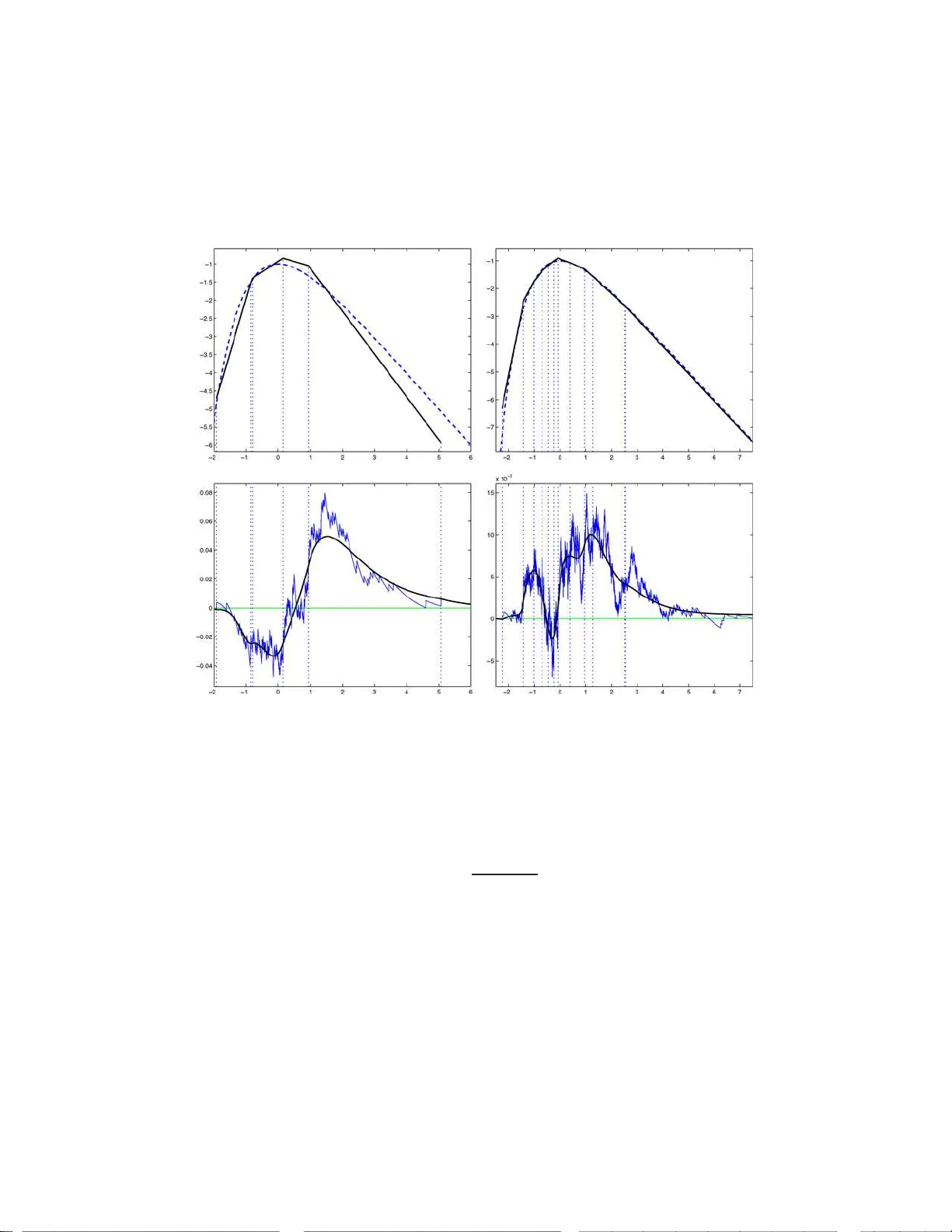
Bernoul li 15 (1), 2009, 40–68 DOI: 10.315 0/08-BEJ 141 Maxim um lik eliho o d estimation of a log-conca v e densit y and its distribution function: Basic prop erties and uniform consistency LUTZ D ¨ UMBGEN 1 and KASP AR R UFIBACH 2 1 Institute of Mathematic al Statistics and A ctuarial Scienc e, University of Bern, Sid lerstr asse 5, CH-3012 Bern, Switzerland. E-mail: duemb gen@stat.unib e. ch 2 Ab teilung Biostatist i k, Institut f ¨ ur Sozial- und Pr¨ aventivme dizin, Universit¨ at Z¨ urich, Hirschen- gr ab en 84, CH-8001 Z ¨ urich, Switzerland. E-mail: kasp ar.rufib ach@ifspm.uzh.ch W e study nonparametric maxim um lik elihoo d estimation of a log-concav e probability den sit y and its distribution and hazard function. Some general prop erties of these estimators are deriv ed from tw o characteri zations. It is sh own that the rate of conve rgence with resp ect t o supremum norm on a compact in terv al for the density and hazard rate estimator is at least (log( n ) /n ) 1 / 3 and typicall y (log ( n ) /n ) 2 / 5 , whereas th e difference b et ween the emp iri cal and estimated distribution function v anishes with rate o p ( n − 1 / 2 ) under certain regularit y assumptions. Keywor ds: adaptivity; brack eting; exp onen tial inequality; gap problem; hazard function; metho d of caricatures; sh ape constraints 1. In tro duction Two common appr oac hes to nonparametric densit y estimation are smo othing metho ds and qualitative constraints. The for mer a pproach includes, among others , kernel densit y estimators, es timators based o n discrete wa velets or o ther series ex pansions and estima - tors ba sed o n roughnes s p enalization. Go o d starting po in ts for the v ast literature in this field are Silv e r man ( 1982 , 1986 ) and Donoho et al. ( 199 6 ). A commo n feature of all of these metho ds is that they in volv e certain tuning pa rameters, for example, the order of a kernel and the bandwidth. A prop er choice of these parameters is far fro m trivial s ince optimal v alues dep end on unkno w n prop erties of the underlying density f . The second approach avoids such problems by imposing qualitative pr operties o n f , for example, monotonicity or co n vexit y o n certain in terv als in the univ ar iate cas e. Such assumptions are often plausible or even justified rigoro usly in sp ecific applications. This is an electronic reprint of the original article published by the ISI/BS in Bernoul li , 2009, V ol. 15, No. 1, 40–68 . This reprint d iffers from the original in pagination and typographic detail. 1350-7265 c  2009 ISI/BS Estimating lo g-c onc ave densities 41 Densit y estimation under s hape cons tr ain ts w a s first co nsidered by Grenander ( 1956 ), who fo und that the nonparametric maxim um lik eliho o d estimator (NPMLE) ˆ f mon n of a non-increas ing densit y function f on [0 , ∞ ) is given by the left deriv ative of the lea st concav e ma joran t of the e mpirical cumulativ e distribution function on [0 , ∞ ). This work was contin ued by Rao ( 1969 ) and Gro eneb o om ( 198 5 , 19 88 ), who established asymptotic distribution theory for n 1 / 3 ( f − ˆ f mon n )( t ) at a fixed point t > 0 under certain regular- it y conditions and analyzed the non-Gaussian limit distribution. F or v ar ious es timation problems in volving monotone functions, the t y pical ra te of convergence is O p ( n − 1 / 3 ) po in twise. The rate of con vergence with resp ect to supremum norm is further deceler- ated b y a factor of log( n ) 1 / 3 (Jonker and v an der V aar t ( 2001 )). F or applications of monotone density estimatio n, cons ult, fo r example, Bar lo w et al. ( 1972 ) or Rober tson et al. ( 198 8 ). Monotone estimation can b e ex tended to cov er unimo dal densities. Remember that a density f on the r eal line is unimo dal if ther e exis ts a num b er M = M ( f ) such that f is non-decreas ing on ( − ∞ , M ] and non-increa sing on [ M , ∞ ). If the tr ue mo de is known a priori, unimo dal density estimation bo ils down to monotone es timation in a stra igh tfor- ward manner, but the s itua tion is different if M is unknown. In that ca se, the likelihoo d is un b ounded, problems being ca used by observ a tio ns to o close to a h y pothetical mo de. Even if the mo de was known, the densit y estimator is inconsisten t at the mode, a phe- nomenon called “spiking”. Several metho ds were pro posed to remedy this problem (see W egman ( 19 70 ), W o odro ofe and Sun ( 1993 ), Meyer and W o odro ofe ( 20 04 ) or Kuliko v and Lo puha ¨ a ( 2006 )), but all of them r e quire additional constraints on f . The combination of s hape constr ain ts and smo othing was a ssessed by Eg germont and La-Riccia ( 2000 ). T o improve the slow rate of conv er gence o f n − 1 / 3 in the space L 1 ( R ) for arbitrar y unimo dal densities, they derived a Grenander -t yp e es timator b y taking the deriv ativ e of the le a st co nc ave ma jora n t of an int egrated k ernel densit y estimator rather than the empir ic a l distribution function dire c tly , yielding a rate of conv er gence o f O p ( n − 2 / 5 ). Estimation of a conv ex decreas ing dens ity on [0 , ∞ ) was pionee r ed by Anevski ( 1994 , 2003 ). The problem arose in a study of migrating birds discussed b y Hamp el ( 1987 ). Gro enebo om et al. ( 2001 ) provide a characterization o f the estimator , as well as con- sistency and limiting b eha vior at a fixed p oin t of positive curv ature of the function to be estimated. They found that the estimator must be piecewise linear with knots be- t ween the obser v atio n points. Under the additional as sumption that the true density f is t wice con tin uously differentiable on [0 , ∞ ), they show that the MLE conv erg es a t rate O p ( n − 2 / 5 ) p oint wise, somewha t better tha n in the mono tone case. Monotonicity and conv exity c o nstrain ts on densities on [0 , ∞ ) hav e b een embedded in to the genera l framework of k –monotone densities by Balab da oui and W ellner ( 2008 ). In a technical rep ort, w e provide a more thoroug h discussio n o f the similarities and differences b et ween k -monotone density estimation and the present w ork (D ¨ um bgen and Rufibach ( 2008 )). In the present paper , we impos e an a lternativ e, a nd quite natura l, shape cons train t on the de ns it y f , namely , log-co nca vity . T ha t means f ( x ) = exp ϕ ( x ) 42 L. D ¨ umb gen and K . Rufib ach for some concav e function ϕ : R → [ −∞ , ∞ ). This class is rather flexible, in that it gen- eralizes many common parametric densities. These include all non-degenerate norma l densities, all Ga mma densities with shap e par ameter ≥ 1 , all W eibull densities with exp onen t ≥ 1 and all b eta dens ities with parameter s ≥ 1. F ur ther examples are the logistic and Gum b el densities. Log-co nca ve densities are of interest in econometrics; see Bagnoli and Berg s trom ( 2005 ) for a summary and further exa mples. Bar low and Proschan ( 1975 ) describ e adv antageous prop erties of log -concav e densities in reliability theory , while Chang and W alther ( 2007 ) use log-co nca ve densities as an ingredient in nonparametric mixture mo dels. In nonparametric Ba yesian analys is , to o, log-concavity is of certa in relev ance (Bro oks ( 1998 )). Note that log-concavit y of a density implies that it is also unimo dal. It will turn out that by imp osing log-c onca v ity , one cir cum ven ts the spiking problem mentioned be fo re, which yields a new approa c h to estimating a unimodal, pos sibly skew e d dens it y . Moreov e r , the log-concav e density estimator is fully automatic, in the sense that there is no need to select any bandwidth, kernel function or other tuning pa rameters. Finally , simulating data from the estimated density is rather easy . All of these prop erties make the new estimator app ealing for use in statistica l applications . Little lar ge sample theory is a v aila ble for lo g-concav e estimators th us far. Sengupta and Paul ( 2005 ) co nsidered testing for log-co nc avity of distribution functions on a com- pact interv al. W alther ( 2002 ) intro duced an extension of log-concavit y in the con text of ce r tain mixture mo dels, but his theo ry do es not co ver asymptotic prop erties of the density estimators themselves. Pal et al. ( 2006 ) proved the log-concave NPMLE to b e consistent, but without ra tes of convergence. Concerning the co mputation of the lo g-concav e NPMLE, W alther ( 2002 ) and Pal et al. ( 2006 ) used a crude version of the iter ativ e c on vex minorant (ICM) algor ithm. A detailed description a nd comparis on of several alg orithms c an b e found in Rufibach ( 2007 ), while D¨ um bg e n et al. ( 2007a ) des c ribe an active set algo rithm, which is similar to the vertex reduction alg orithms pr esen ted by Gro eneb oom et al. ( 2008 ) and s eems to b e the most efficient o ne a t present . The ICM a nd activ e set algor ithms a r e implemented within the R pa c k age "l ogcondens " b y Rufibac h a nd D¨ um bg en ( 2 0 06 ), acc e ssible via "CRAN" . Corresp onding MA TLAB co de is av ailable from the fir st author’s homepage. In Sectio n 2 , w e introduce the log-concave maximum lik eliho od density estimator, dis- cuss its basic prop erties a nd der ive t wo c ha racterizations. In Section 3 , we illustrate this estimator with a r e al data example and explain br iefly ho w to s imulate data from the estimated densit y . Co nsistency of this densit y estimator and the corresp onding estima- tor o f the distribution function a r e treated in Section 4 . It is sho wn that the supremum norm b et ween estimated density , ˆ f n , a nd true density on compact subsets of the interior of { f > 0 } conv erg es to zero at rate O p ((log( n ) /n ) γ ), with γ ∈ [1 / 3 , 2 / 5] depending on f ’s smo othness. In particular, o ur estimator adapts to the unknown smo othness o f f . Consistency o f the density estimato r en tails consis tency o f the distribution function es- timator. In fact, under additiona l regularity conditions on f , the differe nce b et ween the empirical c.d.f. and the estimated c.d.f. is of order o p ( n − 1 / 2 ) on compa ct subsets of the int e rior of { f > 0 } . Estimating lo g-c onc ave densities 43 As a by-product of our estimator, note the following. Log-concavit y of the density function f also implies that the corre s ponding ha zard function h = f / (1 − F ) is non- decreasing (cf. Barlow a nd Proschan ( 1975 )). Hence, our estimator s of f and its c.d.f. F e ntail a consistent and non-decrea sing estimator o f h , as pointed o ut at the end of Section 4 . Some aux iliary results, pro ofs and technical arguments are de fer red to the Appendix . 2. The estimators and their basic prop erties Let X be a random v a r iable with distribution function F and Leb esgue density f ( x ) = exp ϕ ( x ) for some concav e fun ction ϕ : R → [ −∞ , ∞ ). Our goal is to estimate f based on a ran- dom sample of size n > 1 fro m F . Let X 1 < X 2 < · · · < X n be the cor responding order statistics. F or any log -concav e probability density f on R , the normalized lo g-lik e lihoo d function a t f is given by Z log f d F n = Z ϕ d F n , (1) where F n stands for the e mpir ical distributio n function o f the sa mple. In order to r elax the constraint of f being a pro babilit y density and to get a criterio n function to maximize ov er the conv ex set of al l concave functions ϕ , we employ the standar d trick o f adding a Lagra ng e term to ( 1 ), leading to the functional Ψ n ( ϕ ) := Z ϕ d F n − Z exp ϕ ( x ) d x (see Silv erman ( 1982 ), Theorem 3 .1). The nonpar ametric ma xim um likelihoo d estimator of ϕ = log f is the ma x imizer of this functional over all concave functions, ˆ ϕ n := a rg ma x ϕ concav e Ψ n ( ϕ ) and ˆ f n := exp ˆ ϕ n . Existenc e, uniqueness and shap e of ˆ ϕ n . One can easily show tha t Ψ n ( ϕ ) > −∞ if and only if ϕ is rea l-v alue d on [ X 1 , X n ]. The following theorem was proven indep endently by Pal et al. ( 2006 ) and Rufibac h ( 2006 ). It also follows fro m more general considerations in D¨ umbgen et al. ( 2007a ), Section 2. Theorem 2. 1. Th e NPMLE ˆ ϕ n exists and is unique. It is line ar on al l intervals [ X j , X j +1 ] , 1 ≤ j < n . Mor e over, ˆ ϕ n = −∞ on R \ [ X 1 , X n ] . 44 L. D ¨ umb gen and K . Rufib ach Char acterizatio ns and further pr op erties. W e provide t wo characterizatio ns of the es- timators ˆ ϕ n , ˆ f n and the c orresp onding distr ibution function ˆ F n , that is , ˆ F n ( x ) = R x −∞ ˆ f n ( r ) d r . The fir st characterization is in ter ms of ˆ ϕ n and p erturbation functions. Theorem 2. 2. L et e ϕ b e a c onc ave function such that { x : e ϕ ( x ) > −∞} = [ X 1 , X n ] . Then, e ϕ = ˆ ϕ n if and only if Z ∆( x ) d F n ( x ) ≤ Z ∆( x ) exp e ϕ ( x ) d x (2) for any ∆ : R → R such that e ϕ + λ ∆ is c onc ave for some λ > 0 . Plugging suitable p erturbation functions ∆ in Theorem 2.2 yields v aluable info r mation ab out ˆ ϕ n and ˆ F n . F or a firs t illustration, let µ ( G ) and V a r( G ) b e the mean and v ar iance, resp ectiv ely , of a distribution (function) G on the real line with finite second momen t. Setting ∆( x ) := ± x or ∆( x ) := − x 2 in Theorem 2.4 yields the following. Corollary 2.3. µ ( ˆ F n ) = µ ( F n ) and V ar( ˆ F n ) ≤ V ar( F n ) . Our second characterizatio n is in terms of the empirical distr ibutio n function F n and the estimated distribution function ˆ F n . F or a co n tinuous a nd piec ewise linear function h : [ X 1 , X n ] → R , we define the set of its “knots” to b e S n ( h ) := { t ∈ ( X 1 , X n ) : h ′ ( t − ) 6 = h ′ ( t +) } ∪ { X 1 , X n } . Recall that ˆ ϕ n is an example of such a function h with S n ( ˆ ϕ n ) ⊂ { X 1 , X 2 , . . . , X n } . Theorem 2.4 . L et e ϕ b e a c onc ave function which is line ar on al l intervals [ X j , X j +1 ] , 1 ≤ j < n , while e ϕ = −∞ on R \ [ X 1 , X n ] . Defining e F ( x ) := R x −∞ exp e ϕ ( r ) d r , we assume further that e F ( X n ) = 1 . Then, e ϕ = ˆ ϕ n and e F = ˆ F n if, and only if for arbitr ary t ∈ [ X 1 , X n ] , Z t X 1 e F ( r ) d r ≤ Z t X 1 F n ( r ) d r (3) with e quality in the c ase of t ∈ S n ( e ϕ ) . A particular conseq uenc e o f Theorem 2.4 is that the distribution function es timator ˆ F n is very clo se to the empirica l distribution function F n on S n ( ˆ ϕ n ). Corollary 2.5. F n − n − 1 ≤ ˆ F n ≤ F n on S n ( ˆ ϕ n ) . Estimating lo g-c onc ave densities 45 Figure 1. Distribution functions and the pro cess D ( t ) for a Gu mb el sample. Figure 1 illustrates Theor em 2 .4 and Corollar y 2.5 . The upp er plot displa ys F n and ˆ F n for a sa mple of n = 2 5 random num b ers g enerated fr o m a Gum b el distribution with density f ( x ) = e − x exp( − e − x ) o n R . The dotted vertical lines indicate the “kink s” o f ˆ ϕ n , that is, a ll t ∈ S n ( ˆ ϕ n ). Note that ˆ F n and F n are indeed very close on the la tter se t, with equality at the right end-p oin t X n . The lower plo t shows the pr ocess D ( t ) := Z t X 1 ( ˆ F n − F n )( r ) d r for t ∈ [ X 1 , X n ]. As pr edicted by Theorem 2.4 , this pro cess is non-p ositive and equals zero on S n ( ˆ ϕ n ). 3. A d ata example In a rece nt consulting cas e, a compan y a sk ed for Mo n te Carlo expe r imen ts to predict the relia bility of a certain device they pro duce. The relia bilit y dep ended in a certain 46 L. D ¨ umb gen and K . Rufib ach deterministic wa y on five different and indep enden t ra ndom input parameter s . F or each input parameter, a sample was av a ilable and the g oal was to fit a s uitable distributio n to simulate from. Here, we foc us o n just one o f thes e input para meters. A t first, we cons ide r ed tw o standard appro a c hes to estimate the unknown densit y f , namely , (i) fitting a Gaussia n densit y ˆ f par with mean µ ( F n ) and v ariance ˆ σ 2 := n ( n − 1) − 1 V ar( F n ); (ii) the kernel density estimator ˆ f ker ( x ) := Z φ ˆ σ / √ n ( x − y ) d F n ( y ) , where φ σ denotes the density of N (0 , σ 2 ). This very small bandwidth ˆ σ / √ n w as chosen to obtain a density with v a riance ˆ σ 2 and to av oid putting to o m uch weight into the tails. Lo oking at the data, approach (i) is clearly inappropriate b ecause our sample of size n = 787 revealed a skewed and s ignifican tly no n-Gaussian dis tribution. This ca n b e seen in Figure 2 , where the multimodal curve corresp onds to ˆ f ker , while the dashed line depicts ˆ f par . Appro ac h (ii) yielded Mo n te Carlo res ults agre e ing well with measured reliabilities, but the engineers ques tioned the multimodality of ˆ f ker . Cho osing a kernel estimator with larger bandwidth would ov eres timate the v ariance a nd put too m uch weigh t into the tails. Thu s, we agr eed o n a third approach and estimated f b y a slightly smo othed version of ˆ f n , ˆ f ∗ n := Z φ ˆ γ ( x − y ) d ˆ F n ( y ) , with ˆ γ 2 := ˆ σ 2 − V ar( ˆ F n ), so that the v ar ia nce of ˆ f ∗ n coincides with ˆ σ 2 . Since log-concavity is pres e r v ed under conv olutio n (cf. Pr´ ekopa ( 1971 )), ˆ f ∗ n is also log-concave. F or the explicit computation of V ar( ˆ F n ), see D ¨ umbgen et al. ( 2007a ). By smo othing, we also av o id the small disco n tinuities of ˆ f n at X 1 and X n . This density estimator is the skewed unimo dal curve in Figur e 2 . It a lso yielded convincing results in the Monte Carlo sim ulations. Note that b oth estimato rs ˆ f n and ˆ f ∗ n are fully automatic. Moreover, it is very easy to sample from these densities: let S n ( ˆ ϕ n ) consist o f x 0 < x 1 < · · · < x m , and consider the data X i tempo rarily as fixed. No w, (a) g e nerate a random index J ∈ { 1 , 2 , . . . , m } with P ( J = j ) = ˆ F n ( x j ) − ˆ F n ( x j − 1 ); (b) g enerate X := x J − 1 + ( x J − x J − 1 ) ·  log(1 + (e Θ − 1) U ) / Θ , if Θ 6 = 0, U, if Θ = 0, where Θ := ˆ ϕ n ( x J ) − ˆ ϕ n ( x J − 1 ) and U ∼ Unif [0 , 1] ; (c) gener ate X ∗ := X + ˆ γ Z with Z ∼ N (0 , 1) , where J , U a nd Z are indep enden t. Then, X ∼ ˆ f n and X ∗ ∼ ˆ f ∗ n . Estimating lo g-c onc ave densities 47 Figure 2. Three comp et in g d ensit y estimators. 4. Uniform consistency Let us introduce some notation. F or any integer n > 1, we define ρ n := log ( n ) /n and the uniform norm of a function g : I → R on an in ter v al I ⊂ R is denoted b y k g k I ∞ := sup x ∈ I | g ( x ) | . W e say that g b elongs to the H¨ older class H β ,L ( I ) with e x ponent β ∈ [1 , 2 ] and co nstan t L > 0 if for all x, y ∈ I , we hav e | g ( x ) − g ( y ) | ≤ L | x − y | , if β = 1 , | g ′ ( x ) − g ′ ( y ) | ≤ L | x − y | β − 1 , if β > 1 . 48 L. D ¨ u mb gen and K. R ufib ach Uniform c onsistency of ˆ ϕ n . Our main result is the following theor em. Theorem 4.1. Assu me for the lo g-density ϕ = log f that ϕ ∈ H β ,L ( T ) for some exp onent β ∈ [1 , 2] , some c onstant L > 0 and a subinterval T = [ A, B ] of the interior of { f > 0 } . Then, max t ∈ T ( ˆ ϕ n − ϕ )( t ) = O p ( ρ β / (2 β +1) n ) , max t ∈ T ( n,β ) ( ϕ − ˆ ϕ n )( t ) = O p ( ρ β / (2 β +1) n ) , wher e T ( n, β ) := [ A + ρ 1 / (2 β +1) n , B − ρ 1 / (2 β +1) n ] . Note that the previous result remains true when we r e place ˆ ϕ n − ϕ with ˆ f n − f . It is w ell known that the ra tes of convergence in Theore m 4.1 are optimal, ev e n if β w a s known (cf. Khas’minskii ( 1978 )). T hus, o ur estimators adapt to the unknown smo othness of f in the range β ∈ [1 , 2] . Also, note that concavity of ϕ implies that it is Lipschit z-contin uous, that is, b elongs to H 1 ,L ( T ) fo r some L > 0 on any int erv al T = [ A, B ] with A > inf { f > 0 } and B < sup { f > 0 } . Hence, one can easily deduce from Theorem 4.1 that ˆ f n is co nsisten t in L 1 ( R ) and that ˆ F n is uniformly co nsisten t. Corollary 4.2. Z | ˆ f n ( x ) − f ( x ) | d x → p 0 and k ˆ F n − F k R ∞ → p 0 . Distanc e of two c onse cutive knots and uniform c onsistency of ˆ F n . By means of Theorem 4.1 , w e can solve a “gap problem” for lo g-concav e density e stimation. The term “gap problem” was first used by Balabdao ui and W ellner ( 2008 ) to descr ibe the pr oblem of computing the distance b et ween tw o consecutive knots of cer tain estimators. Theorem 4. 3. Supp ose that t he assum ptions of The or em 4.1 hold. Ass ume, further, that ϕ ′ ( x ) − ϕ ′ ( y ) ≥ C ( y − x ) for some c onstant C > 0 and arbi tr ary A ≤ x < y ≤ B , wher e ϕ ′ stands for ϕ ′ ( ·− ) or ϕ ′ ( · +) . Th en, sup x ∈ T min y ∈S n ( ˆ ϕ n ) | x − y | = O p ( ρ β / (4 β +2) n ) . Theorems 4.1 and 4.3 , combined with a result of Stute ( 1 982 ) ab out the modulus of contin uity of empirical pro cesses, yield a ra te of convergence for the maximal difference betw een ˆ F n and F n on co mpact in terv als. Theorem 4.4. Under t he assumptions of The or em 4.3 , max t ∈ T ( n,β ) | ˆ F n ( t ) − F n ( t ) | = O p ( ρ 3 β / (4 β +2) n ) . Estimating lo g-c onc ave densities 49 In p articular, if β > 1 , then max t ∈ T ( n,β ) | ˆ F n ( t ) − F n ( t ) | = o p ( n − 1 / 2 ) . Thu s, under certain regularity conditions, the estimators ˆ F n and F n are asymptoti- cally e quiv alent o n compact sets. Conclusio ns of this type ar e known for the Grena nder estimator (cf. Kiefer a nd W olfo witz ( 1976 )) a nd the least squares estima to r of a con vex density on [0 , ∞ ) (cf. Balab daoui and W ellner ( 2007 )). The r esult of Theor em 4.4 is also related to recent res ults of Gin´ e and Nickl ( 2007 , 2008 ). In the latter pap er, they devise kernel density estimato rs with data-driven band- widths which are also ada ptiv e with resp ect to β in a certain range, while the integrated density estimato r is as ymptotically eq uiv a le nt to F n on the whole real line. Ho wever, if β ≥ 3 / 2 , they m ust use kernel functions o f higher order, tha t is, no lo nger non-negative, and simulating data from the resulting estimated density is not straig h tforward. Example. Let us illustrate Theorems 4.1 and 4.4 with simulated data, again from the Gum b el distribution with ϕ ( x ) = − x − e − x . Here, ϕ ′′ ( x ) = − e − x , so the assumptions o f our theorems are satisfied with β = 2 for any compact interv al T . The upper panels of Figure 3 show the tr ue log-density ϕ (dashed line) and the es timator ˆ ϕ n (line) for samples of s iz e s n = 200 (left) and n = 2000 (right) . The lo wer panels show the corresp onding empirical proces ses n 1 / 2 ( F n − F ) (jagge d curves) and n 1 / 2 ( ˆ F n − F ) (smo oth curves). First, the qualit y of the estimator ˆ ϕ n is quite go o d, even in the tails, and the quality increases with sample size, a s expected. Lo oking at the empirical pro cesses, the similar it y betw een n 1 / 2 ( F n − F ) a nd n 1 / 2 ( ˆ F n − F ) increa s es with sample size, to o, but rather slowly . Also, note that the estimator ˆ F n outp e rforms F n in terms of supremum distance from F , which leads us to the next parag raph. Marshal l’s lemma. In all sim ulatio ns w e looked at, the estimator ˆ F n satisfied the in- equality k ˆ F n − F k R ∞ ≤ k F n − F k R ∞ , (4) provided that f is indeed log- conca ve. Figure 3 sho ws t wo numerical examples of this phenomenon. In view of such examples and Mar s hall’s ( 1970 ) lemma abo ut the Grenander estimator ˆ F mon n , we first tr ied to verify that ( 4 ) is correc t a lmost surely and for any n > 1 . Ho wev er , one ca n constr uct co un terexa mples showing that ( 4 ) may be violated, even if the right-hand side is multiplied with an y fixed constant C > 1 . Nevertheless, our first attempts resulted in a version of Marshall’s lemma for c onvex density estimation; see D¨ umbgen et al. ( 2007 ). F or the pr esen t setting, w e conjecture that ( 4 ) is true with asymptotic probability o ne as n → ∞ , that is, P ( k ˆ F n − F k R ∞ ≤ k F n − F k R ∞ ) → 1 . A monotone hazar d r ate estimator. Estimation of a monotone haz a rd r ate is des cribed, for insta nce, in the bo ok b y Rob e rtson et al. ( 1988 ). They dire c tly solve an isotonic 50 L. D ¨ u mb gen and K. R ufib ach Figure 3. Density functions and empirical processes for Gum b el samples of size n = 200 and n = 2000. estimation problem similar to that for the Grenander density estimator. F or this set- ting, Hall et al. ( 2001 ) a nd Hall and v an Keilego m ( 20 0 5 ) consider metho ds based up o n suitable mo difications of kernel estima to rs. Alterna tiv ely , in our setting, it follows from Lemma A.2 in Section 5 that ˆ h n ( x ) := ˆ f n ( x ) 1 − ˆ F n ( x ) defines a simple plug-in estimator of the hazar d rate on ( −∞ , X n ) which is also no n- decreasing. By virtue of Theorem 4.1 and Corollar y 4.2 , it is uniformly co nsisten t on any compact subinterv al of the interior of { f > 0 } . Theorems 4.1 a nd 4.4 even entail a rate of convergence, as follows. Corollary 4.5. Under t he assu mptions of The or em 4.3 , max t ∈ T ( n,β ) | ˆ h n ( t ) − h ( t ) | = O p ( ρ β / (2 β +1) n ) . Estimating lo g-c onc ave densities 51 5. Outlo ok Starting from the results presented here, Balab daoui et al. ( 2008 ) recently deriv ed the po in twise limiting distr ibutio n of ˆ f n . They also consider ed the limiting distribution of argmax x ∈ R ˆ f n ( x ) as a n estimator of the mo de o f f . E mpirical findings of M ¨ uller and Rufibach ( 2008 ) show that the estimator ˆ f n is even useful for extreme v alue statistics. Log-conc ave densities also have po ten tial as building blo cks in mor e complex models (e.g., r egression o r classifica tion) or when handling censor ed data (cf. D¨ umbgen et al. ( 2007a )). Unfortunately , our pro ofs w ork only for fixed compact interv a ls, w he r eas simulations suggest that the estimators per fo rm well on the who le real line. P resen tly , the author s are working on a differen t approach, where ˆ ϕ n is repr esen ted lo cally as a parametric maximum likelihoo d estimator of a log-linear densit y . Presumably , this will deepen our understanding of the log- conca ve NP MLE’s consis tency prop erties, pa rticularly in the tails. F or instance, w e conjecture th at F n and ˆ F n are asymptotically equiv alent on any int e rv a l T o n whic h ϕ ′ is str ic tly decr easing. App endix: Auxiliary results and pro ofs A.1. Two facts ab out log-conca v e densities The following tw o res ults ab out a log-concave density f = exp ϕ a nd its distribution function F are of indep endent interest. The fir st result entails that the density f has at least s ubexp onen tial tails. Lemma A.1. F or arbitr ary p oints x 1 < x 2 , p f ( x 1 ) f ( x 2 ) ≤ F ( x 2 ) − F ( x 1 ) x 2 − x 1 . Mor e over, for x o ∈ { f > 0 } and any re al x 6 = x o , f ( x ) f ( x o ) ≤         h ( x o , x ) f ( x o ) | x − x o |  2 , exp  1 − f ( x o ) | x − x o | h ( x o , x )  if f ( x o ) | x − x o | ≥ h ( x o , x ) , wher e h ( x o , x ) := F (max( x o , x )) − F (min ( x o , x )) ≤  F ( x o ) , if x < x o , 1 − F ( x o ) , if x > x o . A second well-kno wn r esult (Barlow and P roschan ( 1975 ), Lemma 5.8 ) pro v ides further connections betw een the density f a nd the dis tribution function F . In particular, it en tails that f / ( F (1 − F )) is b ounded awa y from zero o n { x : 0 < F ( x ) < 1 } . 52 L. D ¨ u mb gen and K. R ufib ach Lemma A. 2. The function f /F is non-incr e asing on { x : 0 < F ( x ) ≤ 1 } and the function f / (1 − F ) is non-de cr e asing o n { x : 0 ≤ F ( x ) < 1 } . Pro of of Lemma A.1 . T o prov e the first inequalit y , it suffices to consider the non-trivial case of x 1 , x 2 ∈ { f > 0 } . Concavit y of ϕ then entails that F ( x 2 ) − F ( x 1 ) ≥ Z x 2 x 1 exp  x 2 − t x 2 − x 1 ϕ ( x 1 ) + t − x 1 x 2 − x 1 ϕ ( x 2 )  d t = ( x 2 − x 1 ) Z 1 0 exp((1 − u ) ϕ ( x 1 ) + uϕ ( x 2 )) d u ≥ ( x 2 − x 1 ) exp  Z 1 0 ((1 − u ) ϕ ( x 1 ) + uϕ ( x 2 )) d u  = ( x 2 − x 1 ) exp( ϕ ( x 1 ) / 2 + ϕ ( x 2 ) / 2) = ( x 2 − x 1 ) p f ( x 1 ) f ( x 2 ) , where the seco nd inequality follows fro m Jensen’s inequality . W e prov e the second asserted inequality only for x > x o , that is, h ( x o , x ) = F ( x ) − F ( x o ), the other ca se b eing handled analogo usly . The first part entails that f ( x ) f ( x o ) ≤  h ( x o , x ) f ( x o )( x − x o )  2 , and the r igh t-ha nd side is not greater than o ne if f ( x o )( x − x o ) ≥ h ( x o , x ). I n the latter case, reca ll that h ( x o , x ) ≥ ( x − x o ) Z 1 0 exp((1 − u ) ϕ ( x o ) + uϕ ( x )) d u = f ( x o )( x − x o ) J ( ϕ ( x ) − ϕ ( x o )) with ϕ ( x ) − ϕ ( x o ) ≤ 0, where J ( y ) := R 1 0 exp( uy ) d u . Elementary calculations show that J ( − r ) = (1 − e − r ) /r ≥ 1 / (1 + r ) for arbitrar y r > 0 . Thu s, h ( x o , x ) ≥ f ( x o )( x − x o ) 1 + ϕ ( x o ) − ϕ ( x ) , which is eq uiv a le nt to f ( x ) /f ( x o ) ≤ exp(1 − f ( x o )( x − x o ) /h ( x o , x )).  A.2. Pr oofs of the characterizations Pro of of Theorem 2.2 . In view of Theorem 2.1 , w e may restrict our atten tion to concav e and re a l-v a lued functions ϕ on [ X 1 , X n ] and set ϕ := −∞ on R \ [ X 1 , X n ]. The set C n of all s uc h functions is a conv ex cone a nd for an y function ∆ : R → R and t > 0, concavit y o f ϕ + t ∆ o n R is equiv alent to its co nca vity on [ X 1 , X n ]. Estimating lo g-c onc ave densities 53 One can easily verify that Ψ n is a co nca ve and real-v alue d functional on C n . Hence, as well k no wn from co n vex analysis, a function e ϕ ∈ C n maximizes Ψ n if a nd only if lim t ↓ 0 Ψ n ( e ϕ + t ( ϕ − e ϕ )) − Ψ n ( e ϕ ) t ≤ 0 for a ll ϕ ∈ C n . But, this is equiv alent to the re quiremen t that lim t ↓ 0 Ψ n ( e ϕ + t ∆) − Ψ n ( e ϕ ) t ≤ 0 for any function ∆ : R → R s uc h that e ϕ + λ ∆ is concave for so me λ > 0. The ass ertion of the theo rem now follows fr o m lim t ↓ 0 Ψ n ( e ϕ + t ∆) − Ψ n ( e ϕ ) t = Z ∆ d F n − Z ∆( x ) exp e ϕ ( x ) d x.  Pro of of Theorem 2.4 . W e start with a general observ ation. Let G be some distribution (function) with supp ort [ X 1 , X n ] and let ∆ : [ X 1 , X n ] → R b e absolutely contin uous with L 1 -deriv ative ∆ ′ . It then follows from F ubini’s theorem that Z ∆ d G = ∆( X n ) − Z X n X 1 ∆ ′ ( r ) G ( r ) d r. (A.1) Now, suppose that e ϕ = ˆ ϕ n and let t ∈ ( X 1 , X n ]. Let ∆ be absolutely co n tinuous on [ X 1 , X n ] with L 1 –deriv ative ∆ ′ ( r ) = 1 { r ≤ t } a nd ar bitrary v alue o f ∆( X n ). Clear ly , e ϕ + ∆ is concav e, w he nc e ( 2 ) and ( A.1 ) entail that ∆( X n ) − Z t X 1 F n ( r ) d r ≤ ∆( X n ) − Z t X 1 e F ( r ) d r, which is equiv alent to ineq ualit y ( 3 ). In the ca se of t ∈ S n ( e ϕ ) \ { X 1 } , let ∆ ′ ( r ) = − 1 { r ≤ t } . Then, e ϕ + λ ∆ is concav e for so me λ > 0 so that ∆( X n ) + Z t X 1 F n ( r ) d r ≤ ∆( X n ) + Z t X 1 e F ( r ) d r, which y ie lds equality in ( 3 ). Now, supp ose tha t e ϕ s atisfies inequality ( 3 ) for all t with equa lit y if t ∈ S n ( e ϕ ). In view of Theorem 2.1 and the proo f of Theor em 2 .2 , it suffices to sho w that ( 2 ) holds fo r any function ∆ defined on [ X 1 , X n ] which is linear o n each interv al [ X j , X j +1 ], 1 ≤ j < n , while e ϕ + λ ∆ is concave for s ome λ > 0. The latter requirement is equiv alent to ∆ b eing concav e betw ee n t wo consecutive knots of e ϕ . Elemen tar y co nsiderations sho w that the L 1 -deriv ative of s uch a function ∆ may b e written as ∆ ′ ( r ) = n X j =2 β j 1 { r ≤ X j } , 54 L. D ¨ u mb gen and K. R ufib ach with r eal n umber s β 2 , . . . , β n such that β j ≥ 0 if X j / ∈ S n ( e ϕ ) . Consequently , it follows fr om ( A.1 ) and our a s sumptions on e ϕ that Z ∆ d F n = ∆( X n ) − n X j =2 β j Z X j X 1 F n ( r ) d r ≤ ∆( X n ) − n X j =2 β j Z X j X 1 e F ( r ) d r = Z ∆ d e F .  Pro of of Corollary 2.5 . F or t ∈ S n ( ˆ ϕ n ) and s < t < u , it follows fro m Theor e m 2.4 that 1 u − t Z u t ˆ F n ( r ) d r ≤ 1 u − t Z t s F n ( r ) d r and 1 t − s Z t s ˆ F n ( r ) d r ≥ 1 t − s Z t s F n ( r ) d r . Letting u ↓ t and s ↑ t yields ˆ F n ( t ) ≤ F n ( t ) and ˆ F n ( t ) ≥ F n ( t − ) = F n ( t ) − n − 1 .  A.3. Pr oof of ˆ ϕ n ’s consistency Our pro of of Theorem 4.1 inv olves a refinement and mo dification of metho ds introduced by D ¨ umbgen et al. ( 2004 ). A first key ingredient is an inequality for concav e functions due to D ¨ um bg en ( 1998 ) (se e a lso D¨ umbgen et al. ( 2004 ) o r Rufibach ( 2006 )). Lemma A.3. F or any β ∈ [1 , 2] and L > 0 , ther e exists a c onstant K = K ( β , L ) ∈ (0 , 1] with the fo l lowing pr op erty. Supp ose that g and ˆ g ar e c onc ave and r e al-value d fun ctions on a c omp act int erva l T = [ A, B ] , wher e g ∈ H β ,L ( T ) . L et ǫ > 0 and 0 < δ ≤ K min { B − A, ǫ 1 /β } . The n sup t ∈ T ( ˆ g − g ) ≥ ǫ or sup t ∈ [ A + δ,B − δ ] ( g − ˆ g ) ≥ ǫ implies that inf t ∈ [ c,c + δ ] ( ˆ g − g )( t ) ≥ ǫ/ 4 or inf t ∈ [ c,c + δ ] ( g − ˆ g )( t ) ≥ ǫ/ 4 for some c ∈ [ A, B − δ ] . Estimating lo g-c onc ave densities 55 Starting from this lemma, let us first sketch the idea of our pro of of Theorem 4.1 . Suppo se we had a family D of mea surable functions ∆ with finite seminorm σ (∆) :=  Z ∆ 2 d F  1 / 2 , such that sup ∆ ∈D | R ∆ d( F n − F ) | σ (∆) ρ 1 / 2 n ≤ C (A.2) with asymptotic probabilit y one, where C > 0 is some constan t. If, in addition, ϕ − ˆ ϕ n ∈ D and ϕ − ˆ ϕ n ≤ C with asy mptotic probability o ne, then we could conclude that     Z ( ϕ − ˆ ϕ n ) d( F n − F )     ≤ C σ ( ϕ − ˆ ϕ n ) ρ 1 / 2 n , while Theor em 2.2 , applied to ∆ := ϕ − ˆ ϕ n , en ta ils that Z ( ϕ − ˆ ϕ n ) d( F n − F ) ≤ Z ( ϕ − ˆ ϕ n ) d( ˆ F − F ) = − Z ∆(1 − exp( − ∆)) d F ≤ − (1 + C ) − 1 Z ∆ 2 d F = − (1 + C ) − 1 σ ( ϕ − ˆ ϕ n ) 2 bec ause y (1 − exp( − y )) ≥ (1 + y + ) − 1 y 2 for all real y , where y + := max( y , 0). Hence, with asymptotic probability o ne, σ ( ϕ − ˆ ϕ n ) 2 ≤ C 2 (1 + C ) 2 ρ n . Now, supp ose that | ϕ − ˆ ϕ n | ≥ ǫ n on a subint erv al of T = [ A, B ] of length ǫ 1 /β n , where ( ǫ n ) n is a fixed sequence of num b e rs ǫ n > 0 tending to ze r o. Then, σ ( ϕ − ˆ ϕ n ) 2 ≥ ǫ (2 β +1) /β n min T ( f ), so that ǫ n ≤ e C ρ 2 β / (2 β +1) n with e C = ( C 2 (1 + C ) 2 / min T ( f )) β / (2 β +1) . The previous cons iderations will be mo dified in t wo asp ects to get a rigorous pr oof of Theorem 4.1 . F or tec hnical reasons, w e m us t replace the denominator σ (∆) ρ 1 / 2 n of inequality ( A.2 ) with σ (∆) ρ 1 / 2 n + W (∆) ρ 2 / 3 n , where W (∆) := sup x ∈ R | ∆( x ) | max(1 , | ϕ ( x ) | ) . 56 L. D ¨ u mb gen and K. R ufib ach This is necessa ry to dea l with functions ∆ with small v alues of F ( { ∆ 6 = 0 } ). Moreov er , we shall w o rk with simple “ca ricatures” of ϕ − ˆ ϕ n , namely , functions which are piecewise linear with at most three knots. Throughout this section, piecewise linearity do es not necessarily imply con tinuit y . A function b eing piece w is e linear with a t mo st m k nots means that the rea l line may be partitioned into m + 1 non-degenera te interv als on e ac h of which the function is linear. Then, the m real b oundary p oin ts of these interv als ar e the k nots. The next lemma extends inequality ( 2 ) to certain piec e wise linear functions. Lemma A.4. L et ∆ : R → R b e pie c ewise line ar such that e ach knot q of ∆ satisfies one of the f ol lowing two pr op erties: q ∈ S n ( ˆ ϕ n ) and ∆( q ) = lim inf x → q ∆( x ); (A.3) ∆( q ) = lim r → q ∆( r ) and ∆ ′ ( q − ) ≥ ∆ ′ ( q +) . (A.4) Then, Z ∆ d F n ≤ Z ∆ d ˆ F n . (A.5) W e can now sp ecify the “c aricatures” men tioned ab ov e. Lemma A.5. L et T = [ A, B ] b e a fi xe d subinterval of the interior of { f > 0 } . L et ϕ − ˆ ϕ n ≥ ǫ or ˆ ϕ n − ϕ ≥ ǫ on some interval [ c , c + δ ] ⊂ T with lengt h δ > 0 and supp ose that X 1 < c and X n > c + δ . Ther e then exists a pie c ewise line ar function ∆ with at most thr e e knots, e ach of which satisfies c ondition ( A.3 ) or ( A.4 ) , and a p ositive c onstant K ′ = K ′ ( f , T ) such that | ϕ − ˆ ϕ n | ≥ ǫ | ∆ | , (A.6) ∆( ϕ − ˆ ϕ n ) ≥ 0 , (A.7) ∆ ≤ 1 , (A.8) Z c + δ c ∆ 2 ( x ) d x ≥ δ / 3 , (A.9) W (∆) ≤ K ′ δ − 1 / 2 σ (∆) . (A.10) Our last ingr edien t is a surr ogate for ( A.2 ). Lemma A.6. L et D m b e the family o f a l l pi e c ewise line ar functions on R with at most m knots. Ther e exists a c onst ant K ′′ = K ′′ ( f ) such that sup m ≥ 1 , ∆ ∈D m | R ∆ d( F n − F ) | σ (∆) m 1 / 2 ρ 1 / 2 n + W (∆) mρ 2 / 3 n ≤ K ′′ , Estimating lo g-c onc ave densities 57 with pr ob ability tending to o ne as n → ∞ . Before we verify all of these auxiliary r esults, let us pr oceed with the main pro of. Pro of of Theorem 4.1 . Suppo se that sup t ∈ T ( ˆ ϕ n − ϕ )( t ) ≥ C ǫ n or sup t ∈ [ A + δ n ,B − δ n ] ( ϕ − ˆ ϕ n )( t ) ≥ C ǫ n for some constant C > 0, where ǫ n := ρ β / (2 β +1) n and δ n := ρ 1 / (2 β +1) n = ǫ 1 /β n . It follows from Lemma A.3 with ǫ := C ǫ n that in the case of C ≥ K − β and for sufficiently larg e n , there is a (random) in terv al [ c n , c n + δ n ] ⊂ T on which either ˆ ϕ n − ϕ ≥ ( C / 4) ǫ n or ϕ − ˆ ϕ n ≥ ( C / 4) ǫ n . But, then, there is a (random) function ∆ n ∈ D 3 fulfilling the co nditions stated in Lemma A.5 . F or this ∆ n , it follows fro m ( A.5 ) that Z R ∆ n d( F − F n ) ≥ Z R ∆ n d( F − ˆ F n ) = Z R ∆ n (1 − ex p[ − ( ϕ − ˆ ϕ n )]) d F . (A.11) With e ∆ n := ( C / 4) ǫ n ∆ n , it follows from ( A.6 – A.7 ) that the righ t-ha nd side of ( A.11 ) is not smalle r than (4 /C ) ǫ − 1 n Z e ∆ n (1 − ex p( − e ∆ n )) d F ≥ (4 /C ) ǫ − 1 n 1 + ( C / 4) ǫ n σ ( e ∆ n ) 2 = ( C / 4) ǫ n 1 + o (1) σ (∆ n ) 2 bec ause e ∆ n ≤ ( C / 4) ǫ n , by ( A.8 ). On the o ther hand, according to Lemma A.6 , we may assume that Z R ∆ n d( F − F n ) ≤ K ′′ (3 1 / 2 σ (∆ n ) ρ 1 / 2 n + 3 W (∆ n ) ρ 2 / 3 n ) ≤ K ′′ (3 1 / 2 ρ 1 / 2 n + 3 K ′ δ − 1 / 2 n ρ 2 / 3 n ) σ (∆ n ) (b y ( A.10 )) ≤ K ′′ (3 1 / 2 ρ 1 / 2 n + 3 K ′ ρ 2 / 3 − 1 / (4 β +2) n ) σ (∆ n ) ≤ Gρ 1 / 2 n σ (∆ n ) for s ome consta n t G = G ( β , L, f , T ) b ecause 2 / 3 − 1 / (4 β + 2) ≥ 2 / 3 − 1 / 6 = 1 / 2. Conse- quently , C 2 ≤ 16 G 2 (1 + o (1)) ǫ − 2 n ρ n σ (∆ n ) 2 = 16 G 2 (1 + o (1)) δ − 1 n σ (∆ n ) 2 ≤ 48 G 2 (1 + o (1)) min T ( f ) , where the las t inequality fo llo ws from ( A.9 ).  58 L. D ¨ u mb gen and K. R ufib ach Pro of of Lemma A.4 . There is a seq uence of contin uo us, piecewise linear functions ∆ k conv erg ing p o in twise isotonically to ∆ a s k → ∞ suc h that a ny knot q of ∆ k either belo ngs to S n ( ˆ ϕ n ) o r ∆ ′ k ( q − ) > ∆ ′ k ( q +). Thus, ˆ ϕ n + λ ∆ k is concave for sufficiently sma ll λ > 0. Consequently , since ∆ 1 ≤ ∆ k ≤ ∆ for all k , it follows from do minated conv ergenc e and ( 2 ) that Z ∆ d F n = lim k →∞ Z ∆ k d F n ≤ lim k →∞ Z ∆ k d ˆ F n = Z ∆ d ˆ F n .  Pro of of Lemma A.5 . The crucial point in a ll the ca ses w e must disting uish is to construct a ∆ ∈ D 3 satisfying the assumptions of Lemma A.4 and ( A.6 – A.9 ). Rec all that ˆ ϕ n is piecewis e linear. Case 1a : ˆ ϕ n − ϕ ≥ ǫ on [ c, c + δ ] and S n ( ˆ ϕ n ) ∩ ( c, c + δ ) 6 = ∅ . Here , w e c ho ose a contin uous function ∆ ∈ D 3 with knots c , c + δ a nd x o ∈ S n ( ˆ ϕ n ) ∩ ( c, c + δ ), where ∆ := 0 on ( − ∞ , c ] ∪ [ c + δ, ∞ ) and ∆( x o ) := − 1. Here, the assumptions of Le mma A.4 and requirements ( A.6 – A.9 ) are ea sily verified. Case 1b : ˆ ϕ n − ϕ ≥ ǫ on [ c, c + δ ] and S n ( ˆ ϕ n ) ∩ ( c, c + δ ) = ∅ . Let [ c o , d o ] ⊃ [ c, c + δ ] be the maximal interv al on which ϕ − ˆ ϕ n is concav e. There then exists a linear function e ∆ such that e ∆ ≥ ϕ − ˆ ϕ n on [ c o , d o ] and e ∆ ≤ − ǫ on [ c, c + δ ]. Next, let ( c 1 , d 1 ) := { e ∆ < 0 } ∩ ( c o , d o ). W e now define ∆ ∈ D 2 via ∆( x ) :=  0 , if x ∈ ( −∞ , c 1 ) ∪ ( d 1 , ∞ ), e ∆ /ǫ, if x ∈ [ c 1 , d 1 ]. Again, the assumptions of Le mma A.4 a nd requirements ( A.6 – A.9 ) are easily verified; this time, we even kno w that ∆ ≤ − 1 on [ c, c + δ ], whe nc e R c + δ c ∆( x ) 2 d x ≥ δ . Figure 4 illustrates this c o nstruction. Case 2 : ϕ − ˆ ϕ n ≥ ǫ o n [ c, c + δ ] . Let [ c o , c ] and [ c + δ, d o ] be maximal in terv als on which ˆ ϕ n is linear . W e then define ∆( x ) :=    0 , if x ∈ ( −∞ , c o ) ∪ ( d o , ∞ ), 1 + β 1 ( x − x o ) , if x ∈ [ c o , x o ], 1 + β 2 ( x − x o ) , if x ∈ [ x o , d o ], where x o := c + δ/ 2 and β 1 ≥ 0 is chosen suc h that either ∆( c o ) = 0 and ( ϕ − ˆ ϕ n )( c o ) ≥ 0 , or ( ϕ − ˆ ϕ n )( c o ) < 0 and sign(∆) = sign( ϕ − ˆ ϕ n ) on [ c o , x o ] . Analogously , β 2 ≤ 0 is chosen s uc h that ∆( d o ) = 0 and ( ϕ − ˆ ϕ n )( d o ) ≥ 0 , or ( ϕ − ˆ ϕ n )( d o ) < 0 and sign(∆) = sign( ϕ − ˆ ϕ n ) on [ x o , d o ] . Again, the assumptions of Le mma A.4 a nd requirements ( A.6 – A.9 ) are easily verified. Figure 5 depicts an example. Estimating lo g-c onc ave densities 59 Figure 4. The p erturbation function ∆ in Case 1b. It rema ins to verify requir e men t ( A.10 ) for our particular functions ∆. Note that by o ur assumption on T = [ A, B ] , there exist num b ers τ , C o > 0 suc h that f ≥ C o on T o := [ A − τ , B + τ ] . In Cas e 1a, W (∆) ≤ k ∆ k R ∞ = 1 , whereas σ (∆) 2 ≥ C o R c + δ c ∆( x ) 2 d x = C o δ 2 / 3. Hence, ( A.10 ) is sa tisfied if K ′ ≥ (3 /C o ) 1 / 2 . F or Cases 1b and 2, w e start with a more gener al consider ation. Let h ( x ) := 1 { x ∈ Q } ( α + γ x ) for real num b ers α, γ a nd a non-degene r ate interv a l Q co n taining so me p o in t in ( c, c + δ ) . Let Q ∩ T o hav e end-p oin ts x o < y o . Elementary cons iderations then r ev eal that σ ( h ) 2 ≥ C o Z y o x o ( α + γ x ) 2 d x ≥ C o 4 ( y o − x o )( k h k T o ∞ ) 2 . W e now deduce an upp er b ound for W ( h ) / k h k T o ∞ . If Q ⊂ T o or γ = 0 , then W ( h ) / k h k T o ∞ ≤ 1. Now, suppo se that γ 6 = 0 and Q 6⊂ T o . Then, x o , y o ∈ T o satisfy y o − x o ≥ τ and, without loss of gener alit y , le t γ = − 1 . Now, k h k T o ∞ = max( | α − x o | , | α − y o | ) = ( y o − x o ) / 2 + | α − ( x o + y o ) / 2 | ≥ τ / 2 + | α − ( x o + y o ) / 2 | . 60 L. D ¨ u mb gen and K. R ufib ach Figure 5. The p erturbation function ∆ in Case 2. On the other hand, since ϕ ( x ) ≤ a o − b o | x | for c ertain constants a o , b o > 0, W ( h ) ≤ sup x ∈ R | α − x | max(1 , b o | x | − a o ) ≤ sup x ∈ R | α | + | x | max(1 , b o | x | − a o ) = | α | + ( a o + 1) /b o ≤ | α − ( x o + y o ) / 2 | + ( | A | + | B | + τ ) / 2 + ( a o + 1) /b o . This entails that W ( h ) k h k T o ∞ ≤ C ∗ := ( | A | + | B | + τ ) / 2 + ( a o + 1) /b o τ / 2 . In Case 1b, our function ∆ is of the s ame type as h ab o ve and y o − x o ≥ δ . Thus, W (∆) ≤ C ∗ k h k T o ∞ ≤ 2 C ∗ C − 1 / 2 o δ − 1 / 2 σ (∆) . Estimating lo g-c onc ave densities 61 In Case 2, ∆ may b e written as h 1 + h 2 , with tw o functions h 1 and h 2 of the same t yp e as h above having disjoint supp ort a nd both sa tis fying y o − x o ≥ δ / 2. Thus, W (∆) = max( W ( h 1 ) , W ( h 2 )) ≤ 2 3 / 2 C ∗ C − 1 / 2 o δ − 1 / 2 max( σ ( h 1 ) , σ ( h 2 )) ≤ 2 3 / 2 C ∗ C − 1 / 2 o δ − 1 / 2 σ (∆) .  T o prov e Lemma A.6 , we need a simple exp onen tial inequa lit y . Lemma A.7. L et Y b e a r andom variable such that E ( Y ) = 0 , E ( Y 2 ) = σ 2 and C := E exp( | Y | ) < ∞ . Then, for arbitr ary t ∈ R , E exp( tY ) ≤ 1 + σ 2 t 2 2 + C | t | 3 (1 − | t | ) + . Pro of. E exp( tY ) = ∞ X k =0 t k k ! E ( Y k ) ≤ 1 + σ 2 t 2 2 + ∞ X k =3 | t | k k ! E ( | Y | k ) . F or any y ≥ 0 a nd in tegers k ≥ 3, y k e − y ≤ k k e − k . Thus, E ( | Y | k ) ≤ E exp( | Y | ) k k e − k = C k k e − k . Since k k e − k ≤ k !, which ca n be verified ea sily via induction o n k , ∞ X k =3 | t | k k ! E ( | Y | k ) ≤ C ∞ X k =3 | t | k = C | t | 3 (1 − | t | ) + .  Lemma A.7 en tails the following result for finite families of functions. Lemma A.8. L et H n b e a finite family of functions h with 0 < W ( h ) < ∞ such that # H n = O ( n p ) fo r some p > 0 . Then, for sufficiently la r ge D , lim n →∞ P  max h ∈H n | R h d( F n − F ) | σ ( h ) ρ 1 / 2 n + W ( h ) ρ 2 / 3 n ≥ D  = 0 . Pro of. Since W ( ch ) = cW ( h ) and σ ( ch ) = cσ ( h ) for any h ∈ H n and arbitrar y constants c > 0, we may assume, without loss of generality , that W ( h ) = 1 for all h ∈ H n . Let X be a random v ariable with log -densit y ϕ . Since lim sup | x |→∞ ϕ ( x ) | x | < 0 by Lemma A.1 , the exp ectation of exp( t o w ( X )) is finit e for any fixed t o ∈ (0 , 1) , wher e w ( x ) := max(1 , | ϕ ( x ) | ). Hence, E exp( t o | h ( X ) − E h ( X ) | ) ≤ C o := exp( t o E w ( X )) E exp( t o w ( X )) < ∞ . 62 L. D ¨ u mb gen and K. R ufib ach Lemma A.7 , applied to Y := t o ( h ( X ) − E h ( X )) , implies that E exp[ t ( h ( X ) − E h ( X ))] = E (( t/t o ) Y ) ≤ 1 + σ ( h ) 2 t 2 2 + C 1 | t | 3 (1 − C 2 | t | ) + for arbitrar y h ∈ H n , t ∈ R and constants C 1 , C 2 depe nding on t o and C o . Conse q uen tly , E exp  t Z h d( F n − F )  = E exp ( t/n ) n X i =1 ( h ( X i ) − E h ( X )) ! = ( E exp(( t/n )( h ( X ) − E h ( X )) )) n ≤  1 + σ ( h ) 2 t 2 2 n 2 + C 1 | t | 3 n 3 (1 − C 2 | t | /n ) +  n ≤ exp  σ ( h ) 2 t 2 2 n + C 1 | t | 3 n 2 (1 − C 2 | t | /n ) +  . It now follows from Marko v’s inequality that P      Z h d( F n − F )     ≥ η  ≤ 2 e x p  σ ( h ) 2 t 2 2 n + C 1 t 3 n 2 (1 − C 2 t/n ) + − tη  (A.12) for a rbitrary t, η > 0 . Sp ecifically , let η = D ( σ ( h ) ρ 1 / 2 n + ρ 2 / 3 n ) a nd set t := nρ 1 / 2 n σ ( h ) + ρ 1 / 6 n ≤ nρ 1 / 3 n = o ( n ) . Then, the b ound ( A.12 ) is not greater than 2 exp  σ ( h ) 2 log n 2( σ ( h ) + ρ 1 / 6 n ) 2 + C 1 ρ 1 / 2 n log n ( σ ( h ) + ρ 1 / 6 n ) 3 (1 − C 2 ρ 1 / 3 n ) + − D lo g n  ≤ 2 e x p  1 2 + C 1 (1 − C 2 ρ 1 / 3 n ) + − D  log n  = 2 e x p (( O (1) − D ) log n ) . Consequently , for sufficiently large D > 0, P  max h ∈H n | R h d( F n − F ) | σ ( h ) ρ 1 / 2 n + W ( h ) ρ 2 / 3 n ≥ D  ≤ # H n 2 exp(( O (1) − D ) log n ) = O (1) exp( ( O (1) + p − D ) log n ) → 0 .  Pro of of Lemm a A.6 . Let H be the family o f all functions h of the form h ( x ) = 1 { x ∈ Q } ( c + d x ) , Estimating lo g-c onc ave densities 63 with any interv a l Q ⊂ R and real constants c , d such that h is non-neg a tiv e. Supp ose that there ex is ts a constant C = C ( f ) such that P  sup h ∈H | R h d( F n − F ) | σ ( h ) ρ 1 / 2 n + W ( h ) ρ 2 / 3 n ≤ C  → 1 . (A.13) F or any m ∈ N , an arbitrar y function ∆ ∈ D m may be written as ∆ = M X i =1 h i with M = 2 m + 2 functions h i ∈ H having pair wise dis join t supp orts. Consequently , σ (∆) = M X i =1 σ ( h i ) 2 ! 1 / 2 ≥ M − 1 / 2 M X i =1 σ ( h i ) , by the Cauchy–Sc hw ar z inequality , while W (∆) = max i =1 ,...,M W ( h i ) ≥ M − 1 M X i =1 W ( h i ) . Consequently , ( A.13 ) entails that     Z ∆ d( F n − F )     ≤ M X i =1     Z h i d( F n − F )     ≤ C M X i =1 σ ( h i ) ρ 1 / 2 n + M X i =1 W ( h i ) ρ 2 / 3 n ! ≤ 4 C ( σ (∆) m 1 / 2 ρ 1 / 2 n + W (∆) mρ 2 / 3 n ) uniformly in m ∈ N and ∆ ∈ D m , with pro babilit y tending to one as n → ∞ . It remains to verify ( A.13 ). T o this end, we us e a br ac keting ar gumen t. With the weigh t function w ( x ) = ma x( 1 , | ϕ ( x ) | ), let −∞ = t n, 0 < t n, 1 < · · · < t n,N ( n ) = ∞ s uc h that for I n,j := ( t n,j − 1 , t n,j ], (2 n ) − 1 ≤ Z I n,j w ( x ) 2 f ( x ) d x ≤ n − 1 for 1 ≤ j ≤ N ( n ) , with equality if j < N ( n ). Since 1 ≤ R exp( t o w ( x )) f ( x ) d x < ∞ , such a pa rtition exists with N ( n ) = O ( n ) . F or any h ∈ H , we define functions h n,ℓ , h n,u as follows. Let { j, . . . , k } be the set of all indices i ∈ { 1 , . . . , N ( n ) } such that { h > 0 } ∩ I n,i 6 = ∅ . W e then define h n,ℓ ( x ) := 1 { t n,j j } W ( h ) g n,k , with g n,i ( x ) := 1 { x ∈ I n,i } w ( x ) . Consequent ly , all functions in H n are linear com binations with n on-ne gative co efficien ts of at most four functions in the finite family G n := { g n,i : 1 ≤ i ≤ N ( n ) } ∪ { g (1) n,j,k , g (2) n,j,k : 1 ≤ j < k ≤ N ( n ) } . Since G n contains O ( n 2 ) functions, it follows from Lemma A.8 that for s o me constant D > 0,     Z g d( F n − F )     ≤ D ( σ ( g ) ρ 1 / 2 n + W ( g ) ρ 2 / 3 n ) for all g ∈ G n with asymptotic proba bilit y one. The ass ertion ab out H n now follows from the basic o bserv ation that for h = P 4 i =1 α i g i with non-negative functions g i and co efficien ts α i ≥ 0, σ ( h ) ≥ 4 X i =1 α 2 i σ ( g i ) 2 ! 1 / 2 ≥ 2 − 1 4 X i =1 α i σ ( g i ) , W ( h ) ≥ ma x i =1 ,..., 4 α i W ( g i ) ≥ 4 − 1 4 X i =1 α i W ( g i ) .  A.4. Pr oofs for the gap problem and of ˆ F n ’s consistency Pro of of Theorem 4.3 . Suppo se that ˆ ϕ n is linear on an interv a l [ a, b ]. Then, for x ∈ [ a, b ] and λ x := ( x − a ) / ( b − a ) ∈ [0 , 1] , ϕ ( x ) − (1 − λ x ) ϕ ( a ) − λ x ϕ ( b ) = (1 − λ x )( ϕ ( x ) − ϕ ( a )) − λ x ( ϕ ( b ) − ϕ ( x )) = (1 − λ x ) Z x a ϕ ′ ( t ) d t − λ x Z b x ϕ ′ ( t ) d t = (1 − λ x ) Z x a ( ϕ ′ ( t ) − ϕ ′ ( x )) d t + λ x Z b x ( ϕ ′ ( x ) − ϕ ′ ( t )) d t ≥ C (1 − λ x ) Z x a ( x − t ) d t + C λ x Z b x ( t − x ) d t = C ( b − a ) 2 λ x (1 − λ x ) / 2 = C ( b − a ) 2 / 8 if x = x o := ( a + b ) / 2 . 66 L. D ¨ u mb gen and K. R ufib ach This en ta ils that sup [ a,b ] | ˆ ϕ n − ϕ | ≥ C ( b − a ) 2 / 16 . F or if ˆ ϕ n < ϕ + C ( b − a ) 2 / 16 o n { a, b } , then ϕ ( x o ) − ˆ ϕ n ( x o ) = ϕ ( x o ) − ( ˆ ϕ n ( a ) + ˆ ϕ n ( b )) / 2 > ϕ ( x o ) − ( ϕ ( a ) + ϕ ( b )) / 2 − C ( b − a ) 2 / 16 ≥ C ( b − a ) 2 / 8 − C ( b − a ) 2 / 16 = C ( b − a ) 2 / 16 . Consequently , if | ˆ ϕ n − ϕ | ≤ D n ρ β / (2 β +1) n on T n := [ A + ρ 1 / (2 β +1) n , B − ρ 1 / (2 β +1) n ] with D n = O p (1), then the longest subinterv al of T n containing no p oin ts from S n has leng th at most 4 D 1 / 2 n C − 1 / 2 ρ β / (4 β +2) n . Since T n and T = [ A, B ] differ by tw o interv als of leng th ρ 1 / (2 β +1) n = O ( ρ β / (4 β +2) n ), these considera tio ns yield the assertion abo ut S n ( ˆ ϕ n ).  Pro of of T heorem 4.4 . Let δ n := ρ 1 / (2 β +1) n and r n := D ρ β / (4 β +2) n = D δ 1 / 2 n for some constant D > 0. Since r n → 0 but nr n → ∞ , it follows from b oundedness of f a nd a theorem of Stute (1982) ab out the modulus of contin uity of univ ariate empirica l pro cesses that ω n := sup x,y ∈ R : | x − y |≤ r n | ( F n − F )( x ) − ( F n − F )( y ) | = O p ( n − 1 / 2 r 1 / 2 n log(1 /r n ) 1 / 2 ) = O p ( ρ (5 β +2) / (8 β +4) n ) . If D is s ufficie ntly large, the as ymptotic probability that for any p oin t x ∈ [ A + δ n , B − δ n ], there exists a point y ∈ S n ( ˆ ϕ n ) ∩ [ A + δ n , B − δ n ] with | x − y | ≤ r n , is equal to o ne. In that case, it follows from Corollar y 2.5 and Theorem 4.1 that | ( ˆ F n − F n )( x ) | ≤ | ( ˆ F n − F n )( x ) − ( ˆ F n − F n )( y ) | + n − 1 ≤ | ( ˆ F n − F )( x ) − ( ˆ F n − F )( y ) | + ω n + n − 1 ≤ Z max( x,y ) min( x,y ) | ˆ f n − f | ( x ) d x + ω n + n − 1 ≤ O p ( r n ρ β / (2 β +1) n ) + ω n + n − 1 = O p ( ρ 3 β / (4 β +2) n ) .  Ac kno wledgemen ts This work is part of the seco nd a utho r ’s PhD dissertation, written at the Univ ers it y of Bern. The author s thank an anonymous referee for v aluable r e marks and some imp ortant references. This work was supp orted by the Swiss National Science F o undation. Estimating lo g-c onc ave densities 67 References Anevski, D. (19 94). Estimating the deriv ativ e of a con vex densit y . T ec hn ica l rep ort, D ept. of Mathematical Statistics, Univ. Lund. Anevski, D . (2003). Estimating the deriv ative of a conv ex density . Statist. Ne erlandic a 57 245– 257. MR2028914 Bagnoli, M. and Bergstrom, T. (2005). Log-concav e probability and its applications. Ec on. The ory 26 445–469 . MR2213177 Balabdaoui, F. and W ellner, J.A. (2007). A Kiefer–W olfo witz theorem for conv ex d ensities . I M S L e ctur e Notes M ono gr aph Series 2007 55 1–31. Balabdaoui, F. and W ellner, J.A. (2008). Estima tion of a k -monotone density: Limit distribu t io n theory and the spline connection. Ann. Statist. 35 2536–25 64. MR2382657 Balabdaoui, F., Ru fibac h, K. and W ellner, J.A. (2008). Limit distribution theory for maximum lik elihoo d estimation of a log-conca ve density . Ann. Statist. T o app ear. Barlo w, E.B., Bartholomew, D.J., Bremner, J.M. and Brunk, H.D. (1972). Statistic al I nf er enc e under Or der Re strictions. The The ory and Applic ation of Isotonic R e gr ession. New Y ork: Wiley . MR0326887 Barlo w, E.B. and Prosc h an, F. (1975). Statistic al The ory of R el i ability and Life T esting Pr ob a- bility Mo dels. New Y ork: Holt, Reinhart and Winston. MR0438625 Brooks, S. (1998). MCMC converg ence d ia gnosis v ia multiv ariate b ounds on log-conca ve densi- ties. Ann. Statist. 26 398–433. MR1608152 Chang, G. and W alther, G. (2007). Clustering with mixtures of log-concav e distributions. Comp. Statist. Data Anal. 51 6242–6251. Donoho, D.L., Johnstone, I.M., Kerkyac harian, G. and Picard, D. (1996). Density estimation by w av elet thresholding. Ann. Statist. 24 508–539. MR1394974 D ¨ umbgen, L. (1998). New go odness-of-fit tests and their app lica t io n to nonparametric confidence sets. Ann. Statist. 26 288–314. MR1611768 D ¨ umbgen, L., F reitag S. and Jongbloed, G. (2004). Consistency of concav e regression, with an application to current status data. Math. Metho ds Statist. 13 69–81. MR2078313 D ¨ umbgen, L., H ¨ usler, A. and Rufibach, K. (2007). Active set and EM algorithms for log-concav e densities based on complete and censored data. T ec hn ica l Rep ort 61, IMSV, Univ. Bern. arXiv:0707.46 43 . D ¨ umbgen, L., Rufibach, K. and W ellner, J.A. (2007). Marshall’s lemma for con vex density esti- mation. In Asymptotics: Particles, Pr o c esses and Inverse Pr oblems (E. Cator, G. Jongblo ed, C. Kraaik amp, R. Lopuha¨ a and J.A. W ellner, eds.) 101–107 . IMS L e ctur e Notes—Mono gr aph Series 55 . D ¨ umbgen, L. and R ufibac h , K. (2008). Maximum like lihoo d estimation of a log-conca ve d ensit y and its distribution function: Basic properties and u nifo rm consistency . T ec h nical Rep ort 66, IMSV, Univ. Bern. arxiv:0709.03 34 . Eggermon t, P .P .B. and LaRiccia, V.N. ( 20 00). Maximum likel ihoo d estimation of smooth mono- tone and unimo dal densities. Ann. Statist. 28 922–947. MR1792794 Gin ´ e, E. and Nickl, R. (2007). Uniform central limit th eorems for kernel density estimators. Pr ob ab. The ory R elate d Fields 141 333–387. MR2391158 Gin ´ e, E. and Nickl, R . ( 2008). An exponential inequalit y for th e d istribution function of the kernel d ensit y estimator, with applications to adaptive estimation. Pr ob ab. The ory R elate d Fields . T o app ear. MR2391158 Grenander, U. (1956). On the theory of mortalit y measurement, part I I. Skand. Aktuarietidsk rift 39 125–15 3. MR0093415 68 L. D ¨ u mb gen and K. R ufib ach Groeneb oom, P . (198 5). Estimating a monotone density . In Pr o c. Berkeley Conf. in Honor of Jerzy Neyman and Jack Kiefer I I (L.M. LeCam and R.A. Ohlsen, eds.) 539–555. MR0822052 Groeneb oom, P . (1988). Bro wnian motion with a parabolic d rift and Airy functions. Pr ob ab. The ory R elate d Fields 81 79–109 . MR0981568 Groeneb oom, P ., Jongblo ed, G. and W ellner, J.A. (2001). Estimatio n of a conv ex function: Characterization and asymptotic theory . Ann. Statist. 29 1653–1698 . MR1891742 Groeneb oom, P ., Jongbloed, G. and W ellner, J.A. (2008). The supp ort redu ction algorithm for computing nonparametric function estimates in mixture mo dels. Sc and. J. Statist. T o appear. Hall, P ., Huang, L.S., Gifford, J.A. and Gijbels, I. (2001). Nonp arame tric estimation of h aza rd rate un der the constraint of monotonicit y . J. Comput. Gr aph. Statist. 10 592–614. MR1939041 Hall, P . and v an Keilegom, I. (2005). T esting for monotone increasing hazard rate. Ann. Statist. 33 1109–1 137. MR2195630 Hamp el, F.R. (1987). Design, mod ell ing and analysis of some biological datasets. In Design, Data and Analysis, By Some F riends of Cuthb ert Daniel (C.L. Mallo ws, ed.). New Y ork: Wiley . Jonker, M. and v an d er V aart, A. ( 20 01). A semi-parametric mo del for censored and passively registered d ata. Bernoul li 7 1–31. MR 1811742 Khas’minskii, R.Z. (1978). A lo w er b ound on th e risks of nonparametric estimates of d en siti es in t he un if orm metric. The ory Pr ob. Appl . 23 794–798. MR0516279 Kiefer, J. and W olfo witz, J. (1976). Asymptotically minimax estimation of concav e and conv ex distribution functions. Z. Wahrsch. V erw. Gebiete 34 73–85. MR0397974 Kuliko v, V.N. and Lopuha¨ a, H.P . (2006). The b eha v ior of the N PMLE of a decreasing density near the b ou n daries of the supp ort. Ann. Statist. 34 742–768. MR2283391 Marshall, A.W. (1970). Discussion of Barlo w and v an Zwet’s paper. In Nonp ar ametric T e chniques in Statistic al Infer enc e . Pr o c e e dings of the First International Symp osium on Nonp ar ametric T e chniques held at I ndiana University, June, 1969 (M.L. Puri, ed.) 174–17 6. Cambridge Univ . Press. MR0273755 Meye r, C. M. and W oo droofe, M. (2004 ) . Consistent maximum likelihoo d estimatio n of a uni- mod al den sit y using shap e restrictions. Canad. J. Statist. 32 85–100. MR2060547 M¨ u ll er, S. and Rufibach, K. (2008). Smooth tail index estimation. J. Stat. Comput. Simul. T o app ear. P al, J., W oo droofe, M. and Meyer, M. (2006). Estimating a P olya frequency funct ion. In Complex Datasets and I nver se pr oblems: T omo gr aphy, Networks and Beyond (R. Liu, W. Strawderman and C.-H. Zhang, eds.) 239–249 . IMS L e ctur e Notes—Mono gr aph Series 54 . Pr ´ eko p a, A. (1971). Logarithmic concav e measures with application to stochastic programming. A cta Sci. Math. 32 301–316. MR0315079 Rao, P . (1969). Estimation of a unimo dal density . Sankhya Ser. A 31 23–36. MR0267677 Rob ertson, T., W right, F.T. and Dykstra, R.L. (1988). Or der R estricte d Statistic al I nfer enc e. Wiley , New Y ork. MR0961262 Rufibach, K. (2006). Log-conca ve density estimation and bump hun ting for i.i.d. observ ations. Ph.D. dissertation, Univ. Bern and G¨ ottingen. Rufibach, K. (2007). Computing maximum likel ihoo d estimators of a log-concav e density func- tion. J. Statist. Comput. Simul. 77 561–574. Rufibach, K. and D ¨ umbgen, L. (2006). logcondens: Estimate a log-conca ve probability density from i.i.d. observ ations. R pack age version 1.3.0. Sengupta, D. and Paul, D. (200 5). Some tests for log-conca vity of life distributions. Preprin t . Av ailable at http://a nson.ucdavis.edu/˜debashis/ t ec hrep/logconca.pd f . Estimating lo g-c onc ave densities 69 Silverma n, B.W. (1982). On the estimation of a probabili ty density function by the maxim um p enalize d likeli hoo d meth o d. Ann. Statist. 10 795–810 . MR0663433 Stute, W. (1982). The oscillation b ehaviour of empirical p rocesses. A nn. Pr ob ab. 10 86–1 07. MR0637378 Silverma n, B.W. (1986). Density Estimation for Statistics and Data Analysis. London: Chapman and Hall. MR0848134 W alther, G. (200 2). Detecting the presence of mixing with multiscale maximum like lihoo d. J. Amer . Statist. Asso c. 97 508–514. MR1941467 W egman, E.J. (1970). Maximum likelihood estimati on of a unimo dal d en sit y function. Ann. Math. Statist. 41 457–471. MR0254995 W o odro ofe, M. and S un, J. (1993). A p en ali zed maxim um likelihoo d estimate of f ( 0+) when f is non-increasing. Ann. Statist. 3 501–515. MR1243398 R e c eive d Septemb er 2007 and r evise d April 2008