Spectral radii of asymptotic mappings and the convergence speed of the standard fixed point algorithm

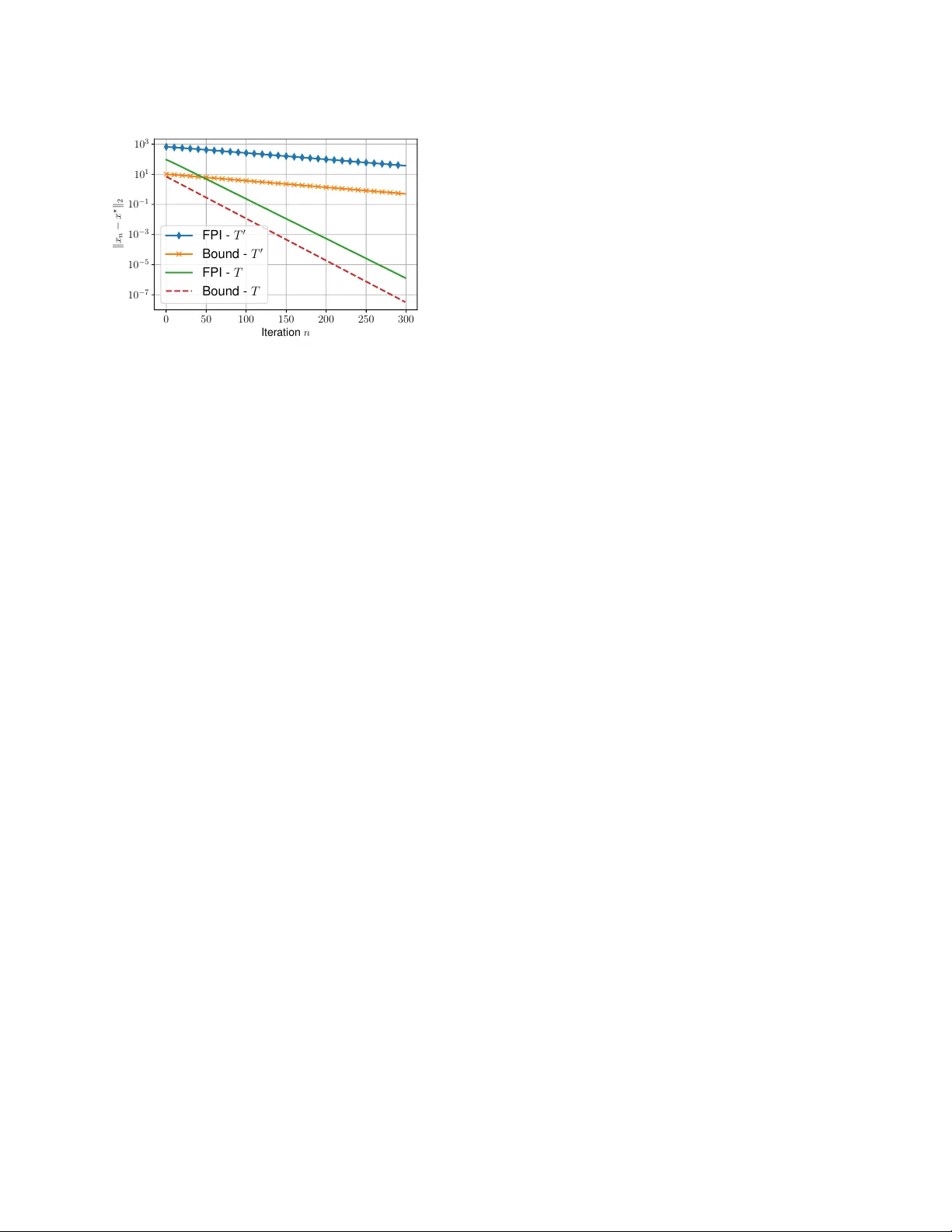
SPECTRAL RADII OF ASYMPTO TIC MAPPINGS AND THE CONVERGENCE SPEED OF THE ST AND ARD FIXED POINT ALGORITHM R. L. G. Cavalcante and S. Sta ´ nczak Fraunhofer Heinrich Hertz Institute and T echnical University of Berlin ABSTRA CT Important problems in wireless networks can often be solv ed by computing fix ed points of standard or contractiv e interfer- ence mappings, and the con ventional fixed point algorithm is widely used for this purpose. Knowing that the mapping used in the algorithm is not only standard but also contractiv e (or only contractive) is valuable information because we obtain a guarantee of geometric con vergence rate, and the rate is re- lated to a property of the mapping called modulus of contrac- tion. T o date, contractiv e mappings and their moduli of con- traction have been identified with case-by-case approaches that can be difficult to generalize. T o address this limitation of existing approaches, we show in this study that the spec- tral radii of asymptotic mappings can be used to identify an important subclass of contracti ve mappings and also to es- timate their moduli of contraction. In addition, if the fixed point algorithm is applied to compute fix ed points of positi ve concav e mappings, we show that the spectral radii of asymp- totic mappings provide us with simple lower bounds for the estimation error of the iterates. An immediate application of this result prov es that a kno wn algorithm for load estimation in wireless networks becomes slo wer with increasing traffic. Index T erms — Contractiv e interference mappings, stan- dard interference mappings, con vergence rate 1. INTRODUCTION The objecti ve of this study is to in vestigate conv ergence prop- erties of the sequence ( x n ) n ∈ N generated by the follo wing instance of the standar d fixed point algorithm : x n +1 = T ( x n ) , (1) where x 1 ∈ R N + is an arbitrary initial point; R N + denotes the set of nonnegati ve vectors of dimension N ; and T : R N + → R N + is a standard interference mapping as defined in [ 1 ] or a ( c -)contractiv e mapping as defined in [ 2 ], or both. Previous studies [ 1 , 2 ] hav e sho wn that, if T is a standard interference mapping with Fix( T ) := { x ∈ R N + | x = T ( x ) } 6 = ∅ or a contractiv e mapping, then Fix( T ) is a singleton, and the sequence generated by ( 1 ) conver ges to the fix ed point x ? ∈ Fix( T ) . The algorithm in ( 1 ) plays a piv otal role in man y power and resource allocation mechanisms in wire- less netw orks [ 1 – 14 ], so establishing its con vergence rate is a problem of significant practical importance [ 2 , 5 , 6 , 8 ]. If the mapping T in ( 1 ) is only a standard interference mapping, then the fixed point algorithm can be particularly This research was supported by Grant ST A 864/9-1 from the German Re- search Foundation (DFG). This work has also been performed in the framework of the Horizon 2020 project ONE5G (ICT - 760809) receiving funds from the European Union. The authors would like to acknowledge the contributions of their colleagues in the project, although the vie ws expressed in this contrib ution are those of the authors and do not necessarily represent the project. slow because we can hav e sublinear conv ergence rate [ 2 , Ex- ample 1]. This fact has motiv ated the authors of [ 2 ] to in- troduce the abo ve-mentioned c -contracti ve interference map- pings, where c ∈ [0 , 1[ is an intrinsic property of the map- ping called modulus of contr action (see Definition 1 in Sect. 2 for details). In particular , by knowing that the mapping T in ( 1 ) is contractiv e, we rule out the possibility of sublin- ear con vergence rate. More precisely , by using ( 1 ) with a c -contractiv e mapping T to estimate x ? ∈ Fix( T ) , the error k x n − x ? k of the estimate x n at iteration n ∈ N is upper bounded by [ 2 ] k x n − x ? k ≤ c n − 1 B k x 1 − x ? k , (2) where B ∈ R + is a parameter that depends on the choice of the norm k · k . Therefore, with knowledge of the small- est modulus of contraction c , we can ev aluate whether the recursion in ( 1 ) can obtain a good estimate of x ? ∈ Fix( T ) with fe w iterations. Howe ver , simple and general approaches to v erify whether a mapping is contractiv e ha ve not been pro- posed in [ 2 ]. Furthermore, that study has not considered com- putationally ef ficient methods to obtain the smallest modulus of contraction. Against this background, in this study we show that infor- mation about the smallest modulus of contraction of a con vex contractiv e interference mapping can be obtained from the spectral radius of its associated asymptotic mapping, a con- cept recently introduced in [ 15 , 16 ]. W e further show easily verifiable suf ficient conditions to determine whether a giv en mapping is contractiv e. In addition, we giv e lo wer bounds for the estimation error of the iterates in ( 1 ) with positive con- cav e mappings that are not necessarily contracti ve. Unlike the bounds in previous studies [ 5 , Ch. 5] [ 2 , 6 ], those deri ved here only depend on parameters that are easy to compute in practice, and we do not assume that the mappings used in ( 1 ) are constructed by combining a finite number of affine map- pings. As an application of the results in this study , we show bounds for the estimation error of the iterates generated by ( 1 ) with a nonlinear mapping widely used to estimate the load of base stations in wireless netw orks [ 3 , 8 , 17 – 20 ]. In this appli- cation, our bounds give a formal proof that the algorithm for load estimation becomes slower with increasing traf fic. 2. PRELIMINARIES In this section we establish notation and revie w the main mathematical concepts used in this study . In more detail, the sets of nonnegati ve and positi ve reals are denoted by , respec- tiv ely , R + and R ++ . Inequalities in volving vectors should be understood coordinate-wise. A norm k · k in R N is mono- tone if ( ∀ x ∈ R N + )( ∀ y ∈ R N + ) x ≤ y ⇒ k x k ≤ k y k . W e say that a sequence ( x n ) n ∈ N ⊂ R N + con verges to x ? if lim n →∞ k x n − x ? k = 0 for some (and hence for ev- ery) norm k · k in R N , and in this case we also write x n → x ? . Giv en a norm k · k and a sequence ( x n ) n ∈ N ⊂ R N + , if ( ∃ c ∈ [0 , 1[)( ∃ B ∈ R + )( ∀ n ∈ N ) k x n +1 − x ? k ≤ c n B k x 1 − x ? k , then we say that ( x n ) n ∈ N (or the algorithm generating the sequence) con verges geometrically fast . The (effective) domain of a function f : R N → R ∪ {−∞ , ∞} is the set given by dom f := { x ∈ R N | f ( x ) < ∞} , and f is pr oper if dom f 6 = ∅ and ( ∀ x ∈ R N ) f ( x ) > −∞ . Definition 1. (Standard and c -contractiv e interference map- pings:) Consider the following statements for a continuous mapping T : R N + → R N ++ : (i) [monotonicity] ( ∀ x ∈ R N + )( ∀ y ∈ R N + ) x ≥ y ⇒ T ( x ) ≥ T ( y ) (ii) [scalability] ( ∀ x ∈ R N + ) ( ∀ α > 1) αT ( x ) > T ( α x ) . (iii) [contractivity] ( ∃ ( v , c ) ∈ R N ++ × [0 , 1[)( ∀ x ∈ R N + )( ∀  > 0) T ( x +  v ) ≤ T ( x ) + c v If (i) and (ii) are satisfied, then T is said to be a standar d interfer ence mapping [ 1 ]. If T satisfies (i) and (iii), then T is called a contractive interference mapping . In this case, if a scalar c with the property in (iii) is kno wn, then c is called a modulus of contr action for T , and we also say that T is c - contractive to emphasize this kno wledge [ 2 ]. A mapping T : R N + → R N + is said to be concave (re- spectiv ely con vex ) if each coordinate function is concav e (re- spectiv ely con ve x). Recall from the Introduction that the set of fixed points of a mapping T : R N + → R N + is denoted by Fix( T ) := { x ∈ R N + | T ( x ) = x } . If T is contractive, then Fix( T ) is a singleton [ 2 ]. If T is a standard interfer- ence mapping, then Fix( T ) is either a singleton or the empty set [ 1 ]. Giv en a proper function f : R N → R ∪ {∞} , we say that f ∞ : R N → R ∪ {−∞} ∪ {∞} : x 7→ lim inf t →∞ , y → x f ( t y ) /t is the asymptotic function asso- ciated with f [ 21 , Ch. 2.5], and note that f ∞ is positi vely homogeneous [i.e., ( ∀ x ∈ R N )( ∀ α > 0) f ( α x ) = α f ( x ) ] and lower semicontinuous [ 21 , Proposition 2.5.1]. Asymp- totic functions associated with conv ex functions have the following useful property: Fact 1. [ 21 , Proposition 2.5.2] Let f : R N → R ∪ {∞} be proper , lower semicontinuous, and con vex. Then ( ∀ d ∈ R N ) f ∞ ( d ) = sup { f ( x + d ) − f ( x ) | x ∈ dom f } . In the next Lemma, we sho w a result related to Fact 1 for nonnegati ve concave functions. W e omit the proof because of the space limitation. Lemma 1. Let f : R N → R + ∪ {∞} be a function such that dom f = R N + . Assume that f is continuous and concave if r estricted to its domain. Then ( ∀ d ∈ dom f ) f ∞ ( d ) = inf { f ( x + d ) − f ( x ) | x ∈ dom f } . W e now introduce a slight generalization of the concept of asymptotic mappings giv en in [ 15 , 16 ]. Definition 2. (Asymptotic mappings:) Let T : R N + → R N + : x 7→ [ T (1) ( x ) , · · · , T ( N ) ( x )] be a mapping such that, for each i ∈ { 1 , . . . , N } , the function T ( i ) : R N → R + ∪ {∞} is proper and dom T ( i ) = dom T ( i ) ∞ = R N + . For these mappings, we say that T ∞ : R N + → R N + : x 7→ [ T (1) ∞ ( x ) , · · · , T ( N ) ∞ ( x )] is the asymptotic mapping associ- ated with T . If T : R N + → R N + is a continuous concave mapping, a standard interference mapping, or a conv ex mapping ha v- ing an asymptotic mapping, then we can use the follow- ing analytical simplification to obtain the asymptotic map- ping [ 15 , 16 ] [ 21 , Corollary 2.5.3]: ( ∀ x ∈ R N + ) T ∞ ( x ) = lim t →∞ (1 /t ) T ( t x ) . The spectral radius ρ ( T ∞ ) of a con- tinuous and monotonic (see Definition 1 (i)) asymptotic mapping T ∞ is the value giv en by ρ ( T ∞ ) := sup { λ ∈ R + | ( ∃ x ∈ R N + \{ 0 } ) T ∞ ( x ) = λ x } ∈ R + , and we recall that there always e xists an eigen vector x ∈ R N + satisfying ρ ( T ∞ ) x = T ∞ ( x ) [ 22 ]. The next fact is crucial to pro ve our main contributions. Fact 2. [ 15 ] Let T : R N + → R N ++ be a standard interference mapping. Then Fix( T ) 6 = ∅ if and only if ρ ( T ∞ ) < 1 . 3. CONVERGENCE PROPER TIES OF THE ST AND ARD FIXED POINT ALGORITHM By ( 2 ), the sequence generated by ( 1 ) with a c -contracti ve mapping T has the desirable property of conv erging geomet- rically fast, and the con vergence speed is directly related to the modulus of contraction c . Therefore, identifying contrac- tiv e mappings and estimating their moduli of contraction are important tasks. In Sect. 3.2 , we prov e that the spectral radii of asymptotic mappings can be used for these tasks if T is con vex. Then, in Sect. 3.3 we show that, if the fix ed point al- gorithm in ( 1 ) is used with an arbitrary (continuous) positive concav e mapping T , then the spectral radius of T ∞ provides us with information about the fastest conv ergence speed we can expect from the algorithm. All these results are especially useful if we can easily ev aluate the spectral radii of arbitrary asymptotic mappings, so we start by showing in Sect. 3.1 simple algorithms for this purpose. These algorithms also en- able us to obtain information about an eigen vector associated with the spectral radius. 3.1. Spectral radius of asymptotic mappings Let T ∞ : R N + → R N + be a continuous asymptotic mapping associated with a continuous mapping T : R N + → R N + sat- isfying property (i) in Definition 1 . It can be verified that T ∞ also satisfies property (i). If T ∞ is in addition concave and primitiv e, in the sense that 1 ( ∀ x ∈ R N + \{ 0 } )( ∃ p ∈ N )( ∀ m ≥ p ) T m ∞ ( x ) > 0 , then the sequence ( x n ) n ∈ N gen- erated by x n +1 = 1 k T ∞ ( x n ) k T ∞ ( x n ) , x 1 ∈ R N + \{ 0 } (3) with an arbitrary monotone norm k · k conv erges to a point x ? ∈ R N ++ such that T ∞ ( x ? ) = k T ∞ ( x ? ) k x ? and k x ? k = 1 [ 23 , 24 ]. Therefore, by [ 22 , Lemma 3.3], we conclude that ρ ( T ∞ ) = k T ∞ ( x ? ) k . In practical terms, the iteration in ( 3 ) is a simple algorithm to compute the spectral radius and a corresponding eigenv ector of an asymptotic mapping, pro- vided that the assumptions mentioned above are valid. In more challenging cases in which existing results such as those in [ 23 , 24 ] does not necessarily guarantee conv ergence of ( 3 ) to a point x ? satisfying ρ ( T ∞ ) = k T ∞ ( x ? ) k , we propose an approach based on the following result (the proof is omitted because of the space limitation): 1 T m ∞ denotes the m -fold composition of T ∞ with itself. Proposition 1. Let T ∞ : R N + → R N + be a continuous asymp- totic mapping satisfying the monotonicity property in Defini- tion 1 , and consider the mapping T  : R N + → R N + : x 7→ T ∞ ( x ) +  1 , where 1 ∈ R N denotes the vector of ones and  > 0 is arbitr ary . F or a given parameter p > 0 , let the sequence ( x p,n ) n ∈ N be generated by x p,n := p k T  ( x p,n ) k T  ( x p,n ) , (4) wher e x p, 1 ∈ R N + is arbitrary , and k · k is a monotone norm. Then we have the following: (i) T  is a standar d interference mapping . (ii) F or every p > 0 , the sequence ( x p,n ) n ∈ N con- ver ges to a point x ? p ∈ R N ++ satisfying T  ( x ? p ) = ( k T  ( x ? p ) k /p ) x ? p and k x ? p k = p . (iii) ( ∀ p > 0) ρ ( T ∞ ) ≤ k T  ( x ? p ) k /p (iv) lim p →∞ k T  ( x ? p ) k /p = ρ ( T ∞ ) (v) If ( p n ) ⊂ R ++ is a sequence satisfying lim n →∞ p n = ∞ , then any accumulation point of ( x ? p n ) n ∈ N is an eigen vector of T ∞ associated with the eigen value ρ ( T ∞ ) . In simple terms, Proposition 1 (iii)-(iv) shows that the spectral radius ρ ( T ∞ ) of any asymptotic mapping T ∞ that is monotonic and continuous can be estimated with an y ar - bitrary precision by using ( 4 ). Informally , giv en an arbitrary scalar  > 0 , if n ∈ N and p ∈ R ++ are sufficiently large, then ρ ( T ∞ ) ≈ k T  ( x p,n ) k /p , where ( x p,n ) n ∈ N is the se- quence generated by ( 4 ). Furthermore, by assuming that ( x ? p n ) n ∈ N in Proposition 1 (v) con ver ges, then x p,n with the abov e parameters is an approximation of an eigenv ector of T ∞ associated with the spectral radius ρ ( T ∞ ) . 3.2. Conv ex mappings Checking whether a continuous and monotonic mapping T : R N + → R N ++ is c -contractiv e may be challenging because proving the existence of a tuple ( v , c ) ∈ R N ++ × [0 , 1[ with the property in Definition 1 (iii) may be dif ficult. Howe ver , as we show in the next proposition, if T is conv ex (as common in many robust wireless resource allocation problems [ 13 , 14 ]), then knowledge of the spectral radius of T ∞ , assuming that T ∞ exists, can be used to determine whether T is contractive. Proposition 2. Let T : R N + → R N ++ be a continuous conve x mapping that has an associated continuous asymptotic map- ping T ∞ : R N + → R N + . Further assume the following: (i) ther e e xists a (strictly) positive vector v ∈ R N ++ such that T ∞ ( v ) = ρ ( T ∞ ) v , (ii) T satisfies the monotonicity pr operty in Definition 1 , and (iii) ρ ( T ∞ ) < 1 . Then T is c -contractive for any c ∈ [ ρ ( T ∞ ) , 1[ ⊂ [0 , 1[ . Pr oof. W e only hav e to sho w that the property in Defini- tion 1 (iii) can be satisfied with c = ρ ( T ∞ ) ≥ 0 . T o this end, let v ∈ R N ++ be a v ector with the property in assumption (i). Now , by Fact 1 and positiv e homogeneity of asymptotic mappings, we deduce ( ∀  > 0)( ∀ x ∈ R N + ) T ( x +  v ) ≤ T ( x ) + T ∞ (  v ) = T ( x ) + ρ ( T ∞ )  v , and the claim fol- lows. W e note that there are many simple results to verify as- sumption (i) in Proposition 2 without explicitly computing a so-called (nonlinear) eigen vector v ∈ R ++ [ 25 ]. In addition, neither assumption (ii) nor assumption (iii) can be dropped. The former is required because of the definition of contractive mappings, and the latter is also necessary because, as shown below , the spectral radius of the asymptotic mapping T ∞ as- sociated with a c -contractiv e mapping T is a lower bound for the modulus of contraction c ∈ [0 , 1[ . Proposition 3. Let T : R N + → R N ++ be c -contractive and con vex. Then T has a continuous asymptotic mapping T ∞ : R N + → R N + satisfying ρ ( T ∞ ) ≤ c ∈ [0 , 1[ . Pr oof. By definition, if T is c -contractive, there exists ( v , c ) ∈ R N ++ × [0 , 1[ such that ( ∀  > 0)( ∀ x ∈ R N + ) T ( x +  v ) − T ( x ) ≤ c v . (5) Denote by T ( i ) : R N + → R N ++ the i th coordinate function of the mapping T ; i.e., ( ∀ x ∈ R N + )[ T (1) ( x ) , · · · , T ( N ) ( x )] := T ( x ) . Since T is continuous and con vex, by F act 1 we have ( ∀ d ∈ R N + )( ∀ i ∈ { 1 , · · · , N } ) T ( i ) ∞ ( d ) := sup { T ( i ) ( x + d ) − T ( i ) ( x ) | x ∈ R N + } . (6) T o prove that T ∞ ( x ) := [ T (1) ∞ ( x ) , · · · , T ( N ) ∞ ( x )] ≥ 0 for x ∈ R N + is the asymptotic mapping associated with T (in the sense of Definition 2 ), we need to sho w that dom T ( i ) ∞ = R N + for each i ∈ { 1 , . . . , N } . T o this end, take the coordi- natewise supremum in ( 5 ) over x ∈ R N + and apply ( 6 ) with d =  v and an arbitrary  > 0 to obtain [ T (1) ∞ (  v ) , · · · , T ( N ) ∞ (  v )] =: T ∞ (  v ) ≤ c v . (7) By positivity of v , for an arbitrary x ∈ R N + , there exists η > 0 such that x ≤ η v . Since  > 0 in ( 7 ) can be chosen arbitrarily , we can use η =  and monotonicity of T to deduce T ∞ ( x ) ≤ T ∞ ( η v ) ≤ cη v ∈ R N + . As a result, we hav e T ( i ) ∞ ( x ) < ∞ for all x ∈ R N + and all i ∈ { 1 , . . . , N } as claimed. (W e can also sho w that T ∞ is continuous in R N + , but we omit the proof because of the space limitation.) With the inequality in ( 7 ) and continuity of T ∞ , we also obtain ρ ( T ∞ ) ≤ c by [ 22 , Lemma 3.3], and the proof is complete. W e now show a useful relation between contractive and standard interference mappings. From a practical perspec- tiv e, the ne xt result and ( 2 ) rev eal that man y existing iterativ e algorithms for power control in wireless networks conv erge geometrically fast. Furthermore, the inequality in ( 2 ), Propo- sition 2 , and Proposition 3 show that the concept of spectral radius of asymptotic mappings provides us with information about the con vergence speed of these algorithms. Proposition 4. Let T : R N + → R N ++ be a con vex standard interfer ence mapping. Then ρ ( T ∞ ) < 1 is a sufficient and necessary condition for T to be contractive. Pr oof. By F act 2 , if ρ ( T ∞ ) ≥ 1 , then Fix( T ) = ∅ , so T can- not be contracti ve because contracti ve mappings hav e a fixed point [ 2 ]. Therefore, ρ ( T ∞ ) < 1 is a necessary condition. T o prov e sufficiency , we only need to show that property (iii) in Definition 1 is satisfied if ρ ( T ∞ ) < 1 . By Fact 2 , if ρ ( T ∞ ) < 1 then there exists x ? ∈ R N ++ such that x ? = T ( x ? ) . By [ 16 , Lemma 1(ii)] and T ∞ ( x ? ) = lim t →∞ T ( t x ? ) /t [ 21 , Corol- lary 2.5.3], we hav e T ∞ ( x ? ) < T ( x ? ) = x ? . As a result, there exists c ∈ [0 , 1[ such that T ∞ ( x ? ) ≤ c x ? for all  > 0 . Therefore, by the positive homogeneity of asymp- totic functions, we have T ∞ (  x ? ) ≤ c x ? for all  > 0 . By Fact 1 , we conclude that T ( x +  x ? ) − T ( x ) ≤ T ∞ (  x ? ) ≤ c x ? for ev ery x ∈ R N + , and the desired result follows. 3.3. Concave mappings W e now proceed to study con vergence properties of the al- gorithm in ( 1 ) with (continuous) positive concave mappings, and we recall that these mappings are also standard [ 8 , Propo- sition 1]. In particular, the ne xt proposition pro ves that the spectral radii of asymptotic mappings can be used to obtain a lower bound for the estimation error of the sequence gener- ated by ( 1 ) – see the inequality in ( 8 ). Proposition 5. Assume that T : R N + → R N ++ is continuous and concave with ∅ 6 = Fix( T ) =: { x ? } , and denote by v ∈ R N + \{ 0 } any vector satisfying T ∞ ( v ) = ρ ( T ∞ ) v (a vector with this pr operty always exists [ 22 ]). T o simplify notation, define ρ := ρ ( T ∞ ) < 1 , where the inequality follows from F act 2 . Then each of the following holds: (i) ( ∀ n ∈ N )( ∀  > 0) T n ( x ? +  v ) ≥ x ? + ρ n  v (ii) ( ∀ n ∈ N )( ∀  > 0) x ? ≥  v ⇒ T n ( x ? −  v ) ≤ x ? − ρ n  v (iii) If x 1 ∈ R N + is such that x 1 ≤ x ? −  v or x 1 ≥ x ? +  v ≥ 0 for some  > 0 , then ρ n  k v k ≤ k T n ( x 1 ) − x ? k → 0 (8) for any monotone norm k · k and every n ∈ N . Pr oof. (i) W e prov e the result by induction on n . By Lemma 1 , we know that ( ∀ d ∈ R N + )( ∀ x ∈ R N + ) T ∞ ( d ) ≤ T ( x + d ) − T ( x ) . (9) In particular , for d =  v and x = x ? with  > 0 arbitrary , we have ρ v = T ∞ (  v ) ≤ T ( x ? +  v ) − x ? , which shows that the desired inequality is valid for n = 1 . Now assume that T n ( x ? +  v ) ≥ x ? + ρ n  v is valid for an arbitrary n ∈ N . As a consequence of the monotonicity of T , we ha ve T n +1 ( x ? +  v ) ≥ T ( x ? + ρ n  v ) . (10) Now substitute d = ρ n  v and x = x ? into ( 9 ) and use the positive homogeneity property of T ∞ to verify that ρ n +1  v = T ∞ ( ρ n  v ) ≤ T ( x ? + ρ n  v ) − x ? , and thus ρ n +1  v + x ? ≤ T ( x ? + ρ n  v ) . Combining this inequality with that in ( 10 ), we obtain the desired result T n +1 ( x ? +  v ) ≥ x ? + ρ n +1  v , and the proof is complete. (ii) The proof is similar to that in part (i), so it is omitted for bre vity . (iii) If x 1 ≥ x ? +  v ≥ x ? for some  > 0 , then ( ∀ n ∈ N ) T n ( x 1 ) ≥ T n ( x ? +  v ) ≥ T n ( x ? ) = x ? by monotonicity of T . Therefore, ( ∀ n ∈ N ) T n ( x 1 ) − x ? ≥ T n ( x ? +  v ) − x ? ≥ ρ n  v , where the last inequality fol- lows from part (i). Monotonicity of the norm k · k now shows that ( ∀ n ∈ N ) k T n ( x 1 ) − x ? k ≥ ρ n  k v k . In addition, posi- tiv e concave mappings are standard interference mappings [ 8 , Proposition 1], so k T n ( x 1 ) − x ? k → 0 by [ 1 , Theorem 2], and the proof for x 1 ≥ x ? +  v ≥ x ? is complete. W e skip the proof for x 1 ≤ x ? −  v ≤ x ? because it is similar . 4. NUMERICAL EXAMPLE T o illustrate the results obtained in the previous section in a concrete application, we study the con vergence speed of a well-known algorithm for load estimation in wire- less networks [ 3 , 8 , 11 , 15 , 17 – 19 ]. The algorithm is sim- ply the iteration in ( 1 ) with the concav e mapping given by T : R N + → R N ++ : x 7→ [ t 1 ( x ) , · · · , t N ( x )] , where, for all i ∈ { 1 , . . . , N } =: M and all x ∈ R N + , t i ( x ) := X j ∈N i d j K B log 2    1 + p i g i,j P k ∈M\{ i } x k p k g k,j + σ 2    , (11) M is the set of base stations, N i 6 = ∅ is the set of users con- nected to base station i , d j ∈ R ++ is the traffic (in bits/s) re- quested by the j th user , K ∈ N is number of resource blocks in the system, B ∈ R ++ is the bandwidth per resource block, p i > 0 is the transmit power per resource block of base sta- tion i , g i,j > 0 is the pathloss between base station i and user j , and σ 2 > 0 is the noise power per resource block. The i th component x ? i of the fixed point x ? ∈ Fix( T ) , if it e xists, shows the fraction of resource blocks that base station i re- quires to satisfy the traffic demand of its users. Although we cannot ha ve x ? i > 1 in real network deployments, knowledge of these values is useful to rank base stations according to the unserved traffic demand [ 18 ]. See [ 3 , 8 , 11 , 15 , 17 , 18 , 20 ] for additional details on the load estimation problem. The asymptotic mapping associated with T is gi ven by [ 15 ] T ∞ : R N + → R N + : x 7→ diag( p ) − 1 M diag ( p ) x , where diag ( p ) ∈ R N × N + is a diagonal matrix with diagonal elements obtained from the components of the power vector p := [ p 1 , . . . , p N ] , and the component [ M ] i,k of the i th row and k th column of the matrix M ∈ R N × N + is gi ven by [ M ] i,k = 0 if i = k or [ M ] i,k = P j ∈N i ln(2) d j g k,j / ( K B g i,j ) otherwise. The asymptotic mapping T ∞ is linear, so ρ ( T ∞ ) is simply the spectral radius of the matrix M . W ith the results in Proposition 5 , we can prove that the conv ergence rate of the recursion in ( 1 ) is expected to decrease with increasing traf fic. T o this end, let T 0 ( x ) = β T ( x ) for every x ∈ R N + , where β ∈ R ++ is a design pa- rameter . This new mapping T 0 can be obtained, for example, by scaling uniformly the traf fic demand of ev ery user by a factor β , and we assume that ρ ( T ∞ ) < 1 . W e can verify that ρ ( T 0 ∞ ) = β ρ ( T ∞ ) > 0 . As a result, in light of the bound in ( 8 ), by increasing β , the algorithm is expected to become increasingly slow as ρ ( T 0 ∞ ) = β ρ ( T ∞ ) < 1 approaches the value one. (The algorithm diver ges if β ρ ( T ∞ ) ≥ 1 .) Fig. 1 illustrates the above points. It shows the estimation error k x n − x ? k 2 of the fix ed point iteration (FPI) in ( 1 ) with x 1 = 0 and the bound in Proposition 5 (iii) for the mappings T and T 0 described above. The parameter β > 1 for T 0 was chosen to satisfy ρ ( T 0 ∞ ) = 0 . 99 . For the construction of T , we use a scenario similar to that in [ 8 , Sect. V -A]. Briefly , we obtained snapshots of a network with 1,500 users request- ing a traffic of 300 kbps each, and we picked one snapshot with ρ ( T ∞ ) < 0 . 99 , in which case we also have Fix( T ) 6 = ∅ as an implication of Fact 2 . Other parameters of the simula- tion were the same as those in [ 8 , T able I]. T o compute the bound in ( 8 ) for T , we set the vector v to the right eigenv ector of diag ( p ) − 1 M diag ( p ) (obtained by using ( 3 )) associated with the eigen value ρ ( T ∞ ) . In turn, the scalar  in ( 8 ) was set to the largest positi ve real such that x ? −  v ∈ R N + . The bound for T 0 was constructed in a similar way . As expected, the numerical results in Fig. 1 are consistent with the theoret- ical findings. 0 50 100 150 200 250 300 Iter ation n 10 − 7 10 − 5 10 − 3 10 − 1 10 1 10 3 k x n − x ? k 2 FPI - T 0 Bound - T 0 FPI - T Bound - T Fig. 1 : Estimation error as a function of the number of itera- tions. 5. CONCLUSIONS AND FINAL REMARKS W e have shown that knowledge of the spectral radius of asymptotic mappings is useful to relate standard and contrac- tiv e interference mappings, and with this knowledge we also obtain information about the conv ergence speed of widely used instances of the recursion in ( 1 ). One advantage of the analysis shown here o ver existing results in the literature is that we do not assume the mapping T in ( 1 ) to be constructed by combining a finite number of affine functions. Further- more, unlike previous results, in the proposed approaches the parameters used to obtain bounds for the con ver gence speed are easy to estimate. The bounds deri ved here show , for e xample, that the con verge speed of a well-known iter - ativ e algorithm for load estimation in wireless networks is expected to decrease with increasing traf fic. 6. REFERENCES [1] R. D. Y ates, “ A framework for uplink power control in cellular radio systems, ” IEEE J. Select. Ar eas Commun. , vol. 13, no. 7, pp. pp. 1341–1348, Sept. 1995. [2] Hamid Reza Feyzmahdavian, Mikael Johansson, and Themistoklis Charalambous, “Contracti ve interference functions and rates of con vergence of distributed power control laws, ” IEEE T ransactions on W ireless Commu- nications , vol. 11, no. 12, pp. 4494–4502, 2012. [3] R. L. G. Ca valcante, S. Sta ´ nczak, M. Schubert, A. Eisenbl ¨ ater , and U. T ¨ urke, “T o ward energy-ef ficient 5G wireless communication technologies, ” IEEE Sig- nal Pr ocessing Mag. , vol. 31, no. 6, pp. 24–34, Nov . 2014. [4] Chin Keong Ho, Di Y uan, Lei Lei, and Sumei Sun, “On power and load coupling in cellular networks for energy optimization, ” IEEE T rans. W ir eless Commun. , v ol. 14, no. 1, pp. 500–519, Jan. 2015. [5] Martin Schubert and Hoger Boche, Interfer ence Cal- culus - A General F ramework for Interfer ence Man- agement and Network Utility Optimization , Springer , Berlin, 2011. [6] Ching-Y ao Huang and Roy D Y ates, “Rate of con- ver gence for minimum po wer assignment algorithms in cellular radio systems, ” W ir eless Networks , vol. 4, no. 3, pp. 223–231, 1998. [7] R. L. G. Cav alcante and S. Stanczak, “Peak load min- imization in load coupled interference network, ” in IEEE International Confer ence on Acoustics, Speech and Signal Pr ocessing (ICASSP) , March 2017, pp. 3729–3733. [8] Renato L. G. Cav alcante, Y uxiang Shen, and Slawomir Sta ´ nczak, “Elementary properties of positi ve concave mappings with applications to network planning and optimization, ” IEEE T rans. Signal Processing , vol. 64, no. 7, pp. 1774–1873, April 2016. [9] R. L. .G. Cav alcante, M. Kasparick, and S. Sta ´ nczak, “Max-min utility optimization in load coupled interfer- ence networks, ” IEEE T rans. W ireless Commun. , vol. 16, no. 2, pp. 705–716, Feb . 2017. [10] S. Sta ´ nczak, M. Wiczano wski, and H. Boche, Funda- mentals of Resour ce Allocation in W ireless Networks , Foundations in Signal Processing, Communications and Networking. Springer , Berlin Heidelberg, 2nd edition, 2009. [11] Albrecht Fehske, Henrik Klessig, Jens V oigt, and Ger- hard Fettweis, “Concurrent load-a ware adjustment of user association and antenna tilts in self-organizing ra- dio networks, ” IEEE T rans. V eh. T echnol. , , no. 5, June 2013. [12] Carl J Nuzman, “Contraction approach to power control, with non-monotonic applications, ” in IEEE GLOBECOM 2007-IEEE Global T elecommunications Confer ence . IEEE, 2007, pp. 5283–5287. [13] Holger Boche and Martin Schubert, “Concav e and con- ve x interference functions – general characterizations and applications, ” IEEE T ransactions on Signal Pr o- cessing , vol. 56, no. 10, pp. 4951–4965, 2008. [14] Martin Schubert and Holger Boche, “Robust resource allocation, ” in Information Theory W orkshop, 2006. ITW’06 Chengdu. IEEE . IEEE, 2006, pp. 556–560. [15] R. L. G. Cavalcante and S. Sta ´ nczak, “The role of asymptotic functions in network optimization and fea- sibility studies, ” in IEEE Global Conference on Signal and Information Pr ocessing (GlobalSIP) , Nov . 2017, to appear . [16] R. L. G. Cavalcante and S Sta ´ nczak, “Performance lim- its of solutions to netw ork utility maximization prob- lems, ” , 2017. [17] K. Majewski and M. Koonert, “Conservati ve cell load approximation for radio networks with Shannon chan- nels and its application to L TE network planning, ” in T elecommunications (AICT), 2010 Sixth Advanced In- ternational Confer ence on , May 2010, pp. 219 –225. [18] Ioana Siomina and Di Y uan, “ Analysis of cell load coupling for L TE network planning and optimization, ” IEEE T rans. W ir eless Commun. , vol. 11, no. 6, pp. 2287–2297, June 2012. [19] Iana Siomina and Di Y uan, “On optimal load setting of load-coupled cells in heterogeneous L TE networks, ” in Communications (ICC), 2014 IEEE International Con- fer ence on . IEEE, 2014, pp. 1254–1259. [20] C Ho, Di Y uan, and Sumei Sun, “Data offloading in load coupled networks: A utility maximization frame- work, ” IEEE T rans. W ireless Commun. , vol. 13, no. 4, pp. 1921–1931, April 2014. [21] A. Auslender and M. T eboulle, Asymptotic Cones and Functions in Optimization and V ariational Inequalities , Springer , New Y ork, 2003. [22] Roger D Nussbaum, “Conv exity and log con ve xity for the spectral radius, ” Linear Algebr a and its Applica- tions , vol. 73, pp. 59–122, 1986. [23] Ulrich Krause, “Perron’ s stability theorem for non- linear mappings, ” Journal of Mathematical Economics , vol. 15, no. 3, pp. 275–282, 1986. [24] Ulrich Krause, “Concave Perron–Frobenius theory and applications, ” Nonlinear Analysis: Theory , Methods & Applications , vol. 47, no. 3, pp. 1457–1466, 2001. [25] St ´ ephane Gaubert and Jeremy Gunawardena, “The Perron-Frobenius theorem for homogeneous, monotone functions, ” T ransactions of the American Mathematical Society , vol. 356, no. 12, pp. 4931–4950, 2004.