Estimating uncertainty of earthquake rupture using Bayesian neural network
Bayesian neural networks (BNN) are the probabilistic model that combines the strengths of both neural network (NN) and stochastic processes. As a result, BNN can combat overfitting and perform well in applications where data is limited. Earthquake ru…
Authors: Sabber Ahamed, Md Mesbah Uddin
E S T I M A T I N G U N C E RT A I N T Y O F E A RT H Q UA K E R U P T U R E U S I N G B A Y E S I A N N E U R A L N E T W O R K A P R E P R I N T Sabber Ahamed 1 , Md Mesbah Uddin 2 1 sabbers@gmail.com , 2 Mesbahuddin1991@gmail.com April 13, 2023 A B S T R AC T W e introduce a ne w and practical artificial intelligence called a shallo w explainable Bayesian neural network, specifically designed to tackle the challenges of limited data and high computational costs in earthquake rupture studies. Earthquake researchers often face the issue of insufficient data, which makes it dif ficult to determine the actual reasons behind an earthquake rupture. Furthermore, relying on trial-and-error simulations can be computationally expensi ve. W e used 2,000 2D earthquake rupture simulations to train and test our model. Each simulation took about two hours on eight processors and had v arying stress conditions and friction parameters. The BNN outperformed a standard neural network by 2.34 % . Upon analyzing the BNN’ s learned parameters, we found that normal stresses play a crucial role in determining rupture propagation and are the most uncertain factor , followed by the dynamic friction coef ficient. Rupture propagation has more uncertainty than rupture arrest. Shear stress has a moderate impact, while geometric features like fault width and height are the least significant and uncertain factors. Our approach demonstrates the potential of the explainable Bayesian neural network in addressing the limited data and computational cost issues in earthquake rupture studies. K eywords Earthquake · Bayesian Neural network · Rupture simulation · V ariational inference 1 Introduction Hazards due to earthquakes are a threat to economic losses and human life w orldwide. A large earthquake produces high-intensity ground motion that causes damage to structures like b uildings, bridges, and dams and takes many li ves. Seismic hazard analysis (SHA) is the process used to estimate the risk associated with these damages. SHA requires A P R E P R I N T - A P R I L 1 3 , 2 0 2 3 historical earthquake information and detailed geological data. Unfortunately , there is a lack of a detailed surf ace and subsurface geologic information. Consequently , this leads to uncertainty in hazard estimation. Numerical or physical models can be used to generate synthetic data that supplement existing data. Numerical models based studies such as dynamic earthquake rupture simulations need initial parameters about the fault and the surrounding region. Such parameters can include the stress-state, frictional, and material properties of the fault. Ho wever , the initial information is also not well constrained and not always a vailable [ Duan and Oglesby , 2006 , Pe yrat et al. , 2001 , Ripperger et al. , 2008 , Kame et al. , 2003 ]. Since earthquake rupture is a highly nonlinear process, determining the right initial parameter combinations is essential for the right simulation. Different initial conditions may lead to different results; therefore, we may not capture the real scenario of an actual earthquake rupture. The parameter combinations are often determined by making simplifying assumptions or taking a trial and error approach, which is computationally expensi ve [ Douilly et al. , 2015 , Ripper ger et al. , 2008 , Peyrat et al. , 2001 ]. Therefore, high computational costs limit the applicability of simulations to integrate with seismic hazard analysis. In recent years, machine learning (ML) approaches hav e been successfully used to solve man y geophysical problems that hav e limited data and in volve computational e xpense. For e xample, Ahamed and Daub [ 2019 ] de veloped a neural network and random forest algorithms to predict if an earthquake can break through a fault with geometric heterogeneity . The authors used 1600 simulated rupture data points for dev eloping a neural network and random forest models. They were able to extract dif ferent patterns of the parameters that were responsible for earthquak e rupture. The authors find that the models can predict rupture status within a fraction of a second. A verage run time for a single simulation takes about two hours of wall-clock time on eight processors. Machine learning approaches are also used in seismic e vent detection [ Rouet-Leduc et al. , 2017 ], earthquake detec- tion [ Perol et al. , 2018 ], identifying faults from unprocessed raw seismic data [ Last et al. , 2016 ] and to predict broadband earthquake ground motions from 3D ph ysics-based numerical simulations [ P aolucci et al. , 2018 ]. All the examples show the potential of ML to solv e many unsolv ed earthquake problems. The performance of a machine learning model usually depends on the quality and the quantity of data. Bad quality or insufficient data may increase the uncertainty associated with each prediction [ Hoeting et al. , 1999 , Blei et al. , 2017 , Gal et al. , 2017 ]. Prediction uncertainty estimation is vital in many applications: diseases detection [ Leibig et al. , 2017 , Liu et al. , 2018 , Nair et al. , 2019 ], autonomous vehicle dri ving [ Kendall et al. , 2015 , McAllister et al. , 2017 , Burton et al. , 2017 ], and estimating risk [ Hoeting et al. , 1999 , T ong and K oller , 2001 , Uusitalo , 2007 ]. Therefore, calculating uncertainty is as crucial as improving model accuracy . All of the ML-based earthquak e studies mentioned above av oid prediction uncertainty estimation. T o overcome the problem of insuf ficient data of earthquake rupture, we extend the work of Ahamed and Daub [ 2019 ] using the Bayesian neural network. Unlike regular neural networks, BNN works better with a small amount of data and also provides prediction uncertainty . In this paper , we describe a workflow of (1) de veloping a BNN, (2) estimating prediction uncertainty , and (3) finding parameter combinations responsible for rupture. Identifying the source of 2 A P R E P R I N T - A P R I L 1 3 , 2 0 2 3 uncertainty is vital to understanding the physics of earthquake rupture and estimating seismic risk. W e also describe a technique that combines BNN and permutation importance to find the source of uncertainty . 2 Rupture simulations and data pr ocessing Nucleation Starts here Distance along strike (km) Distance across fault (km) 0 8 16 24 32 1.0 0.5 0.0 -0.5 -1.0 Shear Stress Slip τ s = µ s σ n τ d = µ d σ n d c = Critical slip distance x-axis y-axis (a) Rupture domain (b) Slip weakening law Fault barrier Figure 1: (a) A zoomed view of the two-dimensional fault geometry . The domain is 32 km long along the strike of the fault and 24 kilometers wide across the fault. The rupture starts to nucleate 10 km to the left of the barrier and propagates from the hypocenter tow ards the barrier, (b) Linear slip-weakening friction la w for an earthquak e fault. The fault begins to slip when the shear stress reaches or exceeds the peak strength of τ s . τ s decreases linearly with slip to a constant dynamic friction τ d ov er critical slip distance ( d c ). The shear strength is linearly proportional to the normal stress σ n , and the friction coefficient v aries with slip between µ s and µ d . In this work, we used 200 simulated earthquak e ruptures that were created by Ahamed and Daub [ 2019 ]. The simulations are a two-dimensional rupture, illustrated in figure. 1 . The domain is 32 km long and 24 km wide. Figure 1 a shows the zoomed view of the original domain for better visualization of the f ault barrier . An open-source C++ and python based library fdfault [ Daub , 2017 ] was used to generate the ruptures. The library is a finite dif ference code for numerical simulation of elastodynamic fracture and friction problems. The code solves the elastodynamic wa ve equation coupled to a friction la w describing the failure process. In each simulation, fault slip is calculated based on the initial stress conditions, the elastodynamic wa ve equations, and the frictional failure on that fault. The fault has a Gaussian geometric heterogeneity at the center . Rupture is nucleated 10 km to the left of the barrier and propagates to wards the barrier . The linear slip-weakening law determines the strength of the fault (figure. 1 b). The fault starts to break when the shear stress ( τ ) exceeds the peak strength τ s = µ s σ n , where µ s and σ n are the static friction coef ficient and normal stress, respectiv ely . Over a critical slip distance d c , the friction coefficient reduces linearly to constant dynamic friction µ d . In each simulation, eight parameters were v aried: x and y components of normal stress (sxx and syy), shear stress (sxy), dynamic friction coefficient, friction drop ( µ s − µ d ), critical slip distance ( d c ), and width and height of the fault. we used 1600 simulations to train the BNN. The remaining 400 were used to test the final model performance. The training dataset has an imbalance class proportion of rupture arrest (65 % ) and rupture propagation (35 % ). T o avoid 3 A P R E P R I N T - A P R I L 1 3 , 2 0 2 3 a bias to ward rupture arrest, we upsampled the rupture propagation examples. Before training, all the data were normalized by subtracting the mean and dividing by the standard de viation. 3 Neural network Neural networks (NN) are computing systems inspired by ho w neurons are connected in the brain [ Rosenblatt , 1958 ]. Sev eral nodes are interconnected and organized in layers in a neural network. Each node is also known as a neuron. A layer can be connected to an arbitrary number of hidden layers of arbitrary size. Howe ver , increasing the number of hidden layers not always im prove the performance b ut may force the model to generalize well on the training data but unseen (test) data, which is also known as o verfitting [ Hinton et al. , 2012 , La wrence and Giles , 2000 , Lawrence et al. , 1997 ]. As a result, selecting the number of layers and nodes in each layer is one of the challenges of using neural networks in practice. 4 Bayesian Neural network y i x i Input w 0 ij ~ N(µ, σ ) w 1 ij ~ N(µ, σ ) Figure 2: The schematic diagram shows the architecture of the Bayesian neural network used in this work. The network has one input layer with eight parameters, one hidden layer with twelve nodes, and an output layer with a single node. W eights between input and hidden layers are defined by w 0 ij , which are normally distributed. i, j are the node input and hidden layer node index. Similarly , w 1 j k is the normal distribution of weights between the hidden and the output layer . µ and σ are the mean and standard deviation. At the output node, the network produces a distribution of prediction scores between 0 and 1. In a traditional neural network, weights are assigned as a single value or point estimate. In a BNN, weights are considered as a probability distribution. These probability distributions are used to estimate the uncertainty in weights 4 A P R E P R I N T - A P R I L 1 3 , 2 0 2 3 and predictions. Figure 2 sho ws a schematic diagram of a BNN where weights are normally distributed. The final learned network weights (posterior of the weights) are calculated using Bayes theorem as: P ( W | X ) = P ( X | W ) P ( W ) P ( X ) (1) Where X is the data, P ( X | W ) is the lik elihood of observing X , given weights ( W ). P ( W ) is the prior belief of the weights, and the denominator P ( X ) is the probability of data which is also kno wn as evidence. The equation requires integrating o ver all possible v alues of the weights as: P ( X ) = Z P ( X | W ) P ( W ) dW . (2) Integrating o ver the indefinite weights in e vidence makes it hard to find a closed-form analytical solution. As a result, simulation or numerical based alternative approaches such as Monte Carlo Marko v chain (MCMC) and v ariational inference(VI) are considered. MCMC sampling is an inference method in modern Bayesian statistics, perhaps widely studied and applied in many situations. Howe ver , the technique is slow for large datasets and complex models. V ariational inference (VI), on the other hand, is faster than MCMC. It has been applied to solv e many large-scale computationally expensi ve neuroscience and computer vision problems [ Blei et al. , 2017 ]. In VI, a new distribution Q ( W | θ ) is considered that approximates the true posterior P ( W | X ) . Q ( W | θ ) is parameterized by θ o ver W and VI finds the right set of θ that minimizes the di vergence of tw o distributions through optimization: Q ∗ ( W ) = argmin θ KL [ Q ( W | θ ) || P ( W | X )] (3) In equation- 3 , KL or Kullback–Leibler di vergence is a non-symmetric and information theoretic measure of similarity (relativ e entropy) between true and approximated distributions [ Kullback , 1997 ]. The KL-di vergence between Q ( W | θ ) and P ( W | X ) is defined as: KL [ Q ( W | θ ) || P ( W | X )] = Z Q ( W | θ ) log Q ( W | θ ) P ( W | X ) dW (4) Replacing P ( W | X ) using equation- 1 we get: 5 A P R E P R I N T - A P R I L 1 3 , 2 0 2 3 KL [ Q ( W | θ ) || P ( W | X )] = Z Q ( W | θ ) log Q ( W | θ ) P ( X ) P ( X | W ) P ( W ) dW (5) = Z Q ( W | θ ) [log Q ( W | θ ) P ( X ) − log P ( X | W ) P ( W )] dW (6) = Z Q ( W | θ ) log Q ( W | θ ) P ( W ) dW + Z Q ( W | θ ) log P ( X ) dW − Z Q ( W | θ ) log P ( X | W ) dW (7) T aking the expectation with respect to Q ( W | θ ) , we get: KL [ Q ( W | θ ) || P ( W | X )] = E log Q ( W | θ ) P ( W ) + log P ( X ) − E [log P ( X | W )] (8) The above equation sho ws the dependency of log P ( X ) that makes it difficult to compute. An alternati ve objecti ve function is therefore, deriv ed by adding log P ( X ) with negati ve KL di vergence. log P ( X ) is a constant with respect to Q ( W | θ ) . The ne w function is called as the evidence of lo wer bound (ELBO) and expressed as: E LB O ( Q ) = E [log P ( X | W )] − E log Q ( W | θ ) P ( W ) (9) = E [log P ( X | W )] − K L [ Q ( W | θ ) || P ( W | X )] (10) The first term is called likelihood, and the second term is the ne gativ e KL div ergence between a variational distrib ution and prior weight distrib ution. Therefore, ELBO balances between the likelihood and the prior . The ELBO objecti ve function can be optimized to minimize the KL div ergence using dif ferent optimizing algorithms like gradient descent. 5 T rain the BNN The BNN has the same NN architecture used in Ahamed and Daub [ 2019 ] to compare the performance between them. Whether the BNN performs better or similarly to NN, BNN provides an additional adv antage of prediction uncertainty . Like NN, BNN has one input layer with eight parameters, one hidden layer with twelve nodes and one output layer (Figure 2 ). A nonlinear activ ation function ReLu [ Hahnloser et al. , 2000 ] was used at the hidden layer . ReLu passes all the v alues greater than zero and sets the neg ative output to zero. The output layer uses sigmoid activ ation function, which con verts the outputs between zero and one. Prior weights and biases are normally distrib uted with zero mean and one standard deviation. Figure 3 sho ws the log density of prior and posterior weights ( w k ij ) and biases ( b k j ). i and j are the index of the input and hidden layer nodes. i ranges from 0 to 7, and j ranges from 0 to 11. k is the index that maps two layers. As an example, w 0 15 is the weight 6 A P R E P R I N T - A P R I L 1 3 , 2 0 2 3 between the first input node and the fifth hidden node. The output node of the last layer produces a distrib ution of prediction scores between 0 and 1. The prediction distrib utions are used to compute standard de viation, which is the uncertainty metric. Adam optimization (extension of stochastic gradient descent) was used to minimize the KL di vergence by finding a suitable variational parameter θ . The initial learning rate is 0.5, which exponentially decays as the training progresses. T o train the BNN, we use Edward [ T ran et al. , 2016 , 2017 ], TensoFlow [ Abadi et al. , 2015 ] and Scikit-learn [ Pedregosa et al. , 2011 ]. Edward is a Python-based Bayesian deep learning library for probabilistic modeling, inference, and criticism. All the training data, codes, and the corresponding visualizations can be found on the Github repository: https://github.com/msahamed/earthquake_physics_bayesian_nn 5.1 Prior and posterioir weight distribution Figure 3: The graph shows the distrib ution of prior and posterior mean weights (a) w 0 (b) w 1 and biases (c) b 0 (d) b 1 . Both location of the mean and magnitude of density of the posterior distrib utions (weights and biases) are noticeably different from the priors which indicates that BNN has learned from the data and adjusted the posterior accordingly . T o ev aluate the parameters (weights and biases) of the BNN, 1000 posterior samples of w 0 ij , w 1 j k , b 0 and b 1 were used. Figure 3 shows the prior and posterior distrib ution of mean weight and biases. The posterior location of the mean and density of the weights and biases are dif ferent from their priors. For example, the location of w 0 shifts toward non-negati ve value, while the density remains similar . Whereas, the w 1 , b 0 , and b 1 hav e a different posterior mean location and density than their prior . The differences between prior and posterior indicate that the BNN has learned from the data and adjusted the posterior distribution accordingly . 7 A P R E P R I N T - A P R I L 1 3 , 2 0 2 3 5.2 BNN classification result The performance of the BNN w as e valuated using 400 test simulations. For a gi ven test example, 1000 posterior samples of the weights and biases produce 1000 prediction scores. The scores were then used to determine the prediction class and associated uncertainty (standard deviation). T o determine the proper class of the e xamples, the mean score was calculated from the 1000 predictions for each example. Then an optimal threshold w as computed that maximizes the model F-1 score (0.54). If the mean prediction score of an e xample was greater or equal to the optimal threshold, then the earthquake was classified as propagated, and otherwise, arrested. Uncertainty is the standard de viation of the prediction scores. The F-1 score is the harmonic mean of the true positi ve rate and precision of the model. T able 1 shows the confusion matrix for the actual and predicted classifications. The test accuracy of the BNN is 83 . 34% , which is 2 . 34% higher than NN. BNN also reduces the four f alse positives (FP) and three false ne gativ es (FN). T able 2 shows the detailed classification report of the model performance. The results imply that BNN has the potential to improve performance. Since BNN produces distributions of the score rather than a point estimation, BNN can better generalize the unseen data and thus help reduce ov erfitting. T able 1: Confusion matrix of 400 test data sho ws the performance of the BNN Actual propagated Actual arrested Predicted propagated 226 46 Predicted arrested 22 106 T able 2: Classification resultsof 400 test data Class Precision Recall F1 score support Rupture arrested 0.91 0.83 0.87 272 Rupture propagated 0.70 0.83 0.76 128 A verage/T otal 0.84 0.83 0.83 400 6 Uncertainity analysis Uncertainty analysis helps to make better decisions and estimate risk accurately . In the following subsection, we discuss three types of uncertainties: 1. network uncertainty , 2. prediction uncertainty and 3. feature uncertainty , which was estimated from BNN and their implication on the earthquake rupture. W e also discuss how uncertainty can help us understand physics and find the parameter combinations responsible for an earthquake rupture. 6.1 Network uncertainity Estimating the uncertainty of neural network parameters (weights) helps us understand the black box behavior . The illustration in Figure 4 shows the mean and standard deviation of W 0 and W 1 . W 0 maps the inputs to the hidden layer nodes, whereas W 1 maps the output node of the output layer to the nodes of t he hidden layer . The colors in each cell indicate the magnitude of a weight that connects two nodes. In the input and hidden layer, the ReLu acti vation function was used. ReLu passes all the positive output while setting a ne gativ e output to zero. At the output layer , sigmoid 8 A P R E P R I N T - A P R I L 1 3 , 2 0 2 3 Height Width sxx sxy syy Dynamic F ric F ric Drop d c 1 2 3 4 5 6 7 8 9 10 11 12 Hidden Units (a) Mean of w0 − 2 − 1 0 1 2 Output Unit 1 2 3 4 5 6 7 8 9 10 11 12 (b) Mean of w1 − 3 . 0 − 1 . 5 0 . 0 1 . 5 3 . 0 Height Width sxx sxy syy Dynamic F ric F ric Drop d c 1 2 3 4 5 6 7 8 9 10 11 12 Hidden Units (c) Std. of w0 0 . 6 0 . 8 1 . 0 1 . 2 1 . 4 Output Unit 1 2 3 4 5 6 7 8 9 10 11 12 (d) Std. of w1 0 . 5 1 . 0 1 . 5 2 . 0 2 . 5 Figure 4: The illustration shows the posterior mean and standard de viations of w 0 and w 1 . (a) w 0 that map the inputs to the nodes of the hidden layer . The eight input parameters are on the horizontal axis, and the twelve nodes are on the vertical axis. The colors in each cell are the magnitudes of mean weight. (b) w 1 maps the hidden layer to the output layer . (c) The standard de viation of w 0 . Shear stress connected to node-4 of the hidden layer has the highest uncertainty . Similarly , the weights associated with the input parameters and node-5 hav e high uncertainty . Whereas, the weights associated with the input parameters and the nodes 7-11 ha ve relati vely lo w uncertainty . (d) Uncertainty of the weights associated with the hidden layer nodes and the output node. W eights in node 7 and 8 hav e high uncertainty while the rest of the weights hav e relativ ely low uncertainty . activ ation is used, which pushes the lar ger weights to ward one and smaller or ne gativ e weights toward zero. Therefore, positiv e and high magnitude weights contribute to the earthquak e rupture and vice versa. In w 0 , nodes connected to friction drop, dynamic friction, shear , and normal stresses hav e variable positi ve and ne gativ e weights. The corresponding node in w 1 also has a strong positi ve or ne gativ e magnitude. For example, node-12 has both positi ve and negativ e weights in w 0 , and the corresponding node in w 1 has a high positive weight. Similarly , node-4 has a substantial negati ve weight in w 1 , and the corresponding nodes in w 0 hav e both positi ve and ne gativ e weights. On the other hand, width, height, and d c hav e a similar magnitude of weights, and the corresponding nodes in w 1 hav e a moderate magnitude of weights. Thus the v ariable weights make friction drop, dynamic friction, shear , and normal stresses influential on the prediction score. Therefore, for any combined patterns of the input features, we can now detect the critical features and the source uncertainties. For example, node-10 of w 1 has positiv e weight (Figure 4 b). In w 0 , the corresponding connecting input features, friction drop, and shear stress hav e positiv e weight and low uncertainty , whereas the rest of the features have a similar magnitude of weight. The combination of high friction drop and shear stress weight and low weights of other features increase the prediction score, thus lik ely to cause rupture to propagate. Friction drop and normal stresses also ha ve high uncertainty (Figure 4 c). For this combination of patterns, friction drop and normal stresses influence the prediction strongly and are also the sources of uncertainty . Thus, it giv es us the ability to in vestigate any rupture propagation example in terms of uncertainty . 9 A P R E P R I N T - A P R I L 1 3 , 2 0 2 3 0 . 0 0 . 2 0 . 4 0 . 6 0 . 8 1 . 0 Prediction Probabilities 0 20 40 60 80 F requency (a) F requency of prediction scores 0 . 0 0 . 2 0 . 4 0 . 6 0 . 8 1 . 0 Prediction Probabilities 0 . 0 0 . 2 0 . 4 Standard deviation (b) Standard deviation of prediction scores Figure 5: The graph sho ws (a) frequency and (b) standard deviation of posterior prediction scores of the test data. Prediction scores are ske wed toward the left side while slightly less on the right. The observation is consistent with the proportion of the rupture arrest (272) and rupture propagation (120) in the test data. Prediction scores close to zero are related to rupture arrest, and scores around one are the rupture propagation. Standard deviations are high with scores around 0.5. 6.2 Prediction uncertainity Figure 5 a and b show the frequency and standard de viation of test data prediction scores. The distrib ution is more ske wed toward smaller scores than the higher ones. Scores close to zero are associated with rupture arrest, whereas scores close to one are rupture propagations. The observation is consistent with the class proportion of the test data. Rupture arrest has a higher number of examples (272) than rupture propagation (120). Figure 5 a sho ws that scores roughly between 0.35 and 0.75 ha ve a fewer number of examples and thus high uncertainty . The lik ely reason for the high uncertainty is that the examples ha ve both rupture propagation and arrest properties. As a result, the model gets confused and cannot classify the e xample correctly; thus, the misclassification rate is high in this region. The performance of the network could be improv ed if sufficient similar e xample data are added to the training dataset. 6.3 Featur e uncertainity sxx syy mu d heigh t sdrop sxy dc width F eatures − 0 . 06 − 0 . 04 − 0 . 02 0 . 00 Deviation of F1 score (a) Perm utation feature importance syy mu d sxx sdrop sxy heigh t dc width F eatures 0 . 00 0 . 05 0 . 10 0 . 15 0 . 20 Uncertainit y (b) Uncertainity of features Rupture Arrest Figure 6: The illustration shows (a) permutation feature importance and (b) their uncertanitities. W e used the permutation importance method to determine the source of uncertainty in the test data. Permutation importance is a model agnostic method that measures the influencing capacity of a feature by shuffling it and measuring 10 A P R E P R I N T - A P R I L 1 3 , 2 0 2 3 corresponding global performance de viation. If a feature is a good predictor, then altering its values reduces the model’ s global performance significantly . The shuf fled feature with the highest performance deviation is the most important and vice versa. In this work, the F-1 score is the performance measuring metric. Figure 6 (a) sho ws the permutation importance of all the features. Normal stresses (sxx and syy) ha ve the highest F-1 score deviation, which is approximate 7% less than the base performance, followed by the dynamic friction coefficient. Geometric feature width has the least contribution role to determine the earthquak e rupture. These observ ations are consistent with the observation of Ahamed and Daub [ 2019 ], where the authors rank the features based on the random forest feature importance algorithm. From the distribution of prediction scores, the standard de viation was calculated for each shuf fled feature. Figure 6 (b) shows the uncertainty of each feature of earthquake rupture propagation and arrest. All features have higher uncertainty in the rupture propagation compare to the rupture arrest. In both classes, the major portion of uncertainty comes from normal stresses. Shear stress, height, width, and critical distance ( d c ) hav e a similar amount of uncertainty in both of the classes. The dynamic friction coefficient and friction drop are also the comparable uncertainty sources in rupture to propagate while it is slightly less in earthquake arrest. The above observations imply that normal stress and friction parameters have a more considerable influence in determining the earthquake rupture. Although the height and width of a fault are not a significant source of uncertainty , they play a more influential role in influencing other features. For example, in a comple x rough fault, the v ariation of the bending angle of barriers af fects stress perturbation, consequently increasing the uncertainty . If the angle near the bend is sharp, the variation in traction at the releasing and restraining bend is more prominent. Whereas if the barrier is broad, the stress perturbation at the restraining and releasing bend is less noticeable. Chester and Chester [ 2000 ] found a similar observation that f ault geometry impacts the orientation and magnitude of principal stress. 7 Discussion and conclusion In recent years, deep learning has been used to solve many real-life problems and achiev e a state of the art performance. For example, f acial recognition, language translation, self-dri ving cars, disease identification, and more. Such successful applications require millions of data points to train the model and achieve a state of the art performance. Howe ver , many problem spaces hav e limited data. This has been a barrier to the use of deep learning to solve many other real-life problems, like earthquake rupture. A Bayesian neural network, on the other hand, can perform well and achiev e excellent performance e ven on small datasets. In this work, we use a Bayesian neural network to combat the small data problem and estimate the uncertainty for earthquake rupture. T wo thousand rupture simulations generated by Ahamed and Daub [ 2019 ] were used to train and test the model. Each 2D simulation fault has a Gaussian geometric heterogeneity at the center . The eight fault parameters of normal shear stress, height, and width of the fault, stress drop, dynamic friction coefficient, critical distance were varied in each of the simulations. Sixteen hundred simulations were used to train the BNN, and 400 were 11 A P R E P R I N T - A P R I L 1 3 , 2 0 2 3 used to test the generalization of the model. The BNN has the same architecture as the NN of Ahamed and Daub [ 2019 ]. The test F1 score is 0.8334, which is 2.34 % higher than the NN. All the features ha ve a higher uncertainty in rupture propagation than the rupture arrest. The highest sources of uncertainty came from normal stresses, followed by a dynamic friction coefficient. Therefore, these features have a higher influencing capacity in determining the prediction score. Shear stress has a moderate role, b ut the geometric features such as the width and height of the fault are least significant in determining rupture. T est examples with prediction scores around 0.5 hav e a higher uncertainty than those with lo w (0-0.30) and high (0.7-1.0) prediction scores. Cases with prediction scores around 0.5 have mix ed properties of rupture propagation and arrest. References Benchun Duan and David D. Oglesby . Heterogeneous fault stresses from previous earthquakes and the effect on dynamics of parallel strike-slip faults. Journal of Geophysical Resear ch: Solid Earth , 111(5), 2006. ISSN 21699356. doi: 10.1029/2005JB004138. Sophie Peyrat, Kim Olsen, and Raúl Madariaga. Dynamic modeling of the 1992 Landers earthquake. Journal of Geophysical Resear ch: Solid Earth (1978–2012) , 106(B11):26467–26482, 2001. J Ripperger , PM Mai, and J-P Ampuero. V ariability of near-field ground motion from dynamic earthquake rupture simulations. Bulletin of the seismological society of America , 98(3):1207–1228, 2008. Nobuki Kame, James R Rice, and Renata Dmowska. Effects of prestress state and rupture v elocity on dynamic fault branching. Journal of Geophysical Resear ch: Solid Earth (1978–2012) , 108(B5), 2003. R Douilly , H Aochi, E Calais, and AM Freed. 3D dynamic rupture simulations across interacting faults: The Mw 7.0, 2010, Haiti earthquake. Journal of Geophysical Resear ch: Solid Earth , 2015. Sabber Ahamed and Eric G Daub . Machine learning approach to earthquake rupture dynamics. arXiv preprint arXiv:1906.06250 , 2019. Bertrand Rouet-Leduc, Claudia Hulbert, Nicholas Lubbers, Kipton Barros, Colin J. Humphreys, and Paul A. Johnson. Machine learning predicts laboratory earthquakes. Geophysical Researc h Letters , 2017. ISSN 1944-8007. doi: 10.1002/2017GL074677. URL http://dx.doi.org/10.1002/2017GL074677 . 2017GL074677. Thibaut Perol, Michaël Gharbi, and Marine Denolle. Conv olutional neural network for earthquake detection and location. Science Advances , 4(2):e1700578, 2018. Mark Last, Nitzan Rabinowitz, and Gideon Leonard. Predicting the maximum earthquake magnitude from seismic data in Israel and its neighboring countries. PloS one , 11(1):e0146101, 2016. 12 A P R E P R I N T - A P R I L 1 3 , 2 0 2 3 Roberto Paolucci, Filippo Gatti, Maria Infantino, Chiara Smerzini, Ali Güne y Özcebe, and Marco Stupazzini. Broadband ground motions from 3D physics-based numerical simulations using artificial neural networks. Bulletin of the Seismological Society of America , 108(3A):1272–1286, 2018. Jennifer A Hoeting, David Madigan, Adrian E Raftery , and Chris T V olinsk y . Bayesian model averaging: a tutorial. Statistical science , pages 382–401, 1999. David M Blei, Alp K ucukelbir , and Jon D McAulif fe. V ariational inference: A revie w for statisticians. Journal of the American Statistical Association , 112(518):859–877, 2017. Y arin Gal, Riashat Islam, and Zoubin Ghahramani. Deep bayesian active learning with image data. In Pr oceedings of the 34th International Confer ence on Machine Learning-V olume 70 , pages 1183–1192. JMLR. or g, 2017. Christian Leibig, V aneeda Allk en, Murat Seçkin A yhan, Philipp Berens, and Siegfried W ahl. Leveraging uncertainty information from deep neural networks for disease detection. Scientific reports , 7(1):17816, 2017. Fang Liu, Zhaoye Zhou, Alex ey Samsono v , Donna Blankenbaker , W ill Larison, Andrew Kanarek, K evin Lian, Shivkumar Kambhampati, and Richard Kijo wski. Deep learning approach for ev aluating knee mr images: achieving high diagnostic performance for cartilage lesion detection. Radiology , 289(1):160–169, 2018. T anya Nair, Doina Precup, Douglas L Arnold, and T al Arbel. Exploring uncertainty measures in deep networks for multiple sclerosis lesion detection and segmentation. Medical Image Analysis , page 101557, 2019. Alex K endall, V ijay Badrinarayanan, and Roberto Cipolla. Bayesian segnet: Model uncertainty in deep con volutional encoder-decoder architectures for scene understanding. arXiv pr eprint arXiv:1511.02680 , 2015. Row an McAllister , Y arin Gal, Alex Kendall, Mark V an Der Wilk, Amar Shah, Roberto Cipolla, and Adrian V ivian W eller . Concrete problems for autonomous vehicle safety: Advantages of bayesian deep learning. International Joint Conferences on Artificial Intelligence, Inc., 2017. Simon Burton, L ydia Gauerhof, and Christian Heinzemann. Making the case for safety of machine learning in highly automated driving. In International Confer ence on Computer Safety , Reliability , and Security , pages 5–16. Springer , 2017. Simon T ong and Daphne Koller . Active learning for parameter estimation in bayesian networks. In Advances in neural information pr ocessing systems , pages 647–653, 2001. Laura Uusitalo. Advantages and challenges of bayesian networks in environmental modelling. Ecological modelling , 203(3-4):312–318, 2007. Eric G Daub . Finite difference code for earthquake faulting. https://github.com/egdaub/fdfault/commit/ b74a11b71a790e4457818827a94b4b8d3aee7662 , 2017. 13 A P R E P R I N T - A P R I L 1 3 , 2 0 2 3 Frank Rosenblatt. The perceptron: A probabilistic model for information storage and organization in the brain. Psychological r eview , 65(6):386, 1958. Geoffre y E Hinton, Nitish Sriv astav a, Alex Krizhe vsky , Ilya Sutskev er , and Ruslan R Salakhutdinov . Improving neural networks by pre venting co-adaptation of feature detectors. arXiv preprint , 2012. Stev e Lawrence and C Lee Giles. Overfitting and neural networks: conjugate gradient and backpropagation. In Neural Networks, 2000. IJCNN 2000, Pr oceedings of the IEEE-INNS-ENNS International Joint Conference on , v olume 1, pages 114–119. IEEE, 2000. Stev e Lawrence, C Lee Giles, and Ah Chung Tsoi. Lessons in neural network training: Overfitting may be harder than expected. In AAAI/IAAI , pages 540–545, 1997. Solomon Kullback. Information theory and statistics . Courier Corporation, 1997. Richard HR Hahnloser , Rahul Sarpeshkar , Misha A Maho wald, Rodney J Douglas, and H Sebastian Seung. Digital selection and analogue amplification coexist in a corte x-inspired silicon circuit. Natur e , 405(6789):947, 2000. Dustin T ran, Alp Kucukelbir , Adji B. Dieng, Maja Rudolph, Dawen Liang, and Da vid M. Blei. Edward: A library for probabilistic modeling, inference, and criticism. arXiv preprint , 2016. Dustin Tran, Matthew D. Hoffman, Rif A. Saurous, Eugene Brevdo, Ke vin Murphy , and David M. Blei. Deep probabilistic programming. In International Conference on Learning Repr esentations , 2017. Martín Abadi, Ashish Agarwal, Paul Barham, Eugene Brevdo, Zhifeng Chen, Craig Citro, Greg S. Corrado, Andy Davis, Jef frey Dean, Matthieu De vin, Sanjay Ghemaw at, Ian Goodfellow , Andre w Harp, Geoffrey Irving, Michael Isard, Y angqing Jia, Rafal Jozefo wicz, Lukasz Kaiser , Manjunath Kudlur , Josh Lev enberg, Dandelion Mané, Rajat Monga, Sherry Moore, Derek Murray , Chris Olah, Mike Schuster , Jonathon Shlens, Benoit Steiner , Ilya Sutske ver , Kunal T alwar , Paul Tuck er , V incent V anhoucke, V ijay V asudev an, Fernanda V iégas, Oriol V inyals, Pete W arden, Martin W attenberg, Martin W icke, Y uan Y u, and Xiaoqiang Zheng. T ensorFlow: Large-scale machine learning on heterogeneous systems, 2015. URL https://www.tensorflow.org/ . Software av ailable from tensorflow .org. Fabian Pedre gosa, Gaël V aroquaux, Alexandre Gramfort, V incent Michel, Bertrand Thirion, Oli vier Grisel, Mathieu Blondel, Peter Prettenhofer , Ron W eiss, V incent Dubourg, et al. Scikit-learn: Machine learning in python. Journal of machine learning r esearc h , 12(Oct):2825–2830, 2011. Frederick M Chester and Judith S Chester . Stress and deformation along wa vy frictional faults. J ournal of Geophysical Resear ch: Solid Earth , 105(B10):23421–23430, 2000. 14
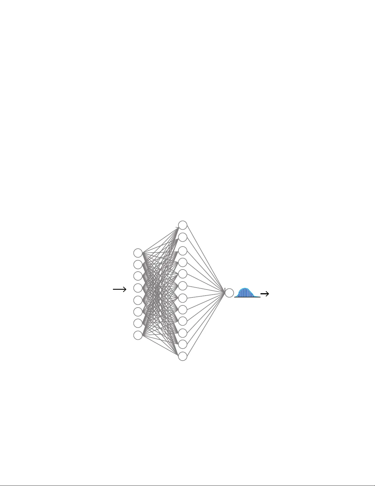
Original Paper
Loading high-quality paper...
Comments & Academic Discussion
Loading comments...
Leave a Comment