Bayesian test of normality versus a Dirichlet process mixture alternative

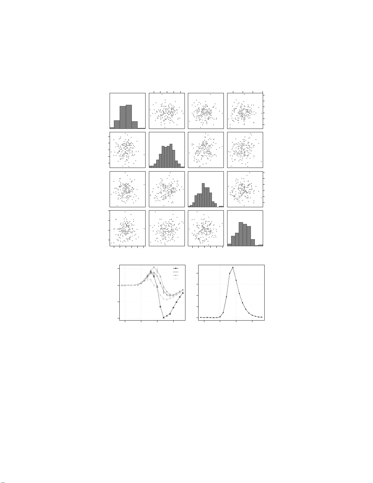
Bayesian test of normality v ersus a Dirichlet process mixture alternati ve Surya T . T okdar Department of Statistical Science, Duke University , Durham, North Carolina 27708, U.S.A. Ryan Martin Department of Statistics, North Carolina State University Raleigh, North Carolina 27607, U.S.A. November 15, 2 0 19 Abstract W e propose a Bay esian test of n ormality for uni v ariate or multi v ariate data a gainst alternati ve nonparametric models characterized by Dirichlet process mixture distributions. The alternativ e models are based on the principles of embedding and predictiv e matching. They can be inter- preted to offer rando m granulation of a normal distribution into a mixture of normals with mix- ture components o ccupy ing a smaller v olume the f arther they are from the distribution center . A scalar param etrization based on latent clustering is used to cover an entire spectrum of separation between the normal distr i butions and the alt ernati ve models. An efficient sequential i mportance sampler is dev eloped to calculate Bayes factors. S imulations indicate the proposed test can detect non-normality without fav oring the nonparametric alternativ e when normality holds. Ke y words: Bayes factor; embedding; goodness -of-fit; i mportance sampling; noninformativ e prior; predictive matching. 1 Introd uction Professor Jayanta K. Gho sh has left behind a lasting legacy in many areas of statistics research . Three prominen t such ar eas are ( a) fo rmal/objective Bayes, (b) no nparame tr ic mod els, and (c) model compa r ison/selection. One interesting pr o blem that lies at the intersection of these thre e areas is the question of form a lly assessing th e fit of a param etric model ag ainst non parametr ic a lter- natives (T okd ar et al., 2010). I n this paper we attemp t to settle this q uestion wh en assessing th e fit of univ ariate or mu ltivariate norm al mod els. Altho ugh sev eral good ness-of-fit tests exist for assess- ing no rmality with the usual emphasis on th e null mode l (Cardoso de Oliveira an d Ferreira, 2010; Aldor-Noiman et al., 2013; V oinov et al., 20 16), curr ently lack ing in the literature is a satisfactory formal Bayesian solu tion that also p lac es equal empha sis o n the altern ativ es, i.e., on th e possible modes of departu re fr o m no rmality . The av ailability of nonpar ametric alternativ es means para m etric models are no longe r indis- pensable. At the same time, when appro p riate, they p rovide co nsiderable simplification an d more penetrative inferen ce co mpared to a n onpar a m etric model. But it is im portant that the y are first tested for appro priateness. In some cases param etric models directly represent a p recise scientific 1 hypoth esis, suc h as the Gaussianity o f the Cosmic Micr owa ve Backgrou nd (e.g., Barreiro et al., 2007). In many o ther cases par ametric mod els provide the clearest mod eling f ramework to em b ed a scientific hyp othesis. For example, th e hyp othesis of flipping b etween stationary states by a neu ron in respon se to m ultiple stimuli ( Abeles et al. , 1995; Jon es et al., 20 0 7) is most easily tested when stationary states are describ ed b y identifiable param e tr ic mod els. When add itional d ata are av ailable from single stimulus trials, the p arametric model can be and sho uld b e te sted first. A f ormal Bayesian assessment of mode l fit is challengin g for sev eral re a sons. It requires a com - plete specificatio n of an alter n ativ e model and inv olves the difficult ca lculation of the Bayes factor: the ratio between the m arginal d ata likelihood scores un der the nu ll and alternative specification s. In assessing the fit of a param e tr ic mod el it is nearly imp ossible to specif y a broad alternative model without using subjective knowledge. But p rogre ss has been made in th is direc tio n with ad vances in non parametr ic Bay es method ology; see Berger and Gu glielmi (200 1); V erdinelli an d W asserman (1998); Flor e ns e t al. (1 996); Carota and Parmigiani (1 996). Th ese authors h av e advocated for a cer- tain level of form a lism in choosing a n onparam etric altern ativ e that is not only an attractive model for data analy sis, but can also be viewed as an extension of the n ull p arametric model that rema in s non-in formative with respe ct to the param eters of th e n ull model. In particular, Berger an d Guglielmi (200 1 ) advocate choosing a non parametr ic alternative tha t is balance d again st the parametric null in th e sense of emb e dding and predictive ma tching p roper- ties. Loosely spe a king, embedding r efers to the prop erty that the alternative mode l space can be partitioned in such a way that ea c h partitio n repr esents an unb iased relax ation of one an d o nly one element of the par ametric model space. Given such an emb edding , the same para meter θ that indexes the elemen ts of the null mo del could be used to index th e partition s of the alternative model, an d, a co mmon, no ninfor mative prio r may be used on θ u nder either specification. Pr e dictiv e matching formalizes this corresp o ndence in a stro ng tech nical way , demand ing that the Bayes factor remain neutral between the null and the alter native until one has accumulated sufficient amount of data. That “sufficient am ount” is taken to be the minimu m sample size needed to get pr oper po steriors on θ unde r bo th specification s. W ith this for m alism in mind , we p ursue a new Bayesian method fo r assessing th e fit of the n or- mal mo del to univ ariate o r mu lti variate data . Cur rently there ar e two fully developed a p proach es to- ward assessing the fit of the n ormal mo del, the Gau ssian pro cess app roach of V er dinelli an d W asserman (1998) and th e Polya tree approa c h of Berger and Guglielm i (2 001). W e pr opose a new a lter native model b ased on a Dirichlet process loca tio n-scale mix ture of no rmals (Lo, 1 984) with sev eral ad- vantages over these existing techniqu es. The Gau ssian process appr oach is difficult to com pute with and d oes n ot allow for embed ding and predictive m a tching. The P ´ olya tree ap proach is easy to work with for univariate data. But its re liance on partition -based co mputing d o es no t scale well with data dimensio n . Mo reover , a Polya tree distribution is a m odel for den sities tha t a re nowhere differentiable (Chou d huri et al., 2005). This may lead to inefficient estimation under the altern ativ e (van der V aart and van Zanten, 2008; Castillo, 20 08) which, in tur n, may lead to a sub-optim al de te c tio n of non -norm ality . Our simulation study provide s evidence suppor ting this claim. In con trast, o ur Dirichlet p r ocess mixtur e of n ormals model is in itself an attractive m odel for estimating a smo oth den sity . Dirich le t process mixture of no rmals have been we ll studied in the literature and are known to be easy to comp ute with, of ten via efficient Gib bs sampling o r its vari- ations ( Escobar and W est, 1 995; MacE achern an d M ¨ uller, 199 8; MacEach e rn, 19 98; Neal, 2 000), and a r e known also to p ossess op timal, ad aptive conv ergence rates in a variety of density estimation applications (Ghosal and van d er V aart, 200 1, 2 0 07; Sh en et al., 2013). In fo r mulating a Dirichlet process mix ture of no rmals, we diverge sligh tly from stand ard con- structions and use a normal- multivariate-beta base me asure (Section 2.2); see Griffin (2 010) fo r 2 a re la te d for m ulation. This helps u s con struct a collection of Dirichlet pr ocess m ixture of nor mals priors which are map ped o ne-to-o ne to th e co llection of all no rmal den sities. Eac h ele m ent of the alternative mo del may b e u nderstoo d as a rand om gran ulation of the cor respond ing n ormal d ensity into a mix ture of norm a ls with th e volume of a mixture com p onent negatively corr elated with its lateral shift from the center . Our alternative m odel is p arametrized by a single scalar par ameter, the pr ecision parame te r of the un derlying Dirichlet pro c ess. The prec ision par ameter controls the extent of g ranulation , i.e., latent clustering, which is key in determ ining the separatio n between th e null and the alternative. Other potential mo del par ameters, such th ose con tr olling the extent of lateral shifts of the mixture comp onents, are caref ully mappe d to the prec ision para meter to avoid identifiability problem s when precision is clo se to z e r o or infinity . Despite the slightly different fo rmulation , ou r Dir ic h let process mix ture of normals mod el is amenable to Gib bs samplin g fo r posterior comp utation and to sequential imputatio n (Liu, 1996) an d posterior ordin ate calcu la tio n (Basu an d Chib, 200 3) for Baye s factor co mputation . I n Section 3, we propo se a reaso nably efficient alg orithm fo r Bayes factor co mputation by adapting Liu’ s seque n tial imputation tech nique to our form ulation and augme nting it with impo rtance sampling to deal with additional par ameters that are not p art of the Dirich let proce ss m ixing distribution. This algo rithm is demo nstrated to per form much b etter than two reason able adap tations of the poster io r ord inate approa c h (Basu and Chib, 2003). For a nalyzing mu ltiv ariate da ta, we p r opose a n extension of th is algorithm th at uses a Rao –Blackwellized par a m eter augmen tation tec hnique, bor rowing ideas from sequential Monte Carlo. Section 5.1 p resents a simulation stu d y of the pro posed method ’ s T y pe I and II error proba b ilities within a freq uentist setting of hypo thesis testing . In a univ ariate setting, the resulting test is fo und to offer mod e rate to large improvements in power fo r a given size when compar e d to a test b ased on the P ´ olya tree app roach (Berger an d Gug lielmi, 2 001) and the classical Anderson –Darling test. In Section 5.2 we ad dress the importan t issue of Bayes factor consistency (T okd a r et al., 201 0) wh ic h refers to the desirable frequen tist pro perty: Bayes factor goes to ∞ un der the null and goes to 0 under the alter nativ e asympto tically as sample size grows to infinity . W e do no t con sider a full theoretical study of Bayes factor consistency , du e to severe techn ic a l challeng e s, but we provide a large sam ple simulatio n study with sample size up to 5000. Our simulations give stro ng evidence of consistency under the null. Co n sistency under th e a lter native is well expe c ted for Dirichlet process mixture models (T o k dar et al. , 2 010, Section 4). 2 A Dirichlet mixture of n ormals method for testing normality 2.1 Formalization of the testing pr oblem Consider data X 1: n = ( X 1 , . . . , X n ) wher e X i ∈ R p , i = 1 , . . . , n are mo d eled as n indepe n dent draws from an u nknown comm on pr obability distribution F . Le t F µ,σ denote a p -variate no rmal distribution with mean µ and covariance matrix σ σ ⊤ in Cholesky d e c omposition form and define F 0 = { F µ,σ : µ ∈ R p , σ ∈ T p } where T p is th e set o f all p × p lower-triangular matrices with positive diago nal elem ents. Our go al is to test H 0 : F ∈ F 0 . Unlike classical g oodne ss-of-fit tests, any Bayesian appro a ch to this testing pr oblem r e quires two additional mod e l ingre dients. First, the nu ll m odel requires a possibly impro per prio r distribution π 0 on R p × T p . Seco nd, an alternative mo del H 1 : F ∈ F 1 is req uired, alo ng w ith a prior Π 1 on F 1 . For a no n-subjective treatme n t, it is natur al to cho ose F 1 an infinite- d imensional subset of pr o bability measures on R p , and Π 1 a pr obability measure sup ported on F 1 . Once the priors π 0 and Π 1 are 3 specified, one can repo rt the Bayes factor B = R R p × T p  Q n i =1 dF µ,σ ( x i )  dπ 0 ( µ, σ ) R F 1  Q n i =1 dF ( x i )  d Π 1 ( F ) (1) as a measur e of e vidence ag ainst H 0 when X 1: n = x 1: n are o bserved. Small B indica tes th e parametric mo del p rovides an u nsatisfactory fit to the d ata. Refer to Kass and Raf ter y (1995) for more on the Bayes factor an d its inter pretation. 2.2 Local alternati ve, null embedd ing and a new Dirichlet pr ocess mixture For a non-sub jectiv e test, Berger an d Gug lielmi (2 0 01); V er dinelli an d W asserman ( 1998); Florens e t al. (1996) and Carota and Parmigia n i (19 9 6) stress o n the importan ce of main taining b alance b etween the n ull mod el and the no n-param etric altern a ti ve. All the se auth ors recomme n d specifying Π 1 as R Π µ,σ dπ 1 ( µ, σ ) a m ixture of local altern ativ es Π µ,σ mapped one -to-one to the elements F µ,σ of th e null m odel. Mo st of these autho rs require th is mappin g to be given by embedd ing the null element as the mean of th e lo cal a lter native: R F d Π µ,σ ( F ) = F µ,σ for every ( µ, σ ) . This is difficult to achieve with the comm only used Dirich let p rocess mixture of norm als (E sco bar and W est, 199 5) that use a normal- inverse-W ishart base measur e. W e offer the fo llowing mo dification alon g the lines of Griffin (2010). Let S p be the spa ce of p × p symm e tr ic positive defin ite matrices with all p eigenv alues in (0 , 1) . For scalars ω 1 and ω 2 greater than ( p − 1 ) / 2 , let Be ( ω 1 , ω 2 ) deno te the multiv ariate b eta d istribution on S p (Muirhead, 2005, Chap. 3.3 ) having density Be ( v | ω 1 , ω 2 ) = a p ( ω 1 , ω 2 )(det v ) ω 1 − ( p +1) / 2 { det( I p − v ) } ω 2 − ( p +1) / 2 , (2) where I p is the p × p iden tity matrix and a p ( ω 1 , ω 2 ) = Γ p ( ω 1 + ω 2 ) / Γ p ( ω 1 )Γ p ( ω 2 ) , with Γ p the p - variate gamma fu nction. Write Ψ fo r the prob ability measur e on R p × S p giv en by the law of ( U, V ) , where V ∼ Be ( ω 1 , ω 2 ) and U | V ∼ N (0 , I p − V ) . Th is law is well-defin ed, since I p − V ∈ S p with probab ility 1. Let DP ( α, Ψ) de n ote th e Dirich le t pro cess d istribution with precision α > 0 and ba se m easure Ψ from above (Ferguson, 197 3). Recall th at ¯ Ψ ∼ DP ( α, Ψ ) means th at f o r any positive in teger k and any measurab le p artition B 1 , . . . , B k of R p × S p , the prob ability vector { ¯ Ψ( B 1 ) , . . . , ¯ Ψ( B k ) } h as a k -d imensional Dirichlet distribution with parameter s { α Ψ( B 1 ) , . . . , α Ψ ( B k ) } . For any ( µ, σ ) , let DPM µ,σ ( α, Ψ) d enote th e distribution of the ra n dom pr obability measure ¯ F µ,σ = Z N ( µ + σ u, σ v σ ⊤ ) d ¯ Ψ( u, v ) , where ¯ Ψ ∼ DP ( α, Ψ); (3) then we have the following r e sult. Theorem 1. F or an y ( µ, σ ) a nd a ny α , the mean of DPM µ,σ ( α, Ψ) is N ( µ, σ σ ⊤ ) . Pr oof. For an ¯ F µ,σ as in (3), its expecta tio n is simply R N ( µ + σ u, σ v σ ⊤ ) d Ψ( u, v ) = R { R N ( µ + σ u, σ v σ ⊤ ) d N ( u | 0 , I p − v ) } d Be ( v | ω 1 , ω 2 ) by defin ition of Ψ . But the inner integral always equals N ( µ, σ σ ⊤ ) by the well-k n own Gaussian co nvolution id e ntity . W e cho ose DPM µ,σ ( α, Ψ) as the local alternative Π µ,σ to F µ,σ , with T heorem 1 en suring local embedd in g. I t is mo re conv enient to write our nu ll an d alternative models in the fo llowing hierar- chical manner . H 0 : X 1: n | ( µ, σ ) iid ∼ F µ,σ , ( µ, σ ) ∼ π 0 (4) H 1 : X 1: n | ( ¯ F µ,σ , µ, σ ) iid ∼ ¯ F µ,σ , ¯ F µ,σ | ( µ, σ ) ∼ DPM µ,σ ( α, Ψ) , ( µ, σ ) ∼ π 1 ; (5) 4 The choice of π 0 , π 1 will be discussed in Section 2 .5. 2.3 Understanding local alternativ e as a random granulation For any space S and an s ∈ S , let h s i d e n ote th e degenera te p robab ility distribution o n S with po int mass at s . Due to the stick-break ing rep r esentation o f a Dirichlet p rocess (Sethur aman, 1 994) a random ¯ Ψ ∼ D P ( α, Ψ ) can be written as ¯ Ψ = X h ≥ 1 q h h ( U h , V h ) i , (6) where ( U h , V h ) , h ≥ 1 , are indepe n dently draws fro m Ψ , q h = β h Q j p − 1 and any Ψ ∈ S p , let W ( ν, Ψ) an d IW ( ν, Ψ ) deno te, respectively , th e Wishart and the inv erse-W ishart distributions with shap e ν and scale Ψ . The null po sterior density , viewed throug h the ( µ, Σ) param etrization, co uld b e c on veniently written as: f H 0 ( µ, Σ | x 1: n ) = IW (Σ | n − 1 , ( n − 1) S ) × N ( µ | ¯ x, n − 1 Σ) . W e take f µ,σ imp ( µ, σ ) to be a heavy tailed a pprox imation to it, contro lled b y two scalar parameter s ν > p − 1 , ρ > 0 , and g i ven by: f µ, Σ imp ( µ, Σ) = F (Σ | ν − ( p − 1) , ν , S ) × t ν ( µ | ¯ x, ρ Σ / n ) where F ( κ, δ, Ψ) deno tes the ma trix F d istribution (Mu lder an d Pericchi, 2018) with shapes κ > 0 , δ > p − 1 and scale Ψ ∈ S p . Under this im p ortance de n sity one cou ld write Σ | Φ ∼ IW ( ν, Φ) , Φ ∼ W ( ν , S ) . See Ap pendix B for mor e details on efficient rando m sampling and probability density ev aluation of such a Σ . In our n umerical experiments, we used ν = max { p + 1 , n − p √ n } and ρ = √ n ; but the results were not too sen siti ve to these choices. 3.3 Comparison with Basu and Chib (2003) The likeliho od-po sterior or d inate recip e of Chib (199 5) appro ximates f H 1 ( x 1: n ) b y th e quantity π L ( µ ⋆ , σ ⋆ ) f H 1 ( x 1: n | µ ⋆ , σ ⋆ ) /f H 1 ( µ ⋆ , σ ⋆ | x 1: n ) wher e ( µ ⋆ , σ ⋆ ) is any point of high posterio r den- sity . T o appro x imate the likelihood ord inate f H 1 ( x 1: n | µ ⋆ , σ ⋆ ) once a ( µ ⋆ , σ ⋆ ) h as been chosen, Basu and Chib (2 003) r ecommen d using the im portance sam pling scheme on ( S 1: n , V ) describ ed in Section 3.1 conditio nal on µ = µ ⋆ , σ = σ ⋆ , leading to the fo llowing approx imation to B b B − 1 = f H 0 ( µ ⋆ , σ ⋆ | x 1: n ) f H 1 ( µ ⋆ , σ ⋆ | x 1: n ) 1 M M X m =1 n − 1 Y i =0    α α + i + λ m i X ℓ =1 k m ℓ ( i ) α + i N ( x i +1 | µ m ℓ , σ m ℓ σ m ⊤ ℓ ) N ( x i +1 | µ ⋆ , σ ⋆ σ ⋆ ⊤ )    (17) Basu and Chib (20 03) recomm end identify ing ( µ ⋆ , σ ⋆ ) b y r unning an initial Markov chain sam- pler , preferab ly a Gib bs sampler which can also p rovide a Rao–Blackwellized Mon te Carlo ap - proxim a tion to the posterior or d inate f H 1 ( µ ⋆ , σ ⋆ | x 1: n ) . Altern ativ ely o ne cou ld g a th er p osterior samples of ( µ, σ ) and use efficient smoo thing b ased density estimation techn iques to approx imate f H 1 ( µ ⋆ , σ ⋆ | x 1: n ) . W e follow both su ggestions to con struct two co mpetitors of our im portance sam - pling algorithm for the u niv ariate c ase. T able 1 gives summaries o f 100 replication s of the Bayes factor comp u tation on a single syn- thetic data set we simulated with 100 draws from the standar d no rmal den sity . “Basu–Ch ib” refers to Monte Carlo po sterior ordin ate appro ximation based on a Gib bs sampler, which is fairly straight- forward to design fo r our cho ic e of Dirich let process mixture (see e.g., Escob a r and W est , 1995, for a basic construction ). “Basu–Chib + smoothing” refers to posterior ord inate appr oximation based o n kernel smoothing of the Gibb s sampler draws of ( µ, σ ) . Smoothin g was don e by the kde function of the R -p ackage ks , with bandwid th chosen by the plug-in meth od of W and an d Jones 11 Algorithm Mean Min. 1st Q. Median 3rd Q. Max Time Basu–Chib 1.66 0.000 5 0.86 1.61 2.32 7.7 3.6s Basu–Chib + smoo thing 1.82 1.39 1 .68 1.79 1.92 2.95 3.7s Impor tan ce sampling 1 .82 1.54 1 . 76 1.81 1.87 2.03 0.8s T able 1: Compariso n of our impo rtance samp lin g me th od a gainst two versions of the Basu an d Chib (2003) alg o rithm; see text for more details. Columns 2 th rough 7 g ive sum maries o f 10 0 rep lications of th e Bay es factor comp utation on the same data set of 1 00 draws from the standard normal density . Last colum n refe r s to r u n time in seconds per comp utation. (1994). W e also tried th e more co mputation ally expen si ve cross-validation cho ice of the band width (Duong and Hazelton, 2 005) which d id n ot result in any appreciab le imp rovement in perfor mance (not repo rted). “ I mportan ce samplin g” ref ers to o ur appr oach. E ach algorithm was ru n with 10,00 0 importan ce samples. “Basu– Chib” alg orithm r equired two add itio nal run s o f the Gibb s sampler, one to id entify µ ⋆ , σ ⋆ as median d raws and th e other to ap proxim ate the po sterior o rdinate. “ Basu– Chib + smoothing ” requ ires o n ly o ne run o f the Gibb s sampler to simultaneou sly identify µ ⋆ , σ ⋆ and g ather p osterior draws of µ, σ to b e used in smoo thing. All ru ns of Gibb s sampler were 10 ,000 iterations each. T able 1 m akes it clear that our im p ortance sampling a p proach o ffers a mo re efficient estima- tion of the Bayes factor with sub stantially lower co mputing cost than either Basu–Chib alg orithm. The po ster ior ordinate appro x imation step appear s suspect f or the p oor perf o rmance of the latter . Smoothing helps, but not to the exten t to m ake th e likelihood-p o sterior ordinate metho d co m petitive against our importa n ce sampling algorith m. 3.4 Additional considerations f or multivariate data A weak ness of the impo rtance sam p ling scheme described above is that th e sampling of the atoms V 1: n does no t incorp orate any in formatio n from th e data. Each time an ob ser vation is assign ed to a new cluster ℓ , the clu ster’ s variance comp onent V ℓ is sampled f r om the prior and never updated . This could be particularly troubleso m e in higher dimension s where the chan ces of rand omly land ing on an ap propr iate V ℓ for eac h n ew c luster are very slim. As a po ssible mitigation of th is sampling inefficiency , we propo se a Rao -Blackwellization extension inspir ed by sequential Monte Carlo id eas where each V ℓ is r epresented by a set of particles V ⋆ ℓr , r = 1 , . . . , R , whose weights are up dated ev ery tim e a new ob servation is ad ded to the ℓ -th cluster . T o be more pre c ise, notice that the samplin g of V 1: n under the altern ativ e prior cou ld b e repr e- sented as: for eac h i = 1 , . . . , n , sample V ⋆ ir ∼ Be ( ω 1 , ω 2 ) , r = 1 , . . . , R , ind ependen tly o f each other, and then set V i to b e one o f the V ⋆ ir chosen at random . W ith V ⋆ = V ⋆ 1: n, 1: R , on e ca n th en integrate V 1: n from the mo del an d rewrite ( 12) and (13) as f X i +1 ( x i +1 | x 1: i , s 1: i , v ⋆ , µ, σ ) = α α + i N ( x i +1 | µ, σ σ ⊤ ) + λ i X ℓ =1 k ℓ ( i ) α + i R X r =1 q ℓr ( i ) N ( x i +1 | µ ℓr , σ ℓr σ ⊤ ℓr ) , (18) f S i +1 ( ℓ | x 1:( i +1) , s 1: i , v ⋆ , µ, σ ) = ( c − 1 k ℓ ( i ) P R r =1 q ℓr ( i ) N ( x i +1 | µ ℓr , σ ℓr σ ⊤ ℓr ) , ℓ = 1 , . . . , λ i c − 1 α N ( x i +1 | µ, σ σ ⊤ ) , ℓ = λ i + 1 , (19) 12 where µ ℓr and σ ℓr are comp u ted as in (1 4) but with v ⋆ ℓr instead o f v ℓ , and , q ℓr ( i ) = m ℓr ( i ) / { m ℓ, 1 ( i )+ · · · + m ℓ,R ( i ) } , r = 1 , . . . , R , with m ℓr ( i ) = exp[ − k ℓ ( i )tr { S ℓ ( i )( σ v ⋆ ℓr σ ⊤ ) − 1 } ] det( v ⋆ ℓr ) k ℓ ( i ) − 1 2 N  ¯ x ℓ ( i ) | µ, σ { v ⋆ ℓr /k ℓ ( i ) + I p − v ⋆ ℓr } σ ⊤  , where ¯ x ℓ ( i ) = k ℓ ( i ) − 1 P j ≤ i x j I ( s j = ℓ ) is th e cu r rent cluster mean and S ℓ ( i ) = k ℓ ( i ) − 1 P j ≤ i ( x j − ¯ x ℓ ( i ))( x j − ¯ x ℓ ( i )) ⊤ I ( s j = ℓ ) is the curren t cluster variance when only the first i observations have been pro cessed. The co rrespon ding impor tance sampling density for ( S 1: n , V ⋆ , µ, σ ) is defined analogo usly with V replaced by V ⋆ . Th e calculation of th e im portance weights is mo dified acc o rdingly . Maintainin g and updatin g th e r e lati ve weights of the R p articles fo r each cluster par a meter V ℓ offers a greater incorpo ration of the observed d a ta . W e expect a larger R to b e n eeded for high e r d imension, as the space o f V matrices is p ( p + 1 ) / 2 dimensiona l. W e suggest a d e fault cho ice of R = p ( p + 1) , although a thorou gh investigation of this choice is beyond the scope o f this pap er . The num erical experiments repo rted in th e next sectio n were carried out with this d efault choice . 4 Case studies Example 4.1 . Berger and Gu glielmi (2 001) illustrate their Polya tree test on the lo g -lifetime mea- surements of 1 00 Ke vlar pressure vessels (Andrews and Herzb erg , 19 85, p. 183) . Our altern ativ e model produ ces a min imum Bayes factor clo se to 10 − 5 for α ∈ [2 − 6 , 2 13 ] , sh owing negligible evi- dence toward normality . W e used 2 0,000 impor tance samples to com pute ˆ B . Our minimu m Bayes factor is similar in magnitu de to the o n e reported by Berger an d Guglielmi (2001). Example 4.2. Figure 2 shows scatterp lots of three synthetic datasets of size n = 1 0 0 an d dim ension p = 2 simu lated respe cti vely from a b iv ariate standard norma l, a biv ariate standar d Studen t-t with three degrees of fre edom, and a Frank copula distribution (par ameter = 20 which co rrespond s to Kendall’ s τ = 0 . 816 ) with standard norma l m arginals. For each data set, the Bayes factor was calculated over a regu lar grid o f α ∈ [2 − 6 , 2 13 ] with 10 ,000 importa n ce samples. Each calculation was replicated 8 indepe n dent times to assess rep roduc ib ility . W e report in Figu re 2 the med ia n , minimum an d maxim u m of these 8 lo g Bayes factor ev aluations, alon g with a c ombined estimate obtained by p ooling the 8 × 1 0 , 000 imp ortance sample s together . The gra phs inde ed sugg est that these calculations were fairly rep roducib le. For the first dataset the Bayes factor remain s essentially larger th an 1 for all p recision p a r am- eter values and b ecomes quite large for mod erate α , in dicating little dou bt again st no rmality . T he Student-t d ataset shows a con c entration o f poin ts ar ound (0 , 0 ) along with a numb e r o f outliers, suggesting a heavier-than-normal ta il. The Bayes factor bottoms out around 1 0 − 12 with fairly small values in the ran ge 0 . 5 ≤ α ≤ 8 wher e the prior encou rages a m oderate numbe r o f clusters. Pre- sumably , the alternative is able to pick up th e h eavy tail by assignin g the large ou tliers in to separate clusters. For the co pula dataset with a non- e lliptical scatter, the Bayes factor achiev es a minimum of 10 − 7 suggesting stron g evidence ag ainst n ormality . In terestingly , the Bayes factor dips b elow 1 across two distinct segments of α values: α ≤ 8 and α ≥ 2 11 . The la tter segmen t co rrespon ds to, a priori , a large num ber o f mix ture comp onents where e ach co mponen t has a tiny volume shar e (refe r to Figure 1). Example 4 .3. The well known Eg yptian skulls dataset (Hand et al., 1994) consists o f p = 4 m ea- surements (MB: m aximal br eadth, BH: basibr egmatic h eight, BL: basialveolar leng th, and , NH: 13 ● ● ● ● ● ● ● ● ● ● ● ● ● ● ● ● ● ● ● ● ● ● ● ● ● ● ● ● ● ● ● ● ● ● ● ● ● ● ● ● ● ● ● ● ● ● ● ● ● ● ● ● ● ● ● ● ● ● ● ● ● ● ● ● ● ● ● ● ● ● ● ● ● ● ● ● ● ● ● ● ● ● ● ● ● ● ● ● ● ● ● ● ● ● ● ● ● ● ● ● − 2 − 1 0 1 2 − 2 − 1 0 1 2 x 1 x 2 ● ● ● ● ● ● ● ● ● ● ● ● ● ● ● ● ● ● ● ● ● ● ● ● ● ● ● ● ● ● ● ● ● ● ● ● ● ● ● ● ● ● ● ● ● ● ● ● ● ● ● ● ● ● ● ● ● ● ● ● ● ● ● ● ● ● ● ● ● ● ● ● ● ● ● ● ● ● ● ● ● ● ● ● ● ● ● ● ● ● ● ● ● ● ● ● ● ● ● ● − 4 − 2 0 2 4 6 − 4 − 2 0 2 4 6 8 x 1 x 2 ● ● ● ● ● ● ● ● ● ● ● ● ● ● ● ● ● ● ● ● ● ● ● ● ● ● ● ● ● ● ● ● ● ● ● ● ● ● ● ● ● ● ● ● ● ● ● ● ● ● ● ● ● ● ● ● ● ● ● ● ● ● ● ● ● ● ● ● ● ● ● ● ● ● ● ● ● ● ● ● ● ● ● ● ● ● ● ● ● ● ● ● ● ● ● ● ● ● ● ● − 2 − 1 0 1 2 − 3 − 2 − 1 0 1 2 x 1 x 2 − 5 0 5 10 0 5 10 15 log 2 ( α ) log 10 ( BF ) ● ● ● ● ● ● ● ● ● ● ● ● ● ● ● ● ● ● ● ● − 5 0 5 10 − 15 − 10 − 5 0 5 10 log 2 ( α ) log 10 ( BF ) ● ● ● ● ● ● ● ● ● ● ● ● ● ● ● ● ● ● ● ● − 5 0 5 10 − 5 0 5 10 log 2 ( α ) log 10 ( BF ) ● ● ● ● ● ● ● ● ● ● ● ● ● ● ● ● ● ● ● ● Figure 2 : Bayes factors (top) f or data (b ottom) in Exam ple 4.2; n o rmal (lef t), Student-t (mid dle), Frank co pula with Gaussian marginals (righ t). For each dataset, Bay es factors were calculated for precision param eter α = 2 k with an integer k r unning from − 6 thr ough 13. Each Bayes factor calculation was r epeated 8 times with 10, 000 imp o rtance samples each. T h e median, minimu m and maximum Bayes factor values ( in base 10 lo garithm) are shown as a vertical segmen t superim p osed with a filled circle. The dashed lin e shows a com bined estima te of the Baye s factor by poolin g together all the 8 × 1 0 , 000 importan ce sample draws. nasal heigh t, all in mm) taken on n = 150 an cient Egyptian skulls f rom five time epochs dur ing 4000 B.C. and 20 0 A . D. Mea n effect of time was removed by r u nning a multivariate analy sis of variance, an d we test the residuals for norm ality . Ties were bro ken by injecting a small jitter to each ob servation with rand om un iform draws betwe e n [ − 1 / 60 , 1 / 60] . A chi- square QQ-plo t (not shown) o f the Mahalanobis distance squares showed a faint deviation fr o m n ormality . Mard ia’ s ske wness an d kurto sis tests failed to reject n ormality with p-values ≈ 0 . 5 . Interestingly , ou r app r oach showed moder ately strong evidence against n ormality wh en the fo ur measuremen ts were analyzed separately , but little evidence against no rmality f or their joint distri- bution (Figure 3). This situation is very different fr om the co pula exam ple con sidered above, wher e marginal distributions were norm a l but non- normality co uld be detected f or the joint distribution. A po tential explanatio n is that given the pr edictive m atching pro perty of our appro a ch, it will take more observations in 4 d imensions to d e tect n on-no rmality than in a un iv ariate case. For example, if we had only 5 o bservations fro m a 4 dimen sio nal d istribution, o ur appr oach is g uaranteed to prod uce a Bayes factor of 1 in the joint analysis, but m ay be able to de tec t non- normality o f the m arginals. Howe ver , this does not fully explain the stark difference between the univariate and the multivariate results r eported in Figure 3. It is possible that the joint distribution deviates fr om n ormality in ways that a r e not well cap tured by the mix ture alternative p roposed here, whereas u niv ariate p rojections are well appr oximated as mix tures of n ormals. 14 MB − 10 − 5 0 5 10 ● ● ● ● ● ● ● ● ● ● ● ● ● ● ● ● ● ● ● ● ● ● ● ● ● ● ● ● ● ● ● ● ● ● ● ● ● ● ● ● ● ● ● ● ● ● ● ● ● ● ● ● ● ● ● ● ● ● ● ● ● ● ● ● ● ● ● ● ● ● ● ● ● ● ● ● ● ● ● ● ● ● ● ● ● ● ● ● ● ● ● ● ● ● ● ● ● ● ● ● ● ● ● ● ● ● ● ● ● ● ● ● ● ● ● ● ● ● ● ● ● ● ● ● ● ● ● ● ● ● ● ● ● ● ● ● ● ● ● ● ● ● ● ● ● ● ● ● ● ● ● ● ● ● ● ● ● ● ● ● ● ● ● ● ● ● ● ● ● ● ● ● ● ● ● ● ● ● ● ● ● ● ● ● ● ● ● ● ● ● ● ● ● ● ● ● ● ● ● ● ● ● ● ● ● ● ● ● ● ● ● ● ● ● ● ● ● ● ● ● ● ● ● ● ● ● ● ● ● ● ● ● ● ● ● ● ● ● ● ● ● ● ● ● ● ● ● ● ● ● ● ● ● ● ● ● ● ● ● ● ● ● ● ● ● ● ● ● ● ● ● ● ● ● ● ● ● ● ● ● ● ● ● ● ● ● ● ● ● ● ● ● ● ● ● ● ● ● ● ● − 5 0 5 10 − 10 0 5 10 15 ● ● ● ● ● ● ● ● ● ● ● ● ● ● ● ● ● ● ● ● ● ● ● ● ● ● ● ● ● ● ● ● ● ● ● ● ● ● ● ● ● ● ● ● ● ● ● ● ● ● ● ● ● ● ● ● ● ● ● ● ● ● ● ● ● ● ● ● ● ● ● ● ● ● ● ● ● ● ● ● ● ● ● ● ● ● ● ● ● ● ● ● ● ● ● ● ● ● ● ● ● ● ● ● ● ● ● ● ● ● ● ● ● ● ● ● ● ● ● ● ● ● ● ● ● ● ● ● ● ● ● ● ● ● ● ● ● ● ● ● ● ● ● ● ● ● ● ● ● ● − 10 − 5 0 5 10 ● ● ● ● ● ● ● ● ● ● ● ● ● ● ● ● ● ● ● ● ● ● ● ● ● ● ● ● ● ● ● ● ● ● ● ● ● ● ● ● ● ● ● ● ● ● ● ● ● ● ● ● ● ● ● ● ● ● ● ● ● ● ● ● ● ● ● ● ● ● ● ● ● ● ● ● ● ● ● ● ● ● ● ● ● ● ● ● ● ● ● ● ● ● ● ● ● ● ● ● ● ● ● ● ● ● ● ● ● ● ● ● ● ● ● ● ● ● ● ● ● ● ● ● ● ● ● ● ● ● ● ● ● ● ● ● ● ● ● ● ● ● ● ● ● ● ● ● ● ● BH ● ● ● ● ● ● ● ● ● ● ● ● ● ● ● ● ● ● ● ● ● ● ● ● ● ● ● ● ● ● ● ● ● ● ● ● ● ● ● ● ● ● ● ● ● ● ● ● ● ● ● ● ● ● ● ● ● ● ● ● ● ● ● ● ● ● ● ● ● ● ● ● ● ● ● ● ● ● ● ● ● ● ● ● ● ● ● ● ● ● ● ● ● ● ● ● ● ● ● ● ● ● ● ● ● ● ● ● ● ● ● ● ● ● ● ● ● ● ● ● ● ● ● ● ● ● ● ● ● ● ● ● ● ● ● ● ● ● ● ● ● ● ● ● ● ● ● ● ● ● ● ● ● ● ● ● ● ● ● ● ● ● ● ● ● ● ● ● ● ● ● ● ● ● ● ● ● ● ● ● ● ● ● ● ● ● ● ● ● ● ● ● ● ● ● ● ● ● ● ● ● ● ● ● ● ● ● ● ● ● ● ● ● ● ● ● ● ● ● ● ● ● ● ● ● ● ● ● ● ● ● ● ● ● ● ● ● ● ● ● ● ● ● ● ● ● ● ● ● ● ● ● ● ● ● ● ● ● ● ● ● ● ● ● ● ● ● ● ● ● ● ● ● ● ● ● ● ● ● ● ● ● ● ● ● ● ● ● ● ● ● ● ● ● ● ● ● ● ● ● ● ● ● ● ● ● ● ● ● ● ● ● ● ● ● ● ● ● ● ● ● ● ● ● ● ● ● ● ● ● ● ● ● ● ● ● ● ● ● ● ● ● ● ● ● ● ● ● ● ● ● ● ● ● ● ● ● ● ● ● ● ● ● ● ● ● ● ● ● ● ● ● ● ● ● ● ● ● ● ● ● ● ● ● ● ● ● ● ● ● ● ● ● ● ● ● ● ● ● ● ● ● ● ● ● ● ● ● ● ● ● ● ● ● ● ● ● ● ● ● ● ● ● ● ● ● ● ● ● ● ● ● ● ● ● ● ● ● ● ● ● ● ● ● ● ● ● ● ● ● ● ● ● ● ● ● ● ● ● ● ● ● ● ● ● ● ● ● ● ● ● ● ● ● ● ● ● ● ● ● ● ● ● ● ● ● ● ● ● ● ● ● ● ● ● ● ● ● ● ● ● ● ● ● ● ● ● ● ● ● ● ● ● ● ● ● ● ● ● ● ● ● ● ● ● ● ● ● ● ● ● ● ● ● ● ● ● ● ● ● ● ● ● ● ● ● ● ● ● ● ● ● ● ● ● ● ● ● ● ● ● ● ● ● ● ● ● ● ● ● ● ● ● ● ● ● ● ● ● ● ● ● ● ● ● ● ● ● ● ● ● ● ● ● ● ● ● ● ● ● BL − 10 0 5 10 15 ● ● ● ● ● ● ● ● ● ● ● ● ● ● ● ● ● ● ● ● ● ● ● ● ● ● ● ● ● ● ● ● ● ● ● ● ● ● ● ● ● ● ● ● ● ● ● ● ● ● ● ● ● ● ● ● ● ● ● ● ● ● ● ● ● ● ● ● ● ● ● ● ● ● ● ● ● ● ● ● ● ● ● ● ● ● ● ● ● ● ● ● ● ● ● ● ● ● ● ● ● ● ● ● ● ● ● ● ● ● ● ● ● ● ● ● ● ● ● ● ● ● ● ● ● ● ● ● ● ● ● ● ● ● ● ● ● ● ● ● ● ● ● ● ● ● ● ● ● ● − 10 0 5 10 15 − 5 0 5 10 ● ● ● ● ● ● ● ● ● ● ● ● ● ● ● ● ● ● ● ● ● ● ● ● ● ● ● ● ● ● ● ● ● ● ● ● ● ● ● ● ● ● ● ● ● ● ● ● ● ● ● ● ● ● ● ● ● ● ● ● ● ● ● ● ● ● ● ● ● ● ● ● ● ● ● ● ● ● ● ● ● ● ● ● ● ● ● ● ● ● ● ● ● ● ● ● ● ● ● ● ● ● ● ● ● ● ● ● ● ● ● ● ● ● ● ● ● ● ● ● ● ● ● ● ● ● ● ● ● ● ● ● ● ● ● ● ● ● ● ● ● ● ● ● ● ● ● ● ● ● ● ● ● ● ● ● ● ● ● ● ● ● ● ● ● ● ● ● ● ● ● ● ● ● ● ● ● ● ● ● ● ● ● ● ● ● ● ● ● ● ● ● ● ● ● ● ● ● ● ● ● ● ● ● ● ● ● ● ● ● ● ● ● ● ● ● ● ● ● ● ● ● ● ● ● ● ● ● ● ● ● ● ● ● ● ● ● ● ● ● ● ● ● ● ● ● ● ● ● ● ● ● ● ● ● ● ● ● ● ● ● ● ● ● ● ● ● ● ● ● ● ● ● ● ● ● ● ● ● ● ● ● ● ● ● ● ● ● ● ● ● ● ● ● ● ● ● ● ● ● − 10 0 5 10 15 ● ● ● ● ● ● ● ● ● ● ● ● ● ● ● ● ● ● ● ● ● ● ● ● ● ● ● ● ● ● ● ● ● ● ● ● ● ● ● ● ● ● ● ● ● ● ● ● ● ● ● ● ● ● ● ● ● ● ● ● ● ● ● ● ● ● ● ● ● ● ● ● ● ● ● ● ● ● ● ● ● ● ● ● ● ● ● ● ● ● ● ● ● ● ● ● ● ● ● ● ● ● ● ● ● ● ● ● ● ● ● ● ● ● ● ● ● ● ● ● ● ● ● ● ● ● ● ● ● ● ● ● ● ● ● ● ● ● ● ● ● ● ● ● ● ● ● ● ● ● NH (a) Data scatte r and histograms − 5 0 5 10 − 10 − 5 0 5 ● ● ● ● ● ● ● ● ● ● ● ● ● ● ● ● ● ● ● ● log 2 ( α ) log 10 ( BF ) ● x1 x2 x3 x4 (b) Indi vidual tests of normality − 5 0 5 10 0 50 100 150 200 log 2 ( α ) log 10 ( BF ) ● ● ● ● ● ● ● ● ● ● ● ● ● ● ● ● ● ● ● ● (c) Joint test of normality Figure 3 : Egyptian sk ull d ata a n alysis. For the single variable analy ses, each Bayes factor ev alua- tion was p erform e d using 1 0,000 impor tance samp les and r epeated 8 tim es. V ertical segments an d filled shapes show th e minimu m, maximu m and the m edian of the log Bayes factor values. A com- bined ev aluation of the same, obtained b y p ooling all 8 0,000 samples tog ether, is rep o rted via the dashed line. Same ev aluation stra tegy was adop ted for th e join t an alysis, but h ere each ev aluation was d one u sing 50,0 0 0 impor tance samples. 15 0.0 0.2 0.4 0.6 0.8 1.0 0.0 0.2 0.4 0.6 0.8 1.0 False P ositiv e Rate T r ue Positiv e Rate (a) Student-t, degre es of freedom 3 0.0 0.2 0.4 0.6 0.8 1.0 0.0 0.2 0.4 0.6 0.8 1.0 False P ositiv e Rate T r ue Positiv e Rate (b) Ske w-normal, s hape = 10 0.0 0.2 0.4 0.6 0.8 1.0 0.0 0.2 0.4 0.6 0.8 1.0 False P ositiv e Rate T r ue Positiv e Rate (c) Uniform on ( − 1 , 1) Figure 4 : Power -size cu rves for Dirichlet process mixtu r e (solid, black) , Po ly a tree (br oken, blac k ) and And e r son–Darlin g (solid, gray ) tests. Each pa nel p r esents power for a specific alternative bench- marked ag ainst size u nder the null hyp othesis of Gau ssianity . 5 Numerical experiments 5.1 Po wer -size comparison against P olya tr ee and Anderson–Darling Comparing the minimu m Baye s factor against a thresho ld gives a go odness-of -fit test o f norm a lity in the classical sense, subject to size and power calculation s. Size may be app roximated by simulating data from the null. Due to Lemm a 6, it is sufficient to simulate under any one nor mal distribution because of the loca tio n-scale inv ariance natu re of o ur alternative specification . W e r a n a simu lation study to comp a re size an d p ower of the resulting tests to tests deriv ed similarly fro m the Polya tree ap proach of Berger and Gu glielmi (20 01) and th e classical Anderson -Darling tests. For o ur approa c h , minim u m Bayes factor was calculated over α ∈ [2 − 6 , 2 4 ] . For the Poly a tree tests, we used th e fixed- partition ( T ype 2) version (Berger an d Guglielmi, 20 01, Eq u ation 2) with the functio n d ( ε m ) = h − 1 4 m for scale param e ter and calculated minim u m Bayes factor over h ∈ [2 − 6 , 2 4 ] . Size calculations were done with 10 0 datasets each co nsisting o f n = 10 0 draws fr o m th e standard no rmal d istribution. For power calculation under the alter native, we con sid e red th r ee non - normal distributions: Student-t with 3 d egrees of fr eedom, ske w-nor mal with shap e p arameter 10, and u n iform on th e interval ( − 1 , 1) . For any of these three distributions, power was ap proxima ted by simulatin g 100 datasets each with n = 100 d raws fr om the distribution. Results ar e shown in Figure 4 as p ower -size cu rves for th r ee sets of tests for each of th e c hosen non -norm al distributions. For all three distributions, the Dirich le t pro cess mixtu re tests perfo rm the best, prod ucing high e r power at a lower smaller size. An derson– D a r ling tests ge n erally outperf orm the Polya tre e tests. The results for the un iform distribution were surpr ising to us as we expected the Polya- tree alternative to beat Dirichlet pro c ess mix tu res at d etecting discontinuities. 5.2 Bayes factor consistency A desira b le frequ entist p r operty of a Bayesian testing pr ocedur e is Bayes factor con sistency , i. e., the Bayes factor sh o uld converge to ∞ asymptotically u nder the nu ll, a n d to 0 un der th e alternative as sample size grows to infinity . I t follows f r om a simple a rgu ment (e.g. T o k dar e t al., 20 10, Sec- tion 4) that B → ∞ almost surely wh enever X i ’ s are drawn f rom a non -norm al distribution that is in the Kullbac k –Leibler supp ort of the alter nativ e p rior distribution (Gho sh and Ramam oorthi, 16 0 1000 2000 3000 4000 5000 0 5 10 15 n Bay es factor Figure 5: Bayes factor sample path s, with 2 .5%, 50 %, and 97. 5 % sum m aries, when 10 0 datasets were gener a ted from a stan d ard normal d istribution. Each path represents one dataset, d epicting as a function of n ∈ N , th e Bayes facto r values calculated based on the first n obser vations in the dataset. About half of the sample p aths a re shown to impr ove clarity . 2003). Substantial existing litera tu re (Ghosal et al., 1 999; T okd ar, 20 06; Ghosal and van d er V aart, 2007; Shen et a l., 2013) ind icates th at Dirichlet pr ocess mixtures of normals prior d istributions have broad Kullback–Leib ler sup p ort wh ich can be character ized by mild con tinuity an d tail co nditions. The same co uld be expected for our non -param e tric prior, althou gh fo r mal details will be differ- ent. Proving B → ∞ u nder the null is m uch mo re ch allenging and req uires showing the non- parametric prior is less densely packed arou n d any norm a l distribution tha n what a par a m etric pr ior will be ( T okdar et al., 2010, Section 4 ). Such lower bound s on pr ior con c entration and technical tools need ed to prove them are scarce in the literatur e and have only b een established formally fo r relativ ely simp le kern el mixtures (Mcvinish et al., 20 09). W e ran a simulation study to assess Bayes factory consistency un der the null. W e simu lated 100 indepen d ent standard no rmal data sequ ences of length 5000 , an d ev aluated th e Bayes factor ( with fixed α = 1 ) a t several p oints n along e ach o f the sequenc es. The Bayes factor paths are d isplayed in Figure 5 along w ith th e 2.5%, 50%, and 97. 5% quan tile p aths. T he Bayes factor sampling distribu- tion appear s to be shifting upwards with n . More over , P ( B > 1) seems to conv erge to 1 with n and appears to be a t least 0.97 5 for n ≥ 500 0 . Although th is experime n t does not cover all intere sting scenarios, it gives substantial evidence that B → ∞ in pro b ability , und er the n u ll, as n → ∞ . 6 Concludin g r emarks W e have presented h ere a n ovel Bayesian assessment o f norma lity for univ ariate or multivari- ate data u nder the formal guid elines of nu ll embe d ding and pred icti ve matching advocated by Berger and Gu glielmi (20 01 ). A broa d n onparam etric alternative to no rmality is propo sed based on a Dir ic h let process m ixture of n ormals. W e show that the alternative space partitions into disjoint sets each of wh ich can be mapped to a sing le Gaussian d ensity iden tified b y its location and scale. Each p artition con sists of densities that are clustering based g ranulatio n s of the cor respond in g Gaus- sian. Ou r specification r elies o n a new type o f Dirichlet process mixtu re of no rmals that e nables such an embedd ing, gen eralizing the co n structions of Gr iffin (201 0) to highe r dimen sions. A key the oretical contribution lies in establishing a p r edictive m a tc h ing pr operty of this new 17 alternative class when th e left Haar pr ior is used on the location and scale p arameters f or bo th th e null an d alternative hy potheses. Consequ ently , the new test rem ains delib erately neu tr al between the null an d the alternative until at least n = p + 1 samp les are av ailable, which is the min imum sample size needed to estimate th e location and scale param e te r s of a p d imensional norma l distribution. A sequen tial impo r tance sam p ling Mon te Carlo estimate is prop o sed tow ard reaso nably fast and reprod ucible evaluations of Bay es factors. Our d evelopment utilizes a Rao – Blackwellized exten- sion of the sequen tial imputatio n techniqu e of Liu (199 6) wh ere each atom of the Dirich let pro cess distribution is rep resented by a set o f particles whose weights are updated every time a new sam- ple is associated with that atom. An R packag e ( g ausstest ) is curren tly u nder development. A preliminar y version is available at htt ps://github. com/tokdarst at/gausstest . W e have p resented simulation studies dem onstrating that the pro posed metho d has high er d is- criminator y power wh en the true, d ata-gener ating distribution is a smoo th departu re from n ormality , and also av oids over-fitting when the true distribution is no rmal. W e h av e also p resented num erical evidence that the resulting Bayes factor is likely to b e asym ptotically consistent in d iscriminating between Gaussian and no n-Gaussian d istributions. Howe ver , much work rema in s to be done to establish this rigor ously . Our analysis of the Eg yptian skull d ata o pens up new questio n s. For this dataset, o ur new test detected non -Gaussianity in dividually for ea c h of the four me a su rements, but foun d little evidence against Gaussianity f or their join t d istribution. Althou gh ou r test req uires more data to detect non- Gaussianity in high er dimension s, this fact alone does no t fu lly explain the co ntrasting results we reported f or this an alysis. It is n ot clear under wh at simula tio n m odels, if any , similar p henome n a could be o b served. It is also n o t clear what in sights prac titio ners would d raw whe n such contra sting results manif est. Our ap proach doe s inv olve a sing le tunin g par ameter: the p recision para m eter α of the Dirichlet distribution. Our num erical studies show th at the Bayes factor is quite sen sitive to this p arameter value. Follo wing Berger and Gu glielmi ( 2001), we h av e ad opted the app roach of ev aluating th e Bayes factor across a wide ran ge of precision param eter values, and repor ting the min imum Bay e s factor as the (worst case) evidence against Gaussianity . W e believe th is to b e reasonab le as each distinct value of α corr esponds to a distinct alter native sub space (Figu re 1), and a go odness of fit test sho uld try to gath er maximu m evidence again st the null model within the full spac e of plausible alternatives. A relate d issue is that we have opted for a very specific re lationship between α and the shape parameters ω 1 and ω 2 , which contro l th e relativ e spread of the clu sters with respect to the total data spread. So , α no t o nly c o ntrols the num ber o f clusters, it also co ntrols the relative volume shar e s of the clusters. W e h av e adop ted a very specific relation sh ip th at achieves cer tain lim iting pr o perties, but our ch oice is r ather ad-h o c. A m ore system atic stud y is needed to un d erstand this issue better . Despite th e prom ise of o u r computa tio nal algorithm , scalin g it up to large n umber of observa- tions or high dimension al data remains a form id able challeng e. Imp ortance sampling may not b e the right ap proach for even mod e rately high dimension al observations (say p > 5 ). Sequen tial impu ta - tion may not be very efficient wh en n is r easonably large (say n > 10 00 ). It will b e interesting to see if sequential M o nte Carlo techn iques e.g., Griffin (20 1 7) could yield m ore efficient compu tin g algorithm s. The goodn ess of fit test p roposed here is exclusive to d etection of non- Gaussianity . It is not immediately clear what o ther kinds of par ametric m odels could be assessed with a similar approa ch. Our constru c tion of the local alternatives utilizes the fact that a co nvolution o f Gaussians is a Ga us- sian itself. T h e same h o lds for all infinitely divisi ve distributions. Con ceiv ably , similar constru ctions could be done fo r testing th e fit of a specific infin itely d ivisible, lo cation-scale family model. 18 Ackno wledgment W e thank the Editor and two revie wers who se comm ents on an earlier dr a ft led to con siderable improvement of the article. A ppen dix A Proofs Pr oof of Theo r em 2. Since ( U | V ) ∼ N (0 , I p − V ) , it follows tha t E ( U ⊤ U | V ) = tr E ( U U ⊤ | V ) = tr ( I p − V ) = p − tr V , wher e tr A return s the trace of a symmetric matrix A . Th en Cov ( U ⊤ U, det V ) = Cov { E ( U ⊤ U | V ) , det V } = − Co v (tr V , det V ) . (20) According to M uirhead (20 05, p. 112), the eig en values of V ∼ Be ( ω 1 , ω 2 ) are distributionally equiv alent to the eige n values o f A ( A + B ) − 1 , wh ere A ∼ W (2 ω 1 , I p ) and B ∼ W (2 ω 2 , I p ) , in d e- penden t. Since tr V a nd det V are bo th coo rdinate-wise increasing fu n ctions o f these eigenv alues, it follows from the main r e sult o f Dykstra and Hewett (1 978, Sec. 5) that Cov (tr V , det V ) ≥ 0 . This, along with (20), comp letes th e p roof. Pr oof of Theo r em 3. Here integrals shall be carried out in the for m of exterior pro ducts o f differen- tials, which we d enote as ( dµ ) , etc. Use of exterior p r oducts lead s to simpler change of variable formu las than those offered by traditio nal Jacobian s. The chang es of variable used below , an d th e correspo n ding exterior pro ducts, c an be foun d in Mu ir head (20 05, Chap. 2 ). Let F ⋆ ∼ Π ⋆ be the rando m measure that ch aracterizes the absolutely contin uous, rotation - in variant, location- scale family Π µ,σ , and let f ⋆ denote its Radon– Nikod ym d eriv ati ve with r espect to Lebesgue measure on R p . By Fub ini’ s th eorem, m Π ,p +1 ( x 1 , . . . , x p +1 ) = Z h Z R p × T p n p +1 Y i =1 (det σ ) − 1 f ⋆ ( σ − 1 ( x i − µ )) o dπ L ( µ, σ ) i d Π ⋆ ( f ⋆ ) = Z h Z R p × T p n p +1 Y i =1 f ⋆ ( σ − 1 ( x i − µ )) o (det σ ) − ( p +1) p Y i =1 σ − i ii ( dµ )( dσ ) i d Π ⋆ ( f ⋆ ) = Z I ( f ⋆ ) d Π ⋆ ( f ⋆ ) where I ( f ⋆ ) is the integral over R p × T p inside the squar e brackets above. A chang e o f variable τ = σ − 1 implies τ r anges over T p , σ ii = τ − 1 ii , det σ = (det τ ) − 1 , and ( dσ ) = (det τ ) − ( p +1) ( dτ ) . Therefo re, I ( f ⋆ ) = Z R p × T p n p +1 Y i =1 f ⋆ ( τ ( x i − µ )) o p Y i =1 τ i ii ( dµ )( dτ ) . Because of rotatio n -inv ariance, for any o rthogo nal m atrix η , the ran dom variables I ( f ⋆ ) and I ( f ⋆ 0 ,η ) are identical in distribution. Let H , with dH ( η ) = ( η ⊤ dη ) /c p , deno te the Haar me asure on O p , the 19 space of p × p o rthogo nal m a trices. Then we mu st h av e m Π ,p +1 ( x 1 , . . . , x p +1 ) = Z O p Z I ( f ⋆ 0 ,η ) d Π ⋆ ( f ⋆ ) dH ( η ) = Z Z R p × T p × O p c − 1 p n p +1 Y i =1 f ⋆ ( η τ ( x i − µ )) o p Y i =1 τ i ii ( dµ )( dσ )( η ⊤ dη ) d Π( f ⋆ ) = Z J ( f ⋆ ) d Π( f ⋆ ) where J ( f ⋆ ) is the inner integral above. If we let ν = η τ , then ν ran g es over the space G p of p × p non-sing ular m atrices, det τ = | det ν | , an d ( dν ) = Q p i =1 τ i − 1 ii ( dτ )( η ⊤ dη ) . There f ore, J ( f ⋆ ) = c − 1 p Z R p × G p n p +1 Y i =1 f ⋆ ( ν ( x i − µ )) o | det ν | ( dµ )( dν ) . Note th at ( µ, ν ) effecti vely ra n ges over R p × ( p +1) , the ( p + 1) - f old pr o duct of R p . Make a final change of variable, z i = ν ( x i − µ ) , i = 1 , . . . , p + 1 . The in verse transform ation is given by ν = ˜ z ˜ x − 1 , µ = x p +1 − ˜ x ˜ z − 1 z p +1 , where ˜ x is as in the statem ent of the theor em and , like wise, ˜ z is the p × p matrix with c o lumns ˜ z i = z i − z p +1 . Theref ore, the Jacob ian eq uals | det ˜ z || det ˜ x | − ( p − 1) and so J ( f ⋆ ) = c − 1 p Z R p × ( p +1) n p +1 Y i =1 f ⋆ ( z i ) o | det ˜ x | − p d ( z 1 , . . . , z p +1 ) = c − 1 p | det ˜ x | − p , since R f ⋆ ( z i ) dz i = 1 w ith Π ⋆ -prob ability 1 for each i ∈ 1 , . . . , p + 1 . The claim ( 9) now follows immediately since J ( f ⋆ ) is constant in f ⋆ . Lemma 5. F or F ⋆ = R N ( u, v ) d ¯ Ψ( u, v ) with ¯ Ψ ∼ DP ( α, Ψ) and any η ∈ O p , both F ⋆ and F ⋆ 0 ,η ′ have the same distribution. Pr oof. For η ∈ O p , d N ( η x | u, v ) = d N ( x | η ⊤ u, η ⊤ v η ) an d, therefor e , F ⋆ 0 ,η = R N ( u, v ) d ¯ Ψ η ( u, v ) , with ¯ Ψ η ∼ DP ( α, Ψ η ) , wh ere Ψ η denotes the law o f ( U η , V η ) = ( η ⊤ U, η ⊤ V η ) when ( U, V ) ∼ Ψ . But if V ∼ Be ( ω 1 , ω 2 ) , th en also V η ∼ Be ( ω 1 , ω 2 ) (Muir h ead, 20 05, Exercise 3.22d) and if U | V ∼ N (0 , I p − V ) , then U η | V η ∼ N (0 , I p − V η ) . Th erefore, by con struction of Ψ , we have Ψ η = Ψ and , hen ce, F ⋆ and F ⋆ 0 ,η have the same distribution. Lemma 6. Let Π = R Π µ,σ dπ L ( µ, σ ) wher e { Π µ,σ , ( µ, σ ) ∈ R p × T p } is an absolu te continuo us, location- scale family . Then, for any a ∈ R p , any p × p non -singular matrix S , a ny in te ger n ≥ p + 1 and a ny x 1 , . . . , x n ∈ R p , m Π ,n ( a + S x 1 , . . . , a + S x n ) = | det S | − ( n − 1) · m Π ,n ( x 1 , . . . , x n ) . Consequently , th e Ba yes factor B for (4) , (5) is invariant un der loca tio n and scale transformations of the da ta. Pr oof. Let F ⋆ ∼ Π ⋆ denote the characteriz in g rando m measure o f { Π µ,σ : µ ∈ R p , σ ∈ R p } with Lebesgue d ensity f ⋆ . As in the pr o of of Theorem 3 we can wr ite m Π ,n ( x 1: n ) = R J ( x 1: n | f ⋆ ) d Π ⋆ ( f ⋆ ) where J ( x 1: n | f ⋆ ) = c − 1 p Z R p × T p × O p ( n Y i =1 f ⋆ ( τ ( x i − µ )) ) p Y i =1 τ n − p + i − 1 ii ( dµ )( dτ )( η ′ dη ) = c − 1 p Z R p × G p ( n Y i =1 f ⋆ ( ν ( x i − µ )) ) | det ν | n − p ( dµ )( dν ) . 20 Let a + S x 1: n denote the transfor med data ( a + S x 1 , . . . , a + S x n ) . Th en, J ( a + S x 1: n | f ⋆ ) = c − 1 p | det S | − ( n − p ) Z R p × G p ( n Y i =1 f ⋆ ( ˜ ν ( x i − ˜ µ )) ) | det ˜ ν | n − p ( dµ )( dν ) , with ch ange of variables ˜ µ = S − 1 ( µ − a ) and ˜ ν = ν S . Th e Jacob ian of this transform ation is ( dµ )( dν ) = | det S | − ( p − 1) ( d ˜ µ )( d ˜ ν ) and hen ce J ( a + S x 1: n | f ⋆ ) = | det S | − ( n − 1) J ( x 1: n | f ⋆ ) . B Matrix F distrib ution Let S = V ⊤ V b e th e Cholesky factoriz a tion of S where V is an up p er triangu la r m atrix (a s would be retu rned by the fun ction call V = chol(S) in R). A r a ndom draw of Σ ∼ F ( ν − ( p − 1) , ν , S ) could b e obtained by setting Σ = ( U U ⊤ ) − 1 where U = V − 1 Ω − 1 Λ an d Ω an d Λ are uppe r triangu la r matrices obtained as: Ω 2 j j ∼ χ 2 ν − j +1 , 1 ≤ j ≤ p ; Ω ij ∼ N (0 , 1 ) , 1 ≤ i < j ≤ p ; Ω ij = 0 othe rwise , Λ 2 j j ∼ χ 2 ν − p +1 , 1 ≤ j ≤ p ; Λ ij ∼ N (0 , 1) , 1 ≤ i < j ≤ p ; Λ ij = 0 othe rwise . (21) Notice that U is upp er triang u lar and on e could write Σ = σ σ ⊤ with σ = ( U ⊤ ) − 1 being lower triangular, a convention we have used throu ghout the pap er . By intro d ucing anoth er up per triang ular matrix ∆ = Ω − 1 Λ , we can expre ss the pr o bability den sity function o f Σ as p (Σ) = Γ p ( ν ) Γ p ( ν / 2) 2 | S | ( p +1) / 2 × | ∆ | ν + p +1 | I p + ∆ ⊤ ∆ | ν . This fo rmula is obtaine d b y simplify ing the g e neral for m ulas derived in M u lder and Pericchi (201 8). Refer ences Abeles, M. , H. Bergman, I. Gat, I. Meilijson, E. Seid e m ann, N. T ishby , and E. V aa d ia (1 995). Cortical activity flips am ong quasi-station ary states. Pr oceedings o f the National Aca demy of Sciences 92 ( 1 9), 8616 – 8620 . Aldor-Noiman, S., L. D. Brown, A. Bu ja, W . Rolke, and R. A. Stine (201 3). The p ower to see: A new graph ical test of n ormality . The American Statistician 67 (4), 24 9–26 0. Andrews, D. F . and A. M. Herzberg (19 85). Data: A Collection of Pr oblems fr om Man y fields fo r the Studen t and Researc h W orker . Spr inger-V erlag. Barreiro, R. B., J. Rub i ˜ no-Mart´ ın, an d E. Mart´ ınez-Gonz ´ alez (200 7 ). Gaussian analysis of the CMB with th e smooth tests o f g oodn e ss of fit. In Highlights of Spa nish Astr ophysics IV , pp. 17 7–184 . Springer . Basu, S. and S. Chib (20 03). Marginal likeliho od an d Bay es factors f or Dirichlet proce ss mixtur e models. Journal of the American Statistical Association 9 8 (461 ), 22 4–23 5. Berger , J. O. and A. Guglielm i (2 001). Bayesian an d condition al freq uentist testing of a param etric model versus no nparam etric alter natives . Journal of the American Statistical A ssociation 96 (45 3), 174–1 84. 21 Berger , J. O., J. A. V ar shavsky , an d L. R. Pericc hi (19 98). Bayes factors and m arginal distributions in in variant situations. Sa nkhy ¯ a Series A 60 ( 3), 307 –321 . Blackwell, D. and J. B. MacQu een (19 73). Ferguson distributions v ia P ´ olya urn schemes. The annals of statistics 1 ( 2 ), 3 53–35 5. Cardoso de Oliv eira, I. and D. Ferre ir a (201 0 ). Multivariate extension o f ch i-squared univ ariate normality test. Journal of Statistical Computa tion and Simula tion 80 (5), 51 3–52 6. Carota, C. and G. Parmigiani (19 9 6). On Bayes factors for no nparam etric alternatives. In J. M . Bernardo, J. O. Berger, A. P . Dawid, and A. F . M. Smith (Eds.), Bayesian Sta tistics , V olume 5 , pp. 507 –511. Oxfo rd University Press. Castillo, I . (2 0 08). Lower boun ds for po sterior rates with Ga u ssian process pr iors. Electr onic Journal of Statistics 2 , 1 281–1 299. Chib, S. (199 5 ). Marginal likelihood from the Gibbs ou tput. Journal of th e Ame rica n S tatistical Association 90 (43 2), 13 1 3–13 21. Choudhu ri, N., S. Ghosal, and A. Roy (200 5 ). Bay e sian m ethods for fu nction estimation . In D. K. Dey an d C. R. Rao (Ed s.) , Han dbook of statistics , V olume 25, pp. 373 –414 . Elsevier Science. Dorazio, R. M. (2 009). On selecting a prio r fo r the p r ecision param eter of Dirichlet p rocess mix tu re models. Journal of Statistical Plann ing and Inference 139 (9 ), 3384 –339 0. Duong, T . and M. L. Hazelton (2005 ). Cro ss-validation ba ndwidth matr ices fo r multivariate kernel density estimation. Sca ndinav ia n Journal of Statistics 32 ( 3 ), 485 –506. Dykstra, R. L. and J. E. Hewett (1978 ). Po siti ve dep endence o f th e roo ts of a Wishart matrix. The Annals of Statistics 6 (1) , 235 –238 . Escobar, M. D. (19 94). Estimating norm al means with a Dirich let pro cess prio r . Journal o f the American Statistical Association 89 (425) , 26 8–277 . Escobar, M. D. and M. W est (1 995). Bayesian den sity estimation an d inferen ce using mixtu res. Journal of the Am e rican Sta tistical A ssociation 9 0 (430 ), 577 –588. Ferguson, T . S. (1973 ). A Bayesian a nalysis of some non parametr ic problem s. The Anna ls o f Statistics 1 (2 ) , 209– 2 30. Florens, J.-P ., J.-F . Richard , an d J.-M . Rolin ( 1 996) . Bayesian enco m passing specificatio n tests of a param etric m odel against a non parametric altern ativ e. T ech nical Report 9 6 .08, Universit ´ e Catholique de Louvain, Institut de Statistique. Ghosal, S., J. K. Ghosh, and R. V . Ramam o orthi (199 9 ). Posterior con sistency of Dirichlet mixtur es in density estimation. The Annals of Sta tistics 27 (1), 143– 158. Ghosal, S. and A. W . van der V aart (2001) . Entro pies an d rates of co n vergence for m aximum likelihood and Bayes estimation for mixtur es o f normal den sities. Th e Anna ls o f Statistics 29 (5), 1233– 1263 . Ghosal, S. an d A. W . van der V aar t (2 007). Posterior convergence r ates of Dirichlet mixtu res at smooth densities. The Annals of Statistics 35 ( 2 ), 697 –723. 22 Ghosh, J. K. an d R. V . Rama moorth i ( 2 003) . Bayesian Nonpa rametrics . Springer . Griffin, J. E. ( 2010) . Default prio rs fo r d ensity estimation with mixtur e mo dels. Bayesian An aly- sis 5 (1), 45–6 4. Griffin, J. E. (20 17). Sequential Mon te Carlo me th ods for mixtures with nor m alized rando m mea- sures with inde p endent increm ents prio rs. Statistics and Compu ting 27 (1), 131– 145. Hand, D. J., F . Daly , K. McCo n way , D. L u nn, and E. Ostrowski (1 994). A Handb ook of Small Data Sets . Lond on: Chapman and Hall/CRC. Jones, L. M., A. Fontanini, B. F . Sadacca, P . Miller, and D. B. Katz ( 2007) . Natural stimuli evoke dynamic sequen ces of states in sensory cortical ensemb les. Pr oceedings o f the Nation al Academy of Sciences 104 (47), 187 72–18 777. Kass, R. E. an d A. E. Rafter y (19 95). Bayes factors. Journal of th e A m e rica n Statistical Associa- tion 90 (4 30), 773– 795. Liu, J. S. (1996 ). No nparame tric hie r archical Bayes via seque ntial imp utations. The A n nals of Statistics 24 ( 3 ), 911 – 930. Liu, J. S. (2 001) . Monte Carlo Strate gies in S cientific Computin g . Spr inger Scien ce & Business Media. Lo, A. Y . ( 1984) . On a c la ss of Bayesian n onpar ametric estimates: I. Den sity estimates. The Anna ls of Statistics 12 ( 1 ), 351 –357. MacEachern , S. N. (199 8). Comp utational metho ds for mixtu re of Dir ichlet p rocess mod els. In D. Dey , P . M ¨ uller, and D. Sinha (Ed s.) , Practical nonpa rametric and semiparametric B a yesian statistics , V olume 133, pp. 23– 4 3. Spring er . MacEachern , S. N. and P . M ¨ uller (1 998). Estimating m ixture of Dirichlet p rocess models. Journal of Computation al and Graphica l S tatistics 7 (2 ), 2 2 3–23 8. Mcvinish, R., J. Rousseau, and K. Mengersen (2009 ). Bayesian g oodn ess o f fit testing with mixtur e s of triangu lar distributions. Scan d inavian Journal of S ta tistics 36 ( 2), 337 –354 . Muirhead , R. J. (20 05). A spects o f Multivariate Sta tistical Theory . Jo h n W iley & Sons. Mulder, J. and L. R. Pericchi (201 8). The matrix-F prior for estimating and testing cov ariance matrices. Baye sian An a lysis 13 (4), 11 89–1 2 10. Neal, R. M. (2000 ). Markov chain sampling meth ods for Dirich let process m ixture models. Journal of Computation al and Graphica l S tatistics 9 (2) , 249 –265. Sethuraman , J. (19 9 4). A constructive defin ition o f D ir ichlet priors. Statistica Sin ica 4 , 6 39–65 0. Shen, W ., S. T . T okd ar , and S. Gh osal ( 2013) . Adaptive Bayesian multiv ariate density estimatio n with Dirichlet mixtur e s. Biometrika 1 00 (3) , 623–6 40. Sun, D. an d J. O. Berger (200 7). Objecti ve Bayesian ana ly sis for the mu ltivariate no rmal mo del. Bayesian Statistics 8 , 52 5–56 2 . T okdar, S. T . (2006 ). Posterior consistency of Dirichlet loc a tion-scale mixtu re of n ormals in density estimation and regression. San k hy ¯ a: The In dian Journal o f Statistics 67 (4), 9 0–11 0. 23 T okdar, S. T ., A. Chakrab arti, an d J. K. Ghosh (2010 ). Bayesian n onpara m etric goo d ness of fit tests. In M.-H. Chen, D. K. D ey , P . M ¨ u ller , D. Sun, and K. Y e (Eds.), F r o ntiers of Sta tistical Dec ision Making and Baye sia n Ana lysis: In Honor of James o. Berger , pp. 185–1 93. Springer . T okdar, S. T . and R. E. Kass (2 010). Imp ortance sampling: a r evie w . W ile y Inte rdisciplinary Re- views: Computatio nal Statistics 2 (1) , 54– 60. van der V a a r t, A. W . and J. H. van Z anten (200 8). Rates of con traction o f p osterior d istributions based on Gaussian pr ocess prio rs. The Anna ls of S ta tistics 36 ( 3), 143 5–14 63. V erd in elli, I. and L. W asserman (199 8). Bayesian goo dness-of-fit testing using infinite-d imensional exponential families. The Anna ls of Statistics 26 ( 4), 121 5–124 1. V oinov , V ., N. Pya, R. Mak a r ov , an d Y . V oinov (2016 ). New inv ariant and c o nsistent chi-sq u ared type good ness-of-fit tests f or multiv ariate no rmality and a related com parative simulatio n stu dy . Communication s in Statistics-Theo ry and Meth ods 45 (11), 3 249– 3 263. W and, M. P . an d M . C. Jones (19 94). Multivariate plug -in ban dwidth selectio n . Comp utationa l Statistics 9 (2 ) , 97–1 1 6. 24