GETNET: A General End-to-end Two-dimensional CNN Framework for Hyperspectral Image Change Detection

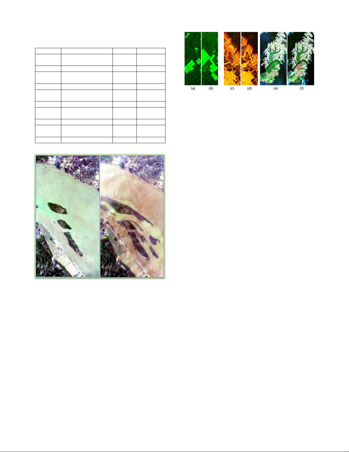
IEEE TRANSA CTIONS ON GEOSCIENCE AND REMO TE SENSING 1 GETNET : A General End-to-end T wo-dimensional CNN Frame work for Hyperspectral Image Change Detection Qi W ang, Senior Member , IEEE , Zhenghang Y uan, Qian Du, F ellow , IEEE , and Xuelong Li, F ellow , IEEE Abstract —Change detection (CD) is an important application of remote sensing, which pr ovides timely change inf ormation about large-scale Earth surface. With the emergence of hyper - spectral imagery , CD technology has been greatly pr omoted, as hyperspectral data with high spectral resolution are capable of detecting finer changes than using the traditional multispectral imagery . Nev ertheless, the high dimension of hyperspectral data makes it difficult to implement traditional CD algorithms. Be- sides, endmember abundance inf ormation at subpixel level is often not fully utilized. In order to better handle high dimension problem and explor e abundance information, this paper presents a General End-to-end T wo-dimensional CNN (GETNET) frame- work for hyperspectral image change detection (HSI-CD). The main contributions of this work are threefold: 1) Mixed-affinity matrix that integrates subpixel representation is introduced to mine mor e cr oss-channel gradient features and fuse multi-source information; 2) 2-D CNN is designed to learn the discriminativ e features effectively from multi-source data at a higher level and enhance the generalization ability of the proposed CD algorithm; 3) A new HSI-CD data set is designed for objective comparison of different methods. Experimental results on real hyperspectral data sets demonstrate the proposed method outperforms most of the state-of-the-arts. Index T erms —change detection (CD), hyperspectral image (HSI), mixed-affinity matrix, deep learning, 2-D CNN, spectral unmixing I . I N T R O D U C T I O N T HE comprehensi ve cognition of the global change is a critical task for providing timely and accurate infor- mation in the Earth’ s ev olution. Change detection (CD), as an important application of identifying differences of mul- titemporal remote sensing images, finds great use in land cov er mapping [1], natural disaster monitoring [2], resource exploration [3] and so forth. The complete CD process is mainly divided into three steps: (1) Image preprocessing, where multitemporal images are spatially and radiometrically processed with geometric correction, radiometric correction and noise reduction; (2) Change difference image generation, where change difference images are obtained to contrast changed and unchanged regions of multitemporal images; and This work was supported by the National K ey R&D Program of China under Grant 2017YFB1002202, National Natural Science Foundation of China under Grant 61773316, Fundamental Research Funds for the Central Univ ersities under Grant 3102017AX010, and the Open Research Fund of K ey Laboratory of Spectral Imaging T echnology , Chinese Academy of Sciences. 2019 IEEE. Personal use of this material is permitted. Permission from IEEE must be obtained for all other uses, in any current or future media, including reprinting/republishing this material for advertising or promotional purposes, creating ne w collecti ve works, for resale or redistribution to servers or lists, or reuse of any copyrighted component of this work in other works. (3) Evaluation, where a certain measure is used to assess the performance. Hyperspectral image (HSI) with high spectral resolution can provide richer spectral information than other remote sensing images, such as synthetic aperture radar (SAR) images [4] and multispectral images (MSIs) [5]. Thus, HSIs ha ve the potential to identify finer changes [6], with the detailed composition of different objects being reflected. Though HSI- CD methods have been dev eloped, it does not mean that the hyperspectral image change detection (HSI-CD) problem can be readily solved, for CD is a complicated process and can be affected by many factors. The main challenges for HSI-CD are summarized as follows. 1) Mixed pixel problem . In actual HSI-CD, mixed pixels commonly exist. A mixed pixel is a mixture of more than one distinct substance [7]. If one mixed pixel is roughly categorized into a certain kind of substance, it will not be expressed accurately . In general, mixed pixels may limit the improv ement of hyperspectral task if not being carefully handled. 2) High dimensionality . The high dimension of hyperspec- tral data makes it dif ficult to handle in some CD algorithms. In spite of the fact that feature extraction or band selection [8] is utilized to reduce the dimensionality , the detailed information may be lost to some extent. 3) Limited data sets . The data sets for HSI-CD are relativ ely limited, for constructing a ground-truth map that reflects real change information of ground objects requires considerable time and effort. Both field work and manual labeling are time consuming and expensiv e. Aiming at the aforementioned three challenges, our moti- vations are described in detail from two aspects. First, an in- depth analysis of internal pixel is necessary , but many related research are case studies on limited problems about HSI-CD. Spectral unmixing is a process to decompose a mixed pixel into a collection of endmembers and the corresponding abun- dance maps. An abundance map [7] indicates the proportion of a corresponding endmember present in the pixel, contain- ing much detailed subpixel composition. By considering the useful information, unmixing in HSI-CD not only enhances the performance [9], but also provides easily interpretable information for the nature of changes [10]. Though spectral unmixing has been widely studied, research on HSI-CD by unmixing is still in an early stage. Existing studies in the literature are case studies on certain problems and mainly focus on linear or nonlinear unmixing without combining them IEEE TRANSA CTIONS ON GEOSCIENCE AND REMO TE SENSING 2 in HSI-CD. Second, deep learning can better handle the problem of high dimension and exploit effecti ve features, but the features are not fully mined in many HSI-CD methods. By learning which part or what kind of combination of multi-source data is critical, deep learning of fers flexible approaches to deal with HSI. Generally , a change difference image can be obtained from the two preprocessed images with the trained deep neural network. Howe ver , many HSI-CD methods based on deep learning do not fully exploit the feature contained between the spectra of corresponding pixels in multitemporal images. These methods mainly analyze the changes of pixels by 1-D spectral vector . The features between the spectra of corresponding pixels contain richer information, which is often neglected. Based on the aforementioned two motiv ations, this paper dev elops a new general framework, namely GETNET for HSI- CD task. The main contributions are summarized as follows. (1) A simple yet ef fecti ve mixed-af finity matrix is proposed to better mine the changed patterns between two corre- sponding spectral vectors on a spatial pixel. Different from previous methods, mixed-affinity matrix con verts two 1-D pixel vectors to a 2-D matrix for CD task, which provides more abundant cross-channel gradient information. Moreover , mixed-af finity matrix can effec- tiv ely deal with multi-source data simultaneously and make it possible to learn representativ e features between the spectra in the GETNET . (2) A novel end-to-end framework named GETNET based on 2-D CNN is dev eloped to improve the generalization ability of HSI-CD algorithm. T o the best of our knowl- edge, GETNET is the first one to fuse HSI and abundance maps together to handle changes caused by different complicated factors. The proposed approach outperforms (or is competiti ve to) other methods across all the four data sets without parameter adjustment. Moreover , this approach offers more potential than other methods on some special data sets given that unmixing information is properly used. (3) A new HSI-CD data set named “riv er” in Fig. 5 is designed for objecti ve comparison of different methods, and the corresponding ground-truth map is shown in Fig. 10 (g). The changed information on this data set is relativ ely complicated and experimental results sho w that this data set we create is reliable and rob ust for quantitativ e assessment of CD task. The remainder of this paper is organized as follows. Section II revie ws the related work. Section III describes the detail of the proposed method. Section IV ev aluates the performances of different CD approaches. Finally , we conclude this paper in Section V. I I . R E L A T E D W O R K The most common and simple methods of CD are image differencing and image ratioing, mainly designed for single- band images. These two methods are easy to implement but their applicable scope is limited. When handling multi-band remote sensing images, classical CD methods fall primarily into four categories. 1) Image arithmetical oper ation . The most common ap- proach is change vector analysis (CV A) [11], which generates magnitude and direction of change by spectral vector subtrac- tion. Besides, there are many comparati ve analyses based on CV A, such as ICV A, MCV A and CV APS [12]. T ypically , based on the polar CV A, C 2 V A [13] describes the CD problem in a magnitude-direction 2-D representation produced by a loss compression procedure. In addition, Chen et al . [14] apply tensor algebra to CD and propose 4-D Higher Order Singular V alue Decomposition (4D-HOSVD) to capture comprehensive changed features. 2) Image transformation . Methods based on image trans- formation conv ert multispectral images into a specific feature space to emphasize changed pixels and suppress unchanged ones. As a linear transformation technique, Principal Compo- nent Analysis (PCA) [15] decorrelates images [16]. Ho we ver , PCA heavily relies on the statistical property of images and is especially vulnerable to unbalanced data [17]. Based on canonical correlation analysis, multiv ariate alteration detection (MAD) [18] is an unsupervised method to analyze multi- temporal images CD. Nevertheless, MAD is not applicable to affine transformation. Then, iterati vely re weighted multiv ariate alteration detection (IR-MAD) [19] extends MAD by applying different weights to observ ations. Howe ver , IR-MAD still cannot utilize the notable relationship between multitemporal bands. The subspace-based change detection (SCD) method [20] takes the observed pixel of one HSI as target, and estab- lishes the background subspace by utilizing the corresponding pixel in the other image. 3) Ima ge classification . These methods are supervised schemes and have prior knowledge for the training of a classifier . Among them, post-classification comparison (PCC) [13] takes the CD as an image pair classification task, where the two classified images are compared pixel by pixel. The pixels fall into different categories are considered as changed regions. This is also the case of classification of differential features [21] and compound classification [22]. 4) Other advanced methods . Research on deep learning has found significant use in CD of multi-band images. For example, Zhang et al . [15] de velop a deep belief network (DBN) based feature extraction method, which concatenates a pair of multitemporal vectors to output the deep representation used for CD. By reshaping pixels to vectors, Zhao et al . [23] present a restricted Boltzmann machine (RBM) based deep learning methods to learn representation for image analysis. In addition, more new approaches have been put forward to solve the problems of HSI-CD in the recent studies. Liu et al . [24] describe a hierarchical CD approach, aiming at distinguishing all the possible change types by considering discriminable spectral behaviors. Based on statistical analyses of spectral profiles, Han et al . [25] adopt an unsupervised CD algorithm for denoising without dimensionality reduction. The aforementioned four categories can be applied to HSIs, but the accuracy may be improved if mixed pixels are considered to handle pix el level change. In order to address mixed pixels in HSIs, unmixing is necessary . HSI-CD IEEE TRANSA CTIONS ON GEOSCIENCE AND REMO TE SENSING 3 0 0 0 A C C A E B D D 0 0 0 A C C A E B D D 0 0 0 A C C A E B D D 0 0 0 A C C A E B D D Mu l t i - t e m p or a l i nput L i n e a r U n m i x i n g N on - l i ne a r U n m i xi ng L i ne a r U nm i xi n g N on - l i ne a r U n m i x i ng C on c a t C on c a t C N N C N N FC C h a n g e d e t e ct i on r e s u l t E n d m e m b e r s e x t r a ct i o n Fig. 1. Overview of the GETNET CD method for multitemporal HSIs. by unmixing has obvious advantages of providing subpixel lev el information. Howe ver , unmixing in HSI-CD is very challenging and has not been extensi vely studied so far . The work in [26] obtains change difference image by calculat- ing changes between the corresponding abundance maps of multitemporal images. In addition to spectral information, superpixels are utilized to integrate spatial information in the unmixing process [27]. These two approaches detect changes in the abundance of multitemporal images for each endmember simply by dif ference operation, limited to certain problems. Liu et al . [28] analyzes abundance maps of changed and unchanged endmembers and their contribution to each pixel. Besides, sparse unmixing is firstly explored for HSI-CD by Ert ¨ urk et al . [10] with spectral libraries. Many studies about unmixing in change analysis are limited to case studies and need to be further explored. I I I . M E T H O D O L O G Y The overvie w of the proposed CD method for multitemporal HSIs is sho wn in Fig. 1. First, spectral unmixing algorithms are used to deal with two preprocessed HSIs. Then the abundance maps obtained by linear and nonlinear unmixing interact with the HSIs and form mix ed-affinity matrices. Next mix ed-affinity matrices are processed by the GETNET . In the end, the final CD result is the output of the deep neural network. In this section, we introduce our method from three aspects: hybrid-unmixing for subpixel lev el mining, mixed-af finity matrix generation for information fusion and GETNET with “separation and combination”. A. Hybrid-unmixing for Subpixel Level Mining In order to obtain subpixel level information and improv e generalization ability , spectral unmixing is utilized in the pro- posed method. A complete spectral unmixing process contains endmember extraction and abundance estimation. In previous studies, various endmember extraction algorithms(EEAs) are dev eloped and any EEA is applicable to the proposed method. In this work, automatic tar get generation process (A TGP) [29] is adopted to find potential target endmembers. After end- members are obtained, the next step is to achie ve abundance estimation, namely , abundance maps for each pixel. Aiming at achieving abundance estimation, mixture models can be di vided into two categories: linear and nonlinear . Either has advantages and is applicable to certain cases [30], [31]. Nev ertheless, fe w works pay attention to combining them in HSI-CD. In order to utilize both advantages, our study focuses on hybrid-unmixing, namely , not only linear but also nonlinear mixture model. The linear mixture model assumes that each pixel is a linear combination of endmembers and the reflectance r r r of one pixel can be expressed as r = m X i =1 w l i x i + ε = X w l + ε, (1) s.t. m X i =1 w l i = 1 , (2) 0 ≤ w l i ≤ 1 , i = 1 , 2 , 3 , ..., m, (3) where r r r represents a b × 1 vector; b is the number of HSI bands; m is the number of endmembers; X X X is a b × m matrix of endmembers; x i x i x i is the i th column of X X X ; w l w l w l is an m × 1 vector of linear abundance fraction; w l i denotes the linear proportion of the i th endmember; ε is a b × 1 vector of noise caused by the sensor and modelling errors. Eqs. (2) and (3) are two constraints of abundances non-negati ve constraint (ANC) and abundance sum-to-one constraint (ASC), respecti vely . T o estimate the parameters, the fully constrained least squares (FCLS) [32] method is adopted. The linear abundance map w l w l w l is the ke y information used in the proposed method. IEEE TRANSA CTIONS ON GEOSCIENCE AND REMO TE SENSING 4 Fig. 2. The mixed data cube of HSI and unmixing ab undance maps. The nonlinear mixture model can be formulated as r = m X i =1 w n i x i + m X i =1 m X j =1 a ij x i  x j + ε, (4) s.t. ∀ i ≥ j : a ij = 0 , (5) ∀ i < j : a ij = w n i w n j , (6) m X i =1 w n i = 1 , w n i ≥ 0 , (7) where  is the point-wise multiplication operator; a ij repre- sents the bilinear parameter to model the nonlinearity of HSIs; w n i denotes the nonlinear proportion of the i th endmember; Other parameters hav e the same meaning in Eq. (1). In this work, the bilinear-Fan model (BFM) [31] is employed to obtain the parameters and the nonlinear abundance map w n w n w n is achieved. It is worth noting that both inputs in one data set share the same endmembers. Specifically , all the endmembers used in FCLS and BFM algorithms are the same and generated by the A TGP algorithm. By applying simple and effecti ve methods, subpixel level information is explored fully to the next step. As linear and nonlinear mixture models are appropriate for different cases, combining both methods in a unified framework can improve the generalization ability . The size of HSI is h × w × b . For con venience, we stack all the w l w l w l (the number of w l w l w l is h × w ) into a 3-D abundance data cube with the size of h × w × m . w n w n w n is processed on the same way of w l w l w l . Then, the next step is to integrate the two types of abundance maps together with the hyperspectral data. In other words, three kinds of data are stacked neatly in sequence in the direction of HSI spectral domain, as shown in Fig. 2. The final multi-source data cube, with the size of w × h × ( b + 2 m ) , contains almost all the HSI information for the subsequent analysis. B. Mixed-af finity Matrix Generation for Information Fusion Different from the pre vious deep learning methods, this work proposes a novel mixed-affinity matrix for 2-D CNN algorithm. Assume there are b bands to represent one pixel in HSI. Moreov er , there are m different endmembers and each endmember has a complete linear and nonlinear abundance maps (the size of complete abundance map is h × w ). As described in Section. III-A, both pixel and subpixel level information of the integrated multi-source data cube is ob- tained. Hence, the similarity between different bands of the corresponding pixels is a kind of signature to describe this pixel, i.e., a certain band in one pixel interacts with other b bands in the corresponding pixel respecti vely . Meanwhile, the similarity between different abundance maps is also another signature to indicate subpixel representation. Then we define mixed-af finity matrix, which contains both pixel and subpixel lev el signatures to represent each pixel. The mixed-af finity matrix is constructed as K ij = 1 − ( r 1 ij − r 2 ij ) /r 2 ij , i, j = 1 , 2 , 3 , ..., N (8) where K ij is a 2-D mixed-affinity matrix of n × n and it represents the relationship between corresponding pixels of different wa velengths and abundance maps; N = h × w ; n = b + 2 m ; r 1 ij is a n × 1 vector of a pixel at time 1 in Fig. 2; r 2 is another n × 1 vector of the corresponding pixel at time 2 . Mixed-af finity matrix is a 2-D matrix of n × n and it represents the relationship between corresponding pixels of different wavelengths and abundance maps, i.e., mix ed-affinity . As illustrated in Fig. 3, mixed-af finity matrix is divided into fiv e different parts. In part A, a certain band at time 1 in one pixel subtracts from other b bands in the corresponding pixel at time 2 . Part A represents the pixel lev el difference information. In part B, linear abundance map of a certain endmember for one pixel at time 1 subtracts from the corresponding linear abundance map at time 2 . Similarly , in part E, nonlinear abundance map interacts with each other by subtraction. In part D, linear abundance map subtracts from the corresponding nonlinear abundance map. Part B, D and E rev eal subpixel lev el differ- ence information. As the affinity between hyperspectral data and abundance maps is meaningless, each K ij in part C is set to 0. In general, the image spectral affinity and abundance affinity are distributed in the left top and right bottom corner respectiv ely in Fig. 3. The greater value of K ij is, the more similar it is between the corresponding pixels. After the mixed-affinity matrices are calculated, they are input to the proposed 2-D CNN. The architecture takes the CD as a binary classification task and outputs the classification result shown in Fig. 4. Remarkably , the similarity and difference of the corresponding pixels can be seen from the value of mix ed-affinity matrix. Mixed-af finity matrix has important significance in three aspects as follows. 1) Mixed-af finity matrix is an efficient way for simultane- ous processing of multi-source information fusion, combining preprocessed hyperspectral data with linear and nonlinear abundance maps. In addition, pixel and subpixel lev el rep- resentation is achie ved naturally . 2) The differences between the two 1-D pixel vectors is mapped to a 2-D matrix, which provides more abundant cross-channel gradient information. By mining the differences among b channels and 2 m complete abundance maps, the utilization ratio of multi-source information is maximized. 3) The powerful learning ability of the 2-D CNN can work seamlessly with the mixed-af finity matrix. On the one hand, IEEE TRANSA CTIONS ON GEOSCIENCE AND REMO TE SENSING 5 b m b b b m 0 0 0 A C C A E B D D Fig. 3. Mixed-affinity matrix of one pixel. 0 1 I n p u t af f i n i t y m at r i x C N N FC O u t p u t 0 0 A C C A E B D D 0 0 A C C A E B D D 0 0 A C C A E B D D 0 0 A C C A E B D D Fig. 4. Architecture of the proposed CNN with mixed-affinity matrices for CD. deep learning is able to learn the significant features for CD task. On the other hand, it can integrate information with local context according to different parts in mixed-af finity matrix. C. GETNET with “Separation and Combination” CD can be seen as binary classification of changed and un- changed pixels. The proposed classification model on mixed- affinity matrix is different from a traditional CNN classi- fication task. In common image classification task, better performance is usually obtained by a deeper CNN model. This model commonly exploits residual layers or inception modules to learn powerful representations of images. Considering the specific CD task, we design a general end-to-end 2-D CNN architecture for the vector pair classification problem. The end-to-end architecture can help ensure high accuracy of the whole system by optimizing it at all layers and generate the change difference image without stage-wise optimization or error accumulation problem. Then, the designed network is introduced as follo ws. 1) “Separation and Combination” : The proposed algo- rithm inv olves con volution operators on the mixed-af finity matrices. The structure of mixed-af finity matrix is illustrated in Fig. 3, where the image spectral affinity and abundance affinity are distributed in the left top and right bottom corner respectiv ely . T raditional conv olution operation shares kernel weights on the whole input map. Howe ver , it is not suitable for the mixed-affinity matrix at the early con volution layer, since spectral feature has dif ferent nature compared with the abundance map. In this work, two dif ferent con volution kernels are operated on the mixed-af finity matrix. One is for the image spectral af finity in the left top, i.e., part A, and the other is for the ab undance af finity in the right bottom corner , i.e., part B, D and E. Because the v alue of part C is 0, any conv olution kernel is applicable here. Then we adopt the locally sharing weights con volution [33] for these parts. After locally sharing conv olution layers and max pooling layers on the mixed-af finity matrices, two kinds of higher lev el features of dif ferent parts, i.e., spectral feature and abundance feature, are learned automatically by the proposed network. The next step is to classify these features by the fully connected layers, which work as a classifier . Additionally , considering the truth that dif ferent data sets are sensitiv e to different types of features, the fully connected layers are employed to fuse these features to improv e the generalization ability . 2) T raining with Pre-detection : The overall architecture of the proposed network is shown in Fig. 4, and the detailed parameters are presented in T able I, where the LS stands for locally sharing weights con volution [33]. In this work, HSI- CD is vie wed as a binary classification task of changed and unchanged pixels. Mixed-af finity matrices are input into the 2-D CNN and the outputs of network are the class labels of pixels. A change difference image can be obtained from the two HSIs with the trained network. Howev er, the ground- truth map is used to ev aluate the different CD methods but not for training in HSI analysis. Thus, we need to generate pseudo data sets to train it. Any HSI-CD method can be used to generate labeled samples. This research adopts the con ventional method CV A with high confidence threshold to generate pseudo training sets with labels. Pixels which hav e high possibility of being classified correctly are selected as final labeled samples to train the network. The positiv e samples (changed samples) account for about 10% of the changed pixels. The number of negati ve samples (unchanged samples) is twice of the positiv e samples, namely that the ratio of positi ve to negati ve samples is 1 : 2. The number of training samples has a significant impact on the performance of classification. If the positiv e and negati ve training samples are unbalanced, the network may be biased to the class with more samples. T o avoid this, the ratio between the positi ve and negati ve samples is set to 1:1 at first. Ho wever , more training samples is desired to train a deep network without pre-trained models. According to the pre-detection method (CV A) output, the ratio between the changed and unchanged samples is usually far less than 1:1. Thus more unchanged samples are needed to train the network. Then the ratio of positiv e to negati ve samples is set to 1 : 2 in this model. I V . E X P E R I M E N T S In this section, extensiv e experiments are conducted using four real HSI data sets. Firstly , we introduce the existing and newly constructed data sets used in the experiments. Then ev aluation measures are described for HSI-CD methods. In the end, the experimental performances of the proposed method and other state-of-the-arts are analyzed in detail. A. Datasets Description The most important reason for the lack of HSI-CD data sets is that it is difficult to construct a ground-truth map. Ground-truth map is a change difference image reflecting the real change information of ground objects, composed of IEEE TRANSA CTIONS ON GEOSCIENCE AND REMO TE SENSING 6 T ABLE I A R C H I T E C T U R E D E TAI L S F O R G E T N E T . Layers T ype Channels Kernel Size LSCon v1 LSCon volution + BN Activ ation(tanh) 32 5 x 5 MaxPool1 MaxPooling - 2 x 2 LSCon v2 LSCon volution + BN Activ ation(tanh) 64 3 x 3 MaxPool2 MaxPooling - 2 x 2 LSCon v3 LSCon volution + BN Activ ation(tanh) 128 3 x 3 MaxPool3 MaxPooling - 2 x 2 LSCon v4 LSCon volution + BN Activ ation(tanh) 96 1 x 1 MaxPool4 MaxPooling - 2 x 2 FC1 Fully Connected + BN Activ ation(tanh) 512 - FC2 Fully Connected 2 - Fig. 5. The newly constructed data set of HSIs at two different time: (a) The riv er imagery on May 3, 2013, (b) The river imagery on December 31, 2013. changed and unchanged class. Each data set contains three images, two real HSIs which are taken at the same position from different times, and a ground-truth map. Generally , the structure of ground-truth map mainly depends on the on-the- spot in vestigation and some algorithms with high accurac y . For uncertain pixels, it is necessary to query their spectral values for further judgment. Constructing precise ground-truth map is vital for its quality directly affects accuracy assessment. In this work, all the HSI data sets used in the experiments are selected from Earth Observing-1 (EO-1) Hyperion images. The EO-1 Hyperion covers the 0.4-2.5 microns spectral range, with 242 spectral bands. Moreover , it provides a spectral resolution of 10 nm approximately , as well as a spatial resolution of 30 m. Though there are 242 spectral bands in Hyperion, the HSI quality can be harshly affected by the atmosphere. T ypically , some of spectral bands are noisy with low signal-to-noise ratio (SNR). Therefore, according to the ( a ) ( b ) ( c ) ( d ) ( e ) ( f ) Fig. 6. The existing experimental data sets in our paper: (a) The farmland imagery on May 3, 2006, (b) The farmland imagery on April 23, 2007, (c) The countryside imagery on No vember 3, 2007, (d) The countryside imagery on November 28, 2008, (e) The Poyang lake imagery on July 27, 2002, (f) The Poyang lake imagery on July 16, 2004. existing research and ENVI analysis, bands with high SNR are selected in the following analysis. The experiments are carried out on the data sets after noise elimination and the ground-truth maps of existing data sets come from [34]. 1) Existing Data Sets : There are some av ailable hyper- spectral data sets for HSI-CD methods. The first data set “farmland” is shown in Fig. 6 (a) and (b). It covers farmland near the city of Y ancheng, Jiangsu province, China, with a size of 450 × 140 pixels. The two HSIs were acquired on May 3, 2006, and April 23, 2007, respectively . There are 155 bands selected for CD after noise elimination. V isually , the main change on this data is the size of farmland. In this experiment, about 20.95% pixels of the whole image are selected as labeled samples, with 4400 positiv e samples and 8800 negati ve samples. There are more samples selected than other data sets because the proportion of changed pixels is higher . The second data set “countryside” is sho wn in Fig. 6 (c) and (d), which covers countryside near the city of Nantong, Jiangsu province, China, having a size of 633 × 201 pixels. The multitemporal HSIs were obtained on November 3, 2007 and Nov ember 28, 2008, respecti vely . 166 bands are selected for CD after noise elimination. V isually , the main change on this data is the size of rural areas. In this e xperiment, about 7.55% pixels are selected as labeled samples, with 3200 positiv e samples and 6400 negati ve samples. The third data set “Poyang lake” is sho wn in Fig. 6 (e) and (f). It cov ers the province of Jiangxi, China, with 394 × 200 pixels. The two HSIs were obtained on July 27, 2002 and July 16, 2004, respectively . 158 bands are a vailable for CD after noise elimination. V isually , the main change type on this data is the land change. In this experiment, about 2.17% pixels are selected, where 570 positi ve samples and 1140 negati ve samples are taken as labeled data. 2) Newly Constructed Data Set : The newly constructed data set “river” 1 is shown in Fig. 5. The two HSIs were acquired at May 3, 2013, and December 31, 2013, respecti vely in Jiangsu province, China. This data set has a size of 463 × 241 pixels, with 198 bands av ailable after noisy band remov al. The main change type on this data is disappearance of substance in riv er . In this experiment, about 3.37% pixels 1 http://crabwq.github .io IEEE TRANSA CTIONS ON GEOSCIENCE AND REMO TE SENSING 7 T ABLE II C O N F U S I O N M A T R I X Confusion Matrix Predicted 1 0 Actual 1 TP FN 0 FP TN are selected as labeled samples, with 1250 positiv e samples and 2500 negati ve samples. B. Evaluation Measures In order to ev aluate the performance of CD methods, we compare the change dif ference images with ground-truth maps, in which white pixels represent changed portions and black pixels mean unchanged parts. The accuracy of result can directly reflect the reliability and practicability of the CD methods. Generally , through pixel lev el ev aluation, this paper adopts three ev aluation criteria: ov erall accuracy(O A), Kappa coefficient and confusion matrix. In their calculation, there are four index es: 1) true positives (TP), i.e., the number of correctly-detected changed pixels. 2) true negati ves (TN), i.e., the number of correctly-detected unchanged pixels. 3) false positiv es (FP), i.e., the number of false-alarm pixels, and 4) the false negati ves (FN), i.e., the number of missed changed pixels. The overall accuracy (OA) is defined as O A = T P + T N T P + T N + F P + F N . (9) Kappa coefficient reflects the agreement between a final change difference image and the ground-truth map. Compared to O A, Kappa coef ficients can more objecti vely indicate the accuracy of the CD results. The higher value of Kappa coefficient, the better result of CD will be. Kappa coef ficient is calculated as K appa = O A − P 1 − P , (10) where P = ( T P + F P )( T P + F N ) ( T P + T N + F P + F N ) 2 + ( F N + T N )( F P + T N ) ( T P + T N + F P + F N ) 2 (11) As illustrated in T able II, a confusion matrix represents information about predicted and actual binary classifications (changed and unchanged classifications) conducted by CD algorithms, and it indicates how the instances are distributed in estimated and true classes. C. Experimental r esults In this work, the changes between HSIs are at pixel level variation with no subpixel lev el change in volved. Spectral unmixing is utilized to obtain subpixel level information, which can improve the performance of pixel level CD. In order to demonstrate the effecti veness and generality of the proposed method, we compare it with other state-of-the-art methods, including change vector analysis (CV A) [35], prin- cipal component analysis- change vector analysis (PCA-CV A) [36], iterativ ely reweighed multi v ariate alteration detection ( a ) ( b ) ( c ) ( d ) ( e ) ( f ) ( g ) Fig. 7. The change difference images of different methods on the data set of farmland, (a) the change difference image of CV A, (b) PCA-CV A, (c) IR-MAD, (d) SVM, (e) CNN, (f) GETNET , and (g) ground-truth map. (IRMAD) [19], support vector machines (SVM) [21], and patch-based con volutional neural network (CNN), which takes preprocessed HSIs as input. The principle for choosing these algorithms is due to their variety and popularity . Specifically , they employ different techniques to detect changes, such as image arithmetical operation, image transformation and deep learning. For the setup of experiments, the proposed GETNET is implemented by using Keras with T ensorflow as backend. The modified detail of the CNN network architecture is shown in T able I. The GETNET is trained from scratch and no pre- trained models are used in this work. The batch size used for training is set to 96. The optimizer is Adagrad with epsilon 10 − 8 and initial learning rate is set to 10 − 4 without decay . The training parameter setups are the same on all data sets, which are trained with 30000 steps. The OA and Kappa coefficients of six CD methods on different data sets are sho wn in T able III. T o ev aluate the proposed GETNET , we run 5 times per data set and get the mean value together with the standard deviation as the final CD results. The results in T able III show that GETNET is rob ust across different data sets with the same parameter setting. The histogram of the O A comparisons on four data sets in different methods is shown in Fig. 11. The confusion matrices compare the performance of CNN and GETNET method in Fig. 12. The comparisons of OA in GETNET and GETNET without unmixing are illustrated in Fig. 13. 1) Experiments on the F armland Data Set : As sho wn in Fig. 7, the main change is the size of farmland on this data set. T able III gives the details of different methods on four data sets. After overall consideration of O A and Kappa coefficient, it can be obviously found that GETNET is an effecti ve method for CD task. W ith respect to O A, con ventional CV A, PCA-CV A and IR-MAD perform better than CNN, but the performance of SVM is poor . Generally , SVM, CNN and GETNET use semi-supervised learning to train the classifier and network with the same training sets. Therefore, noise in pseudo training set can hav e negativ e effect on the accuracy of semi-supervised learning. SVM, as a binary classifier , di vides the image into changed and unchanged areas but cannot deal adequately with noise. Moreover , CNN based deep learning is also not effecti ve as expected, for it is more easily affected by noise in pseudo training set. As can be clearly seen, the best satisfactory performance is IEEE TRANSA CTIONS ON GEOSCIENCE AND REMO TE SENSING 8 T ABLE III T H E OV E R A L L AC C U R A C Y A N D K A P PA C O E FFI C I E N T S O F G E T N E T A N D OT H E R D I FF E R E N T S TA T E - O F - T H E - A R T C H A N G E D E T E C T I O N M E T H O D S O N F O U R DAT A S E T S Different methods Index The experiment datasets farmland countryside Poyang lake riv er CV A O A 0.9523 0.9825 0.9693 0.9529 Kappa 0.8855 0.9548 0.8092 0.7967 PCA-CV A O A 0.9668 0.9276 0.9548 0.9437 Kappa 0.9202 0.8216 0.7259 0.7326 IR-MAD O A 0.9604 0.8568 0.8248 0.8963 Kappa 0.9231 0.8423 0.7041 0.6632 SVM O A 0.8420 0.9536 0.9583 0.9046 Kappa 0.6417 0.8767 0.7266 0.6360 CNN O A 0.9347 0.9033 0.9522 0.9440 Kappa 0.8504 0.7547 0.8412 0.6867 GETNET(without unmixing) O A 0.9765 ± 0.00332 0.9758 ± 0.00649 0.9760 ± 0.00258 0.9497 ± 0.00119 Kappa 0.9367 ± 0.00417 0.9438 ± 0.00219 0.8903 ± 0.00395 0.7662 ± 0.00377 GETNET(Ours, with unmixing) O A 0.9783 ± 0.00599 0.9851 ± 0.00126 0.9856 ± 0.00365 0.9514 ± 0.00482 Kappa 0.9572 ± 0.00495 0.9651 ± 0.00173 0.9113 ± 0.00408 0.7539 ± 0.00349 ( a ) ( b ) ( c ) ( d ) ( e ) ( f ) ( g ) Fig. 8. The change difference images of different methods on the data set of countryside, (a) the change difference image of CV A, (b) PCA-CV A, (c) IR-MAD, (d) SVM, (e) CNN, (f) GETNET , and (g) ground-truth map. ( a ) ( b ) ( c ) ( d ) ( e ) ( f ) ( g ) Fig. 9. The change difference images of different methods on the data set of Poyang lake, (a) the change difference image of CV A, (b) PCA-CV A, (c) IR-MAD, (d) SVM, (e) CNN, (f) GETNET , and (g) ground-truth map. provided by the proposed GETNET , since it makes full use of hyperspectral data with abundance information and high anti-noise property . Even GETNET without unmixing works well and achieves the second-best performance. From another respect, the Kappa coefficient of GETNET is also high, which means the agreement between GETNET and the ground-truth map is almost perfect. 2) Experiments on the Countryside Data Set : The size of rural areas is the primary change and the changed infor- mation is quite complicated as shown in Fig. 8. In this data set, the best performance is GETNET . Specifically , IR-MAD yields lower OA, for it is not very sensitiv e to complicated changes. Because of dimension-reduction, PCA-CV A loses a ( a ) ( b ) ( c ) ( d ) ( e ) ( f ) ( g ) Fig. 10. The change difference images of different methods on the data set of riv er , (a) the change difference image of CV A, (b) PCA-CV A, (c) IR-MAD, (d) SVM, (e) CNN, (f) GETNET , and (g) ground-truth map. farmland .70 .75 .80 .85 .90 .95 1.00 CVA PCA-CVA IRMAD SVM CNN GETNET poyang lake countryside river OA Fig. 11. The OA comparisons on four data sets in different methods. part of information producing worse performance than CV A. Although the OA of CNN reaches more than 90%, GETNET is appropriate 8% higher . This is primarily because the inputs of them are dif ferent. The patch-based CNN only exploits the spatial context information of the preprocessed HSIs, while GETNET utilizes mixed-af finity matrix, which is an ef ficient way for simultaneous processing of hyperspectral data with abundance maps. It is worth noting that GETNET and CV A achiev e a high O A of ov er 98%. GETNET without unmixng yields lower O A than CV A, since pseudo training sets may be IEEE TRANSA CTIONS ON GEOSCIENCE AND REMO TE SENSING 9 C N N G E T N E T f a r m l a n d c o u n t r y s i d e P o y a n g l a k e r i v e r Fig. 12. The confusion matrices of the patch-based CNN and GETNET . not sufficient to effecti vely train a deep network. Remarkably , abundance information provides subpixel level presentation, which improves the performance of CD. Though this data set is more complicated, both O A and Kappa coefficient of GETNET are e ven improved than other data sets. 3) Experiments on the P oyang Lake Data Set : On this data set, there are some dispersed changes cov ering the lake. The performance of IR-MAD is not very satisfactory in terms of both O A and Kappa coefficient, for it cannot separate various changes well. CV A, PCA-CV A and SVM methods are relativ ely insensitiv e to changes in the width of the spacers. The Kappa coefficients of PCA-CV A, IR-MAD and SVM are also lo w . Though CNN and GETNET are both based on deep learning, their performances are different. As can be seen in Fig. 9, some of obvious changes are not recognized well by CNN. Ho wever , GETNET is able to identify dispersed changes and changes in the width of the spacers. Overall, the best performance is generated by GETNET on this data set and GETNET without unmixing comes second at OA. 4) Experiments on the River Data Set : The disappearance of substance in riv er is an obvious change, and beyond that there are some dispersed changes. Fig. 10 details the visual comparison of six different methods. In this dataset, the best result is CV A but not GETNET . It is thought that GETNET should always perform better than CV A because of the pseudo training sets generated by CV A. Howe ver , in a few data sets, these generated data sets may be insufficient to effecti vely train a deep network without parameter adjustment. The performances of CV A and GETNET are very close, both generating O A up to 95%. PCA-CV A and CNN have the similar accuracy about 94%. Besides, IR-MAD offers lower O A and Kappa coefficient, for it cannot identify irregular changes well. In addition, a remarkable problem is that the Kappa coefficient of each method is relativ ely lo wer than other data set. This is because the data set is more complicated and include div erse changes. It also demonstrates that the data set we create is reliable. 5) Ablation study of GETNET : In this work, a mixed- affinity matrix is constructed as the input of 2-D CNN for discriminativ e features extraction. As illustrated in Fig. 3, abundance maps are used to provide extra subpix el infor- mation to improve the performance of CD. T o validate the effecti veness of the unmixing information, we carry out the experiments of GETNET with and without abundance maps. The experimental results are shown in Fig. 13, which demon- strate that GETNET is almost always better than GETNET without unmixing information across all the four data sets, since subpixel lev el representation is of good use to CD. Moreov er , it can also be seen from the line chart that the performance of GETNET is stable and robust on different data sets and weight initials. Although both GETNET and CNN are based on deep learning, the performance of GETNET is better according to T able III and Fig. 12. On the one hand, GETNET with end-to-end manner to train the deep neural network, can av oid error accumulation of some deep learning methods with pipeline procedure. On the other hand, the fusion of multi- sourced data, including hyperspectral data and unmixing abun- dance information, makes GETNET mine the characteristics of spectral gradient producing higher robustness, accuracy and generalization. The proposed method outperforms the other CD methods in most of the cases and is robust for different HSIs. The data sets used in the experiments in volve multiple change types, which demonstrate the merits of GETNET . The merits are mainly due to the nov el mixed-affinity matrix with abundant information and unique design of GETNET . V . C O N C L U S I O N In this paper, a general framew ork named GETNET is proposed for HSI-CD task by 2-D CNN. First, a novel mixed- affinity matrix is designed. It not only is an ef ficient way for simultaneous processing of multi-source information fusion, but also provides more abundant cross-channel gradient infor- mation. Next, based on deep learning, GETNET is developed IEEE TRANSA CTIONS ON GEOSCIENCE AND REMO TE SENSING 10 c o u n t r y s i d e f ar m l an d P o y an g l ak e r i v er Fig. 13. The comparisons of O A in GETNET and GETNET without unmixing to learn a series of more significant features fully mined, with excellent capabilities of generalization and robustness. Moreov er , a new HSI-CD data set is designed for objective comparison of different methods. In the end, the proposed method is ev aluated on existing and newly constructed data sets and shows its effecti veness through extensi ve comparisons and analyses. R E F E R E N C E S [1] Lorenzo Bruzzone and Sebastiano B. Serpico, “ An iterati ve technique for the detection of land-cover transitions in multitemporal remote-sensing images, ” IEEE T rans. Geoscience and Remote Sensing , vol. 35, no. 4, pp. 858–867, 1997. [2] A. K oltunov and S. L. Ustin, “Early fire detection using non-linear multitemporal prediction of thermal imagery , ” Remote Sensing of En vir onment , vol. 110, no. 1, pp. 18–28, 2007. [3] T uomas Hame, Istvan Heiler, and Jesus San Miguel-A yanz, “ An unsupervised change detection and recognition system for forestry , ” International Journal of Remote Sensing , vol. 19, no. 6, pp. 1079–1099, 1998. [4] Thu Trang Lł, V an Anh Tran, Ha Thai Pham, and Truong Tran Xuan, “Change detection in multitemporal sar images using a strategy of multistage analysis, ” pp. 152–165, 2017. [5] S. Gandhimathi Alias Usha, S. V asuki, S. Gandhimathi Alias Usha, and S. V asuki, “Unsupervised change detection of multispectral imagery using multi level fuzzy based deep representation, ” Journal of Asian Scientific Resear ch , vol. 7, 2017. [6] Andrew P T ewkesbury , Alexis J Comber, Nicholas J T ate, Alistair Lamb, and Peter F Fisher , “ A critical synthesis of remotely sensed optical image change detection techniques, ” Remote Sensing of Envir onment , vol. 160, pp. 1–14, 2015. [7] Nirmal Keshav a and John F Mustard, “Spectral unmixing, ” IEEE signal pr ocessing magazine , vol. 19, no. 1, pp. 44–57, 2002. [8] Qi W ang, Fahong Zhang, and Xuelong Li, “Optimal clustering framew ork for hyperspectral band selection, ” IEEE T ransactions on Geoscience and Remote Sensing , pp. 1–13, 2018. [9] C-C Hsieh, P-F Hsieh, and C-W Lin, “Subpixel change detection based on abundance and slope features, ” in Geoscience and Remote Sensing Symposium, 2006. IGARSS 2006. IEEE International Confer ence on . IEEE, 2006, pp. 775–778. [10] Alp Ert ¨ urk, Marian Daniel Iordache, and Antonio Plaza, “Sparse unmixing-based change detection for multitemporal hyperspectral im- ages, ” IEEE Journal of Selected T opics in Applied Earth Observations And Remote Sensing , vol. 9, no. 2, pp. 708–719, 2015. [11] Osmar A Carvalho J ´ unior , Renato F Guimar ˜ aes, Alan R Gillespie, Nilton C Silva, and Roberto A T Gomes, “ A new approach to change vector analysis using distance and similarity measures, ” Remote Sensing , vol. 3, no. 11, pp. 2473–2493, 2011. [12] Francesca Bovolo and Lorenzo Bruzzone, “ A theoretical frame work for IEEE TRANSA CTIONS ON GEOSCIENCE AND REMO TE SENSING 11 unsupervised change detection based on change vector analysis in the polar domain, ” IEEE T ransactions on Geoscience And Remote Sensing , vol. 45, no. 1, pp. 218–236, 2007. [13] Francesca Bovolo, Silvia Marchesi, and Lorenzo Bruzzone, “ A frame- work for automatic and unsupervised detection of multiple changes in multitemporal images, ” IEEE T ransactions on Geoscience And Remote Sensing , vol. 50, no. 6, pp. 2196–2212, 2012. [14] Zhao Chen, Bin W ang, Y ubin Niu, W ei Xia, Jian Qiu Zhang, and Bo Hu, “Change detection for hyperspectral images based on tensor analysis, ” in Geoscience and Remote Sensing Symposium , 2015, pp. 1662–1665. [15] Hui Zhang, Maoguo Gong, Puzhao Zhang, Linzhi Su, and Jiao Shi, “Feature-lev el change detection using deep representation and feature change analysis for multispectral imagery , ” IEEE Geoscience And Remote Sensing Letters , vol. 13, no. 11, pp. 1666–1670, 2016. [16] T urgay Celik, “Unsupervised change detection in satellite images using principal component analysis and k -means clustering, ” IEEE Geoscience And Remote Sensing Letters , vol. 6, no. 4, pp. 772–776, 2009. [17] JS Deng, K W ang, YH Deng, and GJ Qi, “Pca-based land-use change detection and analysis using multitemporal and multisensor satellite data, ” International Journal of Remote Sensing , vol. 29, no. 16, pp. 4823–4838, 2008. [18] Allan A. Nielsen, Knut Conradsen, and James J. Simpson, “Multi variate alteration detection (mad) and maf postprocessing in multispectral, bitemporal image data: New approaches to change detection studies, ” Remote Sensing of Envir onment , vol. 64, no. 1, pp. 1–19, 1997. [19] A. A. Nielsen, “The regularized iteratively reweighted mad method for change detection in multi- and hyperspectral data., ” IEEE T ransactions on Image Pr ocessing A Publication of the IEEE Signal Pr ocessing Society , vol. 16, no. 2, pp. 463–78, 2007. [20] Chen W u, Bo Du, and Liangpei Zhang, “ A subspace-based change detection method for hyperspectral images, ” IEEE Journal of Selected T opics in Applied Earth Observations And Remote Sensing , vol. 6, no. 2, pp. 815–830, 2013. [21] Hassiba Nemmour and Y oucef Chibani, “Multiple support vector machines for land cover change detection: An application for mapping urban extensions, ” Isprs Journal of Photogrammetry and Remote Sensing , vol. 61, no. 2, pp. 125–133, 2006. [22] Lorenzo Bruzzone and Sebastiano B Serpico, “ An iterative technique for the detection of land-cover transitions in multitemporal remote-sensing images, ” IEEE T ransactions on Geoscience and Remote Sensing , vol. 35, no. 4, pp. 858–867, 1997. [23] Jiaojiao Zhao, Maoguo Gong, Jia Liu, and Licheng Jiao, “Deep learning to classify difference image for image change detection, ” in Neural Networks (IJCNN), 2014 International Joint Confer ence on . IEEE, 2014, pp. 411–417. [24] Sicong Liu, Lorenzo Bruzzone, Francesca Bovolo, and Peijun Du, “Hi- erarchical unsupervised change detection in multitemporal hyperspectral images, ” IEEE T ransactions on Geoscience And Remote Sensing , vol. 53, no. 1, pp. 244–260, 2015. [25] Y oukyung Han, Anjin Chang, Seokkeun Choi, Honglyun Park, and Jaew an Choi, “ An unsupervised algorithm for change detection in hyperspectral remote sensing data using synthetically fused images and deriv ative spectral profiles, ” Journal of Sensors,2017,(2017-8-10) , vol. 2017, pp. 1–14, 2017. [26] Alp Ert ¨ urk and Antonio Plaza, “Informati ve change detection by unmixing for hyperspectral images, ” IEEE Geosci. Remote Sensing Lett. , vol. 12, no. 6, pp. 1252–1256, 2015. [27] Alp Ert ¨ urk, Sarp Ert ¨ urk, and Antonio Plaza, “Unmixing with slic superpixels for hyperspectral change detection, ” in Geoscience and Remote Sensing Symposium , 2016, pp. 3370–3373. [28] Sicong Liu, Lorenzo Bruzzone, Francesca Bovolo, and Peijun Du, “Multitemporal spectral unmixing for change detection in hyperspectral images, ” in Geoscience and Remote Sensing Symposium , 2015, pp. 4165–4168. [29] Hsuan Ren and Chein I Chang, “ Automatic spectral target recognition in hyperspectral imagery , ” Aer ospace and Electr onic Systems IEEE T ransactions on , v ol. 39, no. 4, pp. 1232–1249, 2010. [30] Jie Chen, C. Richard, and P . Honeine, “Nonlinear unmixing of hy- perspectral data based on a linear-mixture/nonlinear -fluctuation model, ” IEEE T ransactions on Signal Pr ocessing , vol. 61, no. 2, pp. 480–492, 2013. [31] Jie Y u, Dongmei Chen, Y i Lin, and Su Y e, “Comparison of linear and nonlinear spectral unmixing approaches: a case study with multispectral tm imagery , ” International Journal of Remote Sensing , vol. 38, no. 3, pp. 773–795, 2017. [32] D. C. Heinz and Chein-I-Chang, “Fully constrained least squares linear spectral mixture analysis method for material quantification in hyperspectral imagery , ” IEEE T ransactions on Geoscience and Remote Sensing , vol. 39, no. 3, pp. 529–545, 2002. [33] Gary B Huang, Honglak Lee, and Erik Learned-Miller, “Learning hierarchical representations for face verification with con volutional deep belief networks, ” in Computer V ision and P attern Recognition (CVPR), 2012 IEEE Confer ence on . IEEE, 2012, pp. 2518–2525. [34] Y uan Y uan, Haobo Lv , and Xiaoqiang Lu, “Semi-supervised change detection method for multi-temporal hyperspectral images, ” Neur ocom- puting , vol. 148, pp. 363–375, 2015. [35] W . A Malila, “Change v ector analysis: an approach for detecting forest changes with landsat [remote sensing; idaho], ” 1980. [36] Munmun Baisantry , D. S. Negi, and O. P . Manocha, “Change vec- tor analysis using enhanced pca and inv erse triangular function-based thresholding, ” Defence Science Journal , vol. 62, no. 4, pp. 236–242, 2012. Qi W ang (M’15-SM’15) received the B.E. degree in automation and the Ph.D. degree in pattern recog- nition and intelligent systems from the Univ ersity of Science and T echnology of China, Hefei, China, in 2005 and 2010, respectiv ely . He is currently a Professor with the School of Computer Science, with the Unmanned System Research Institute, and with the Center for OPTical IMagery Analysis and Learn- ing, Northwestern Polytechnical University , Xi’an, China. His research interests include computer vi- sion and pattern recognition. Zhenghang Y uan received the B.E. degree in information security from the Northwestern Polytechnical Uni versity , Xi’an, China, in 2017. She is currently working toward the M.S. degree in computer science in the Center for OPT ical IMagery Analysis and Learning, Northwestern Polytechnical Univ ersity , Xi’an, China. Her research interests include hyperspectral image processing and computer vision. Qian Du (S’98-M’00-SM’05-F’17) received the Ph.D. degree in electrical engineering from the University of MarylandBaltimore County , Baltimore, MD, USA, in 2000. She is currently a Bobby Shackouls Professor with the Department of Electrical and Computer Engineering, Mississippi State Univ ersity , Starkville, MS, USA. Her research interests include hyperspectral remote sensing image analysis and applications, pattern classification, data compression, and neural networks. Xuelong Li (M’02-SM’07-F’12) is a Full Professor with the Center for Op- tical Imagery Analysis and Learning, Xi’an Institute of Optics and Precision Mechanics, Chinese Academy of Sciences, Xi’an 710119, China.