Deep Reinforcement Learning for Unmanned Aerial Vehicle-Assisted Vehicular Networks

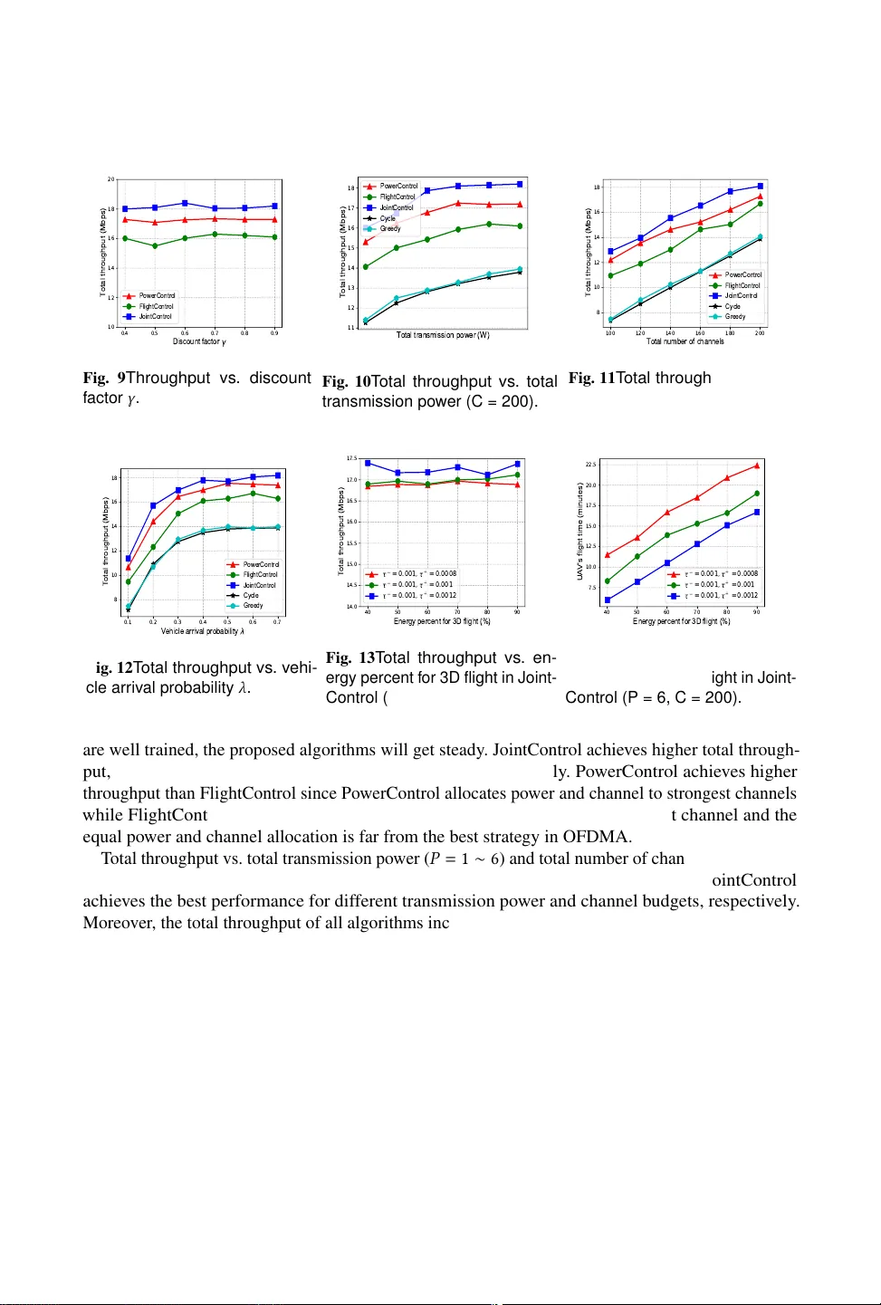
21 Deep Reinf or cement Learning f or Unmanned Aerial V ehic le-Assisted V ehicular Netw orks MING ZHU, Shenzhen Institutes of Advanced T echnology , Chinese Academy of Sciences, China XIA O-Y ANG LIU * , Department of Electrical Engineering, Columbia Univ ersity, USA ANW AR W ALID, Nokia Bell Labs, USA Unmanned aerial vehicles (U A Vs) are en visioned to complement the 5G communication infrastructure in future smart cities. Hot spots easily appear in road intersections, where ef fectiv e communication among vehicles is challenging. U A Vs may serve as relays with the adv antages of lo w price, easy deployment, line-of-sight links, and flexible mobility . In this paper , we study a U A V -assisted vehicular netw ork where the U A V jointly adjusts its transmission control (po wer and channel) and 3D flight to maximize the total throughput. First, we formulate a Marko v decision process (MDP) problem by modeling the mobility of the U A V/vehicles and the state transitions. Secondly , we solve the target problem using a deep reinforcement learning method, namely , the deep deterministic policy gradient (DDPG), and propose three solutions with different control objecti ves. Deep reinforcement learning methods obtain the optimal policy through the interactions with the en vironment without knowing the en vironment v ariables. Considering that en vironment variables in our problem are unkno wn and unmeasurable, we choose a deep reinforcement learning method to solv e it. Moreov er , considering the energy consumption of 3D flight, we e xtend the proposed solutions to maximize the total throughput per unit ener gy . T o encourage or discourage the U A V’ s mobility according to its prediction, the DDPG framew ork is modified, where the U A V adjusts its learning rate automatically . Thirdly , in a simplified model with small state space and action space, we verify the optimality of proposed algorithms. Comparing with tw o baseline schemes, we demonstrate the effecti v eness of proposed algorithms in a realistic model. CCS Concepts: • Theory of computation → Reinfor cement learning ; • A pplied computing → T ransporta- tion ; Multi-criterion optimization and decision-making . Additional K ey W ords and Phrases: Unmanned aerial vehicle, vehicular networks, smart cities, Marko v decision process, deep reinforcement learning, power control, channel control. A CM Reference Format: Ming Zhu, Xiao-Y ang Liu, and Anwar W alid. 2024. Deep Reinforcement Learning for Unmanned Aerial V ehicle-Assisted V ehicular Networks. A CM J . Auton. T ransport. Syst. 32, 14, Article 21 (February 2024), 28 pages. https://doi.org/10.1145/nnnnnnn.nnnnnnn INTRODUCTION Intelligent transportation system [ 11 ] [ 55 ] is a ke y component of smart cities, which employs real- time data communication for traf fic monitoring, path planning, entertainment and adv ertisement [ 26 ]. * Both authors contributed equally to this research. Authors’ addresses: Ming Zhu, zhumingpassional@gmail.com, Shenzhen Institutes of Advanced T echnology , Chinese Academy of Sciences, China; Xiao-Y ang Liu, xl2427@columbia.edu, Department of Electrical Engineering, Columbia Univ ersity, USA; Anwar W alid, anwar .walid@nokia- bell- labs.com, Nokia Bell Labs, USA. Permission to make digital or hard copies of all or part of this work for personal or classroom use is granted without fee provided that copies are not made or distributed for profit or commercial adv antage and that copies bear this notice and the full citation on the first page. Copyrights for components of this work owned by others than A CM must be honored. Abstracting with credit is permitted. T o copy otherwise, or republish, to post on servers or to redistrib ute to lists, requires prior specific permission and /or a fee. Request permissions from permissions@acm.org. © 2024 Association for Computing Machinery . 2833-0528/2024/2-AR T21 $15.00 https://doi.org/10.1145/nnnnnnn.nnnnnnn A CM J. Auton. Transport. Syst., V ol. 32, No. 14, Article 21. Publication date: February 2024. 21:2 Ming Zhu, Xiao-Y ang Liu, and Anwar W alid D ow nl i nk B a s e s t a t i on Fig. 1 The scenar io of a U A V -assisted vehicular network. High speed vehicular networks [ 14 ] emerge as a key component of intelligent transportation systems that provide cooperati v e communications to improv e data transmission performance. W ith the increasing number of vehicles, the current communication infrastructure may not satisfy data transmission requirements, especially when hot spots (e.g., road intersections) appear during rush hours. Unmanned aerial vehicles (U A Vs) or drones [ 37 ] can complement the 4G/5G communication infrastructure, including vehicle-to-vehicle (V2V) communications, and vehicle-to-infrastructure (V2I) communications. Qualcomm has recei v ed a certification of authorization allo wing for UA V testing belo w 400 feet [ 3 ]; Huawei will cooperate with China Mobile to b uild the first cellular test network for regional logistics UA Vs [ 2 ]. Existing road side units (RSUs) and 5G stations can not adjust their 3D positions to obtain the best communication links since their positions are fix ed. The energy consumption of UA Vs can be very lo w compared with 5G stations and RSUs. The required energy in one day for 5G base station is 72 kWh (a macrocell) or 19.2 kWh (a small cell) [ 20 ], which is much larger than U A Vs [ 1 ] and RSUs [ 5 ]. A U A V -assisted vehicular network has se v eral advantages. First, the path loss will be much lo wer since the U A V can move nearer to vehicles compared with stationary base stations. Secondly , the U A V is flexible in adjusting the 3D position with the mobility of vehicles so that the communication performance [ 9 ] is improv ed. Thirdly , the quality of U A V -to-vehicle links can be optimized by adjusting the U A V’ s 3D positions, and is generally better than that of terrestrial links [ 21 ], since there will be more radio frequencies and the LoS can be flexibly obtained. Existing road side units (RSUs) can not adjust their 3D positions to obtain the best communication links since they are fixed on road sides. Maximizing the total throughput of UA V -to-vehicle links has sev eral challenges. First, the commu- nication channels v ary with the U A V’ s 3D positions since various obstructions may lead to NLoS links, and the U A V’ s 3D position (especially height) affects the LoS/NLoS probability . Secondly , the joint adjustment of the U A V’ s 3D flight and transmission control (e.g., power control) cannot be solved directly using con ventional optimization methods with unknown and unmeasurable en viron- ment variables. Thirdly , the channel conditions are hard to acquire, e.g., the path loss from the U A V to vehicles is closely related to the height/density of b uildings and street width. Existing works focuses on the U A V’ s two-dimensional (2D) path planning [ 19 ], or the communi- cation control [ 43 ], or the joint control of them [ 48 ] [ 51 ] [ 53 ]. Most of them relies on the accurate parameters, howe ver , in 5G networks, it is not easy to measure the parameters accurately . In 5G A CM J. Auton. Transport. Syst., V ol. 32, No. 14, Article 21. Publication date: February 2024. Deep Reinforcement Learning f or Unmanned Aerial V ehicle-Assisted V ehicular Networks 21:3 networks, the strength of signals reduces significantly if the communication links are NLoS. The U A V can adjust its 3D position to obtain line-of-sight (NLoS) links. Generally , the UA V’ s height largely af fect the LoS/NLoS probability , therefore af fects the communication performance. Some current deep reinforcement learning (RL) based methods [ 52 ] [ 33 ] [ 38 ] can solve the U A V control or the communication control problem with unknown parameters. Howe v er , most of them do not consider the 3D movement of the UA Vs, the mov ement patterns of vehicles under the control of the traffic lights, or the joint control of the above two types of actions. Besides, existing works assume the terminals are stationary , so that the mov ement patterns of terminals (e.g., v ehicles) are not considered. In this paper , we propose deep reinforcement learning based algorithms to maximize the total throughput of U A V -to-vehicle communications, which jointly adjusts the UA V’ s 3D flight and transmission control by learning through interacting with the en vironment. The U A V’ s 3D flight changes the 3D position so that better communication links can be obtained. The transmission control includes the power control and channel control aiming to impro ve the total throughput. The main contributions of this paper can be summarized as follows: 1) W e formulate the problem as a Markov decision process (MDP) problem to maximize the total throughput with the constraints of total transmission po wer and total channel. Extracting the mobility patterns of UA V and vehicles is a challenge. The mobility patterns of vehicles in models should sho w that they are affected by the traffic light state. The mobility patterns of the UA V should consider the encoding/decoding of the horizontal flight and vertical flight. 2) W e apply a deep reinforcement learning method, the deep deterministic policy gradient (DDPG), to solve the problem. DDPG is suitable to solve MDP problems with continuous states and actions. W e propose three solutions with different control objecti ves to jointly adjust the U A V’ s 3D flight and transmission control. Then we extend the proposed solutions to maximize the total throughput per energy unit. T o encourage or discourage the U A V’ s mobility , we modify the rew ard function and the DDPG framework. 3) W e verify the optimality of proposed solutions using a simplified model with small state space and action space. Finally , we provide extensi v e simulation results to demonstrate the effecti veness of the proposed solutions compared with two baseline schemes. The remainder of the paper is organized as follows. Section discusses related works. Section presents system models and problem formulation. Solutions are proposed in Section . Section presents the performance ev aluation. Section concludes this paper . 2 RELA TED WORKS The dynamic control for the U A V -assisted vehicular networks includes flight control and transmission control. Flight control mainly includes the planning of flight path, time, and direction. Y ang et al. [ 50 ] proposed a joint genetic algorithm and ant colony optimization method to obtain the best UA V flight paths to collect sensory data in wireless sensor networks. T o further minimize the U A Vs’ travel duration under certain constraints (e.g., energy limitations, f airness, and collision), Garraffa et al. [ 19 ] proposed a two-dimensional (2D) path planning method based on a column generation approach. Liu et al. [ 28 ] proposed a deep reinforcement learning approach to control a group of U A Vs by optimizing the flying directions and distances to achiev e the best communication coverage in the long run with limited energy consumption. The transmission control of UA Vs mainly concerns resource allocations, e.g., access selection, transmission power and bandwidth/channel allocation. W ang et al. [ 43 ] presented a power allocation strategy for U A Vs considering communications, caching, and energy transfer . In a U A V -assisted communication network, Y an et al. [ 49 ] studied a UA V access selection and base station band- width allocation problem, where the interaction among U A Vs and base stations was modeled as a Stackelber g game, and the uniqueness of a Nash equilibrium was obtained. A CM J. Auton. Transport. Syst., V ol. 32, No. 14, Article 21. Publication date: February 2024. 21:4 Ming Zhu, Xiao-Y ang Liu, and Anwar W alid Joint control of both U A Vs’ flight and transmission has also be considered. W u et al. [ 48 ] considered maximizing the minimum achie v able rates from a UA V to ground users by jointly optimizing the UA V’ s 2D trajectory and power allocation. Zeng et al. [ 51 ] proposed a conv ex optimization method to optimize the UA V’ s 2D trajectory to minimize its mission completion time while ensuring each ground terminal recov ers the file with high probability when the UA V disseminates a common file to them. Zhang et al. [ 53 ] considered the UA V mission completion time minimization by optimizing its 2D trajectory with a constraint on the connectivity quality from base stations to the UA V . Fan et al. [ 17 ] optimized the U A V’ s 3D flight and transmission control together; howe ver , the 3D position optimization was con verted to a 2D position optimization by the LoS link requirement. Most existing research works neglected adjusting U A Vs’ height to obtain better quality of links by av oiding v arious obstructions or NLoS links. This will reduce the service quality especially in cities especially with multiple viaducts, high buildings and trees. Approximate dynamic programming (ADP) and stochastic dual dynamic programming (SDDP) can solve MDP problems with large space. Most ADP based approaches focus on path planning of U A Vs or vehicles, e.g., how to av oid collision [ 40 ] and coordinate a team of heterogeneous autonomous vehicles [ 18 ] [ 56 ]. SDDP [ 16 ] methods search the state space which may occur with large probability , so that the computing efficienc y is improv ed. Both ADP and SDDP methods need all variables. Ho wever , measuring these variables in 5G networks requires a lot of labor and cost. Deep reinforcement learning (DRL) based methods have been used in 5G vehicular networks [ 57 ] to provide high quality-of-service (QoS) services. Challita et al. [ 10 ] proposed a deep reinforcement learning based method for a cellular U A V network by optimizing the 2D path and cell association to achiev e a tradeof f between maximizing ener gy efficienc y and minimizing both wireless latency and the interference on the path. A similar scheme is applied to provide intelligent traf fic light control in [ 29 ]. [ 12 ] studies the temporal effects of dynamic blockage in vehicular networks and proposes a DRL method (DDPG) to overcome dynamic blockage. [ 52 ] proposes a DRL method for a joint relay selection and power allocation problem in multihop 5G mmW ave de vice to device transmissions. [ 33 ] constructs an intelligent offloading framew ork for 5G-enabled vehicular networks by jointly utilizing licensed cellular spectrum and unlicensed channels. The deep double Q-learning network (DDQN) method is used to solve a subproblem, distributed cellular spectrum allocation. [ 35 ] studies joint allocation of the spectrum, computing, and storing resources in a multi-access edge computing based vehicular network. DDPG is used to solv e this problem to satisfy the QoS requirements. [ 13 ] studies the age of information a ware radio resource management for expected long-term performance optimization in a Manhattan grid vehicle-to-vehicle network. It decomposes the original MDP into a series of MDPs, and then uses long short-term memory and DRL to solv e it. [ 38 ] introduces U A Vs cell-free network for pro viding cov erage to vehicles entering a highw ay that is not cov ered. It uses DRL (actor-critic method) to control U A Vs to achieve ef ficient communication co verage. Ho we v er , these methods do not consider the 3D movement of the agent (RSUs, or U A Vs), the movement patterns of vehicle under the control of the traf fic lights, or joint control of transmission power and channels. In addition, most existing works assumed that the ground terminals are stationary; whereas in reality , some ground terminals move with certain patterns, e.g., vehicles mov e under the control of traf fic lights. This work studies a U A V -assisted vehicular network where the UA V’ s 3D flight and transmission control can be jointly adjusted, considering the mobility of vehicles in a road intersection. A CM J. Auton. Transport. Syst., V ol. 32, No. 14, Article 21. Publication date: February 2024. Deep Reinforcement Learning f or Unmanned Aerial V ehicle-Assisted V ehicular Networks 21:5 4 1 2 3 0 L i g h t 2 L i g h t 1 F l ow 1 F l ow 2 F l ow 2 F l ow 1 Fig. 2 A one-wa y-two-flow road intersection. T able 1 V ar iables in comm unication model ℎ 𝑖 𝑡 , 𝐻 𝑖 𝑡 channel power g ain and channel state from the U A V to a vehicle in block 𝑖 in time slot 𝑡 . 𝜓 𝑖 𝑡 Signal to interference and noise ratio (SINR) from the U A V to a vehicle in block 𝑖 in time slot 𝑡 . 𝑑 𝑖 𝑡 , 𝐷 𝑖 𝑡 horizontal distance and Euclidean distance between the U A V and a vehicle in block 𝑖 . 𝑃 , 𝐶 , 𝑏 total transmission power , total number of channels, and band- width of each channel. 𝜌 𝑖 𝑡 , 𝑐 𝑖 𝑡 transmission power and number of channels allocated for the vehicle in block 𝑖 in time slot 𝑡 . 3 SYSTEM MODELS AND PROBLEM FORMULA TION In this section, we first describe the traffic model and communication model, and then formulate the target problem as a Marko v decision process. The v ariables in the communication model are listed in T able 1 for easy reference. 3.1 Road Intersection Model and T raffic Model W e start with a one-way-two-flo w road intersection, as shown in Fig. 2 , while a much more compli- cated scenario in Fig. 6 will be described in Section . Fi v e blocks are numbered as 0, 1, 2, 3, and 4, where block 0 is the intersection. W e assume that each block contains at most one vehicle, indicated by binary variables 𝒏 = ( 𝑛 0 , . . ., 𝑛 4 ) ∈ { 0 , 1 } . There are two traf fic flows in Fig. 2 , • “Flo w 1": 1 → 0 → 3 ; • “Flo w 2": 2 → 0 → 4 . The traffic light 𝐿 has four configurations: • 𝐿 = 0 : red light for flow 1 and green light for flo w 2; • 𝐿 = 1 : red light for flow 1 and yello w light for flow 2; • 𝐿 = 2 : green light for flow 1 and red light for flo w 2; • 𝐿 = 3 : yellow light for flo w 1 and red light for flow 2. A CM J. Auton. Transport. Syst., V ol. 32, No. 14, Article 21. Publication date: February 2024. 21:6 Ming Zhu, Xiao-Y ang Liu, and Anwar W alid L = 0 L = 0 T i me slo t s : L = 0 L = 2 L = 2 L = 2 ... ... T ra f f i c li g ht st a te tra nsi tions 0 1 N - 1 N + 1 N + 2 2 N .. . .. . .. . .. . N L = 1 L = 3 2 N + 1 Flow 2 : Flow 1 : 0 1 N - 1 N N + 1 N + 2 2 N 2 N + 1 Fig. 3 T raffic light states along time. T ime is partitioned into slots with equal duration. The duration of a green or red light occupies 𝑁 time slots, and the duration of a yellow light occupies a time slot, which are shown in Fig. 3 . W e assume that each vehicle mo ves one block in a time slot if the traf fic light is green. 3.2 Communication Model W e focus on the downlink communications (UA V -to-vehicle), since they are directly controlled by the U A V . There are two channel states of each UA V -to-vehicle link, line-of-sight (LoS) and non-line-of-sight (NLoS). Let 𝑥 and 𝑧 denote the block (horizontal position) and height of the U A V respectiv ely , where 𝑥 ∈ { 0 , 1 , 2 , 3 , 4 } corresponds to these five blocks in Fig. 2 , and 𝑧 is discretized to multiple values. W e assume that the UA V stays above the fi ve blocks since the U A V trends to get nearer to vehicles. Ne xt, we describe the communication model, including the channel po wer gain, the signal to interference and noise ratio (SINR), and the total throughput. First, the channel po wer gain between the U A V and a vehicle in block 𝑖 in time slot 𝑡 is ℎ 𝑖 𝑡 with a channel state 𝐻 𝑖 𝑡 ∈ { NLoS , LoS } . ℎ 𝑖 is formulated as [ 9 ] [ 8 ] ℎ 𝑖 𝑡 = ( ( 𝐷 𝑖 𝑡 ) − 𝛽 1 , if 𝐻 𝑖 𝑡 = LoS , 𝛽 2 ( 𝐷 𝑖 𝑡 ) − 𝛽 1 , if 𝐻 𝑖 𝑡 = NLoS , (1) where 𝐷 𝑖 𝑡 is the Euclidean distance between the U A V and the vehicle in block 𝑖 in time slot 𝑡 , 𝛽 1 is the path loss exponent, and 𝛽 2 is an additional attenuation factor caused by NLoS connections. The probabilities of LoS and NLoS links between the U A V and a vehicle in block 𝑖 in time slot 𝑡 are [ 32 ] 𝑝 ( 𝐻 𝑖 𝑡 = LoS ) = 1 1 + 𝛼 1 exp ( − 𝛼 2 ( 180 𝜋 arctan 𝑧 𝑑 𝑖 𝑡 − 𝛼 1 ) ) , (2) 𝑝 ( 𝐻 𝑖 𝑡 = NLoS ) = 1 − 𝑝 ( 𝐻 𝑖 𝑡 = LoS ) , 𝑖 ∈ { 0 , 1 , 2 , 3 , 4 } , (3) where 𝛼 1 and 𝛼 2 are system parameters depending on the en vironment (height/density of buildings, and street width, etc.). W e assume that 𝛼 1 , 𝛼 2 , 𝛽 1 , and 𝛽 2 hav e fixed values among all blocks in an intersection. 𝑑 𝑖 𝑡 is the horizontal distance in time slot 𝑡 . The angle 180 𝜋 arctan 𝑧 𝑑 𝑖 𝑡 is measured in “degrees" with the range 0 ◦ ∼ 90 ◦ . Both 𝑑 𝑖 𝑡 and 𝑧 𝑡 are discrete variables, therefore, 𝐷 𝑖 𝑡 =  ( 𝑑 𝑖 𝑡 ) 2 + 𝑧 2 𝑡 is also a discrete variable. Secondly , the SINR 𝜓 𝑖 𝑡 in time slot 𝑡 from the U A V to a vehicle in block 𝑖 is characterized as [ 34 ] 𝜓 𝑖 𝑡 = 𝜌 𝑖 𝑡 ℎ 𝑖 𝑡 𝑏𝑐 𝑖 𝑡 𝜎 2 , 𝑖 ∈ { 0 , 1 , 2 , 3 , 4 } , (4) where 𝑏 is the equal bandwidth of each channel, 𝜌 𝑖 𝑡 and 𝑐 𝑖 𝑡 are the allocated transmission po wer and number of channels for the vehicle in block 𝑖 in time slot 𝑡 , respectiv ely , and 𝜎 2 is the additiv e white Gaussian noise (A WGN) power spectrum density , and ℎ 𝑖 is formulated by ( 1 ). W e assume that the A CM J. Auton. Transport. Syst., V ol. 32, No. 14, Article 21. Publication date: February 2024. Deep Reinforcement Learning f or Unmanned Aerial V ehicle-Assisted V ehicular Networks 21:7 U A V employs orthogonal frequency di vision multiple access (OFDMA) [ 22 ]; therefore, there is no interference among these channels. Thirdly , the total throughput (rew ard) of U A V -to-vehicle links is formulated as [ 36 ]  𝑖 ∈ { 0 , 1 , 2 , 3 , 4 } 𝑏𝑐 𝑖 𝑡 log ( 1 + 𝜓 𝑖 𝑡 ) =  𝑖 ∈ { 0 , 1 , 2 , 3 , 4 } 𝑏𝑐 𝑖 𝑡 log ( 1 + 𝜌 𝑖 𝑡 ℎ 𝑖 𝑡 𝑏𝑐 𝑖 𝑡 𝜎 2 ) . (5) 3.3 MDP Formulation The U A V aims to maximize the total throughput with the constraints of total transmission power and total channels:  𝑖 ∈ { 0 , 1 , 2 , 3 , 4 } 𝜌 𝑖 𝑡 ≤ 𝑃 ,  𝑖 ∈ { 0 , 1 , 2 , 3 , 4 } 𝑐 𝑖 𝑡 ≤ 𝐶 , 0 ≤ 𝜌 𝑖 𝑡 ≤ 𝜌 max , 0 ≤ 𝑐 𝑖 𝑡 ≤ 𝑐 max , 𝑖 ∈ { 0 , 1 , 2 , 3 , 4 } , where 𝑃 is the total transmission power , 𝐶 is the total number of channels, 𝜌 max is the maximum power allocated to a v ehicle, 𝑐 max is the maximum number of channels allocated to a vehicle, 𝜌 𝑖 𝑡 is a discrete variable, and 𝑐 𝑖 𝑡 is a nonnegati v e integer v ariable. In MDP formulation, discrete transmission power is used for modeling and to help readers better understand the Marko v property . Such a discrete formulation does not prev ent a continuous solution. In fact, in the proposed algorithms, the transmission power is treated as continuous v ariable. The U A V -assisted communication is modeled as a Markov decision process (MDP). The Marko v property is that the future is independent of the past gi ven the present. Let’ s discuss all state transition processes. 1) The next states of traf fic lights depend on their current states, which is interpreted by Fig. 3 . 2) The next 3D position of the U A V depends on its current 3D position and 3D flight action. 3) The next number of vehicles in each block depends on the v ehicles’ current positions, mov ement directions and the current states of traffic lights. 4) The channel states depend on the current 3D position of the U A V and the current positions of vehicles, which is reflected by ( 2 ) and ( 3 ) . There are two types of stochastic processes. On one hand, from ( 2 ) and ( 3 ), we kno w that the channel state of U A V -to-vehicle links follo ws a stochastic process. On the other hand, the arri val of v ehicles follo ws a stochastic process under the states of the traffic lights. Under the MDP framew ork, the state space S , action space A , re ward 𝑟 , policy 𝜋 , and state transition probability 𝑝 ( 𝑠 𝑡 + 1 | 𝑠 𝑡 , 𝑎 𝑡 ) of our problem can be defined. The MDP formulation can be extended to other network links with terminals moving with dif ferent speeds, e.g., the vehicle-to-RSU networks, the U A V networks, and the 5G station networks. • State S = ( 𝐿, 𝑥 , 𝑧 , 𝒏 , 𝑯 ) , where 𝐿 is the traffic light state, ( 𝑥 , 𝑧 ) is the U A V’ s 3D position with 𝑥 ∈ { 0 , 1 , 2 , 3 , 4 } being the block and 𝑧 being the height, and 𝑯 = ( 𝐻 0 , . . ., 𝐻 4 ) is the channel state from the U A V to each block 𝑖 ∈ { 0 , 1 , 2 , 3 , 4 } with 𝐻 𝑖 ∈ { NLoS , LoS } . Let 𝑧 ∈ [ 𝑧 min , 𝑧 max ] , where 𝑧 min and 𝑧 max are the U A V’ s minimum and maximum height, respecti vely . The block 𝑥 is the location projected from U A V’ s 3D position to the road. The channel state instead of the channel power gain is considered in the state space since the cost of testing the channel state is much lower than measuring the channel po wer gain. The recei ved signal strength indicator (RSSI) is a type of radio interface. Based on RSSI, ho w to obtain the channel state is a classification problem. The channel state can be provided by machine learning [ 24 ]: ensemble learning methods (e.g., random forests, and gradient boosting), support vector machine, and deep neural networks. A CM J. Auton. Transport. Syst., V ol. 32, No. 14, Article 21. Publication date: February 2024. 21:8 Ming Zhu, Xiao-Y ang Liu, and Anwar W alid S 3 S 2 S 4 S 1 0 0 0 0 S 0 6 6 1 3 Fig. 4 The position state transition diagram when the U A V’ s height is fixed. • Action A = ( 𝒇 , 𝝆 , 𝒄 ) denotes the action set. 𝑓 𝑥 denotes the horizontal flight, and 𝑓 𝑧 denotes the vertical flight, both of which constitute the UA V’ s 3D flight 𝒇 = ( 𝑓 𝑥 , 𝑓 𝑧 ) . W ith respect to horizontal flight, we assume that the UA V can hov er or flight to its adjacent block in a time slot, thus 𝑓 𝑥 ∈ { 0 , 1 , . . ., 7 } in Fig. 4 . W ith respect to vertical flight, we assume 𝑓 𝑧 ∈ { − 𝜈 , 0 , 𝜈 } , (6) which means that the U A V can fly downw ard 𝜈 meters, horizontally , and up 𝜈 meters in a time slot. The U A V’ s height changes as 𝑧 𝑡 + 1 = 𝑓 𝑧 𝑡 + 𝑧 𝑡 . (7) 𝝆 = ( 𝜌 0 𝑡 , . . ., 𝜌 4 𝑡 ) and 𝒄 = ( 𝑐 0 𝑡 , . . ., 𝑐 4 𝑡 ) are the transmission po wer and channel allocation actions for those fi ve blocks, respectively . In the throughput optimization problem, the po wer and channel control actions are two basic actions, since they directly affect the communication performance in ( 5 ) . The U A V’ s 3D flight is another action since it affects the LoS/NLoS probability of the links and the distance between the U A V and vehicles, therefore, it indirectly affects the communication performance. At the end of time slot 𝑡 , the U A V moves to a new 3D position according to action 𝒇 , and over time slot 𝑡 , the transmission power and number of channels are 𝝆 and 𝒄 , respectively . • Rew ard 𝑟 ( 𝑠 𝑡 , 𝑎 𝑡 ) = Í 𝑖 ∈ { 0 , 1 , 2 , 3 , 4 } 𝑏𝑛 𝑖 𝑡 𝑐 𝑖 𝑡 log ( 1 + 𝜌 𝑖 𝑡 ℎ 𝑖 𝑡 𝑏𝑐 𝑖 𝑡 𝜎 2 ) is the total throughput after a transition from state 𝑠 𝑡 to 𝑠 𝑡 + 1 taking action 𝑎 𝑡 . Note that the total throughput over the 𝑡 -th time slot is measured at the state 𝑠 𝑡 = ( 𝐿 𝑡 , 𝑥 𝑡 , 𝑧 𝑡 , 𝒏 𝑡 , 𝑯 𝑡 ) . • Policy 𝜋 is the strategy for the UA V , which maps states to a probability distribution o ver the actions 𝜋 : S → P ( A ) , where P ( ·) denotes probability distribution. In time slot 𝑡 , the U A V’ s state is 𝑠 𝑡 = ( 𝐿 𝑡 , 𝑥 𝑡 , 𝑧 𝑡 , 𝒏 𝑡 , 𝑯 𝑡 ) , and its policy 𝜋 𝑡 outputs the probability distribution over the action 𝑎 𝑡 . W e see that the policy indicates the action preference of the U A V . • State transition probability 𝑝 ( 𝑠 𝑡 + 1 | 𝑠 𝑡 , 𝑎 𝑡 ) formulated in ( 8 ) is the probability of the U A V entering the new state 𝑠 𝑡 + 1 , after taking the action 𝑎 𝑡 at the current state 𝑠 𝑡 . At the current state 𝑠 𝑡 = A CM J. Auton. Transport. Syst., V ol. 32, No. 14, Article 21. Publication date: February 2024. Deep Reinforcement Learning f or Unmanned Aerial V ehicle-Assisted V ehicular Networks 21:9 ( 𝐿 𝑡 , 𝑥 𝑡 , 𝑧 𝑡 , 𝒏 𝑡 , 𝑯 𝑡 ) , after taking the 3D flight and transmission control 𝑎 𝑡 = ( 𝒇 , 𝝆 , 𝒄 ) , the U A V mov es to the new 3D position ( 𝑥 𝑡 + 1 , 𝑧 𝑡 + 1 ) , and the channel state changes to 𝑯 𝑡 + 1 , with the traffic light changes to 𝐿 𝑡 + 1 and the number of vehicles in each block changes to 𝒏 𝑡 + 1 . The state transitions of the traf fic light along time are sho wn in Fig. 3 . The transition of the channel state for U A V -to-vehicle links is a stochastic process, which is reflected by ( 2 ) and ( 3 ). Next, we discuss the MDP in three aspects: the state transition probability , the state transitions of the number of vehicles in each block, and the U A V’ s 3D position. Note that the transmission po wer control and channel control do not af fect the traf fic light, the channel state, the number of v ehicles, and the U A V’ s 3D position. First, we discuss the state transition probability 𝑝 ( 𝑠 𝑡 + 1 | 𝑠 𝑡 , 𝑎 𝑡 ) = 𝑝 ( ( 𝐿 𝑡 + 1 , 𝑥 𝑡 + 1 , 𝑧 𝑡 + 1 , 𝒏 𝑡 + 1 , 𝑯 𝑡 + 1 ) | ( 𝐿 𝑡 , 𝑥 𝑡 , 𝑧 𝑡 , 𝒏 𝑡 , 𝑯 𝑡 ) , ( 𝒇 𝑡 , 𝝆 𝑡 , 𝒄 𝑡 ) ) . The U A V’ s 3D fight only affects the U A V’ s 3D position state and the channel state, the traffic light state of the next time slot relies on the current traf fic light state, and the number of vehicles in each block of the ne xt time slot relies on the current number of vehicles and the traffic light state. Therefore, the state transition probability is 𝑝 ( 𝑠 𝑡 + 1 | 𝑠 𝑡 , 𝑎 𝑡 ) = 𝑝 ( 𝑥 𝑡 + 1 , 𝑧 𝑡 + 1 | 𝑥 𝑡 , 𝑧 𝑡 , 𝒇 𝑡 ) × 𝑝 ( 𝑯 𝑡 + 1 | 𝑥 𝑡 , 𝑧 𝑡 , 𝒇 𝑡 ) × 𝑝 ( 𝐿 𝑡 + 1 | 𝐿 𝑡 ) × 𝑝 ( 𝒏 𝑡 + 1 | 𝐿 𝑡 , 𝒏 𝑡 ) , (8) where 𝑝 ( 𝑥 𝑡 + 1 , 𝑧 𝑡 + 1 | 𝑥 𝑡 , 𝑧 𝑡 , 𝒇 𝑡 ) is easily obtained by the 3D position state transition based on the U A V’ s flight actions in Fig. 4 , 𝑝 ( 𝑯 𝑡 + 1 | 𝑥 𝑡 , 𝑧 𝑡 , 𝒇 𝑡 ) is easily obtained by ( 2 ) and ( 3 ), 𝑝 ( 𝐿 𝑡 + 1 | 𝐿 𝑡 ) is obtained by the traffic light state transition in Fig. 3 , and 𝑝 ( 𝒏 𝑡 + 1 | 𝐿 𝑡 , 𝒏 𝑡 ) is easily obtained by ( 9 ) ∼ ( 13 ). Secondly , we discuss the state transitions of the number of vehicles in each block. It is a stochastic process. The U A V’ s states and actions do not affect the number of vehicles of all blocks. Let 𝜆 1 and 𝜆 2 be the probabilities of the arriv als of new vehicles in flo w 1 and 2, respecti v ely . The state transitions for the number of vehicles in block 0, 3, and 4 are 𝑛 0 𝑡 + 1 =          𝑛 2 𝑡 , if 𝐿 𝑡 = 0 , 𝑛 1 𝑡 , if 𝐿 𝑡 = 2 , 0 , otherwise , (9) 𝑛 3 𝑡 + 1 = ( 𝑛 0 𝑡 , if 𝐿 𝑡 = 2 , 3 , 0 , otherwise , (10) 𝑛 4 𝑡 + 1 = ( 𝑛 0 𝑡 , if 𝐿 𝑡 = 0 , 1 , 0 , otherwise . (11) The transition probability is 1 in ( 9 ), ( 10 ) and ( 11 ) since the transitions are deterministic in block 0, 3, and 4. While the state transition probabilities for the number of vehicles in block 1 and 2 are nondeterministic, moreov er , both of them are af fected by their current number of vehicles and the traffic light. T aking block 1 when the traffic light state 𝐿 𝑡 = 2 as an example, the probability for the number of appeared vehicles is 𝑝 ( 𝑛 1 𝑡 + 1 = 1 | 𝐿 𝑡 = 2 ) = 𝜆 1 , (12) 𝑝 ( 𝑛 1 𝑡 + 1 = 0 | 𝐿 𝑡 = 2 ) = 1 − 𝜆 1 . (13) When ( 𝑛 1 𝑡 = 0 , 𝐿 𝑡 ≠ 2 ) and ( 𝑛 1 𝑡 = 1 , 𝐿 𝑡 ≠ 2 ) , the probability for the number of vehicles will be obtained in a similar way . A CM J. Auton. Transport. Syst., V ol. 32, No. 14, Article 21. Publication date: February 2024. 21:10 Ming Zhu, Xiao-Y ang Liu, and Anwar W alid Thirdly , we discuss the state transition of the U A V’ s 3D position. It includes horizontal position transitions and height transitions. The UA V’ s height transition is formulated in ( 7 ). If the U A V’ s height is fixed, the horizontal position transitions are sho wn in Fig. 4 , where { 𝑆 𝑖 } 𝑖 ∈ { 0 , 1 , 2 , 3 , 4 } denotes the block (i.e, horizontal position) of the U A V : 0 denotes staying in the current block; { 1 , 2 , 3 , 4 } denotes a flight from block 0 to the other blocks (1, 2, 3, and 4); 5 denotes an anticlockwise flight; 6 denotes a flight from block 1, 2, 3, or 4 to block 0; 7 denotes a clockwise flight. 4 PROPOSED SOLUTIONS In this section, we first describe the motiv ation, and then present an overvie w of Q-learning and the deep deterministic policy gradient (DDPG) algorithm, and then propose solutions with different control objectiv es, and finally present an extension of solutions that tak es into account the energy consumption of 3D flight. 4.1 Motivation The en vironment variables in this problem are unknown and unmeasurable. Deep reinforcement learning (RL) methods are suitable for the target problem for two reasons. First, DRL obtains the optimal policy through the interactions with the en vironment. Secondly , DRL does not need to know the environment variables. Neural networks are used to fit Q-value with the unknown and unmeasurable variables. F or e xample, 𝛼 1 and 𝛼 2 are affected by the height/density of b uildings, and the height and size of vehicles, etc. 𝛽 1 and 𝛽 2 are time dependent and are affected by the current en vironment such as weather [ 7 ]. Although UA Vs can detect the LoS/NloS links using equipped cameras, it is very challenging to detect them accurately for several reasons. First, the locations of recie vers on vehicles should be labeled for detection. Secondly , it is hard to detect recei vers accurately using computer vision technology since recei vers are much small than v ehicles. Thirdly , it requires automobile manufacturers to label the loactions of receivers, which may not be satisfied in sev eral years. Therefore, it requires a large amount of labor to test these en vironment variables accurately . It is hard to obtain the optimal strategies e ven all environment variables are known. Existing works [ 47 ] [ 54 ] obtain the near-optimal strategies in the 2D flight scenario when users are stationary , howe ver , they are not capable of solving our target problem since the U A V adjusts its 3D position and vehicles mo ve with their patterns under the control of traf fic lights. Q-learning cannot solve our problem because of se veral limitations. 1) Q-learning can only solve MDP problems with small state space and action space. Ho wever , the state space and action space of our problem are very lar ge. 2) Q-learning cannot solv e MDP problems with large state or action space since it may not conv er ge within reasonable time. W ith respect to continuous state/action space, the state/action should be discretized if using Q-learning. The U A V’ s transmission po wer allocation actions are continuous. The discrete transmission po wer in Section III is simply to illustrate the MDP formulation. 3) Q-learning will con v erge slo wly using too man y computational resources [ 41 ], and this is not practical in our problem. Therefore, we adopt the DDPG algorithm to solve our problem. 4.2 DDPG-based Algorithms The DDPG method [ 27 ] uses deep neural networks to approximate both action polic y 𝜋 and v alue function 𝑄 ( 𝑠 , 𝑎 ) . This method has two adv antages: 1) it uses neural networks as approximators, essentially compressing the state and action space to much smaller latent parameter space, and 2) the gradient descent method can be used to update the network weights, which greatly speeds up the con vergence and reduces the computational time. Therefore, the memory and computational resources are largely sav ed. In real systems, DDPG exploits the powerful skills introduced in AlphaGo A CM J. Auton. Transport. Syst., V ol. 32, No. 14, Article 21. Publication date: February 2024. Deep Reinforcement Learning f or Unmanned Aerial V ehicle-Assisted V ehicular Networks 21:11 Algorithm 1 : Environment simulation in one step (Fig. 4 as an e xample) 1: Select action 𝑎 according to line 3 in Alg. 3; 2: Generate random variables: probabilities of LoS and NLoS according to ( 2 ) and ( 3 ), respectiv ely; and the probability for the number of appeared v ehicles 𝜆 ; 3: Executing action 𝑎 , and determining the ne w state, including traffic light state according to Fig. 3 , the U A V’ s new 3D positions according to Fig. 4 and ( 7 ), and the number of vehicles in blocks according to ( 9 ) ∼ ( 13 ); 4: Calculate the rew ard 𝑟 using ( 5 ); 5: Update states, including traffic light state, U A V’ s 3D position and channel state, and the number of vehicles in blocks. zero [ 39 ] and Atari game playing [ 30 ], including experience replay buf fer , actor-critic approach, soft update, and exploration noise. 1) Experience replay buffer 𝑅 𝑏 stores transitions that will be used to update network parameters. At each time slot 𝑡 , a transition ( 𝑠 𝑡 , 𝑎 𝑡 , 𝑟 𝑡 , 𝑠 𝑡 + 1 ) is stored in 𝑅 𝑏 . After a certain number of time slots, each iteration samples a mini-batch of 𝑀 = | Ω | transitions { ( 𝑠 𝑗 , 𝑎 𝑗 , 𝑟 𝑗 , 𝑠 𝑗 ) } 𝑗 ∈ Ω to train neural networks, where Ω is a set of indices of sampled transitions from 𝑅 𝑏 . “Experience replay buf fer" has two advantages: 1) enabling the stochastic gradient decent method [ 15 ]; and 2) removing the correlations between consecutiv e transitions. 2) Actor-critic appr oach : the critic approximates the Q-value, and the actor approximates the action policy . The critic has two neural networks: the online Q-network 𝑄 with parameter 𝜃 𝑄 and the target Q-network 𝑄 ′ with parameter 𝜃 𝑄 ′ . The actor has tw o neural networks: the online policy network 𝜇 with parameter 𝜃 𝜇 and the target policy network 𝜇 ′ with parameter 𝜃 𝜇 ′ . The training of these four neural networks are discussed in the next subsection. 3) Soft update with a lo w learning rate 𝜏 ≪ 1 is introduced to impro ve the stability of learning. The soft updates of the target Q-netw ork 𝑄 ′ and the target polic y network 𝜇 ′ are as follows 𝜃 𝑄 ′ ← 𝜏 𝜃 𝑄 + ( 1 − 𝜏 ) 𝜃 𝑄 ′ = 𝜃 𝑄 ′ + 𝜏 ( 𝜃 𝑄 − 𝜃 𝑄 ′ ) , (14) 𝜃 𝜇 ′ ← 𝜏 𝜃 𝜇 + ( 1 − 𝜏 ) 𝜃 𝜇 ′ = 𝜃 𝜇 ′ + 𝜏 ( 𝜃 𝜇 − 𝜃 𝜇 ′ ) . (15) 4) Exploration noise is added to the actor’ s target polic y to output a new action 𝑎 𝑡 = 𝜇 ′ ( 𝑠 𝑡 | 𝜃 𝜇 ′ ) + N 𝑡 . (16) There is a tradeoff between exploration and exploitation, and the exploration is independent from the learning process. Adding exploration noise in ( 16 ) ensures that the U A V has a certain probability of exploring ne w actions besides the one predicted by the current policy 𝜇 ′ ( 𝑠 𝑡 | 𝜃 𝜇 ′ ) , and av oids that the U A V is trapped in a local optimum. 4.3 DDPG-based Solutions The UA V has two transmission controls, power and channel. W e use the power allocation as the main control objective for two reasons. 1) Once the po wer allocation is determined, the channel allocation will be easily obtained in OFDMA. According to Theorem 4 of [ 44 ], in OFDMA, if all links hav e the equal weights just as our reward function ( 5 ), the transmitter should send messages to the receiv er with the strongest channel in each time slot. In our problem, the strongest channel is not determined since the channel state (LoS or NLoS) is a random process. DDPG tends to allocate more power to the strongest channels with high probability , therefore, channel allocation will be easily A CM J. Auton. Transport. Syst., V ol. 32, No. 14, Article 21. Publication date: February 2024. 21:12 Ming Zhu, Xiao-Y ang Liu, and Anwar W alid Algorithm 2 : Channel allocation in time slot 𝑡 Input : the power allocation 𝝆 , the number of vehicles in all blocks 𝒏 , the maximum number of channels allocated to a vehicle 𝑐 max , the total number of channels 𝐶 . Output : the channel allocation 𝒄 𝑡 for all blocks. 1: Initialize the remaining total number of channels 𝐶 𝑟 ← 𝐶 . 2: Calculate the av erage allocated po wer for each vehicle in all blocks ¯ 𝝆 𝑡 by ( 17 ). 3: Sort ¯ 𝝆 𝑡 by the descending order , and obtain a sequence of block indices 𝑱 . 4: for block 𝑗 ∈ 𝑱 5: 𝑐 𝑗 𝑡 ← min ( 𝐶 𝑟 , 𝑛 𝑗 𝑡 𝑐 max ) . 7: 𝐶 𝑟 ← 𝐶 𝑟 − 𝑐 𝑗 𝑡 . 8: Return 𝒄 𝑡 . obtained based on power allocation actions. 2) Power allocation is continuous, and DDPG is suitable to handle these actions. Ho wev er , if we use DDPG for the channel allocation, the number of action variables will be v ery large and the con vergence will be very slo w , since the channel allocation is discrete and the number of channels is generally large (e.g., 200) especially in rush hours. W e choose power control or flight as control objecti ves since controlling power and flight is more ef ficient than controlling channel. Moreov er , the best channel allocation strategy can be obtained if the power is allocated in OFDMA. T o allocate channels among blocks, we introduce a variable denoting the a verage allocated po wer of a vehicle in block 𝑖 : ¯ 𝜌 𝑖 𝑡 = ( 𝜌 𝑖 𝑡 𝑛 𝑖 𝑡 , if 𝑛 𝑖 𝑡 ≠ 0 , 0 , otherwise . (17) The channel allocation algorithm is shown in Alg. 1, which is executed after obtaining the power allocation actions. As the above description, it achiev es the best channel allocation in OFDMA if the po wer allocation is kno wn [ 44 ]. Line 1 is the initialization. Lines 2 ∼ 3 calculate and sort ¯ 𝝆 𝑡 = { ¯ 𝜌 𝑖 𝑡 } 𝑖 ∈ { 0 , 1 , 2 , 3 , 4 } . Line 5 assigns the maximum number of channels to the current possibly strongest channel, and line 6 updates the remaining total number of channels. Based on the abov e analysis and Alg. 1, we propose three algorithms: • PowerControl: the U A V adjusts the transmission power allocation using the actor network at a fixed 3D position, and the channels are allocated to v ehicles by Alg. 1 in each time slot. • FlightControl: the U A V adjusts its 3D flight using the actor network, and the transmission power and channel allocation are equally allocated to each v ehicle in each time slot. • JointControl: the U A V adjusts its 3D flight and the transmission power allocation using the actor network, and the channels are allocated to vehicles by Alg. 1 in each time slot. The DDPG-based algorithms are giv en in Alg. 2. The algorithm has two parts: initializations, and the main process. Each episode finishes when the U A V ex ecutes a maximum number of steps, and the U A V’ s goal is to maximize the expected accumulated rew ard per episode. 𝑠 1 is the U A V’ s initial state. Generally , in each episode, 𝑠 1 is different so that the Q-v alue is trained well. First, we describe the initializations in lines 1 ∼ 3. In line 1, all states are initialized: the traffic light 𝐿 is initialized as 0, the number of vehicles 𝒏 in all blocks is 0, the U A V’ s block and height are randomized, and the channel state 𝐻 𝑖 for each block 𝑖 is set as LoS or NLoS with the same probability . Note that the action space DDPG controls in PowerControl, FlightControl, and JointControl is different. Line 2 initializes the parameters of the critic and actor . Line 3 allocates an experience replay buf fer 𝑅 𝑏 . A CM J. Auton. Transport. Syst., V ol. 32, No. 14, Article 21. Publication date: February 2024. Deep Reinforcement Learning f or Unmanned Aerial V ehicle-Assisted V ehicular Networks 21:13 Algorithm 3 : DDPG-based algorithms: PowerControl, FlightControl, and JointControl Input : the number of episodes 𝐾 , the number of time slots 𝑇 in an episode, the mini-batch size 𝑀 , the learning rate 𝜏 . 1: Initialize all states, including the traffic light state 𝐿 , the U A V’ s 3D position ( 𝑥 , 𝑧 ) , the number of vehicles 𝒏 and the channel state 𝑯 in all blocks. 2: Randomly initialize critic’ s online Q-network parameters 𝜃 𝑄 and actor’ s online policy network parameters 𝜃 𝜇 , and initialize the critic’ s target Q-network parameters 𝜃 𝑄 ′ ← 𝜃 𝑄 and actor’ s target policy network parameters 𝜃 𝜇 ′ ← 𝜃 𝜇 . 3: Allocate an experience replay b uf fer 𝑅 𝑏 . 4: for episode 𝑘 = 1 to 𝐾 5: Initialize a random process (a standard normal distribution) N for the U A V’ s action exploration. 6: Observe the initial state 𝑠 1 . 7: f or 𝑡 = 1 to T 8: Select the U A V’ s action ¯ 𝑎 𝑡 = 𝜇 ′ ( 𝑠 𝑡 | 𝜃 𝜇 ′ ) + N 𝑡 according to the policy of 𝜇 ′ and exploration noise N 𝑡 . 9: if PowerControl 10: Combine the channel allocation in Alg. 1 and ¯ 𝑎 𝑡 as the U A V’ s action 𝑎 𝑡 at a fixed 3D position. 11: if FlightControl 12: Combine the equal transmission power , equal channel allocation and ¯ 𝑎 𝑡 (3D flight) as the U A V’ s action 𝑎 𝑡 . 13: if JointControl 14: Combine the 3D flight action, the channel allocation in Alg. 1 and ¯ 𝑎 𝑡 as the U A V’ s action 𝑎 𝑡 . 15: Ex ecute the U A V’ s action 𝑎 𝑡 , and receiv e re ward 𝑟 𝑡 , and observe ne w state 𝑠 𝑡 + 1 from the en vironment. 16: Store transition ( 𝑠 𝑡 , 𝑎 𝑡 , 𝑟 𝑡 , 𝑠 𝑡 + 1 ) in the U A V’ s experience replay buf fer 𝑅 𝑏 . 17: Sample 𝑅 𝑏 to obtain a random mini-batch of 𝑀 transitions { ( 𝑠 𝑗 𝑡 , 𝑎 𝑗 𝑡 , 𝑟 𝑗 𝑡 , 𝑠 𝑗 𝑡 + 1 ) } 𝑗 ∈ Ω ⊆ 𝑅 𝑏 , where Ω is a set of indices of sampled transitions with | Ω | = 𝑀 . 18: The critic’ s target Q-network 𝑄 ′ calculates and outputs 𝑦 𝑗 𝑡 = 𝑟 𝑗 𝑡 + 𝛾 𝑄 ′ ( 𝑠 𝑗 𝑡 + 1 , 𝜇 ′ ( 𝑠 𝑗 𝑡 + 1 | 𝜃 𝜇 ′ ) | 𝜃 𝑄 ′ ) to the critic’ s online Q-network 𝑄 . 19: Update the critic’ s online Q-network 𝑄 to make its Q-value fit 𝑦 𝑗 𝑡 by minimizing the loss function: ∇ 𝜃 𝑄 Loss 𝑡 ( 𝜃 𝑄 ) = ∇ 𝜃 𝑄 [ 1 𝑀 Í 𝑀 𝑗 = 1 ( 𝑦 𝑗 𝑡 − 𝑄 ( 𝑠 𝑗 𝑡 , 𝑎 𝑗 𝑡 | 𝜃 𝑄 ) ) 2 ] . 20: Update the actor’ s online policy network 𝜇 based on the input { ∇ 𝑎 𝑄 ( 𝑠 , 𝑎 | 𝜃 𝑄 ) | 𝑠 = 𝑠 𝑗 𝑡 ,𝑎 = 𝜇 ( 𝑠 𝑗 𝑡 ) } 𝑗 ∈ Ω from 𝑄 using the policy gradient by the chain rule: 1 𝑀 Í 𝑗 ∈ Ω E 𝑠 𝑡 [ ∇ 𝑎 𝑄 ( 𝑠 , 𝑎 | 𝜃 𝑄 ) | 𝑠 = 𝑠 𝑡 ,𝑎 = 𝜇 ( 𝑠 𝑡 ) ∇ 𝜃 𝜇 𝜇 ( 𝑠 | 𝜃 𝜇 ) | 𝑠 = 𝑠 𝑡 ] . 21: Soft update the critic’ s target Q-network 𝑄 ′ and actor’ s target policy netw ork 𝜇 ′ to make the ev aluation of the UA V’ s actions and the U A V’ s policy more stable: 𝜃 𝑄 ′ ← 𝜏 𝜃 𝑄 + ( 1 − 𝜏 ) 𝜃 𝑄 ′ , 𝜃 𝜇 ′ ← 𝜏 𝜃 𝜇 + ( 1 − 𝜏 ) 𝜃 𝜇 ′ . Secondly , we present the main process. Line 5 initializes a random process for action exploration. Line 6 receiv es an initial state 𝑠 1 . Let ¯ 𝑎 𝑡 be the action DDPG controls, and 𝑎 𝑡 be the U A V’ s all action. Line 8 selects an action according to ¯ 𝑎 𝑡 and an exploration noise N 𝑡 . N 𝑡 is generated following a normal distribution. Lines 9 ∼ 10 combine the channel allocation actions in Alg. 1 and ¯ 𝑎 𝑡 as 𝑎 𝑡 at a fixed 3D position in Po werControl. Lines 11 ∼ 12 combine the equal transmission po wer , equal channel allocation actions and ¯ 𝑎 𝑡 (3D flight) as 𝑎 𝑡 in FlightControl. Lines 13 ∼ 14 combine the 3D flight action, the channel allocation actions in Alg. 1 and ¯ 𝑎 𝑡 as 𝑎 𝑡 in JointControl. Line 15 ex ecutes the U A V’ s action 𝑎 𝑡 , and then the U A V receives a re ward and all states are updated. Line 16 stores a transition into 𝑅 𝑏 . In line 17, a random mini-batch of transitions are sampled from 𝑅 𝑏 . Line 18 sets the value of 𝑦 𝑗 for the critic’ s online Q-network. Lines 19 ∼ 21 update all network parameters. A CM J. Auton. Transport. Syst., V ol. 32, No. 14, Article 21. Publication date: February 2024. 21:14 Ming Zhu, Xiao-Y ang Liu, and Anwar W alid How to obtain 3D flight and transmission po wer allocation in the action space in DDPG is an important issue. In fact, it is a mapping problem, i.e., how to encode and decode the two types of actions. The action space is separated to two parts, one for 3D flight (horizontal and the vertical flight) and the other for the transmission po wer allocation. The horizontal and the vertical flight actions are in a group, and the transmission power allocation actions are in the other group. Make sure that the locations of action v ariables match the ph ysical meaning as much as possible. T ake 8 horizontal flight actions in Fig. 2 as an example. W e use 8 v ariables to denote the probability of them, and we will choose the one with the largest probability as the horizontal flight action. The DDPG-based algorithms in Alg. 2 in essence are the approximated Q-learning method. The exploration noise in line 8 approximates the second case of ( 32 ) in Q-learning. Lines 18 ∼ 19 in Alg. 2 make  𝑟 𝑡 + 𝛾 max 𝑎 𝑡 + 1 𝑄 ( 𝑠 𝑡 + 1 , 𝑎 𝑡 + 1 ) − 𝑄 ( 𝑠 𝑡 , 𝑎 𝑡 )  con v erge. Line 20 of Alg. 2 approximates the first case of ( 32 ) in Q-learning, since both of them aim to obtain the policy of the maximum Q-value. In soft update of 𝑄 ′ in line 21 of Alg. 2, 𝜏 and 𝛼 are learning rates. Next, we discuss the training and test stages of proposed solutions. 1) In the training stage, we train the actor and the critic, and store the parameters of their neural networks. The training stage has two parts. First, 𝑄 and 𝜇 are trained through a random mini-batch of transitions sampled from the e xperience replay b uf fer 𝑅 𝑏 . Secondly , 𝑄 ′ and 𝜇 ′ are trained through soft update. The training process is as follows. A mini-batch of 𝑀 transitions { ( 𝑠 𝑗 𝑡 , 𝑎 𝑗 𝑡 , 𝑟 𝑗 𝑡 , 𝑠 𝑗 𝑡 + 1 ) } 𝑗 ∈ Ω are sampled from 𝑅 𝑏 , where Ω is a set of indices of sampled transitions from 𝑅 𝑏 with | Ω | = 𝑀 . Then two data flows are outputted from 𝑅 𝑏 : { 𝑟 𝑗 𝑡 , 𝑠 𝑗 𝑡 + 1 } 𝑗 ∈ Ω → 𝜇 ′ , and { 𝑠 𝑗 𝑡 , 𝑎 𝑗 𝑡 } 𝑗 ∈ Ω → 𝑄 . 𝜇 ′ outputs { 𝑟 𝑗 𝑡 , 𝑠 𝑗 𝑡 + 1 , 𝜇 ′ ( 𝑠 𝑗 𝑡 + 1 | 𝜃 𝜇 ′ ) } 𝑗 ∈ Ω to 𝑄 ′ to calculate { 𝑦 𝑗 𝑡 } 𝑗 ∈ Ω . Then 𝑄 calculates and outputs { ∇ 𝑎 𝑄 ( 𝑠 , 𝑎 | 𝜃 𝑄 ) | 𝑠 = 𝑠 𝑗 𝑡 ,𝑎 = 𝜇 ( 𝑠 𝑗 𝑡 ) } 𝑗 ∈ Ω to 𝜇 . 𝜇 updates its parameters by ( 20 ). Then two soft updates are executed for 𝑄 ′ and 𝜇 ′ in ( 14 ) and ( 15 ), respectiv ely . The data flow of the critic’ s target Q-network 𝑄 ′ and online Q-network 𝑄 are as follows. 𝑄 ′ takes { ( 𝑟 𝑗 𝑡 , 𝑠 𝑗 𝑡 + 1 , 𝜇 ′ ( 𝑠 𝑗 𝑡 + 1 | 𝜃 𝜇 ′ ) ) } 𝑗 ∈ Ω as the input and outputs { 𝑦 𝑗 𝑡 } 𝑗 ∈ Ω to 𝑄 . 𝑦 𝑗 𝑡 is calculated by 𝑦 𝑗 𝑡 = 𝑟 𝑗 𝑡 + 𝛾 𝑄 ′ ( 𝑠 𝑗 𝑡 + 1 , 𝜇 ′ ( 𝑠 𝑗 𝑡 + 1 | 𝜃 𝜇 ′ ) | 𝜃 𝑄 ′ ) . (18) 𝑄 takes n { 𝑠 𝑗 𝑡 , 𝑎 𝑗 𝑡 } 𝑗 ∈ Ω , o as the input and outputs { ∇ 𝑎 𝑄 ( 𝑠 , 𝑎 | 𝜃 𝑄 ) | 𝑠 = 𝑠 𝑗 𝑡 ,𝑎 = 𝜇 ( 𝑠 𝑗 𝑡 ) } 𝑗 ∈ Ω to 𝜇 for updating parameters in ( 20 ), where { 𝑠 𝑗 𝑡 } 𝑗 ∈ Ω are sampled from 𝑅 𝑏 , and 𝜇 ( 𝑠 𝑗 𝑡 ) = arg max 𝑎 𝑄 ( 𝑠 𝑗 𝑡 , 𝑎 ) . The data flo ws of the actor’ s online policy network 𝜇 and target polic y network 𝜇 ′ are as follo ws. After 𝑄 outputs { ∇ 𝑎 𝑄 ( 𝑠 , 𝑎 | 𝜃 𝑄 ) | 𝑠 = 𝑠 𝑗 𝑡 ,𝑎 = 𝜇 ( 𝑠 𝑗 𝑡 ) } 𝑗 ∈ Ω to 𝜇 , 𝜇 updates its parameters by ( 20 ). 𝜇 ′ takes { 𝑟 𝑗 𝑡 , 𝑠 𝑗 𝑡 + 1 } 𝑗 ∈ Ω as the input and outputs { 𝑟 𝑗 𝑡 , 𝑠 𝑗 𝑡 + 1 , 𝜇 ′ ( 𝑠 𝑗 𝑡 + 1 | 𝜃 𝜇 ′ ) } 𝑗 ∈ Ω to 𝑄 ′ for calculating { 𝑦 𝑗 𝑡 } 𝑗 ∈ Ω in ( 18 ), where { 𝑟 𝑗 𝑡 , 𝑠 𝑗 𝑡 + 1 } 𝑗 ∈ Ω are sampled from 𝑅 𝑏 . The updates of parameters of four neural networks ( 𝑄 , 𝑄 ′ , 𝜇 , and 𝜇 ′ ) are as follo ws. The online Q-network 𝑄 updates its parameters by minimizing the 𝐿 2 -norm loss function Loss 𝑡 ( 𝜃 𝑄 ) to make its Q-value fit 𝑦 𝑗 𝑡 : ∇ 𝜃 𝑄 Loss 𝑡 ( 𝜃 𝑄 ) = ∇ 𝜃 𝑄 [ 1 𝑀 𝑀  𝑗 = 1 ( 𝑦 𝑗 𝑡 − 𝑄 ( 𝑠 𝑗 𝑡 , 𝑎 𝑗 𝑡 | 𝜃 𝑄 ) ) 2 ] . (19) The target Q-network 𝑄 ′ updates its parameters 𝜃 𝑄 ′ by ( 14 ). The online policy network 𝜇 updates its parameters following the chain rule with respect to 𝜃 𝜇 : E 𝑠 𝑡 [ ∇ 𝜃 𝜇 𝑄 ( 𝑠 , 𝑎 | 𝜃 𝑄 ) | 𝑠 = 𝑠 𝑡 ,𝑎 = 𝜇 ( 𝑠 𝑡 | 𝜃 𝜇 ) ] = E 𝑠 𝑡 [ ∇ 𝑎 𝑄 ( 𝑠 , 𝑎 | 𝜃 𝑄 ) | 𝑠 = 𝑠 𝑡 ,𝑎 = 𝜇 ( 𝑠 𝑡 ) ∇ 𝜃 𝜇 𝜇 ( 𝑠 | 𝜃 𝜇 ) | 𝑠 = 𝑠 𝑡 ] . (20) A CM J. Auton. Transport. Syst., V ol. 32, No. 14, Article 21. Publication date: February 2024. Deep Reinforcement Learning f or Unmanned Aerial V ehicle-Assisted V ehicular Networks 21:15 The target polic y network 𝜇 ′ updates its parameters 𝜃 𝜇 ′ by ( 15 ). In each time slot 𝑡 , the current state 𝑠 𝑡 from the en vironment is deli v ered to 𝜇 ′ , and 𝜇 ′ calculates the U A V’ s target policy 𝜇 ′ ( 𝑠 𝑡 ) | 𝜃 𝜇 ′ . Finally , an exploration noise N is added to 𝜇 ′ ( 𝑠 𝑡 | 𝜃 𝜇 ′ ) to get the U A V’ s action in ( 16 ). 2) In the test stage, we restore the neural network of the actor’ s target polic y network 𝜇 ′ based on the stored parameters. This way , there is no need to store transitions to the experience replay b uf fer 𝑅 𝑏 . Gi ven the current state 𝑠 𝑡 , we use 𝜇 ′ to obtain the UA V’ s optimal action 𝜇 ′ ( 𝑠 𝑡 | 𝜃 𝜇 ′ ) . Note that there is no noise added to 𝜇 ′ ( 𝑠 𝑡 | 𝜃 𝜇 ′ ) , since all neural networks ha ve been trained and the U A V has got the optimal action through 𝜇 ′ . Finally , the U A V executes the action 𝜇 ′ ( 𝑠 𝑡 | 𝜃 𝜇 ′ ) . 4.4 Extension on Energy Consumption of 3D Flight The U A V’ s energy is used in two parts, communication and 3D flight. The above proposed solutions in Alg. 2 do not consider the energy consumption of 3D flight. In this subsection, we discuss how to incorporate the energy consumption of 3D flight into Alg. 2. T o encourage or discourage the UA V’ s 3D flight actions in different directions with different amount of energy consumption, we modify the rew ard function and the DDPG frame work. The U A V aims to maximize the total throughput per energy unit since the UA V’ s battery has limited capacity . For example, the U A V DJI Mavic Air [ 1 ] with full energy can only fly 21 minutes. Gi ven that the U A V’ s ener gy consumption of 3D flight is much lar ger than that of communication, we only use the former part as the total energy consumption. Thus, the re ward function ( 5 ) is modified as follows ¯ 𝑟 ( 𝑠 𝑡 , 𝑎 𝑡 ) = 1 𝑒 ( 𝑎 𝑡 )  𝑖 ∈ { 0 , 1 , 2 , 3 , 4 } 𝑏𝑛 𝑖 𝑡 𝑐 𝑖 𝑡 log ( 1 + 𝜌 𝑖 𝑡 ℎ 𝑖 𝑡 𝑏𝑐 𝑖 𝑡 𝜎 2 ) , (21) where 𝑒 ( 𝑎 𝑡 ) is the ener gy consumption of taking action 𝑎 𝑡 in time slot 𝑡 . 𝑒 ( 𝑎 𝑡 ) is calculated according to the U A V’ s energy consumption model for 3D flight. Alternati v ely , 𝑒 ( 𝑎 𝑡 ) can be measured easily by the follo wing way . The UA V has three vertical flight actions per time slot just as in ( 6 ). If the U A V keeps moving do wnward, horizontally , or upward until the energy for 3D flight is used up, the flight time is assumed to be 𝜙 𝑑 , 𝜙 ℎ , and 𝜙 𝑢 seconds, respecti vely . If the duration of a time slot is set to 𝜅 seconds, so the U A V can fly 𝜙 𝑑 𝜅 , 𝜙 ℎ 𝜅 , and 𝜙 𝑢 𝜅 time slots, respecti vely . Therefore, the formulation of 𝑒 ( 𝑎 𝑡 ) is gi ven by 𝑒 ( 𝑎 𝑡 ) =          𝜅 𝜙 𝑑 𝐸 full , if moving do wnward 𝜈 meters , 𝜅 𝜙 ℎ 𝐸 full , if moving horizontally , 𝜅 𝜙 𝑢 𝐸 full , if moving upward 𝜈 meters , (22) where 𝐸 full is the total energy if the U A V’ s battery is full. Let 𝛿 ( 𝑡 ) be a prediction error as follo ws 𝛿 ( 𝑡 ) = ¯ 𝑟 ( 𝑠 𝑡 , 𝑎 𝑡 ) − 𝑄 ( 𝑠 𝑡 , 𝑎 𝑡 ) , (23) where 𝛿 ( 𝑡 ) denotes the difference between the actual reward ¯ 𝑟 ( 𝑠 𝑡 , 𝑎 𝑡 ) and the expected return 𝑄 ( 𝑠 𝑡 , 𝑎 𝑡 ) . The prediction error is dif ferent from that in machine learning such as ensemble learning. In ensemble learning, the prediction error is the dif ference between predicted v alue and actual v alue. The learning rates here are adjusted follo wing the principle: when the prediction error is non-neg ativ e, a higher learning rate will be used, and a lower learning rate will be used otherwise. T o make the U A V learn from the prediction error 𝛿 ( 𝑡 ) , not the dif ference between the ne w Q-v alue and old Q-v alue in ( 31 ), A CM J. Auton. Transport. Syst., V ol. 32, No. 14, Article 21. Publication date: February 2024. 21:16 Ming Zhu, Xiao-Y ang Liu, and Anwar W alid the Q-value is updated by the follo wing rule 𝑄 ( 𝑠 𝑡 , 𝑎 𝑡 ) ← 𝑄 ( 𝑠 𝑡 , 𝑎 𝑡 ) + 𝛼 𝛿 ( 𝑡 ) ⇔ 𝑄 ( 𝑠 𝑡 , 𝑎 𝑡 ) ← 𝑄 ( 𝑠 𝑡 , 𝑎 𝑡 ) + 𝛼 ( ¯ 𝑟 ( 𝑠 𝑡 , 𝑎 𝑡 ) − 𝑄 ( 𝑠 𝑡 , 𝑎 𝑡 ) ) , (24) where 𝛼 is a learning rate similar to ( 31 ). W e introduce 𝛼 + and 𝛼 − to represent the learning rate when 𝛿 ( 𝑡 ) ≥ 0 and 𝛿 ( 𝑡 ) < 0 , respecti vely . Therefore, the U A V can choose to be acti v e or inacti ve by properly setting the v alues of 𝛼 + and 𝛼 − . The update of Q-value in Q-learning is modified as follo ws, inspired by [ 25 ] 𝑄 ( 𝑠 𝑡 , 𝑎 𝑡 ) ← 𝑄 ( 𝑠 𝑡 , 𝑎 𝑡 ) + ( 𝛼 + 𝛿 ( 𝑡 ) , if 𝛿 ( 𝑡 ) ≥ 0 , 𝛼 − 𝛿 ( 𝑡 ) , if 𝛿 ( 𝑡 ) < 0 . (25) W e define the prediction error 𝛿 ( 𝑡 ) as the dif ference between the actual re ward and the output of the critic’ s online Q-network 𝑄 : 𝛿 ( 𝑡 ) = ¯ 𝑟 ( 𝑠 𝑡 , 𝑎 𝑡 ) − 𝑄 ( 𝑠 𝑡 , 𝑎 𝑡 | 𝜃 𝑄 ) . (26) W e use 𝜏 + and 𝜏 − to denote the weights when 𝛿 ( 𝑡 ) ≥ 0 and 𝛿 ( 𝑡 ) < 0 , respectiv ely . The update of the critic’ s target Q-network 𝑄 ′ is 𝜃 𝑄 ′ ← ( 𝜏 + 𝜃 𝑄 + ( 1 − 𝜏 + ) 𝜃 𝑄 ′ , if 𝛿 ( 𝑡 ) ≥ 0 , 𝜏 − 𝜃 𝑄 + ( 1 − 𝜏 − ) 𝜃 𝑄 ′ , if 𝛿 ( 𝑡 ) < 0 . (27) The update of the actor’ s target policy netw ork 𝜇 ′ is 𝜃 𝜇 ′ ← ( 𝜏 + 𝜃 𝜇 + ( 1 − 𝜏 + ) 𝜃 𝜇 ′ , if 𝛿 ( 𝑡 ) ≥ 0 , 𝜏 − 𝜃 𝜇 + ( 1 − 𝜏 − ) 𝜃 𝜇 ′ , if 𝛿 ( 𝑡 ) < 0 . (28) If 𝜏 + > 𝜏 − , the U A V is activ e and prefers to mo ve. If 𝜏 + < 𝜏 − , the U A V is inactiv e and prefers to stay . If 𝜏 + = 𝜏 − , the U A V is neither active nor inacti ve. T o approximate the Q-value, we introduce ¯ 𝑦 𝑗 𝑡 similar to ( 18 ) and then make the critic’ s online Q-network 𝑄 to fit it. W e optimize the loss function ∇ 𝜃 𝑄 Loss 𝑡 ( 𝜃 𝑄 ) = ∇ 𝜃 𝑄 [ 1 𝑀 𝑀  𝑗 = 1 ( ¯ 𝑦 𝑗 𝑡 − 𝑄 ( 𝑠 𝑗 𝑡 , 𝑎 𝑗 𝑡 | 𝜃 𝑄 ) ) 2 ] , (29) where ¯ 𝑦 𝑗 𝑡 = ¯ 𝑟 𝑗 𝑡 . W e modify the MDP , DDPG framew ork, and DDPG-based algorithms by considering the energy consumption of 3D flight: • The MDP is modified as follo ws. The state space S = ( 𝐿, 𝑥 , 𝑧 , 𝑛, 𝐻 , 𝐸 ) , where 𝐸 is the energy in the U A V’ s battery . The ener gy changes as follo ws 𝐸 𝑡 + 1 = max { 𝐸 𝑡 − 𝑒 ( 𝑎 𝑡 ) , 0 } . (30) The other parts of MDP formulation and state transitions are the same as in Section . • T o encourage or discourage the U A V’ s mobility by the predictions, we modify the DDPG frame work so that the U A V adjusts its mov ement mode by changing the learning rate according to the prediction error 𝛿 ( 𝑡 ) . There are three modifications in the DDPG framework: a) The critic’ s target Q-network 𝑄 ′ feeds ¯ 𝑦 𝑗 = ¯ 𝑟 𝑗 to the critic’ s online Q-network 𝑄 instead of 𝑦 𝑗 in ( 18 ). b) The update of the critic’ s tar get Q-network 𝑄 ′ is ( 27 ) instead of ( 14 ). c) The update of the actor’ s target policy netw ork 𝜇 ′ is ( 28 ) instead of ( 15 ). A CM J. Auton. Transport. Syst., V ol. 32, No. 14, Article 21. Publication date: February 2024. Deep Reinforcement Learning f or Unmanned Aerial V ehicle-Assisted V ehicular Networks 21:17 • The DDPG-based algorithms are modified from Alg. 2. Initialize the energy state of the U A V as full in the start of each episode. In each time step of an episode, the energy state is updated by ( 30 ), and this episode terminates if the energy state 𝐸 𝑡 ≤ 0 . The rew ard function is replaced by ( 21 ). 5 PERFORMANCE EV ALU A TION In this section, we first verify the optimality of DDPG-based algorithms in a simple road intersection. Then, we consider a complex road intersection. Our experiments are ex ecuted on a server with Linux OS, 200 GB memory , two Intel(R) Xeon(R) Gold 5118 CPUs@2.30 GHz, a T esla V100-PCIE GPU. 5.1 Optimality V erification The implementation of Alg. 3 includes two parts: building the environment (including traffic and communication models) for our scenarios, and using DDPG in T ensorFlow [ 6 ]. In the simulations, we apply a 4-layer fully-connected neural network for both the critic and actor with 100 neurons for the first 2 layers, and the rest tw o layers with 200 and 50 neurons, respecti v ely . This is because the state and action space is large. W e use the “leaky ReLU" as the activ ation function, since it allo ws a small positiv e gradient when the unit is not acti ve. Methodology : DRL algorithms are black-box methods. The optimal solution can be obtained using con ventional MDP methods in a small state-action space, e.g., polic y iteration in MDP T oolbox [ 4 ]. Therefore, we choose a simple scenario in Fig. 2 to v erify the optimality . If the results of DRL algorithms match the optimal solution of con ventional MDP methods. W e can conclude that the proposed DRL algorithms achiev e the optimality . W e make sev eral assumptions for the scenario in Fig. 2 to keep the state-action space small for verification purpose. W e assume the channel states of all communication links are LoS, and the U A V’ s height is fixed as 150 meters, so that the UA V can only adjust its horizontal flight control and transmission control. The traffic light state is assumed to ha v e two v alues (red or green). Experimental settings : In Fig. 2 , we describe the en vironmental parameters used in Alg. 1. The values of parameters in simulating en vironments are summarized in T able 2 . These values are unknown to the U A V . The U A V obtains the optimal policy through a number of transitions (the current state, action, the rew ard, and the next state) instead of these parameters. There are two types of parameters, communication parameters and U A V/vehicle parameters. First, we describe communication parameters. 𝛼 1 and 𝛼 2 are set to 9.6 and 0.28, which are common values in urban areas [ 31 ]. 𝛽 1 is 3, and 𝛽 2 is 0.01, which are widely used in path loss modeling. The duration of a time slot is set to 6 seconds, and the number of occupied red or green traffic light 𝑁 is 10, i.e., 60 seconds constitute a red/green duration, which is commonly seen in cities and can ensure that the vehicles in blocks can get the next block in a time slot. The white po wer spectral density 𝜎 2 is set to -130 dBm/Hz. Secondly , we describe U A V/vehicle parameters. W e assume the arriv al of vehicles in block 1 and 2 follows a binomial distribution with the same parameter 𝜆 in the range 0 . 1 ∼ 0 . 7 . The length of a road block b 𝑑 is set to 3 meters. The blocks’ distance is easily calculated as follows: 𝐷 ( 1 , 0 ) = b 𝑑 , and 𝐷 ( 1 , 3 ) = 2 b 𝑑 , where 𝐷 ( 𝑖 , 𝑗 ) is the Euclidean distance from block 𝑖 to block 𝑗 . 𝜈 is set to 5 meters, which is common among U A Vs. The energy consumption setups for the UA V follo w DJI Mavic Air [ 1 ]: 𝜙 𝑑 , 𝜙 ℎ , and 𝜙 𝑢 are set to 27 * 60, 21 * 60, and 17 * 60 seconds. The duration of a time slot 𝜅 is set to 6 seconds. A CM J. Auton. Transport. Syst., V ol. 32, No. 14, Article 21. Publication date: February 2024. 21:18 Ming Zhu, Xiao-Y ang Liu, and Anwar W alid T able 2 V alues of parameters in simulating environments 𝛼 1 𝛼 2 𝛽 1 𝛽 2 𝜎 2 𝜈 0.28 3 0.01 -130 dBm/Hz 3 5 𝜆 𝑔 𝑠 𝑖 𝑔 𝑙 𝑖 𝑔 𝑟 𝑖 𝜙 𝑢 𝜅 0.1 ∼ 0.7 0.4 0.3 0.3 17 * 60 6 b 𝑑 𝜙 𝑑 𝜙 ℎ 𝑁 9.6 27 * 60 21 * 60 10 T able 3 V alues of configures 𝑃 𝐶 𝛾 𝑧 min 𝑧 max 1 ∼ 6 10 0.9 10 200 𝑀 𝑏 𝜏 𝜌 max 𝑐 max 512 100 KHz 0.001 3 W 5 The values of configures are summarized in T able 3 . There are two types of configures: DDPG algorithm configures, and communication configures. First, we describe the DDPG algorithm config- ures. The number of episodes is 256, and the number of time slots in an episode is 256, so the number of total time slots is 65,536. The experience replay buf fer capacity is 10,000, and the learning rate of target networks 𝜏 is 0.001. The mini-batch size 𝑀 is 512 . The training data set is full in the 10 , 000 𝑡 ℎ time slot, and is updated in each of the follo wing 256 × 256 - 10,000 = 55,536 time slots. The test data set is real-time among all the 256 × 256 = 65,536 time slots. The discount factor 𝛾 is 0.9. Secondly , we describe communication configures. The total U A V transmission power 𝑃 is set to 6 W in consideration of the limited communication ability . The total number of channels 𝐶 is 10. The bandwidth of each channel 𝑏 is 100 KHz. Therefore, the total bandwidth of all channels is 1 MHz. The maximum power allocated to a vehicle 𝜌 max is 3 W , and the maximum number of channels allocated to a vehicle 𝑐 max is 5. W e assume that the power control for each vehicle has 4 discrete values (0, 1, 2, 3). Results : The total throughput obtained by the policy iteration algorithm and DDPG-based al- gorithms are shown as dashed lines and solid lines in Fig. 5 . Therefore, DDPG-based algorithms achiev e near optimal policies. W e see that, the total throughput in JointControl is the largest, which is much higher than Po werControl and FlightControl. This is in consistent with our belie ves that the JointControl of power and flight allocation will be better than the control of either of both. The performance of Po werControl is better than FlightControl. The throughput increases with the increasing of vehicle arriv al probability 𝜆 in all algorithms, and it saturates when 𝜆 ≥ 0 . 6 due to traffic congestion. The result of proposed algorithms matches that of the optimal policy . Therefore, we get a conclu- sion that the DDPG-based algorithms achiev e the optimality in the simple road in Fig. 2 . 5.2 More Realistic Road Intersection Model and T raffic Model W e consider a more realistic road intersection model in Fig. 6 . There are totally 33 blocks with four entrances (block 26, 28, 30, and 32), and four exits (block 25, 27, 29, and 31). V ehicles in block 𝑖 ∈ { 2 , 4 , 6 , 8 } go straight, turn left, turn right with the probabilities 𝑔 𝑠 𝑖 , 𝑔 𝑙 𝑖 , and 𝑔 𝑟 𝑖 , such that 𝑔 𝑠 𝑖 + 𝑔 𝑙 𝑖 + 𝑔 𝑟 𝑖 = 1 . W e assume vehicles can turn right when the traf fic light is green. Now , we describe the settings different from the last subsection. The discount factor 𝛾 is 0 . 4 ∼ 0 . 9 . The total U A V transmission power 𝑃 is set to 1 ∼ 6 W , which is used in [ 17 ]. The total number of A CM J. Auton. Transport. Syst., V ol. 32, No. 14, Article 21. Publication date: February 2024. Deep Reinforcement Learning f or Unmanned Aerial V ehicle-Assisted V ehicular Networks 21:19 0.1 0.2 0.3 0.4 0.5 0.6 0.7 V e h i c l e a r r i v a l p r o b a b i l i t y 8 10 12 14 16 Total throughput (Mbps) PowerControl FlightControl JointControl Opt PowerControl Opt FlightControl Opt JointControl Fig. 5 T otal throughput vs. vehicle arrival proba- bility 𝜆 in optimality verification. 6 5 1 2 4 3 7 8 9 10 12 11 14 13 15 16 0 17 18 20 19 22 21 23 24 25 28 30 31 26 29 32 27 Fig. 6 Realistic road intersection model. channels 𝐶 is 100 ∼ 200. It is much lar ger than that in Subsection since there are more vehicles in the realistic model. It is also commonly used such as [ 23 ]. The bandwidth of each channel 𝑏 is 5 KHz, therefore, the total bandwidth of all channels is 0 . 5 ∼ 1 MHz just like in [ 51 ]. The maximum power allocated to a vehicle 𝜌 max is 0.9 W , and the maximum number of channels allocated to a vehicle 𝑐 max is 50. The minimum and maximum height of the UA V is 10 meters and 200 meters. The probability of a vehicle going straight, turning left, and turning right ( 𝑔 𝑠 𝑖 , 𝑔 𝑙 𝑖 , and 𝑔 𝑟 𝑖 ) is set to 0.4, 0.3, and 0.3, respectively , and each of them is assumed to be the same in block 2, 4, 6, and 8. W e assume the arri val of vehicles in block 26, 28, 30, and 32 follo ws a binomial distribut ion with the same parameter 𝜆 in the range 0 . 1 ∼ 0 . 7 . The U A V’ s horizontal and vertical flight actions are as follows. W e assume that the U A V’ s block is 0 ∼ 8 since the number of v ehicles in the intersection block 0 is generally the lar gest and the U A V will not mov e to the block far from the intersection block. Moreo ver , within a time slot we assume that the U A V can stay or only move to its adjacent blocks. The U A V’ s v ertical flight action is set by ( 6 ). In PowerControl, the U A V stays at block 0 with the height of 150 meters. 5.3 Baseline Schemes W e compare with two baseline schemes. Generally , the equal transmission power and channels allocation is common in communication systems for fairness. Therefore, they are used in baseline schemes. The first baseline scheme is Cycle, i.e., the U A V cycles anticlockwise at a fixed height (e.g., 150 meters), and the U A V allocates the transmission power and channels equally to each vehicle in each time slot. The U A V moves along the fixed trajectory periodically , without considering the vehicle flows. The second baseline scheme is Greedy , i.e., at a fixed height (e.g., 150 meters), the U A V greedily mov es to the block with the largest number of vehicles. If a nonadjacent block has the lar gest number of vehicles, the U A V has to mov e to block 0 and then mov e to that block. The U A V also allocates the transmission power and the channels equally to each v ehicle in each time slot. The U A V tries to serve the block with the lar gest number of vehicles by mo ving nearer to them. A CM J. Auton. Transport. Syst., V ol. 32, No. 14, Article 21. Publication date: February 2024. 21:20 Ming Zhu, Xiao-Y ang Liu, and Anwar W alid 10000 10200 10400 10600 10800 11000 0 2 4 6 8     10000 10200 10400 10600 10800 11000 0 2 4 6 8     10000 10200 10400 10600 10800 11000   0 2 4 6 8     Fig. 7 Conv ergence of loss functions in training stage. IEEE TRANSA CTIONS ON INTELLIGENT TRANSPOR T A TION SYSTEMS, V OL. XX, NO. XX, XXX 20XX 12 10000 10200 10400 10600 10800 11000 0 2 4 6 8     10000 10200 10400 10600 10800 11000 0 2 4 6 8     10000 10200 10400 10600 10800 11000   0 2 4 6 8     Fig. 7. Con v er gence of loss functions in training stage. 0 50 100 150 200 250    1000 1500 2000 2500 3000 3500 4000   PowerControl FlightControl JointControl Fig. 8. Cumulati v e re w ard vs. number of episodes. v ehicle in each time slot. The U A V mo v es along the fix ed trajectory periodically , without considering the v ehicle flo ws. The second baseline scheme i s Greedy , i.e., at a fix ed height (e.g., 150 meters), the U A V greedily mo v es to the block with the lar gest number of v ehicles. If a nonadjacent block has the lar gest number of v ehicles, the U A V has to mo v e to block 0 and then mo v e to that block. The U A V also allocates the transmission po wer and the channels equally to each v ehicle in each time slot. The U A V tries to serv e the block with the lar gest number of v ehicles by mo ving nearer to them. D. Simulation Results The training time is about 4 hours, and the test time is almost real-time, since it only uses the well trained tar get polic y netw ork. Ne xt, we first sho w the con v er gence of loss functions, and then sho w total throughput vs. discount f actor , total transmission po wer , total number of channels and v ehicle arri v al probability , and finally present the total throughput and the U A V’ s flight time vs. ener gy percent for 3D flight. The con v er gence of loss functions in training stage for Po werControl, FlightControl, and JointControl indicate s that 0.4 0.5 0.6 0.7 0.8 0.9 D i s c o u n t f a c t o r γ 10 12 14 16 18 20 Total throughput (Mbps) PowerControl FlightControl JointControl Fig. 9. Throughput vs. discount f actor γ . the neural netw ork is well-tr ained. It is sho wn in Fig. 7 when P = 6 , C = 200 , λ = 0 . 5 and γ = 0 . 9 during time slots 10,000 ∼ 11,000. The first 10,000 time slots are not sho wn since during the 0 ∼ 10,000, the e xperience replay b uf fer has not achie v ed its capacity . W e see that, the los s functions in three algorithms con v er ge after time slot 11,000. The other metrics in the paper are measured in test stage by def ault. The cumulati v e re w ard vs. number of episodes is sho wn in Fig. 8. W e see that, when the number of episodes approaches 256, the cumulati v e re w ard con v er ges. This means that it is not needed to train the neural netw orks using more episodes since the y ha v e been well trained. T otal throughput vs. discount f actor γ is dra wn in Fig. 9 when P = 6 , C = 200 , and λ = 0 . 5 . W e can see that, when γ changes, the throughput of three algorithms is steady . The discount f actor does not noticeably af fect the performances of the algorithms. This implies that the discount f actor does not play an important role in the training process for the neural netw orks. If the neural netw orks are well trained, the proposed algorithms will get steady . JointControl achie v es higher total throughput, compared with Po werControl and FlightControl, respecti v ely . Po werControl achie v es higher throughput than FlightControl since Po werControl allocates po wer and channel to strongest channels while FlightControl only adjusts the U A V’ s 3D position to enhance the strongest channel a n d the equal po wer and channel allocation is f ar from the best strate gy in OFDMA. T otal throughput vs. total transmission po wer ( P = 1 ∼ 6 ) and total number of channels ( C = 100 ∼ 200 ) are sho wn by Fig. 10 and Fig. 11, where we set λ = 0 . 5 and γ = 0 . 9 . W e see that JointControl achie v es the best performance for dif ferent transmission po wer and channel b udgets, respecti v ely . Moreo v er , the total throughput of all algorithms increases when the total transmission po wer or total number of channels increases. Po werControl and FlightControl only adjust the transmission po wer or 3D flight, while JointControl jointly Fig. 8 Cumulativ e reward vs. number of episodes. There are several works which may be seen as comparisons. W e take two works as examples. The first work is [ 47 ]. Our work is different from [ 47 ], and the dif ferences are as follows. 1) Our work uses RL methods since the variables are unknown. [ 47 ] uses an optimization method based on all kno wn variables. 2) In our work, all terminals mo ve with their patterns. Ho we v er , in [ 47 ], all terminals are stationary . 3) In our w ork, the U A V’ s action is 3D flight, and the U A V does not hav e fixed origin or destination. In [ 47 ], the the U A V’ s action is 2D flight with fixed origin and destination. Therefore, it does not need to compare them. The second work is [ 17 ]. There is a fundamental dif ference between our work and [ 17 ]. In [ 17 ], the channel states of U A V to all ground terminal links are LoS. Ho we ver , in our work, the channel states change between LoS and NLoS links, which is a stochastic process. Therefore, it not suitable to compare them. 5.4 Simulation Results The training time is about 4 hours, and the test time is almost real-time, since it only uses the well trained target polic y network. Ne xt, we first sho w the con v ergence of loss functions, and then sho w total throughput vs. discount factor , total transmission power , total number of channels and vehicle arriv al probability , and finally present the total throughput and the UA V’ s flight time vs. energy percent for 3D flight. The con v ergence of loss functions in training stage for Po werControl, FlightControl, and Joint- Control indicates that the neural network is well-trained. It is sho wn in Fig. 7 when 𝑃 = 6 , 𝐶 = 200 , 𝜆 = 0 . 5 and 𝛾 = 0 . 9 during time slots 10,000 ∼ 11,000. The first 10,000 time slots are not shown since during the 0 ∼ 10,000, the experience replay b uf fer has not achie ved its capacity . W e see that, the loss functions in three algorithms con ver ge after time slot 11,000. The other metrics in the paper are measured in test stage by default. The cumulative rew ard vs. number of episodes is shown in Fig. 8 . W e see that, when the number of episodes approaches 256, the cumulativ e rew ard con v erges. This means that it is not needed to train the neural networks using more episodes since they hav e been well trained. T otal throughput vs. discount factor 𝛾 is drawn in Fig. 9 when 𝑃 = 6 , 𝐶 = 200 , and 𝜆 = 0 . 5 . W e can see that, when 𝛾 changes, the throughput of three algorithms is steady . The discount factor does not noticeably af fect the performances of the algorithms. This implies that the discount factor does not play an important role in the training process for the neural networks. If the neural networks A CM J. Auton. Transport. Syst., V ol. 32, No. 14, Article 21. Publication date: February 2024. Deep Reinforcement Learning f or Unmanned Aerial V ehicle-Assisted V ehicular Networks 21:21 0.4 0.5 0.6 0.7 0.8 0.9 D i s c o u n t f a c t o r 10 12 14 16 18 20 Total throughput (Mbps) PowerControl FlightControl JointControl Fig. 9 Throughput vs . discount f actor 𝛾 . Total transmission power (W) 11 12 13 14 15 16 17 18 Total throughput (Mbps) PowerControl FlightControl JointControl Cycle Greedy Fig. 10 T otal throughput vs. total transmission pow er (C = 200). 100 120 140 160 180 200 Total number of channels 8 10 12 14 16 18 Total throughput (Mbps) PowerControl FlightControl JointControl Cycle Greedy Fig. 11 T otal throughput vs. total number of channels (P = 6). 0.1 0.2 0.3 0.4 0.5 0.6 0.7 V e h i c l e a r r i v a l p r o b a b i l i t y 8 10 12 14 16 18 Total throughput (Mbps) PowerControl FlightControl JointControl Cycle Greedy Fig. 12 T otal throughput vs. vehi- cle arrival probability 𝜆 . 40 50 60 70 80 90 Energy percent for 3D flight (%) 14.0 14.5 15.0 15.5 16.0 16.5 17.0 17.5 Total throughput (Mbps) = 0 . 0 0 1 , + = 0 . 0 0 0 8 = 0 . 0 0 1 , + = 0 . 0 0 1 = 0 . 0 0 1 , + = 0 . 0 0 1 2 Fig. 13 T otal throughput vs. en- ergy percent f or 3D flight in Joint- Control (P = 6, C = 200). 40 50 60 70 80 90 Energy percent for 3D flight (%) 7.5 10.0 12.5 15.0 17.5 20.0 22.5 UAV's flight time (minutes) = 0 . 0 0 1 , + = 0 . 0 0 0 8 = 0 . 0 0 1 , + = 0 . 0 0 1 = 0 . 0 0 1 , + = 0 . 0 0 1 2 Fig. 14 U A V’ s flight time vs. en- ergy percent f or 3D flight in Joint- Control (P = 6, C = 200). are well trained, the proposed algorithms will get steady . JointControl achiev es higher total through- put, compared with PowerControl and FlightControl, respectively . PowerControl achie ves higher throughput than FlightControl since PowerControl allocates po wer and channel to strongest channels while FlightControl only adjusts the U A V’ s 3D position to enhance the strongest channel and the equal power and channel allocation is f ar from the best strategy in OFDMA. T otal throughput vs. total transmission po wer ( 𝑃 = 1 ∼ 6 ) and total number of channels ( 𝐶 = 100 ∼ 200 ) are sho wn by Fig. 10 and Fig. 11 , where we set 𝜆 = 0 . 5 and 𝛾 = 0 . 9 . W e see that JointControl achiev es the best performance for different transmission po wer and channel b udgets, respecti v ely . Moreov er , the total throughput of all algorithms increases when the total transmission power or total number of channels increases. Po werControl and FlightControl only adjust the transmission po wer or 3D flight, while JointControl jointly adjusts both of them, so its performance is the best. The total throughput of DDPG-based algorithms is improved greatly than that of Cycle and Greedy . The performance of Greedy is a little better than Cycle, since Greedy tries to get nearer to the block with the largest number of v ehicles. T otal throughput vs. v ehicle arriv al probability 𝜆 is shown in Fig. 12 . Note that the road intersection has a capacity of 2 units, i.e., it can serve at most two traffic flows at the same time, therefore, it cannot serve traf fic flo ws where 𝜆 is very high, e.g., 𝜆 = 0 . 8 and 𝜆 = 0 . 9 . W e see that, when 𝜆 increases, i.e., more vehicles arri v e at the intersection, the total throughput increases. Howe v er , when 𝜆 gets higher, e.g., 𝜆 = 0 . 6 , the total throughput saturates due to traf fic congestion. Next, we test the metrics considering of the ener gy consumption of 3D flight. The total throughput vs. energy percent for 3D flight in JointControl is sho wn in Fig. 13 . When 𝜏 + increases, the total A CM J. Auton. Transport. Syst., V ol. 32, No. 14, Article 21. Publication date: February 2024. 21:22 Ming Zhu, Xiao-Y ang Liu, and Anwar W alid throughput almost increases and has more v ariance since the U A V prefers to get higher throughput through more movements. W e can also see a tradeoff of energy consumption and throughput in Fig. 13 . The U A V’ s total energy consumption is separated to tw o parts, transmission and 3D flight. The U A V’ s total transmission power among all vehicles under dif ferent learning rates is almost the same. If 𝜏 + increases, the U A V moves more; therefore, the ener gy consumption increases. W e see that, when 𝜏 + = 0.0012, the throughput is much higher than the other two cases, i.e., 𝜏 + = 0.001 and 0.0008. When 𝜏 + = 0.001, the throughput is almost the same as the case 𝜏 + = 0.0008. It implies that, when 𝜏 + is high, such as 0.0012, the throughput will be much higher than the other cases since the U A V can improve the total throughput by more energy consumption (or mov ement); howe v er , when 𝜏 + is no larger than 0.001, the throughput almost stays the same, since more energy consumption (or mov ement) almost cannot improv e the total throughput. The U A V’ s flight time vs. energy percent for 3D flight in JointControl is shown in Fig. 14 . When 𝜏 − = 0 . 001 and 𝜏 + = 0 . 0008 , the UA V’ s flight time is the longest since the U A V is inactive. When 𝜏 − = 0 . 001 and 𝜏 + = 0 . 0012 , the U A V’ s flight time is the shortest, since the U A V is active and prefers to flight. When 𝜏 − = 𝜏 + = 0 . 001 , the U A V’ s flight time is between the other two cases. If the energy percent for 3D flight increases, the U A V’ s flight time increases linearly in the three cases. W e can see that proposed algorithms and comparisons have the same shape in sev eral figures (e.g., Fig. 10 , Fig. 11 , and Fig. 14 ). This is because the neural networks are well trained. From the results of Cycle and Greedy , we also conclude that, if the U A V’ s height is fix ed, the performance of Cycle and Greedy is almost the same. This is because the U A V almost cannot improve the communication performance if its mov ement and communication control policies are fixed. 6 CONCLUSIONS W e studied a UA V -assisted vehicular network where the U A V acted as a relay to maximize the total throughput between the U A V and vehicles. W e focused on the do wnlink communication where the U A V could adjust its transmission control (power and channel) under 3D flight. W e formulated our problem as a MDP problem, e xplored the state transitions of U A V and vehicles under dif ferent actions, and then proposed three DDPG based algorithms, and finally extended them to account for the energy consumption of the U A V’ s 3D flight by modifying the rew ard function and the DDPG frame work. In a simplified scenario with small state space and action space, we verified the optimality of DDPG-based algorithms. Through simulation results, we demonstrated the superior performance of the algorithms under a more realistic traffic scenario compared with tw o baseline schemes. In the future, we will consider the scenario where multiple U A Vs constitute a relay network to assist vehicular networks and study the coverage ov erlap/probability , relay selection, energy harvesting communications, and UA V cooperative communication protocols. W e pre-trained the proposed solutions using serv ers, and we hope the UA V trains the neural netwroks in the future if light and low ener gy consumption GPUs are applied at the edge. A CKNO WLEDGEMENT Ming Zhu was supported by National Natural Science Foundations of China (Grant No. 61902387). REFERENCES [1] [n.d.]. Homepage of DJI Mavic Air (2019). https://www .dji.com/cn/mavic- air?site=brandsite&from=nav . [2] [n.d.]. Huawei Signs MoU with China Mobile Sichuan and Fonair A viation to Build Cellular T est Networks for Logistics Drones (2018). https://www .huawei.com/en/press- events/ne ws/2018/3/MoU- ChinaMobi le- FonairA viation- Logistics . [3] [n.d.]. Paving the path to 5G: optimizing commercial L TE networks for drone communication (2018). https://www .qualcomm.cn/videos/paving- path- 5g- optimizing- commerci al- lte- networks- drone- communication . A CM J. Auton. Transport. Syst., V ol. 32, No. 14, Article 21. Publication date: February 2024. Deep Reinforcement Learning f or Unmanned Aerial V ehicle-Assisted V ehicular Networks 21:23 [4] [n.d.]. Python Markov decision process (MDP) T oolbox (2019). https://pymdptoolbox.readthedocs.io/en/latest/api/mdptoolbox.html . [5] [n.d.]. RSU6201 of Huawei (2020). https://e.huawei.com/cn/material/local/cc64a7a7b8ce45d5990509641b35742f . [6] Martín Abadi, Paul Barham, Jianmin Chen, Zhifeng Chen, Andy Davis, Jeffrey Dean, Matthieu Devin, Sanjay Ghemawat, Geoffre y Irving, Michael Isard, et al . 2016. T ensorflow: a system for lar ge-scale machine learning. In USENIX Symposium on Operating Systems Design and Implementation (OSDI) . 265–283. [7] Mamta Agiwal, Abhishek Roy , and Navrati Saxena. 2016. Next generation 5G wireless networks: A comprehensi v e survey . IEEE Communications Surveys & T utorials 18, 3 (2016), 1617–1655. [8] Akram Al-Hourani, Sithamparanathan Kandeepan, and Simon Lardner. 2014. Optimal LAP altitude for maximum coverage. IEEE W ireless Communications Letters (WCL) 3, 6 (2014), 569–572. [9] Mohamed Alzenad, Amr El-Ke yi, Faraj Lagum, and Halim Y anikomeroglu. 2017. 3-D placement of an unmanned aerial vehicle base station (U A V -BS) for energy-ef ficient maximal coverage. IEEE W ir eless Communications Letters (WCL) 6, 4 (2017), 434–437. [10] Ursula Challita, W alid Saad, and Christian Bettstetter . 2018. Deep reinforcement learning for interference-aw are path planning of cellular-connected U A Vs. In IEEE International Conference on Communications (ICC) . [11] Moumena Chaqfeh, Hesham El-Sayed, and Abderrahmane Lakas. 2018. Efficient Data Dissemination for Urban V ehicular Environments. IEEE T r ansactions on Intelligent T ransportation Systems (TITS) 99 (2018), 1–11. [12] Sheng Chen, Kien V u, Sheng Zhou, Zhisheng Niu, Mehdi Bennis, and Matti Latva-Aho. 2020. 1 A Deep Reinforcement Learning Framew ork to Combat Dynamic Blockage in mmW ave V2X Networks. In IEEE 2020 2nd 6G W ireless Summit (6G SUMMIT) . 1–5. [13] Xianfu Chen, Celimuge W u, T ao Chen, Honggang Zhang, Zhi Liu, Y an Zhang, and Mehdi Bennis. 2020. Age of Information A ware Radio Resource Management in V ehicular Networks: A Proactiv e Deep Reinforcement Learning Perspectiv e. IEEE T ransactions on W ireless Communications (TWC) 19, 4 (2020), 2268–2281. [14] Felipe Cunha, Leandro V illas, Azzedine Boukerche, Guilherme Maia, Aline V iana, Raquel AF Mini, and Antonio AF Loureiro. 2016. Data communication in V ANETs: protocols, applications and challenges. Elsevier Ad Hoc Networks 44 (2016), 90–103. [15] Amit Daniely . 2017. SGD learns the conjugate kernel class of the network. In Advances in Neural Information Pr ocessing Systems (NIPS) . 2422–2430. [16] Anthony Do wnward, Oscar Do wson, and Regan Baucke. 2020. Stochastic dual dynamic programming with stagewise- dependent objectiv e uncertainty . Elsevier Operations Resear ch Letters 48, 1 (2020), 33–39. [17] Rongfei F an, Jiannan Cui, Song Jin, Kai Y ang, and Jianping An. 2018. Optimal Node Placement and Resource Allocation for U A V Relaying Network. IEEE Communications Letters 22, 4 (2018), 808–811. [18] Silvia Ferrari, Michael Anderson, Rafael Fierro, and W enjie Lu. 2011. Cooperativ e navig ation for heterogeneous autonomous vehicles via approximate dynamic programming. In IEEE Conference on Decision and Contr ol and Eur opean Contr ol Confer ence . 121–127. [19] Michele Garraff a, Mustapha Bekhti, Lucas Létocart, Nadjib Achir , and Khaled Boussetta. 2018. Drones path planning for WSN data gathering: a column generation heuristic approach. In IEEE W ir eless Communications and Networking Confer ence (WCNC) . 1–6. [20] Xiaohu Ge, Jing Y ang, Hamid Gharavi, and Y ang Sun. 2017. Energy efficiency challenges of 5G small cell networks. IEEE Communications Magazine 55, 5 (2017), 184–191. [21] Marco Giordani, Marco Mezzavilla, Sundeep Rangan, and Michele Zorzi. 2018. An efficient uplink multi-connecti vity scheme for 5G mmW ave control plane applications. IEEE T r ansactions on W ir eless Communications (TWC) (2018). [22] Nav een Gupta and V ivek Ashok Bohara. 2016. An adapti ve subcarrier sharing scheme for OFDM-based cooperativ e cognitiv e radios. IEEE T ransactions on Cognitive Communications and Networking (TCCN) 2, 4 (2016), 370–380. [23] Zhiwen Hu, Zijie Zheng, Lingyang Song, T ao W ang, and Xiaoming Li. 2018. U A V offloading: Spectrum trading contract design for U A V -assisted cellular networks. IEEE T ransactions on W ireless Communications (TWC) 17, 9 (2018), 6093–6107. [24] Chen Huang, Andreas F Molisch, Ruisi He, Rui W ang, Pan T ang, Bo Ai, and Zhangdui Zhong. 2020. Machine learning-enabled LOS/NLOS identification for MIMO systems in dynamic en vironments. IEEE T ransactions on W ir eless Communications 19, 6 (2020), 3643–3657. [25] Germain Lefebvre, Maël Lebreton, Florent Meyniel, Sacha Bour geois-Gironde, and Stefano Palminteri. 2017. Be- havioural and neural characterization of optimistic reinforcement learning. Natur e Human Behaviour 1, 4 (2017), 0067. [26] Kai Li, Chau Y uen, Salil S Kanhere, Kun Hu, W ei Zhang, Fan Jiang, and Xiang Liu. 2018. An Experimental Study for T racking Crowd in Smart Cities. IEEE Systems Journal (2018). A CM J. Auton. Transport. Syst., V ol. 32, No. 14, Article 21. Publication date: February 2024. 21:24 Ming Zhu, Xiao-Y ang Liu, and Anwar W alid [27] T imothy P Lillicrap, Jonathan J Hunt, Alexander Pritzel, Nicolas Heess, T om Erez, Y uval T assa, Da vid Silver , and Daan W ierstra. 2016. Continuous control with deep reinforcement learning. In International Confer ence on Learning Repr esentations (ICLR) . [28] Chi Harold Liu, Zheyu Chen, Jian T ang, Jie Xu, and Chengzhe Piao. 2018. Energy-ef ficient U A V control for effecti ve and fair communication coverage: A deep reinforcement learning approach. IEEE Journal on Selected Areas in Communications (JSAC) 36, 9 (2018), 2059–2070. [29] Xiao-Y ang Liu, Zihan Ding, Sem Borst, and Anwar W alid. 2018. Deep reinforcement learning for intelligent transporta- tion systems. In NeurIPS W orkshop on Machine Learning for Intelligent T ransportation Systems . [30] V olodymyr Mnih, Koray Kavukcuoglu, David Silver , Alex Graves, Ioannis Antonoglou, Daan Wierstra, and Martin Riedmiller . 2013. Playing atari with deep reinforcement learning. https://arxiv .or g/pdf/1312.5602 (2013). [31] Mohammad Mozaf fari, W alid Saad, Mehdi Bennis, and Merouane Debbah. 2015. Drone small cells in the clouds: design, deployment and performance analysis. In IEEE Global Communications Confer ence (GLOBECOM) . 1–6. [32] Mohammad Mozaffari, W alid Saad, Mehdi Bennis, and Mérouane Debbah. 2016. Unmanned aerial vehicle with underlaid device-to-de vice communications: Performance and tradeof fs. IEEE T ransactions on W ireless Communications (TWC) 15, 6 (2016), 3949–3963. [33] Zhaolong Ning, Peiran Dong, Xiaojie W ang, Mohammad S Obaidat, Xiping Hu, Lei Guo, Y i Guo, Jun Huang, Bin Hu, and Y e Li. 2019. When deep reinforcement learning meets 5G-enabled vehicular networks: A distrib uted offloading framew ork for traffic big data. IEEE T r ansactions on Industrial Informatics (TII) 16, 2 (2019), 1352–1361. [34] David Oehmann, Ahmad A wada, Ingo V iering, Meryem Simsek, and Gerhard P Fettweis. 2015. SINR model with best server association for high av ailability studies of wireless networks. IEEE Wir eless Communications Letters (WCL) 5, 1 (2015), 60–63. [35] Haixia Peng and Xuemin Sherman Shen. 2020. Deep Reinforcement Learning based Resource Management for Multi-Access Edge Computing in V ehicular Networks. IEEE T ransactions on Network Science and Engineering (2020). [36] Parisa Ramezani and Abbas Jamalipour . 2017. Throughput maximization in dual-hop wireless powered communication networks. IEEE T ransactions on V ehicular T echnology (TVT) 66, 10 (2017), 9304–9312. [37] Hichem Sedjelmaci, Sidi Mohammed Senouci, and Nirwan Ansari. 2017. Intrusion detection and ejection framew ork against lethal attacks in U A V-aided networks: a Bayesian g ame-theoretic methodology . IEEE T ransactions on Intellig ent T r ansportation Systems (TITS) 18, 5 (2017), 1143–1153. [38] Moataz Samir Shokry , Dariush Ebrahimi, Chadi Assi, Sanaa Sharafeddine, and Ali Ghrayeb . 2020. Leveraging U A Vs for Coverage in Cell-Free V ehicular Networks: A Deep Reinforcement Learning Approach. IEEE T ransactions on Mobile Computing (TMC) (2020). [39] David Silv er , Julian Schrittwieser , Karen Simonyan, Ioannis Antonoglou, Aja Huang, Arthur Guez, Thomas Hubert, Lucas Baker , Matthe w Lai, Adrian Bolton, et al . 2017. Mastering the game of go without human kno wledge. Nature 550, 7676 (2017), 354. [40] Zachary N Sunberg, Myk el J K ochenderfer , and Marco P av one. 2016. Optimized and trusted collision av oidance for unmanned aerial vehicles using approximate dynamic programming. In IEEE International Conference on Robotics and Automation (ICRA) . 1455–1461. [41] Richard S Sutton and Andrew G Barto. 2018. Reinfor cement learning: An intr oduction . MIT press. [42] Hado V an Hasselt, Arthur Guez, and David Silver . 2016. Deep reinforcement learning with double q-learning. In AAAI Confer ence on Artificial Intelligence . [43] Haichao W ang, Guoru Ding, Feifei Gao, Jin Chen, Jinlong W ang, and Le W ang. 2018. Power control in U A V-supported ultra dense networks: communications, caching, and energy transfer . IEEE Communications Magazine 56, 6 (2018), 28–34. [44] Zhe W ang, V aneet Aggarwal, and Xiaodong W ang. 2015. Joint ener gy-bandwidth allocation in multiple broadcast channels with energy harv esting. IEEE Tr ansactions on Communications (TOC) 63, 10 (2015), 3842–3855. [45] Christopher JCH W atkins and Peter Dayan. 1992. Q-learning. Springer Machine learning 8, 3-4 (1992), 279–292. [46] Christian W irth and Gerhard Neumann. 2016. Model-free preference-based reinforcement learning. In AAAI Conference on Artificial Intelligence . [47] Qingqing W u and Rui Zhang. 2018. Common throughput maximization in U A V -enabled OFDMA systems with delay consideration. IEEE Tr ansactions on Communications (TOC) 66, 12 (2018), 6614–6627. [48] Y undi W u, Jie Xu, Ling Qiu, and Rui Zhang. 2018. Capacity of U A V-enabled multicast channel: joint trajectory design and power allocation. In IEEE International Confer ence on Communications (ICC) . 1–7. [49] Shi Y an, Mugen Peng, and Xueyan Cao. 2018. A Game Theory Approach for Joint Access Selection and Resource Allocation in U A V Assisted IoT Communication Networks. IEEE Internet of Things J ournal (IO TJ) (2018). [50] Qin Y ang and Sang-Jo Y oo. 2018. Optimal U A V Path Planning: sensing Data Acquisition Ov er IoT Sensor Networks Using Multi-Objectiv e Bio-Inspired Algorithms. IEEE Access 6 (2018), 13671–13684. A CM J. Auton. Transport. Syst., V ol. 32, No. 14, Article 21. Publication date: February 2024. Deep Reinforcement Learning f or Unmanned Aerial V ehicle-Assisted V ehicular Networks 21:25 [51] Y ong Zeng, Xiaoli Xu, and Rui Zhang. 2018. Trajectory design for completion time minimization in UA V-enabled multicasting. IEEE Tr ansactions on W ireless Communications (TWC) 17, 4 (2018), 2233–2246. [52] Hui Zhang, Song Chong, Xinming Zhang, and Nan Lin. 2019. A Deep Reinforcement Learning Based D2D Relay Selection and Po wer Lev el Allocation in mmW ave V ehicular Networks. IEEE Wir eless Communications Letters 9, 3 (2019), 416–419. [53] Shuowen Zhang, Y ong Zeng, and Rui Zhang. 2018. Cellular-enabled UA V communication: trajectory optimization under connectivity constraint. In IEEE International Confer ence on Communications (ICC) . 1–6. [54] Shuowen Zhang, Y ong Zeng, and Rui Zhang. 2018. Cellular-enabled U A V communication: Trajectory optimization under connectivity constraint. In IEEE International Confer ence on Communications (ICC) . 1–6. [55] Ming Zhu, Xiao-Y ang Liu, Feilong T ang, Meikang Qiu, Ruimin Shen, W ennie Shu, and Min-Y ou Wu. 2016. Public V ehicles for Future Urban Transportation. IEEE T ransactions on Intellig ent T ransportation Systems (TITS) 17, 12 (2016), 3344–3353. [56] Ming Zhu, Xiao-Y ang Liu, and Xiaodong W ang. 2018. Joint Transportation and Char ging Scheduling in Public V ehicle Systems - A Game Theoretic Approach. IEEE T ransactions on Intelligent T ransportation Systems (TITS) 19, 8 (2018), 2407–2419. [57] Ming Zhu, Xiao-Y ang Liu, and Xiaodong W ang. 2019. An Online Ride-Sharing Path-Planning Strategy for Public V ehicle Systems. IEEE T ransactions on Intelligent T ransportation Systems (TITS) 20, 2 (2019), 616–627. A CM J. Auton. Transport. Syst., V ol. 32, No. 14, Article 21. Publication date: February 2024. 21:26 Ming Zhu, Xiao-Y ang Liu, and Anwar W alid Algorithm 3 : Q-learning-based algorithm Input : the number of episodes 𝐾 , the learning rate 𝛼 , parameter 𝜖 . 1: Initialize all states. Initialize 𝑄 ( 𝑠 , 𝑎 ) for all state-action pairs randomly . 2: for episode 𝑘 = 1 to 𝐾 3: Observe the initial state 𝑠 1 . 4: for each slot 𝑡 = 1 to 𝑇 5: Select the U A V’ s action 𝑎 𝑡 from state 𝑠 𝑡 using ( 32 ). 6: Execute the U A V’ s action 𝑎 𝑡 , receiv e re ward 𝑟 𝑡 , and observe a ne w state 𝑠 𝑡 + 1 from the en vironment. 7: Update Q-value function: 𝑄 ( 𝑠 𝑡 , 𝑎 𝑡 ) ← 𝑄 ( 𝑠 𝑡 , 𝑎 𝑡 ) + 𝛼  𝑟 𝑡 + 𝛾 max 𝑎 𝑡 + 1 𝑄 ( 𝑠 𝑡 + 1 , 𝑎 𝑡 + 1 ) − 𝑄 ( 𝑠 𝑡 , 𝑎 𝑡 )  . Supplementary material : a c t o r s o n l i n e p o l i cy n e t w o r k E xp e r i e n ce r e p l a y b u f f e r Ag e n t ( U AV ) I n p u t l a ye r F u l l y - c o n n e c t e d l a ye r F u l l y - co n n e ct e d l a ye r O u t p u t l a y e r I n p u t l a ye r O u t p u t l a ye r F u l l y - co n n e ct e d l a y e r F u l l y - co n n e ct e d l a ye r I n p u t l a ye r F u l l y - co n n e ct e d l a ye r F u l l y - co n n e ct e d l a ye r O u t p u t l a ye r : a ct o r s t a r g e t p o l i cy n e t w o r k : cr i t i c s o n l i n e Q - n e t w o r k I n p u t l a ye r O u t p u t l a ye r F u l l y - co n n e ct e d l a ye r F u l l y - co n n e ct e d l a ye r : cr i t i c s t a r g e t Q - n e t w o r k A ct o r C r i t i c S oft u pd ate S oft update En vi ro n me n t C o m m u n i ca t i o n l i n ks Fig. 15 F ramew ork of the DDPG algorithm. 1) Q-learning The state transition probabilities of MDP are unkno wn in our problem, since some variables are unknown, e.g., 𝛼 1 , 𝛼 2 , 𝜆 1 , and 𝜆 2 . Our problem cannot be solved directly using con v entional MDP solutions, e.g., dynamic programming algorithms, policy iteration and value iteration algorithms. Therefore, we apply the deep reinforcement learning approach. The return from a state is defined as the sum of discounted future re ward Í 𝑇 𝑖 = 𝑡 𝛾 𝑖 − 𝑡 𝑟 ( 𝑠 𝑖 , 𝑎 𝑖 ) , where 𝑇 is the total number of time slots, and 𝛾 ∈ ( 0 , 1 ) is a discount factor that diminishes the future rew ard and ensures that the sum of an infinite number of rewards is still finite. Let 𝑄 𝜋 ( 𝑠 𝑡 , 𝑎 𝑡 ) = E 𝑎 𝑖 ∼ 𝜋 [ Í 𝑇 𝑖 = 𝑡 𝛾 𝑖 − 𝑡 𝑟 ( 𝑠 𝑖 , 𝑎 𝑖 ) | 𝑠 𝑡 , 𝑎 𝑡 ] represents the expected return after taking action 𝑎 𝑡 in state 𝑠 𝑡 under policy 𝜋 . The Bellman equation giv es the optimality condition in con v entional MDP solutions [ 41 ]: 𝑄 𝜋 ( 𝑠 𝑡 , 𝑎 𝑡 ) =  𝑠 𝑡 + 1 ,𝑟 𝑡 𝑝 ( 𝑠 𝑡 + 1 , 𝑟 𝑡 | 𝑠 𝑡 , 𝑎 𝑡 )  𝑟 𝑡 + 𝛾 max 𝑎 𝑡 + 1 𝑄 𝜋 ( 𝑠 𝑡 + 1 , 𝑎 𝑡 + 1 )  . A CM J. Auton. Transport. Syst., V ol. 32, No. 14, Article 21. Publication date: February 2024. Deep Reinforcement Learning f or Unmanned Aerial V ehicle-Assisted V ehicular Networks 21:27 Q-learning [ 45 ] is a classical model-free RL algorithm [ 46 ]. Q-learning with the essence of explo- ration and e xploitation aims to maximize the expected return by interacting with the en vironment. The update of 𝑄 ( 𝑠 𝑡 , 𝑎 𝑡 ) is 𝑄 ( 𝑠 𝑡 , 𝑎 𝑡 ) ← 𝑄 ( 𝑠 𝑡 , 𝑎 𝑡 ) + 𝛼 [ 𝑟 𝑡 + 𝛾 max 𝑎 𝑡 + 1 𝑄 ( 𝑠 𝑡 + 1 , 𝑎 𝑡 + 1 ) − 𝑄 ( 𝑠 𝑡 , 𝑎 𝑡 ) ] , (31) where 𝛼 is a learning rate. Q-learning uses the 𝜖 -greedy strategy [ 42 ] to select an action, so that the agent beha v es greedily most of the time, but selects randomly among all the actions with a small probability 𝜖 . The 𝜖 -greedy strategy is defined as follo ws 𝑎 𝑡 = ( arg max 𝑎 𝑄 ( 𝑠 𝑡 , 𝑎 ) , with probability 1 − 𝜖 , a random action , with probability 𝜖 . (32) The Q-learning algorithm [ 41 ] is sho wn in Alg. 3. Line 1 is initialization. In each episode, the inner loop is ex ecuted in lines 4 ∼ 7. Line 5 selects an action using ( 32 ), and then the action is ex ecuted in line 6. Line 7 updates the Q-v alue. A CM J. Auton. Transport. Syst., V ol. 32, No. 14, Article 21. Publication date: February 2024. 21:28 Ming Zhu, Xiao-Y ang Liu, and Anwar W alid 2) Framework of the DDPG algorithm The framew ork of the DDPG algorithm is sho wn in Fig. 15 . 1) In the training stage, we train the actor and the critic, and store the parameters of their neural networks. The training stage has two parts. First, 𝑄 and 𝜇 are trained through a random mini-batch of transitions sampled from the e xperience replay b uf fer 𝑅 𝑏 . Secondly , 𝑄 ′ and 𝜇 ′ are trained through soft update. The training process is as follows. A mini-batch of 𝑀 transitions { ( 𝑠 𝑗 𝑡 , 𝑎 𝑗 𝑡 , 𝑟 𝑗 𝑡 , 𝑠 𝑗 𝑡 + 1 ) } 𝑗 ∈ Ω are sampled from 𝑅 𝑏 , where Ω is a set of indices of sampled transitions from 𝑅 𝑏 with | Ω | = 𝑀 . Then two data flows are outputted from 𝑅 𝑏 : { 𝑟 𝑗 𝑡 , 𝑠 𝑗 𝑡 + 1 } 𝑗 ∈ Ω → 𝜇 ′ , and { 𝑠 𝑗 𝑡 , 𝑎 𝑗 𝑡 } 𝑗 ∈ Ω → 𝑄 . 𝜇 ′ outputs { 𝑟 𝑗 𝑡 , 𝑠 𝑗 𝑡 + 1 , 𝜇 ′ ( 𝑠 𝑗 𝑡 + 1 | 𝜃 𝜇 ′ ) } 𝑗 ∈ Ω to 𝑄 ′ to calculate { 𝑦 𝑗 𝑡 } 𝑗 ∈ Ω . Then 𝑄 calculates and outputs { ∇ 𝑎 𝑄 ( 𝑠 , 𝑎 | 𝜃 𝑄 ) | 𝑠 = 𝑠 𝑗 𝑡 ,𝑎 = 𝜇 ( 𝑠 𝑗 𝑡 ) } 𝑗 ∈ Ω to 𝜇 . 𝜇 updates its parameters by ( 20 ). Then two soft updates are executed for 𝑄 ′ and 𝜇 ′ in ( 14 ) and ( 15 ), respectiv ely . The data flow of the critic’ s target Q-network 𝑄 ′ and online Q-network 𝑄 are as follows. 𝑄 ′ takes { ( 𝑟 𝑗 𝑡 , 𝑠 𝑗 𝑡 + 1 , 𝜇 ′ ( 𝑠 𝑗 𝑡 + 1 | 𝜃 𝜇 ′ ) ) } 𝑗 ∈ Ω as the input and outputs { 𝑦 𝑗 𝑡 } 𝑗 ∈ Ω to 𝑄 . 𝑦 𝑗 𝑡 is calculated by ( 18 ). 𝑄 takes n { 𝑠 𝑗 𝑡 , 𝑎 𝑗 𝑡 } 𝑗 ∈ Ω , o as the input and outputs { ∇ 𝑎 𝑄 ( 𝑠 , 𝑎 | 𝜃 𝑄 ) | 𝑠 = 𝑠 𝑗 𝑡 ,𝑎 = 𝜇 ( 𝑠 𝑗 𝑡 ) } 𝑗 ∈ Ω to 𝜇 for updating parameters in ( 20 ), where { 𝑠 𝑗 𝑡 } 𝑗 ∈ Ω are sampled from 𝑅 𝑏 , and 𝜇 ( 𝑠 𝑗 𝑡 ) = arg max 𝑎 𝑄 ( 𝑠 𝑗 𝑡 , 𝑎 ) . The data flo ws of the actor’ s online policy network 𝜇 and target polic y network 𝜇 ′ are as follo ws. After 𝑄 outputs { ∇ 𝑎 𝑄 ( 𝑠 , 𝑎 | 𝜃 𝑄 ) | 𝑠 = 𝑠 𝑗 𝑡 ,𝑎 = 𝜇 ( 𝑠 𝑗 𝑡 ) } 𝑗 ∈ Ω to 𝜇 , 𝜇 updates its parameters by ( 20 ). 𝜇 ′ takes { 𝑟 𝑗 𝑡 , 𝑠 𝑗 𝑡 + 1 } 𝑗 ∈ Ω as the input and outputs { 𝑟 𝑗 𝑡 , 𝑠 𝑗 𝑡 + 1 , 𝜇 ′ ( 𝑠 𝑗 𝑡 + 1 | 𝜃 𝜇 ′ ) } 𝑗 ∈ Ω to 𝑄 ′ for calculating { 𝑦 𝑗 𝑡 } 𝑗 ∈ Ω in ( 18 ), where { 𝑟 𝑗 𝑡 , 𝑠 𝑗 𝑡 + 1 } 𝑗 ∈ Ω are sampled from 𝑅 𝑏 . The updates of parameters of four neural networks ( 𝑄 , 𝑄 ′ , 𝜇 , and 𝜇 ′ ) are as follo ws. The online Q-network 𝑄 updates its parameters by minimizing the 𝐿 2 -norm loss function Loss 𝑡 ( 𝜃 𝑄 ) to make its Q-value fit 𝑦 𝑗 𝑡 . The target Q-network 𝑄 ′ updates its parameters 𝜃 𝑄 ′ by ( 14 ). The online policy network 𝜇 updates its parameters following ( 20 ). The tar get polic y network 𝜇 ′ updates its parameters 𝜃 𝜇 ′ by ( 15 ). In each time slot 𝑡 , the current state 𝑠 𝑡 from the en vironment is deli v ered to 𝜇 ′ , and 𝜇 ′ calculates the U A V’ s target policy 𝜇 ′ ( 𝑠 𝑡 ) | 𝜃 𝜇 ′ . Finally , an exploration noise N is added to 𝜇 ′ ( 𝑠 𝑡 | 𝜃 𝜇 ′ ) to get the U A V’ s action in ( 16 ). 2) In the test stage, we restore the neural network of the actor’ s target polic y network 𝜇 ′ based on the stored parameters. This way , there is no need to store transitions to the experience replay b uf fer 𝑅 𝑏 . Gi ven the current state 𝑠 𝑡 , we use 𝜇 ′ to obtain the UA V’ s optimal action 𝜇 ′ ( 𝑠 𝑡 | 𝜃 𝜇 ′ ) . Note that there is no noise added to 𝜇 ′ ( 𝑠 𝑡 | 𝜃 𝜇 ′ ) , since all neural networks ha ve been trained and the U A V has got the optimal action through 𝜇 ′ . Finally , the U A V executes the action 𝜇 ′ ( 𝑠 𝑡 | 𝜃 𝜇 ′ ) . A CM J. Auton. Transport. Syst., V ol. 32, No. 14, Article 21. Publication date: February 2024.