Distributed Hypothesis Testing over a Noisy Channel: Error-exponents Trade-off

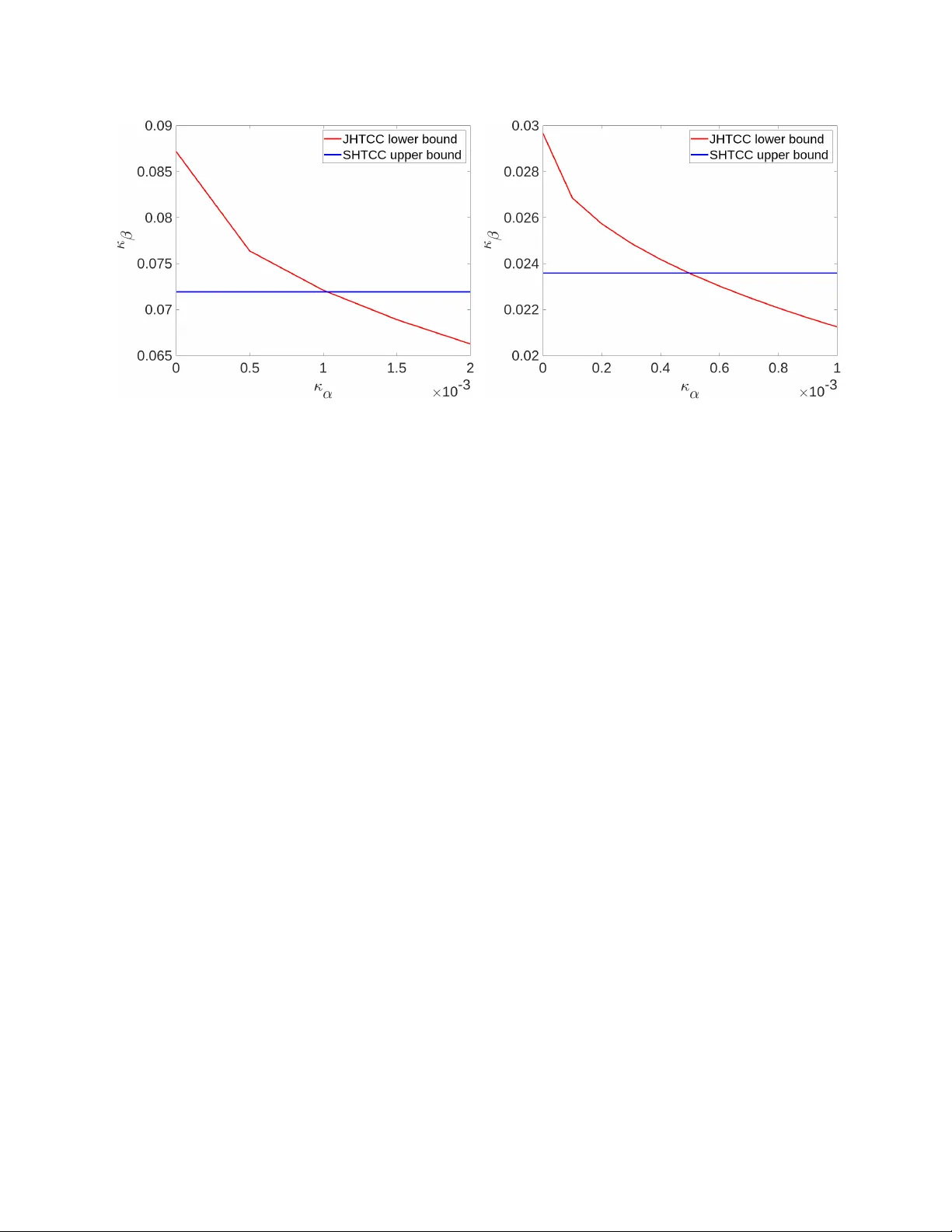
1 Distrib uted Hypothesis T esting o ver a Noisy Channel: Error -e xponents T rade-of f Sreejith Sreekumar and Deniz G ¨ und ¨ uz Abstract A two-terminal distrib uted binary hypothesis testing problem over a noisy channel is studied. The two terminals, called the observer and the decision maker , each has access to n independent and identically distributed samples, denoted by U and V , respectively . The observer communicates to the decision maker o ver a discrete memoryless channel, and the decision maker performs a binary hypothesis test on the joint probability distribution of ( U , V ) based on V and the noisy information received from the observer . The trade-off between the exponents of the type I and type II error probabilities is in vestigated. T wo inner bounds are obtained, one using a separation-based scheme that in volves type-based compression and unequal error -protection channel coding, and the other using a joint scheme that incorporates type-based hybrid coding. The separation-based scheme is shown to recov er the inner bound obtained by Han and Kobayashi for the special case of a rate-limited noiseless channel, and also the one obtained by the authors pre viously for a corner point of the trade-off. Finally , we show via an e xample that the joint scheme achie ves a strictly tighter bound than the separation-based scheme for some points of the error-e xponents trade-off. Index T erms Distributed hypothesis testing, noisy channel, error-exponents, separate hypothesis testing and channel coding, joint source-channel coding, hybrid coding. I . I N T RO D U C T I O N Hypothesis testing (HT), which refers to the problem of choosing between one or more alternatives based on av ailable data, plays a central role in statistics and information theory . Distributed HT (DHT) problems arise in situations where the test data are scattered across multiple terminals, and need to be communicated to a central terminal, called the decision maker , which performs the hypothesis test. The need to jointly optimize the communication scheme and the hypothesis test makes DHT problems much more challenging than their centralized counterparts. Indeed, while an efﬁci ent characterization of the optimal hypothesis test and its asymptotic performance is well known in the centralized setting, thanks to [1]–[5], the same problem in e ven the simplest distrib uted setting remains open, except for some special cases (see [6]–[11]). In this work, we consider a DHT problem with two parties, an observer and a decision maker , such that the former communicates to the latter over a noisy channel. The observer and the decision maker each has access to This work is supported in part by the European Research Council (ERC) through Starting Grant BEACON (agreement #677854). S. Sreekumar was with the Department of Electrical and Electronic Engineering, Imperial College London, at the time of this work. He is now with the School of Electrical and Computer Engineering, Cornell University , Ithaca, NY 14850, USA (email: sreejithsreekumar@cornell.edu). D. G ¨ und ¨ uz is with the Department of Electrical and Electronic Engineering, Imperial College London, London SW72AZ, UK (e-mail: d.gunduz@imperial.ac.uk). 2 independent and identically distributed (i.i.d.) samples, denoted by U and V , respectively . Based on the information receiv ed from the observer and its own observations V , the decision maker performs a binary hypothesis test on the joint distribution of ( U , V ) . Our goal is to characterize the trade-off between the best achie vable rate of decay (or exponent) of the type I and type II error probabilities with respect to the sample size. W e will refer to this problem as DHT over a noisy channel , and its special instance with the noisy channel replaced by a rate-limited noiseless channel as DHT over a noiseless channel . A. Backgr ound Distributed statistical inference problems were ﬁrst conceiv ed in [12] and the information-theoretic study of DHT ov er a noiseless channel was ﬁrst in vestigated in [6], where the objective is to characterize the Stein’ s exponent κ se (  ) , i.e., the optimal type II error -exponent subject to the type I error probability constrained to be at most  ∈ (0 , 1) . The authors therein established a multi-letter characterization of this quantity including a strong con verse, which shows that κ se (  ) is independent of  . Furthermore, a single-letter characterization of κ se (  ) is obtained for a special case of HT known as testing against independence (T AI), in which the joint distribution factors as a product of the mar ginal distributions under the alternative hypothesis. Improved lower bounds on κ se (  ) were subsequently obtained in [7], [8], respectively , and the strong con verse was extended to zero-rate settings [13]. While all the aforementioned works focus on κ se (  ) , the trade-off between the exponents of both the type I and type II error probabilities in the same setting was ﬁrst explored in [14]. In the recent years, there has been a renewed interest in distributed statistical inference problems motiv ated by emerging machine learning applications to be served at the wireless edge, particularly in the context of semantic communications in 5G/6G communication systems [15], [16]. Se veral extensions of the DHT ov er a noiseless channel problem have been studied, such as generalizations to multi-terminal settings [9], [17]–[21], DHT under security or priv acy constraints [22]–[25], DHT with lossy compression [26], interacti ve settings [27], [28], successi ve reﬁnement models [29], and more. Improved bounds ha ve been obtained on the type I and type II error-exponents region [30], [31], and on κ se (  ) for testing correlation between biv ariate standard normal distributions [32]. In the simpler zero- rate communication setting, there has been some progress in terms of second-order optimal schemes [33], geometric interpretation of type I and type II error-exponent re gion [34], and characterization of κ se (  ) for sequential HT [35]. DHT over noisy communication channels with the goal of characterizing κ se (  ) has been considered in [10], [11], [36], [37]. B. Contributions In this work, our objecti ve is to explore the trade-off between the type I and type II error-e xponents for DHT o ver a noisy channel. This problem is a generalization of [14] from noiseless rate-limited channels to noisy channels, and also of [10], [11] from a type I error probability constraint to a positiv e type I error-exponent constraint. Our main contributions can be summarized as follows: (i) W e obtain an inner bound (Theorem 1) on the error-e xponents trade-off by using a separate HT and channel coding scheme (SHTCC) that is a combination of a type-based (type here refers to the empirical probability 3 distribution of a sequence, see [38]) quantize-bin strategy and unequal error-protection scheme of [39]. This result is shown to recover the bounds established in [10], [14]. Furthermore, we ev aluate Theorem 1 for two important instances of DHT , namely T AI and its opposite, i.e., testing against dependence (T AD) in which the joint distribution under the null hypothesis factors as a product of marginal distributions. (ii) W e also obtain a second inner bound (Theorem 2) on the error-e xponents trade-off by using a joint HT and channel coding scheme (JHTCC) based on hybrid coding [40]. Subsequently , we show via an example that the JHTCC scheme strictly outperforms the SHTCC scheme for some points on the error-exponent trade-off. While the abov e schemes are inspired from those in [10], which have been proposed with the goal of maximizing the type II error-e xponent, novel modiﬁcations in its design and analysis are required when considering both of the error -exponents. More speciﬁcally , the schemes presented here perform separate quantization-binning or hybrid coding on each individual source sequence type at the observer/encoder (as opposed to a typical ball in [10]) with the corresponding rev erse operation implemented at the decision-maker/decoder . This necessitates a different analysis to compute the probabilities of the various error events contributing to the overall error-e xponents. W e ﬁnally mention that the DHT problem considered here was recently in vestigated in [41], where an inner bound on the error-e xponents trade-off (Theorem 2 in [41]) is obtained using a combination of a type-based quantization scheme and unequal error protection scheme of [42] with two special messages. A qualitative comparison between Theorem 2 and Theorem 2 in [41] seems to suggest that the JHTCC scheme here uses a stronger decoding rule depending jointly on the source-channel statistics. In comparison, the metric used at the decoder for the scheme in [41] factors as the sum of two metrics, one which depends only on the source statistics, and the other which depends only on the channel statistics. Importantly , this hints that the inner bound achieved by JHTCC scheme is not subsumed by that in [41]. That said, a direct computational comparison appears dif ﬁcult, as e valuating the latter requires optimization over se veral parameters as mentioned in the last paragraph of [41]. C. Or ganization The remainder of the paper is organized as follo ws. Section II formulates the operational problem along with the required deﬁnitions. The main results are presented in Section III. The proofs are furnished in Section IV. Finally , concluding remarks are giv en in Section V. I I . P R E L I M I NA R I E S A. Notation W e use the following notation. All logarithms are with respect to the natural base e . N , R , R ≥ 0 , and ¯ R denotes the set of natural, real, non-negati ve real and extended real numbers, respectively . For a, b ∈ R ≥ 0 , [ a : b ] := { n ∈ N : a ≤ n ≤ b } and [ b ] := [1 : b ] . Calligraphic letters, e.g., X , denote sets, while X c and |X | stands for its complement and cardinality , respectiv ely . For n ∈ N , X n denotes the n -fold Cartesian product of X , and x n = ( x 1 , · · · , x n ) denotes an element of X n . Bold-face letters denote vectors or sequences, e.g., x for x n ; its length n will be clear from the context. For i, j ∈ N such that i ≤ j , x j i := ( x i , x i +1 , · · · , x j ) , the subscript is omitted when i = 1 . 1 A denotes the indicator of set A . For a real sequence { a n } n ∈ N , a n ( n ) − − → b stands for 4 lim n →∞ a n = b , while a n & b denotes lim n →∞ a n ≥ b . Similar notations apply for other inequalities. O ( · ) , Ω( · ) and o ( · ) denote standard asymptotic notations. Random variables and their realizations are denoted by uppercase and lowercase letters, respecti vely , e.g., X and x . Similar con ventions apply for random vectors and their realizations. The set of all probability mass functions (PMFs) on a ﬁnite set X is denoted by P ( X ) . The joint PMF of two discrete random variables X and Y is denoted by P X Y ; the corresponding marginals are P X and P Y . The conditional PMF of X giv en Y is represented by P X | Y . Expressions such as P X Y = P X P Y | X are to be understood as pointwise equality , i.e., P X Y ( x, y ) = P X ( x ) P Y | X ( y | x ) , for all ( x, y ) ∈ X × Y . When the joint distribution of a triple ( X, Y , Z ) factors as P X Y Z = P X Y P Z | X , these variables form a Markov chain X − Y − Z . If the entries of X n are drawn in an i.i.d. manner , i.e., if P X n ( x ) = Q n i =1 P X ( x i ) , ∀ x ∈ X n , then the PMF P X n is denoted by P ⊗ n X . Similarly , if P Y n | X n ( y | x ) = Q n i =1 P Y | X ( y i | x i ) for all ( x , y ) ∈ X n × Y n , then we write P ⊗ n Y | X for P Y n | X n . The conditional product PMF gi ven a ﬁxed x ∈ X n is designated by P ⊗ n Y | X ( ·| x ) . The probability measure induced by a PMF P is denoted by P P . The corresponding expectation is designated by E P . The type or empirical PMF of a sequence x ∈ X n is designated by P x , i.e., P x ( x ) := 1 n P n i =1 1 { x i = x } . The set of n -length sequences x ∈ X n of type P X is T n ( P X , X n ) := { x ∈ X n : P x = P X } . Whenev er the underlying alphabet X n is clear from the context, T n ( P X , X n ) is simpliﬁed to T n ( P X ) . The set of all possible types of n - length sequences x ∈ X n is T ( X n ) :=  P X ∈ P ( X ) :   T n ( P X , X n )   ≥ 1  . Similar notations are used for larger combinations, e.g., P xy , T n ( P X Y , X × Y ) and T ( X n × Y n ) . For a giv en x ∈ T n ( P X , X n ) and a conditional PMF P Y | X , T n ( P Y | X , x ) := { y ∈ Y n : ( x , y ) ∈ T n ( P X Y , X n × Y n ) } stands for the P Y | X -conditional type class of x . For PMFs P , Q ∈ P ( X ) , the K ullback–Leibler (KL) div ergence between P and Q is D ( P || Q ) := P x ∈X P ( x ) log  P ( x ) /Q ( x )  . The conditional KL diver gence between P Y | X and Q Y | X giv en P X is D  P Y | X || Q Y | X   P X  := P x ∈X P X ( x ) D  P Y | X ( ·| x ) || Q Y | X ( ·| x )  . The mutual information and entropy terms are denoted by I P ( · ) and H P ( · ) , respectively , where P denotes the PMF of the relev ant random variables. When the PMF is clear from the context, the subscript is omitted. For ( x , y ) ∈ X n × Y n , the empirical conditional entropy of y given x is H e ( y | x ) := H P ( ˜ Y | ˜ X ) , where P ˜ X ˜ Y = P xy . For a giv en function f : Z → R and a random variable Z ∼ P Z , the log-moment generating function of Z with respect to f is ψ P Z ,f ( λ ) := log E P Z [ e λf ( Z ) ] whenev er the expectation exists. Finally , let ψ ∗ P Z ,f ( θ ) := sup λ ∈ R θ λ − ψ P Z ,f ( λ ) , (1) denote the rate function (see, e.g., Deﬁnition 15.5 in [43]). B. Pr oblem F ormulation Let U , V , X and Y be ﬁnite sets, and n ∈ N . The DHT over a noisy channel setting is depicted in Figure 1. Herein, the observ er and the decision maker observ e n i.i.d. samples, denoted by u and v , respectively . Based on its observations u , the observer outputs a sequence x ∈ X n as the channel input sequence 1 . The discrete memoryless 1 In our problem formulation, we assume that the ratio of the number of channel uses to the number of data samples, termed the bandwidth ratio, is 1. Howe ver , the results easily generalize to arbitrary bandwidth ratios. 5 Fig. 1: DHT ov er a noisy channel. The observer observes an n -length i.i.d. sequence U , and transmits X ov er the DMC P ⊗ n Y | X . Based on the channel output Y and the n -length i.i.d. sequence V , the decision maker performs a binary HT to determine whether ( U , V ) ∼ P ⊗ n U V or ( U , V ) ∼ Q ⊗ n U V . channel (DMC) with transition kernel P Y | X produces a sequence y ∈ Y n according to the probability law P ⊗ n Y | X ( ·| x ) as its output. W e will assume that P Y | X ( ·| x )  P Y | X ( ·| x 0 ) , ∀ ( x, x 0 ) ∈ X 2 , where P  Q indicates absolute continuity of P with respect to Q . Based on its observations, y and v , the decision maker performs binary HT on the joint probability distribution of ( U , V ) with the null ( H 0 ) and alternativ e ( H 1 ) hypotheses giv en by H 0 : ( U , V ) ∼ P ⊗ n U V , H 1 : ( U , V ) ∼ Q ⊗ n U V . The decision maker outputs ˆ h ∈ ˆ H := { 0 , 1 } as the decision of the hypothesis test, where 0 and 1 denote H 0 and H 1 , respectively . A length- n DHT code c n is a pair of functions ( f n , g n ) , where (i) f n : U n → P ( X n ) denotes the encoding function, and (ii) g n : V n × Y n → ˆ H denotes a deterministic decision function 2 speciﬁed by an acceptance region (for null hypothesis H 0 ) A n ⊆ V n × Y n as g n ( v , y ) = 1 − 1 { ( v , y ) ∈A n } , ∀ ( v , y ) ∈ V n × Y n . A code c n = ( f n , g n ) induces the joint PMFs P ( c n ) UVXY ˆ H and Q ( c n ) UVXY ˆ H under the null and alternative hypotheses, respectiv ely , where P ( c n ) UVXY ˆ H ( u , v , x , y , ˆ h ) := P ⊗ n U V ( u , v ) f n ( x | u ) P ⊗ n Y | X ( y | x ) 1  g n ( v , y )= ˆ h  , (3) and Q ( c n ) UVXY ˆ H ( u , v , x , y , ˆ h ) := Q ⊗ n U V ( u , v ) f n ( x | u ) P ⊗ n Y | X ( y | x ) 1  g n ( v , y )= ˆ h  , (4) respectiv ely . For a given code c n , the type I and type II error probabilities are α n ( c n ) := P P ( c n ) ( ˆ H = 1) and β n ( c n ) := P Q ( c n ) ( ˆ H = 0) respectiv ely . The following deﬁnition formally states the error-exponents trade-off we aim to characterize. Deﬁnition 1 ( Error -exponent region ) . An err or-e xponent pair ( κ α , κ β ) ∈ R 2 ≥ 0 is said to be achievable if ther e 2 There is no loss in generality in restricting our attention to a deterministic decision function for the objective of characterizing the error- exponents trade-off in HT (for example, see [24, Lemma 3]). 6 exists a sequence of codes { c n } n ∈ N such that lim inf n →∞ − 1 n log α n ( c n ) ≥ κ α , (5a) lim inf n →∞ − 1 n log β n ( c n ) ≥ κ β . (5b) The err or-exponent re gion ¯ R is the closure of the set of all achievable error -exponent pairs ( κ α , κ β ) . Set R := {  κ α , κ ( κ α )  : κ α ∈ (0 , κ ? α ) } , where κ ? α = inf { κ α : κ ( κ α ) = 0 } and κ ( κ α ) := sup { κ β : ( κ α , κ β ) ∈ ¯ R} . W e are interested in a computable characterization of R , which pertains to the region of positi ve error-exponents (i.e., excluding the boundary points corresponding to Stein’ s exponent). T o this end, we present two inner bounds on R below . I I I . M A I N R E S U LT S In this section, we obtain two inner bounds on R , ﬁrst using a separation-based scheme which performs independent HT and channel coding, termed the SHTCC scheme, and the second via a joint HT and channel coding scheme that uses hybrid coding for communication between the observer and the decision maker . A. Inner Bound on R via SHTCC Scheme Let S = X and P S X Y = P S X P Y | X be a PMF under which S − X − Y forms a Markov chain. For x ∈ X , set Λ x,P S XY ( y ) := log  P Y | X = x ( y ) /P Y | S = x ( y )  and E sp ( P S X , θ ) := X s ∈S P S ( s ) ψ ∗ P Y | S = s , Λ s,P S XY ( θ ) , where the rate function ψ ∗ is deﬁned in (1). For a ﬁxed P S X and R ≥ 0 , let E ex ( R, P S X ) := max ρ ≥ 1 − ρR − ρ log X s,x, ˜ x P S ( s ) P X | S ( x | s ) P X | S ( ˜ x | s )  X y  P Y | X ( y | x ) P Y | X ( y | ˜ x )  1 2  1 ρ ! , denote the expurg ated exponent [44] [38]. Let W be a ﬁnite set and F denote the set of all continuous map- pings from P ( U ) to P ( W |U ) , where P ( W |U ) is the set of all conditional distributions P W | U . Set θ l ( P S X ) := P s ∈S P S ( s ) D  P Y | S = s || P Y | X = s  , θ u ( P S X ) := P s ∈S P S ( s ) D  P Y | X = s || P Y | S = s  , and Θ( P S X ) :=  − θ l ( P S X ) , θ u ( P S X )  . Denote an arbitrary element of F × R ≥ 0 × P ( S × X ) × Θ( P S X ) by ( ω , R, P S X , θ ) , and set L ( κ α ) :=      ( ω , R, P S X , θ ) : ζ ( κ α , ω ) − ρ ( κ α , ω ) ≤ R < I P ( X ; Y | S ) , P S X Y = P S X P Y | X min { E sp ( P S X , θ ) , E ex ( R, P S X ) , E b ( κ α , ω , R ) } ≥ κ α      , ˆ L ( κ α , ω ) :=  P ˆ U ˆ V ˆ W : D  P ˆ U ˆ V ˆ W || P U V ˆ W  ≤ κ α , P ˆ W | ˆ U = ω ( P ˆ U ) , P U V ˆ W = P U V P ˆ W | ˆ U  , (6a) E b ( κ α , ω , R ) :=      R − ζ ( κ α , ω ) + ρ ( κ α , ω ) , if 0 ≤ R < ζ ( κ α , ω ) , ∞ , otherwise , ζ ( κ α , ω ) := max P ˆ U ˆ W : ∃ P ˆ V ,P ˆ U ˆ V ˆ W ∈ ˆ L ( κ α ,ω ) I P ( ˆ U ; ˆ W ) , (6b) 7 ρ ( κ α , ω ) := min P ˆ V ˆ W : ∃ P ˆ U ,P ˆ U ˆ V ˆ W ∈ ˆ L ( κ α ,ω ) I P ( ˆ V ; ˆ W ) , (6c) E 1 ( κ α , ω ) := min ( P ˜ U ˜ V ˜ W ,Q ˜ U ˜ V ˜ W ) ∈T 1 ( κ α ,ω ) D ( P ˜ U ˜ V ˜ W || Q ˜ U ˜ V ˜ W ) , E 2 ( κ α , ω , R ) :=        min ( P ˜ U ˜ V ˜ W ,Q ˜ U ˜ V ˜ W ) ∈T 2 ( κ α ,ω ) D ( P ˜ U ˜ V ˜ W || Q ˜ U ˜ V ˜ W ) + E b ( κ α , ω , R ) , if R < ζ ( κ α , ω ) , ∞ , otherwise , E 3 ( κ α , ω , R, P S X ) :=                      min ( P ˜ U ˜ V ˜ W ,Q ˜ U ˜ V ˜ W ) ∈T 3 ( κ α ,ω ) D ( P ˜ U ˜ V ˜ W || Q ˜ U ˜ V ˜ W ) + E b ( κ α , ω , R ) + E ex ( R, P S X ) , if R < ζ ( κ α , ω ) , min ( P ˜ U ˜ V ˜ W ,Q ˜ U ˜ V ˜ W ) ∈T 3 ( κ α ,ω ) D ( P ˜ U ˜ V ˜ W || Q ˜ U ˜ V ˜ W ) + ρ ( κ α , ω ) + E ex ( R, P S X ) , otherwise , E 4 ( κ α , ω , R, P S X , θ ) :=                        min P ˆ V : P ˆ U ˆ V ˆ W ∈ ˆ L ( κ α ,ω ) D ( P ˆ V || Q V ) + E b ( κ α , ω , R ) + E m ( P S X , θ ) − θ , if R < ζ ( κ α , ω ) , min P ˆ V : P ˆ U ˆ V ˆ W ∈ ˆ L ( κ α ,ω ) D ( P ˆ V || Q V ) + ρ ( κ α , ω ) + E m ( P S X , θ ) − θ , otherwise , T 1 ( κ α , ω ) :=    ( P ˜ U ˜ V ˜ W , Q ˜ U ˜ V ˜ W ) : P ˜ U ˜ W = P ˆ U ˆ W , P ˜ V ˜ W = P ˆ V ˆ W , Q ˜ U ˜ V ˜ W := Q U V P ˜ W | ˜ U for some P ˆ U ˆ V ˆ W ∈ ˆ L ( κ α , ω )    , (6d) T 2 ( κ α , ω ) :=    ( P ˜ U ˜ V ˜ W , Q ˜ U ˜ V ˜ W ) : P ˜ U ˜ W = P ˆ U ˆ W , P ˜ V = P ˆ V , H P ( ˜ W | ˜ V ) ≥ H P ( ˆ W | ˆ V ) , Q ˜ U ˜ V ˜ W := Q U V P ˜ W | ˜ U for some P ˆ U ˆ V ˆ W ∈ ˆ L ( κ α , ω )    , T 3 ( κ α , ω ) :=    ( P ˜ U ˜ V ˜ W , Q ˜ U ˜ V ˜ W ) : P ˜ U ˜ W = P ˆ U ˆ W , P ˜ V = P ˆ V , Q ˜ U ˜ V ˜ W := Q U V P ˜ W | ˜ U for some P ˆ U ˆ V ˆ W ∈ ˆ L ( κ α , ω )    . W e have the follo wing lower bound for κ ( κ α ) which translates to an inner bound for R . Theorem 1 (Inner bound via SHTCC scheme) . κ ( κ α ) ≥ κ ? s ( κ α ) , where κ ? s ( κ α ) := max ( ω ,R,P S X ,θ ) ∈ L ( κ α ) min  E 1 ( κ α , ω ) , E 2 ( κ α , ω , R ) , E 3 ( κ α , ω , R, P S X ) , E 4 ( κ α , ω , R, P S X , θ )  . (7) The proof of Theorem 1 is presented in Section IV -A. The SHTCC scheme, which achiev es the error-exponent pair ( κ α , κ ? s ( κ α )) , is a coding scheme analogous to separate source and channel coding for the lossy transmission of a source over a communication channel with correlated side-information at the receiv er [45], howe ver , with the objectiv e of reliable HT . In this scheme, the source samples are ﬁrst compressed to an index, which acts as the message to be transmitted over the channel. But, in contrast to standard communication problems, there is a need to protect certain messages more reliably than others; hence, an unequal error -protection scheme [39], [42] is used. T o describe brieﬂy , the SHTCC scheme in volv es ( i ) the quantization and binning of u sequences, whose type P u is within a κ α -neighborhood (in terms of KL div ergence) of P U , using V as side information at the decision maker for 8 decoding, and ( ii ) unequal error-protection channel coding scheme in [39] for protecting a special message which informs the decision maker that P u lies outside the κ α -neighborhood of P U . The output of the channel decoder is processed by an empirical conditional entropy decoder which recovers the quantization codew ord with the least conditional entropy with V . Since this decoder depends only on the empirical distrib utions of the observations, it is univ ersal and useful in the hypothesis testing context, where multiple distributions are in volved (as was ﬁrst noted in [8]). The various factors E 1 to E 4 in (7) ha ve natural interpretations in terms of e vents that could possibly result in a hypothesis testing error . Speciﬁcally , E 1 and E 2 correspond to the error e vents arising due to quantization and binning, respectively , while E 3 and E 4 correspond to the error ev ents of wrongly decoding an ordinary channel codew ord and special message codew ord, respectiv ely . Remark 1 (Generalization of Han-Kobayashi inner bound) . In [14, Theor em 1], Han and K obayashi obtained an inner bound on R for DHT over a noiseless channel. At a high level, their coding scheme involves type-based quantization of u ∈ U n sequences, whose type P u lies within a κ α -neighbourhood of P U , wher e κ α is the desired type I err or-e xponent. As a cor ollary , Theorem 1 r ecovers the lower bound for κ ( κ α ) obtained in [14] by ( i ) setting E ex ( R, P S X ) , E m ( P S X , θ ) and E m ( P S X , θ ) − θ to ∞ , which hold when the channel is noiseless; and ( ii ) maximizing over the set  ( ω , R, P S X , θ ) ∈ F × R ≥ 0 × P ( S × X ) × Θ( P S X ) : ζ ( κ α , ω ) ≤ R < I P ( X ; Y | S ) , P S X Y := P S X P Y | X  ⊆ L ( κ α ) in (7) . Then, note that the terms E 2 ( κ α , ω , R ) , E 3 ( κ α , ω , R, P S X ) and E 4 ( κ α , ω , R, P S X , θ ) all equal ∞ , and thus the inner bound in Theor em 1 reduces to that given in [14, Theorem 1]. Remark 2 (Improvement via time-sharing) . Since the lower bound on κ ( κ α ) in Theor em 1 is not necessarily concave, a tighter bound can be obtained using the technique of time-sharing similar to [14, Theor em 3]. W e omit its description as it is cumbersome, although straightforwar d. Theorem 1 also recov ers the lower bound for the optimal type II error-e xponent for a ﬁxed type I error probability constraint established in [10, Theorem 2] by letting κ α → 0 . The details are provided in Appendix A. Further , specializing the lower bound in Theorem 1 to the case of T AI, i.e., when Q U V = P U P V , we obtain the following corollary which recovers the optimal type II error-exponent for T AI established in [10, Proposition 7]. Corollary 1 (Inner bound for T AI) . Let P U V ∈ P ( U × V ) be an arbitrary distribution and Q U V = P U P V . Then, κ ( κ α ) ≥ κ ? s ( κ α ) ≥ κ ? i ( κ α ) , (8) wher e κ ? i ( κ α ) := max ( ω ,P S X ,θ ) ∈L ? ( κ α ) min  E i 1 ( κ α , ω ) , E i 2 ( κ α , ω , P S X ) , E i 3 ( κ α , ω , P S X , θ )  , L ? ( κ α ) :=      ( ω , P S X , θ ) ∈ F × P ( S × X ) × Θ( P S X ) : ζ ( κ α , ω ) < I P ( X ; Y | S ) , P S X Y := P S X P Y | X , min { E sp ( P S X , θ ) , E ex ( ζ ( κ α , ω ) , P S X ) } ≥ κ α      , (9) E i 1 ( κ α , ω ) := min P ˆ V ˆ W : ∃ P ˆ U ˆ V ˆ W ∈ ˆ L ( κ α ,ω ) I P ( ˆ V ; ˆ W ) + D ( P ˆ V || P V ) , 9 E i 2 ( κ α , ω , P S X ) := ρ ( κ α , ω ) + E ex  ζ ( κ α , ω ) , P S X  , E i 3 ( κ α , ω , P S X , θ ) := ρ ( κ α , ω ) + E sp ( P S X , θ ) − θ , and, ˆ L ( κ α , ω ) , ζ ( κ α , ω ) and ρ ( κ α , ω ) are deﬁned in (6a) , (6b) and (6c) , r espectively . In particular , lim κ α → 0 κ ( κ α ) = κ ? s (0) = κ ? i (0) = max P W | U : I P ( U ; W ) ≤ C ( P Y | X ) , P U V W = P U V P W | U I P ( V ; W ) , (10) wher e |W | ≤ |U | + 1 and C ( P Y | X ) denotes the capacity of the channel P Y | X . The proof of Corollary 1 is giv en in Section IV -B. Its achiev ability follows from a special case of the SHTCC scheme without binning at the encoder . Next, we consider testing a gainst dependence (T AD) for which Q U V is an arbitrary joint distribution and P U V = Q U Q V . Theorem 1 specialized to T AD gives the following corollary . Corollary 2 (Inner bound for T AD) . Let Q U V ∈ P ( U × V ) be an arbitrary distribution and P U V = Q U Q V . Then, κ ( κ α ) ≥ κ ? s ( κ α ) = κ ? d ( κ α ) := max ( ω ,P S X ,θ ) ∈L ? ( κ α ) min  E d 1 ( κ α , ω ) , E d 2 ( κ α , ω , P S X ) , E d 3 ( P S X , θ )  , (11) wher e E d 1 ( κ α , ω ) := min ( P ˜ U ˜ V ˜ W ,Q ˜ U ˜ V ˜ W ) ∈T 1 ( κ α ,ω ) D ( P ˜ U ˜ V ˜ W || Q ˜ U ˜ V ˜ W ) ≥ min ( P ˆ V ˆ W ,Q V ˆ W ): P ˆ U ˆ V ˆ W ∈ ˆ L ( κ α ,ω ) , Q U V ˆ W = Q U V P ˆ W | ˆ U D ( P ˆ V ˆ W || Q V ˆ W ) , E d 2 ( κ α , ω , P S X ) := E ex ( ζ ( κ α , ω ) , P S X ) , E d 3 ( P S X , θ ) := E sp ( P S X , θ ) − θ , and, ˆ L ( κ α , ω ) , T 1 ( κ α , ω ) and L ? ( κ α ) are given in (6a) , (6d) and (9) , r espectively . In particular , lim κ α → 0 κ ( κ α ) ≥ κ ? s (0) = κ ? d (0) ≥ κ ? T AD , (12) wher e κ ? T AD = max ( P W | U ,P S X ): I Q ( W ; U ) ≤ I P ( X ; Y | S ) , Q U V W = Q U V P W | U , P S XY = P S X P Y | X min  D ( Q V Q W || Q V W ) , E ex ( I Q ( U ; W ) , P S X ) , θ l ( P S X )  , and |W | ≤ |U | + 1 . The proof of Corollary 2 is gi ven in Section IV -C. Note that the expression for κ ? s ( κ α ) given in (11) is relativ ely simpler to compute compared to that in Theorem 1. This will be handy in showing that the JHTCC scheme strictly outperforms the SHTCC scheme, which we highlight via an example in Section III-C below . 10 B. Inner Bound via JHTCC Scheme It is well kno wn that joint source-channel coding schemes offer advantages over separation-based coding schemes in several information theoretic problems, such as the transmission of correlated sources over a multiple-access channel [40], [46] and the error-exponent in the lossless or lossy transmission of a source ov er a noisy channel [42], [47]. Recently , it is shown via an example in [10] that joint schemes also achiev e a strictly larger type II error-e xponent in DHT problems compared to a separation-based scheme in some scenarios. Motiv ated by this, we present an inner bound on R using a generalization of the JHTCC scheme in [10]. Let W and S be arbitrary ﬁnite sets, and F 0 denote the set of all continuous mappings from P ( U × S ) to P ( W | U × S ) , where P ( W | U × S ) is the set of all conditional distributions P W | U S . Let  P S , ω 0 ( · , P S ) , P X | U S W , P X 0 | U S  denote an arbitrary element of P ( S ) × F 0 × P ( X |U × S × W ) × P ( X |U × S ) , and deﬁne L h ( κ α ) :=  P S , ω 0 ( · , P S ) , P X | U S W , P X 0 | U S  : E 0 b ( κ α , ω 0 , P S , P X | U S W ) ≥ κ α  , ˆ L h ( κ α , ω 0 , P S , P X | U S W ) :=      ( P ˆ U ˆ V ˆ W ˆ Y S : D ( P ˆ U ˆ V ˆ W ˆ Y | S || P U V ˆ W Y | S | P S ) ≤ κ α , P S U V ˆ W X Y := P S P U V P ˆ W | ˆ U S P X | U S W P Y | X , P ˆ W | ˆ U S = ω 0 ( P ˆ U , P S )      , E 0 b ( κ α , ω 0 , P S , P X | U S W ) := ρ 0 ( κ α , ω 0 , P S , P X | U S W ) − ζ 0 q ( κ α , ω 0 , P S ) , ζ 0 ( κ α , ω 0 , P S ) := max P ˆ U ˆ W S : ∃ P ˆ V ˆ Y s.t. P ˆ U ˆ V ˆ W ˆ Y S ∈ ˆ L h ( κ α ,ω 0 ,P S ,P X | U SW ) I P ( ˆ U ; ˆ W | S ) , ρ 0 ( κ α , ω 0 , P S , P X | U S W ) := min P ˆ V ˆ W ˆ Y S : ∃ P ˆ U s.t. P ˆ U ˆ V ˆ W ˆ Y S ∈ ˆ L h ( κ α ,ω 0 ,P S ,P X | U SW ) I P ( ˆ Y , ˆ V ; ˆ W | S ) , E 0 1 ( κ α , ω 0 ) := min ( P ˜ U ˜ V ˜ W ˜ Y S ,Q ˜ U ˜ V ˜ W ˜ Y S ) ∈T 0 1 ( κ α ,ω 0 ) D ( P ˜ U ˜ V ˜ W ˜ Y | S || Q ˜ U ˜ V ˜ W ˜ Y | S | P S ) , E 0 2 ( κ α , ω 0 , P S , P X | U S W ) := min ( P ˜ U ˜ V ˜ W ˜ Y S ,Q ˜ U ˜ V ˜ W ˜ Y S ) ∈T 0 2 ( κ α ,ω 0 ,P S ,P X | U SW ) D ( P ˜ U ˜ V ˜ W ˜ Y | S || Q ˜ U ˜ V ˜ W ˜ Y | S | P S ) + E 0 b ( κ α , ω 0 , P S , P X | U S W ) , E 0 3 ( κ α , ω 0 , P S , P X | U S W , P X 0 | U S ) := min P ˆ V ˆ Y S : P ˆ U ˆ V ˆ W ˆ Y S ∈ ˆ L h ( κ α ,ω 0 ,P S ,P X | U SW ) D ( P ˆ V ˆ Y | S || Q V Y 0 | S | P S ) + E 0 b ( κ α , ω 0 , P S , P X | U S W ) , Q S U V X 0 Y 0 := P S Q U V P X 0 | U S P Y 0 | X 0 , P Y 0 | X 0 := P Y | X , T 0 1 ( κ α , ω 0 , P S , P X | U S W ) :=          ( P ˜ U ˜ V ˜ W ˜ Y S , P ˜ U ˜ W S = P ˆ U ˆ W S , P ˜ V ˜ W ˜ Y S = P ˆ V ˆ W ˆ Y S , Q ˜ U ˜ V ˜ W ˜ Y S ) : Q S ˜ U ˜ V ˜ W ˜ X ˜ Y := P S Q U V P ˜ W | ˜ U S P X | U S W P Y | X for some P ˆ U ˆ V ˆ W ˆ Y S ∈ ˆ L h ( κ α , ω 0 , P S , P X | U S W )          , 11 T 0 2 ( κ α , ω 0 , P S , P X | U S W ) :=                ( P ˜ U ˜ V ˜ W ˜ Y S , P ˜ U ˜ W S = P ˆ U ˆ W S , P ˜ V ˜ Y S = P ˆ V ˆ Y S , Q ˜ U ˜ V ˜ W ˜ Y S ) : H P ( ˜ W | ˜ V , ˜ Y , S ) ≥ H P ( ˆ W | ˆ V , ˆ Y , S ) , Q S ˜ U ˜ V ˜ W ˜ X ˜ Y := P S Q U V P ˜ W | ˜ U S P X | U S W P Y | X for some P ˆ U ˆ V ˆ W ˆ Y S ∈ ˆ L h ( κ α , ω 0 , P S , P X | U S W )                . Then, we have the following result. Theorem 2 (Inner bound via JHTCC scheme) . κ ( κ α ) ≥ max { κ ? h ( κ α ) , κ ? u ( κ α ) } , wher e κ ? h ( κ α ) := max ( P S ,ω 0 ,P X | U SW ,P X 0 | U S ) ∈ L h ( κ α ) min n E 0 1 ( κ α , ω 0 ) , E 0 2 ( κ α , ω 0 , P S , P X | U S W ) , E 0 3 ( κ α , ω 0 , P S , P X | U S W , P X 0 | U S ) o , κ ? u ( κ α ) := max ( P S ,P X | U S ) ∈P ( S ) ×P ( X |S ×U ) κ u ( κ α , P S , P X | U S ) , κ u ( κ α , P S , P X | U S ) := min P S P ˆ V ˆ Y : D  P ˆ V ˆ Y | S || P V Y | S | P S  ≤ κ α D  P ˆ V ˆ Y | S || Q V Y | S | P S  , P S U V X Y = P S P U V P X | U S P Y | X and Q S U V X Y = P S Q U V P X | U S P Y | X . The proof of Theorem 2 is given in Section IV -D, and utilizes a generalization of hybrid coding scheme [40] to achiev e the stated inner bound. Speciﬁcally , the error-e xponent pair  κ α , κ ? h ( κ α )  is achiev ed using type-based hybrid coding, while  κ α , κ ? u ( κ α )  is realized by uncoded transmission, in which the channel input X is generated as the output of a DMC P X | U with input U (along with time sharing). In standard hybrid coding, the source sequence is ﬁrst quantized via joint typicality and the channel input is then chosen as a function of both the original source sequence and its quantization. At the decoder , the quantized codew ord is ﬁrst recovered using the channel output and side information via joint typicality decoding, and an estimate of the source sequence is output as a function of the channel output and recovered codeword. The quantization part forms the digital part of the scheme, while the use of the source sequence for encoding and channel output for decoding comprises the analog part. The scheme deriv es its name from these joint hybrid digital-analog operations. In the HT context considered here, the aforementioned source quantization is replaced by a type-based quantization at the encoder , and the joint typicality decoder is replaced by a univ ersal empirical conditional entropy decoder . W e note that Theorem 2 recov ers the lower bound on the optimal type II error-e xponent prov ed in Theorem 5 in [10]. The details are provided in Appendix B. Next, we provide a comparison between the SHTCC and JHTCC bounds via an example as mentioned earlier . C. Comparison of Inner Bounds W e compare the inner bounds established in Theorem 1 and Theorem 2 for a simple setting of T AD o ver a BSC. For this purpose, we will use the inner bound κ ? d ( κ α ) stated in Corollary 2 and κ ? u ( κ α ) that is achie ved by uncoded 12 (a) p = 0 . 25 and q = 0 (b) p = 0 . 35 and q = 0 Fig. 2: Comparison of the error-e xponents trade-off achieved by the SHTCC and JHTCC schemes for T AD over a BSC in Example 1 with parameters p = 0 . 25 , q = 0 for Figure 2a and p = 0 . 35 , q = 0 for Figure 2b. The red curve sho ws ( κ α , κ ? u ( κ α )) pairs achie ved by uncoded transmission while the blue line plots ( κ α , E ex (0)) . The joint scheme clearly achie ves a better error -exponent trade-of f for values of κ α below a threshold which depends on the transition kernel of the channel. In particular, a more uniform channel results in a lesser threshold. transmission. Our objecti ve is to illustrate that the JHTCC scheme achie ves a strictly tighter bound on R compared to the SHTCC scheme, at least for some points of the trade-off. Example 1 (Comparison of inner bounds) . Let p, q ∈ [0 , 0 . 5] , U = V = X = Y = S = { 0 , 1 } , Q U V =   q 0 . 5 − q 0 . 5 − q q   , P Y | X =   1 − p p p 1 − p   , and P U V = Q U Q V . A comparison of the inner bounds achieved by the SHTCC and JHTCC schemes for the above example are shown in Figures 2 and 3, where we plot the error-exponents trade-of f achieved by uncoded transmission (a lower bound for the JHTCC scheme), and the expurgated exponent at a zero rate: E ex (0) := max P S X ∈P ( S ×X ) E ex ( P S X , 0) = − 0 . 25 log (4 p (1 − p )) , which is an upper bound on κ ? d ( κ α ) for any κ α ≥ 0 . T o compute E ex (0) , we used the closed-form expression for E ex ( · ) giv en in Problem 10.26(c) in [38]. Clearly , it can be seen that the JHTCC scheme outperforms SHTCC scheme for κ α below a threshold, which depends on the source and channel distributions. In particular , the threshold below which improv ement is seen is reduced when the channel or the source becomes more uniform. The former behavior can be seen directly by comparing the subplots in Figures 2 and 3, while the latter can be noted by comparing Figure 2a with Figure 3a, or Figure 2b with Figure 3b . 13 (a) p = 0 . 25 and q = 0 . 05 (b) p = 0 . 35 and q = 0 . 05 Fig. 3: Comparison of the error-e xponents trade-off achiev ed by the SHTCC and JHTCC schemes for Example 1 with parameters p = 0 . 25 , q = 0 . 05 for Figure 3a and p = 0 . 35 , q = 0 . 05 for Figure 3b. The JHTCC scheme improv es over the separation based scheme for small values of κ α ; ho wever , the region of improvement is reduced compared to Figure 2 as the source is more uniformly distributed. I V . P RO O F S A. Pr oof of Theorem 1 W e will show the achiev ability of the error-e xponent pair ( κ α , κ ? s ( κ α )) by constructing a suitable ensemble of HT codes, and sho wing that the expected type I and type II error probabilities (over this ensemble) satisfy (5) for the pair ( κ α , κ ? s ( κ α )) . Then, an expurgation argument [44] will be used to show the existence of a HT code that satisﬁes (5) for the same error-exponent pair , thus showing that ( κ α , κ ? s ( κ α )) ∈ R as desired. Let n ∈ N , |W | < ∞ , κ α > 0 , ( ω , R, P S X , θ ) ∈ L ( κ α ) , R 0 := ζ ( κ α , ω ) , and η > 0 be a small number . Also, suppose R ≥ 0 satisfy ζ ( κ α , ω ) − ρ ( κ α , ω ) ≤ R < I P ( X ; Y | S ) , (13) where ζ ( κ α , ω ) and ρ ( κ α , ω ) are deﬁned in (6b) and (6c), respectively . The SHTCC scheme is as follo ws: Encoding: The observer’ s encoder is composed of two stages, a sour ce encoder followed by a channel encoder . Source encoder: The source encoding comprises of a quantization scheme followed by binning to reduce the rate if necessary . Quantization codebook: Let D n ( P U , η ) :=  P ˆ U ∈ T ( U n ) : D ( P ˆ U || P U ) ≤ κ α + η  . (14) Consider some ordering on the types in D n ( P U , η ) and denote the elements as P ˆ U i for i ∈  |D n ( P U , η ) |  . For each 14 type P ˆ U i ∈ D n ( P U , η ) , i ∈  |D n ( P U , η ) |  , choose a joint type variable P ˆ U i ˆ W i ∈ T ( U n × W n ) such that D  P ˆ W i | ˆ U i || P W i | U   P ˆ U i  ≤ η 3 , (15a) I P  ˆ U i ; ˆ W i  ≤ R 0 + η 3 , (15b) where P W i | U = ω ( P ˆ U i ) . Note that this is always possible for n sufﬁciently large by deﬁnition of R 0 . Let D n ( P U W , η ) :=  P ˆ U i ˆ W i : i ∈  |D n ( P U , η ) |  , (16a) R 0 i := I P  ˆ U i ; ˆ W i  + ( η / 3) , i ∈  |D n ( P U , η ) |  , (16b) M 0 i := " 1 + i − 1 X k =1 e nR 0 k : i X k =1 e nR 0 k # , (16c) and B W,n =  W ( j ) , 1 ≤ j ≤ P |D n ( P U ,η ) | i =1 |M 0 i |  denote a random quantization codebook such that the codeword W ( j ) ∼ Unif  T n ( P ˆ W i )  , if j ∈ M 0 i for some i ∈  |D n ( P U , η ) |  . Denote a realization of B W,n by B W,n =  w ( j ) ∈ W n , 1 ≤ j ≤ P |D n ( P U ,η ) | i =1 |M 0 i |  . Quantization scheme: For a giv en codebook B W,n and u ∈ T n  P ˆ U i  such that P ˆ U i ∈ D n ( P U , η ) for some i ∈  |D n ( P U , η ) |  , let ˜ M  u , B W,n  :=  j ∈ M 0 i : w ( j ) ∈ B W,n , ( u , w ( j )) ∈ T n  P ˆ U i ˆ W i  , P ˆ U i ˆ W i ∈ D n ( P U W , η )  . If | ˜ M ( u , B W,n ) | ≥ 1 , let M 0 ( u , B W,n ) denote an index selected uniformly at random from the set ˜ M ( u , B W,n ) , otherwise, set M 0 ( u , B W,n ) = 0 . Denoting the support of M 0 ( u , B W,n ) by M 0 , we have for sufﬁciently large n that |M 0 | ≤ 1 + |D n ( P U ,η ) | X i =1 e nR 0 i ≤ 1 + |D n ( P U , η ) | e max P ˆ U ˆ W ∈D n ( P U W ,η ) nI ( ˆ U ; ˆ W )+( nη / 3) ≤ e n ( R 0 + η ) , (17) where the last inequality uses (15b) and |D n ( P U , η ) | ≤ ( n + 1) |U | . Binning: If |M 0 | > |M| , then the source encoder performs binning as gi ven belo w . Let R n := log  e nR / |D n ( P U , η ) |  , M i := [1 + ( i − 1) R n : iR n ] , i ∈  |D n ( P U , η ) |  , and M := { 0 } S  ∪ i ∈ [ |D n ( P U ,η ) | ] M i  . Note that e nR n ≥ e nR −|U | log( n +1) . (18) Let f B denote the random binning function such that for each j ∈ M 0 i , f B ( j ) ∼ Unif [ |M i | ] for i ∈  |D n ( P U , η ) |  , and f B (0) = 0 with probability one. Denote a realization of f B ( j ) by f b , where f b : M 0 → M . Gi ven a codebook B W,n and binning function f b , the source encoder outputs M = f b ( M 0 ( u , B W,n )) for u ∈ U n . If |M 0 | ≤ |M| , then f b is taken to be the identity map (no binning), and in this case, M = M 0 ( u , B W,n ) . Channel codebook: Let B X,n := { X ( m ) ∈ X n , m ∈ M} denote a random channel codebook generated as follows. Without loss of generality (w .l.o.g.), denote the elements of the set S = X as 1 , . . . , |X | . The codeword length n is divided into |S | = |X | blocks, where the length of the ﬁrst block is d P S (1) n e , the second block 15 is d P S (2) n e , so on so forth, and the length of the last block is chosen such that the total length is n . For i ∈ [ |X | ] , let k i := P i − 1 l =1 d P S ( l ) n e + 1 and ¯ k i := P i l =1 d P S ( l ) n e , where the empty sum is deﬁned to be zero. Let s ∈ X n be such that s ¯ k i k i = i , i.e., the elements of s equal i in the i th block for i ∈ [ |X | ] . Let X (0) = s with probability one, and the remaining codew ords X ( m ) , m ∈ M\{ 0 } be constant composition codewords [38] selected such that X ¯ k i k i ( m ) ∼ Unif  T d P S ( i ) n e ( ˆ P X | S ( ·| i ))  , where ˆ P X | S is such that T d P S ( i ) n e  ˆ P X | S ( ·| i )  is non- empty and D ( ˆ P X | S || P X | S | P S ) ≤ η 3 . Denote a realization of B X,n by B X,n := { x ( m ) ∈ X n , m ∈ M} . Note that for m ∈ M\{ 0 } and lar ge n , the code word pair ( x (0) , x ( m )) has joint type (approx) P x (0) x ( j ) = ˆ P S X := P S ˆ P X | S . Channel encoder: For a gi ven B X,n , the channel encoder outputs x = x ( m ) for output m from the source encoder . Denote this map by f B X,n : M → X n . Encoder: Denote by f n : U n → P ( X n ) the encoder induced by all the abov e operations, i.e., f n ( ·| u ) = f B X,n ◦ f b  M 0 ( u , B W,n )  . Decision function: The decision function consists of three parts, a channel decoder , a source decoder and a tester . Channel decoder: The channel decoder ﬁrst performs a Neyman-Pearson test on the channel output y according to ˜ Π θ : Y n → { 0 , 1 } , where ˜ Π θ ( y ) := 1 n X i =1 log  P Y | X ( y i | s i ) P Y | S ( y i | s i )  ≥ nθ ! . (19) If ˜ Π θ ( y ) = 1 , then ˆ M = 0 . Else, for a given B X,n , maximum likelihood (ML) decoding is done on the remaining set of codewords { x ( m ) , m ∈ M\{ 0 }} , and ˆ M is set equal to the ML estimate. Denote the channel decoder induced by the abov e operations by g B X,n , where g B X,n : Y n → M . For a given codebook B X,n , the channel encoder-decoder pair described above induces a distribution P ( B X,n ) XY ˆ M | M ( m, x , y , ˆ m | m ) := 1  f B X,n ( m )= x  P ⊗ n Y | X ( y | x ) 1  ˆ m = g B X,n  . Note that P x (0) x ( m ) = ˆ P S X , Y ∼ Q |X | i =1 P ⊗d P S ( i ) n e Y | X ( ·| i ) for M = 0 and Y ∼ Q |X | i =1 P ⊗d P S ( i ) n e Y | S ( ·| i ) for M = m 6 = 0 . Then, it follows by an application of Proposition 1 proved in Appendix C that for any B X,n and n sufﬁciently large, the Neyman-Pearson test in (19) yields P P ( B X,n )  ˆ M = 0 | M = m  ≤ e − n ( E sp ( P S X ,θ ) − η ) , m ∈ M\{ 0 } , (20a) P P ( B X,n )  ˆ M 6 = 0 | M = 0  ≤ e − n ( E sp ( P S X ,θ ) − θ − η ) . (20b) Moreov er, giv en ˆ M 6 = 0 , a random coding ar gument ov er the ensemble of B n X (see [38, Exercise 10.18, 10.24] and [44]) shows that there exists a deterministic codebook B X,n such that (20) holds, and the ML-decoding described abov e asymptotically achie ves P P ( B X,n )  ˆ M 6 = m | M = m 6 = 0 , ˆ M 6 = 0  ≤ e − n ( E ex ( R,P S X ) − η ) . (21) This deterministic codebook B X,n is used for channel coding. Source decoder: For a given codebook B W,n and inputs ˆ M = ˆ m and V = v , the source decoder ﬁrst decodes for 16 the quantization codeword w ( ˆ m 0 ) (if required) using the empirical conditional entropy decoder, and then declares the output ˆ H of the hypothesis test based on w ( ˆ m 0 ) and v . More speciﬁcally , if binning is not performed, i.e., if |M| ≥ |M 0 | , ˆ M 0 = ˆ m . Otherwise, ˆ M 0 = ˆ m 0 , where ˆ m 0 = 0 if ˆ m = 0 and ˆ m 0 = arg m i n j : f b ( j )= ˆ m H e ( w ( j ) | v ) otherwise. Denote the source decoder induced by the above operations by g B W,n : M × V n → M 0 . T esting and Acceptance region: If ˆ m 0 = 0 , ˆ H = 1 is declared. Otherwise, ˆ H = 0 or ˆ H = 1 is declared depending on whether ( ˆ m 0 , v ) ∈ A n or ( ˆ m 0 , v ) / ∈ A n , respecti vely , where A n denotes the acceptance region for H 0 as speciﬁed next. For a gi ven codebook B W,n , let O m 0 denote the set of u such that the source encoder outputs m 0 , m 0 ∈ M 0 \{ 0 } . For each m 0 ∈ M 0 \{ 0 } and u ∈ O m 0 , let Z m 0 ( u ) = { v ∈ V n : ( w ( m 0 ) , u , v ) ∈ J n ( κ α + η , P W m 0 U V ) } , where J n ( r , P X ) := { x ∈ X n : D ( P x || P X ) ≤ r } , P U V W m 0 := P U V P W m 0 | U and P W m 0 | U = ω ( P u ) . (22) For m 0 ∈ M 0 \{ 0 } , set Z m 0 := { v : v ∈ Z m 0 ( u ) for some u ∈ O m 0 } , and deﬁne the acceptance region for H 0 at the decision maker as A n := ∪ m 0 ∈M 0 \ 0 m 0 × Z m 0 or equiv alently as A e n := ∪ m 0 ∈M 0 \ 0 O m 0 × Z m 0 . Note that A n is the same as the acceptance region for H 0 in [14, Theorem 1]. Denote the decision function induced by g B X,n , g B W,n and A n by g n : Y n × V n → ˆ H . Induced probability distribution: The PMFs induced by a code c n = ( f n , g n ) with respect to codebook B n := ( B W,n , f b , B X,n ) under H 0 and H 1 are P ( B n ,c n ) UV M 0 M XY ˆ M ˆ M 0 ˆ H ( u , v , m 0 , m, x , y , ˆ m, ˆ m 0 , ˆ h ) := P ⊗ n U V ( u , v ) 1 { M 0 ( u , B W,n )= m 0 , f b ( m 0 )= m } P ( B X,n ) XY ˆ M | M ( x , y , ˆ m | m ) 1  g B W,n ( m, v )= ˆ m 0 , ˆ h = 1 { ( ˆ m 0 , v ) ∈A c n }  , Q ( B n ,c n ) UV M 0 M XY ˆ M ˆ M 0 ˆ H ( u , v , m 0 , m, x , y , ˆ m, ˆ m 0 , ˆ h ) := Q ⊗ n U V ( u , v ) 1 { M 0 ( u , B W,n )= m 0 , f b ( m 0 )= m } P ( B X,n ) XY ˆ M | M ( x , y , ˆ m | m ) 1 n g B W,n ( m, v )= ˆ m 0 , ˆ h = 1 { ( ˆ m 0 , v ) ∈A c n } o , respectiv ely . F or simplicity , we will denote the abov e distributions by P ( B n ) and Q ( B n ) . Let B n := ( B W,n , f B , B X,n ) , B n , and µ n denote the random codebook, its support, and the probability measure induced by its random construc- tion, respectively . Also, deﬁne ¯ P P ( B n ) := E µ n  P P ( B n )  and ¯ P Q ( B n ) := E µ n  P Q ( B n )  . Analysis of the type I and type II err or probabilities: W e analyze the type I and type II error probabilities a veraged ov er the random ensemble of quantization and binning codebooks ( B W , f B ) . Then, an expur gation technique [44] guarantees the existence of a sequence of deterministic codebooks {B n } n ∈ N and a code { c n = ( f n , g n ) } n ∈ N that achiev es the lower bound giv en in Theorem 1. T ype I error probability: In the follo wing, random sets where the randomness is induced due to B n will be written using blackboard bold letters, e.g., A n for the random acceptance region for H 0 . Note that a type I error can occur only under the following e vents: 17 (i) E EE := S P ˆ U ∈D n ( P U ,η ) S u ∈T n ( P ˆ U ) E EE ( u ) , where E EE ( u ) :=  @ j ∈ M 0 \{ 0 } s.t. ( u , W ( j )) ∈ T n  P ˆ U i ˆ W i  , P ˆ U i = P u , P ˆ U i ˆ W i ∈ D n ( P U W , η )  , (ii) E NE := { ˆ M 0 = M 0 and ( ˆ M 0 , V ) / ∈ A n } , (iii) E OCE := { M 0 6 = 0 , ˆ M 6 = M and ( ˆ M 0 , V ) / ∈ A n } , (iv) E SCE := { M 0 = M = 0 , ˆ M 6 = M and ( ˆ M 0 , V ) / ∈ A n } , (v) E BE := { M 0 6 = 0 , ˆ M = M , ˆ M 0 6 = M 0 and ( ˆ M 0 , V ) / ∈ A n } . Here, E EE corresponds to the e vent that there does not exist a quantization codew ord corresponding to at least one sequence u of type P u ∈ D n ( P U , η ) ; E NE corresponds to the e vent, in which, there is neither an error at the channel decoder nor at the empirical conditional entropy decoder; E OCE and E SCE corresponds to the case, in which, there is an error at the channel decoder (hence also at the empirical conditional entropy decoder); and, E BE corresponds to the case that there is an error (due to binning) only at the empirical conditional entropy decoder . For the ev ent E EE , it follows from a slight generalization of the type-covering lemma [38, Lemma 9.1] that ¯ P P ( B n ) ( E EE ) ≤ e − e n Ω( η ) . (23) Since e n Ω( η ) /n ( n ) − − → ∞ for η > 0 , the ev ent E EE may be safely ignored from the analysis of the error-e xponents. Giv en E c EE holds for some B W,n , it follows from [14, Equation 4.22] that ¯ P P ( B n ) ( E NE |E c EE ) ≤ e − nκ α , (24) for sufﬁciently large n since the acceptance region is the same as that in [14, Theorem 1]. Next, consider the ev ent E OCE . W e have for sufﬁciently large n that ¯ P P ( B n ) ( E OCE ) ≤ ¯ P P ( B n ) ( M 0 6 = 0) ¯ P P ( B n )  ˆ M 6 = M | M 0 6 = 0  ( a ) ≤ ¯ P P ( B n )  ˆ M 6 = M | M 6 = 0  ≤ ¯ P P ( B n )  ˆ M = 0 | M 6 = 0  + ¯ P P ( B n )  ˆ M 6 = M | M 6 = 0 , ˆ M 6 = 0  ( b ) ≤ e − n ( E m ( P S X ,θ ) − η ) + e − n ( E ex ( R,P S X ) − η ) = e − n (min { E m ( P S X ,θ ) ,E ex ( R,P S X ) }− η ) , (25) where (a) holds since the ev ent { M 0 6 = 0 } is equiv alent to { M 6 = 0 } ; (b) holds due to (20a) and (21), which holds for B X,n . Also, the probability of E SCE can be upper bounded as ¯ P P ( B n ) ( E SCE ) ≤ ¯ P P ( B n ) ( M 0 = 0) ≤ ¯ P P ( B n ) ( M 0 = 0 | U ∈ D n ( P U , η )) + ¯ P P ( B n )  U / ∈ D n ( P U , η )  18 = ¯ P P ( B n ) ( E EE ) + ¯ P P ( B n ) ( U / ∈ D n ( P U , η )) ≤ e − nκ α , (26) where (26) is due to (23), the deﬁnition of D n ( P U , η ) in (14) and [38, Lemma 2.2, Lemma 2.6]. Finally , consider the e vent E BE . Note that this event occurs only when |M| ≤ |M 0 | . Also, M = 0 iff M 0 = 0 , and hence M 0 6 = 0 and ˆ M = M implies that ˆ M 6 = 0 . Let D n ( P V W , η ) :=      P ˆ V ˆ W : ∃ ( w , u , v ) ∈ ∪ m 0 ∈M 0 \{ 0 } J n ( κ α + η , P W m 0 U V ) , P W m 0 U V satisﬁes (22) and P wuv = P ˆ W ˆ U ˆ V      . W e have ¯ P P ( B n ) ( E BE ) = ¯ P P ( B n ) ( E BE , ( M 0 , V ) ∈ A n ) + ¯ P P ( B n ) ( E BE , ( M 0 , V ) / ∈ A n ) . (27) The second term in (27) can be upper-bounded as ¯ P P ( B n )  E BE , ( M 0 , V ) / ∈ A n  ≤ ¯ P P ( B n )  ( M 0 , V ) / ∈ A n , E EE  + ¯ P P ( B n )  ( M 0 , V ) / ∈ A n , E c EE  ≤ e − e n Ω( η ) + ¯ P P ( B n )  ( M 0 , V ) / ∈ A n |E c EE  ≤ e − e n Ω( η ) + ¯ P P ( B n )  ( U , V ) / ∈ A e n  ≤ e − e n Ω( η ) + e − nκ α , (28) where the inequality in (28) follows from [14, Equation 4.22] for sufﬁciently large n , since the acceptance region A e n is the same as that in [14]. T o bound the ﬁrst term in (27), deﬁne D n ( P V , η ) := { P ˆ V : ∃ P ˆ V ˆ W ∈ D n ( P V W , η ) } , and observe that since ( M 0 , V ) ∈ A n implies M 0 6 = 0 , we have ¯ P P ( B n )  E BE , ( M 0 , V ) ∈ A n  = X ( m 0 ,m ) ∈M 0 ×M ¯ P P ( B n )  E BE , ( M 0 , V ) ∈ A n , M = m, M 0 = m 0  = X ( m 0 ,m ) ∈M 0 ×M ¯ P P ( B n )  M = m, M 0 = m 0 , ˆ M = M  ¯ P P ( B n )  ˆ M 0 6 = M 0 , ( ˆ M 0 , V ) / ∈ A n , ( M 0 , V ) ∈ A n   M 0 = m 0 , M = m, ˆ M = M  ≤ X ( m 0 ,m ) ∈M 0 ×M ¯ P P ( B n )  M = m, M 0 = m 0 , ˆ M = M  ¯ P P ( B n )  ˆ M 0 6 = M 0 , ( M 0 , V ) ∈ A n   M 0 = m 0 , M = m, ˆ M = M  (29) ( a ) = ¯ P P ( B n )  ˆ M 0 6 = M 0 , ( M 0 , V ) ∈ A n   M 0 = 1 , M = 1 , ˆ M = M  ( b ) ≤ X P v ∈D n ( P V ,η ) X v ∈ P v ¯ P P ( B n ) ( V = v | M 0 = 1) ¯ P P ( B n )  ∃ j ∈ f − 1 B (1) , j 6 = 1 , H e ( W ( j ) | v ) ≤ H e ( W (1) | v )   M 0 = 1 , V = v  , (30) 19 where ( a ) follows since by the symmetry of the source encoder , binning function and random codebook construction, the term in (29) is independent of ( m, m 0 ) ; and ( b ) holds since ( M 0 , V ) ∈ A n implies that P v ∈ D n ( P V , η ) and ( V , B W ) − M 0 − ( M , ˆ M ) form a Markov chain. Deﬁning P ˆ V = P v , and the event E 0 1 := { M 0 = 1 , V = v } , we obtain ¯ P P ( B n )  ∃ j ∈ f − 1 B (1) , j 6 = 1 , H e ( W ( j ) | v ) ≤ H e ( W (1) | v )   E 0 1  = X j ∈M 0 \{ 0 , 1 } ¯ P P ( B n )  f B ( j ) = 1 , H e ( W ( j ) | v ) ≤ H e ( W (1) | v )   E 0 1  ( a ) ≤ 1 e nR n X j ∈M 0 \{ 0 , 1 } ¯ P P ( B n )  H e ( W ( j ) | v ) ≤ H e ( W (1) | v )   E 0 1  ( b ) ≤ 1 e nR n X j ∈M 0 \{ 0 , 1 } X P ˆ W : P ˆ V ˆ W ∈D n ( P V W ,η ) X w :( v , w ) ∈T n ( P ˆ V ˆ W ) ¯ P P ( B n )  W (1) = w   E 0 1  X ˜ w ∈T n ( P ˆ W ): H e ( ˜ w | v ) ≤ H ( ˆ W | ˆ V ) ¯ P P ( B n )  W ( j ) = ˜ w   E 0 1 ∪ { W (1) = w }  ( c ) ≤ 1 e nR n X j ∈M 0 \{ 0 , 1 } X P ˆ W : P ˆ V ˆ W ∈D n ( P V W ,η ) X w :( v , w ) ∈T n ( P ˆ V ˆ W ) ¯ P P ( B n )  W (1) = w   E 0 1  X ˜ w ∈T n ( P ˆ W ): H e ( ˜ w | v ) ≤ H ( ˆ W | ˆ V ) 2 ¯ P P ( B n ) ( W ( j ) = ˜ w ) , (31) where (a) follows since f B ( · ) is the uniform binning function independent of B W,n ; (b) holds due to the fact that if P v ∈ D n ( P V , η ) , then M 0 = 1 implies that ( W (1) , v ) ∈ T n ( P ˆ V ˆ W ) with probability one for some P ˆ V ˆ W ∈ D n ( P V W , η ) ; (c) holds since ¯ P P ( B n )  W ( j ) = ˜ w   E 0 1 ∪ { W (1) = w }  ≤ 2 ¯ P P ( B n ) ( W ( j ) = ˜ w ) , which follo ws similarly to [10, Equation (101)]. Continuing, we can write for sufﬁciently large n , ¯ P P ( B n )  ∃ j ∈ f − 1 B (1) , j 6 = 1 , H e ( W ( j ) | v ) ≤ H e ( W (1) | v )   E 0 1  ( a ) ≤ 1 e nR n X j ∈M 0 \{ 0 , 1 } X P ˆ W : P ˆ V ˆ W ∈D n ( P V W ,η ) X w :( v , w ) ∈T n ( P ˆ V ˆ W ) ¯ P P ( B n )  W (1) = w   E 0 1  X ˜ w ∈T n ( P ˆ W ): H e ( ˜ w | v ) ≤ H ( ˆ W | ˆ V ) 2 e − n ( H ( ˆ W ) − η ) ( b ) ≤ 1 e nR n X j ∈M 0 \{ 0 , 1 } X P ˆ W : P ˆ V ˆ W ∈D n ( P V W ,η ) X w :( v , w ) ∈T n ( P ˆ V ˆ W ) ¯ P P ( B n )  W (1) = w   E 0 1  ( n + 1) |V ||W | e nH ( ˆ W | ˆ V ) 2 e − n ( H ( ˆ W ) − η ) ≤ 1 e nR n X j ∈M 0 \{ 0 , 1 } X P ˆ W : P ˆ V ˆ W ∈D n ( P V W ,η ) 2 ( n + 1) |V ||W | e − n ( I ( ˆ W ; ˆ V ) − η ) 20 ( c ) ≤ 1 e nR n X j ∈M 0 \{ 0 , 1 } 2 ( n + 1) |W | ( n + 1) |V ||W | e − n min P ˆ V ˆ W ∈D n ( P V W ,η ) I ( ˆ W ; ˆ V ) − η ! ( d ) ≤ e − n ( R − R 0 + ρ n − η 0 n ) , (32) where ρ n := min P ˆ V ˆ W ∈D n ( P V W ,η ) I ( ˆ V ; ˆ W ) and η 0 n := 3 η + o (1) . In the above (a) used [38, Lemma 2.3] and the fact that the code words are chosen uniformly at random from T n ( P ˆ W ) ; (b) follows since the total number of sequences ˜ w ∈ T n ( P ˆ W ) such that P ˜ wv = P ˜ W ˜ V and H ( ˜ W | ˜ V ) ≤ H ( ˆ W | ˆ V ) is upper bounded by e nH ( ˆ W | ˆ V ) , and |T ( W n × V n ) | ≤ ( n + 1) |V ||W | ; (c) holds due to [38, Lemma 2.2]; (d) follows from R 0 := ζ ( κ α , (13), (17) and (18). Thus, since ρ n → ρ ( κ α , ω ) + O ( η ) , we have from (27), (28), (30), (32) for large enough n that ¯ P P ( B n ) ( E BE ) ≤ e − n (min { κ α ,R − ζ ( κ α ,ω )+ ρ ( κ α ,ω ) − O ( η ) } ) . (33) By choice of ( ω , P S X , θ ) ∈ L ( κ α ) , it follows from (23), (24), (25), (26) and (33) that the type I error probability is upper bounded by e − n ( κ α − O ( η )) for large n . T ype II error probability: W e analyze the type II error probability averaged over B n . A type II error can occur only under the following e vents: (i) E a :=    ˆ M = M , ˆ M 0 = M 0 6 = 0 , ( U , V , W ( M 0 )) ∈ T n  P ˆ U ˆ V ˆ W  s.t. P ˆ U ˆ W ∈ D n ( P U W , η ) and P ˆ V ˆ W ∈ D n ( P V W , η )    , (ii) E b :=          M 0 6 = 0 , ˆ M = M , ˆ M 0 6 = M 0 , f B ( ˆ M 0 ) = f B ( M 0 ) , ( U , V , W ( M 0 ) , W ( ˆ M 0 )) ∈ T n  P ˆ U ˆ V ˆ W ˆ W d  s.t. P ˆ U ˆ W ∈ D n ( P U W , η ) , P ˆ V ˆ W d ∈ D n ( P V W , η ) and H e  W ( ˆ M 0 ) | V  ≤ H e ( W ( M 0 ) | V )          , (iii) E c :=    M 0 6 = 0 , ˆ M 6 = M or 0 , ( U , V , W ( M 0 ) , W ( ˆ M 0 )) ∈ T n  P ˆ U ˆ V ˆ W ˆ W d  s.t. P ˆ U ˆ W ∈ D n ( P U W , η ) and P ˆ V ˆ W d ∈ D n ( P V W , η )    , (iv) E d := n M = M 0 = 0 , ˆ M 6 = M , ( V , W ( ˆ M 0 )) ∈ T n  P ˆ V ˆ W d  s.t. P ˆ V ˆ W d ∈ D n ( P V W , η ) o . Similar to (23), it follows that ¯ P Q ( B n ) ( E EE ) ≤ e − e n Ω( η ) . Hence, we may assume that E c EE holds for the type II error-e xponent analysis. It then follows from the analysis in [14, Eq. 4.23-4.27] that for sufﬁciently large n , ¯ P Q ( B n ) ( E a |E c EE ) ≤ e − n ( E 1 ( κ α ,ω ) − O ( η )) . The analysis of the error events E b , E c and E d follows similarly to that in the proof of [10, Theorem 2], and results in − 1 n log  ¯ P Q ( B n ) ( E b )  &        min ( P ˜ U ˜ V ˜ W ,Q ˜ U ˜ V ˜ W ) ∈T 2 ( κ α ,ω ) D ( P ˜ U ˜ V ˜ W || Q ˜ U ˜ V ˜ W ) + E b ( κ α , ω , R ) − O ( η ) , if R < ζ ( κ α , ω ) + η , ∞ , otherwise , 21 = E 2 ( κ α , ω , R ) − O ( η ) . − 1 n log  ¯ P Q ( B n ) ( E c )  &      min ( P ˜ U ˜ V ˜ W ,Q ˜ U ˜ V ˜ W ) ∈T 3 ( κ α ,ω ) D ( P ˜ U ˜ V ˜ W || Q ˜ U ˜ V ˜ W ) + E b ( κ α , ω , R ) + E ex ( R, P S X ) − O ( η ) if R < ζ ( κ α , ω ) + η min ( P ˜ U ˜ V ˜ W ,Q ˜ U ˜ V ˜ W ) ∈T 3 ( κ α ,ω ) D ( P ˜ U ˜ V ˜ W || Q ˜ U ˜ V ˜ W ) + ρ ( κ α , ω ) + E ex ( R, P S X ) − O ( η ) otherwise , = E 3 ( κ α , ω , R, P S X ) − O ( η ) . − 1 n log  ¯ P Q ( B n ) ( E d )  &      min P ˜ V : P ˜ V ˜ W ∈D n ( P V W ,η ) D ( P ˜ V || Q V ) + E b ( κ α , ω , R ) + E sp ( P S X , θ ) − θ − O ( η ) if R < ζ ( κ α , ω ) + η , min P ˜ V : P ˜ V ˜ W ∈D n ( P V W ,η ) D ( P ˜ V || Q V ) + ρ ( κ α , ω ) + E sp ( P S X , θ ) − θ − O ( η ) otherwise , = E 4 ( κ α , ω , R, P S X , θ ) − O ( η ) . Since the exponent of the type II error probability is lower bounded by the minimum of the exponent of the type II error causing ev ents, we have shown abov e that for a ﬁxed ( ω , R, P S X , θ ) ∈ L ( κ α ) and sufﬁciently large n , ¯ P P ( B n )  ˆ H = 1  ≤ e − n ( κ α − O ( η )) , (34a) ¯ P Q ( B n )  ˆ H = 0  ≤ e − n ( ¯ κ s ( κ α ,ω ,R,P S X ,θ ) − O ( η )) , (34b) where ¯ κ s ( κ α , ω , R, P S X , θ ) := min  E 1 ( κ α , ω ) , E 2 ( κ α , ω , R ) , E 3 ( κ α , ω , R, P S X ) , E 4 ( κ α , ω , R, P S X , θ )  . Expurgation: T o complete the proof, we extract a deterministic codebook B ? n that satisﬁes P P ( B ? n )  ˆ H = 1  ≤ e − n ( κ α − O ( η )) , P Q ( B ? n )  ˆ H = 0  ≤ e − n ( ¯ κ s ( κ α ,ω ,R,P S X ,θ ) − O ( η )) . For this purpose, remove a set B 0 n ⊂ B n of highest type I error probability codebooks such that the remaining set B n \ B 0 n has a probability of τ ∈ (0 . 25 , 0 . 5) , i.e., µ n ( B n \ B 0 n ) = τ . Then, it follows from (34a) and (34b) that for all B n ∈ B n \ B 0 n , P P ( B n )  ˆ H = 1  ≤ 2 e − n ( κ α − O ( η )) , ˜ P Q ( B n )  ˆ H = 0  ≤ 4 e − n ( ¯ κ s ( κ α ,ω ,R,P S X ,θ ) − O ( η )) , where ˜ P Q ( B n ) = 1 τ E µ n h P Q B n 1 { B n ∈ B n \ B 0 n } i is a PMF . Perform one more similar expur gation step to obtain B ? n =  B ? W,n , f ? b , B ? X,n  ∈ B n \ B 0 n such that for all sufﬁciently large n P P ( B ? n )  ˆ H = 1  ≤ 2 e − n ( κ α − O ( η )) ≤ e − n  κ α − O ( η ) − (log 2 /n )  , P Q ( B ? n )  ˆ H = 0  ≤ 4 e − n  ¯ κ s ( κ α ,ω ,R,P S X ,θ ) − O ( η )  ≤ e − n  ¯ κ s ( κ α ,ω ,R,P S X ,θ ) − O ( η ) − (log 4 /n )  . 22 Maximizing over ( ω , R, P S X , θ ) ∈ L ( κ α ) and noting that η > 0 is arbitrary completes the proof. B. Pr oof of Cor ollary 1 Consider ( ω, P S X , θ ) ∈ L ? ( κ α ) and R = ζ ( κ α , ω ) . Then, ( ω, R, P S X , θ ) ∈ L ( κ α ) . Also, for any ( P ˜ U ˜ V ˜ W , Q ˜ U ˜ V ˜ W ) ∈ T 1 ( κ α , ω ) , we hav e D ( P ˜ U ˜ V ˜ W || Q ˜ U ˜ V ˜ W ) = D ( P ˜ U ˜ W || Q ˜ U ˜ W ) + D  P ˜ V | ˜ U ˜ W || Q ˜ V | ˜ U ˜ W | P ˜ U ˜ W  ( a ) ≥ D  P ˜ V | ˜ U ˜ W || P V | P ˜ U ˜ W  = D ( P ˜ V ˜ U ˜ W || P V P ˜ U ˜ W ) ( b ) ≥ D ( P ˜ V ˜ W || P V P ˜ W ) ( c ) = D  P ˆ V ˆ W || P V P ˆ W  = I P ( ˆ V ; ˆ W ) + D ( P ˆ V || P V ) , (35) where ( a ) is due to the non-negati vity of KL diver gence and since Q ˜ V | ˜ U ˜ W = P V ; ( b ) is because of the monotonicity of KL diver gence [43, Theorem 2.14]; and ( c ) follo ws since for ( P ˜ U ˜ V ˜ W , Q ˜ U ˜ V ˜ W ) ∈ T 1 ( κ α , ω ) , P ˜ V ˜ W = P ˆ V ˆ W for some P ˆ U ˆ V ˆ W ∈ ˆ L ( κ α , ω ) . Minimizing over all P ˆ U ˆ V ˆ W ∈ ˆ L ( κ α , ω ) yields that E 1 ( κ α , ω ) = min ( P ˜ U ˜ V ˜ W ,Q ˜ U ˜ V ˜ W ) ∈T 1 ( κ α ,ω ) D ( P ˜ U ˜ V ˜ W || Q ˜ U ˜ V ˜ W ) ≥ min P ˆ U ˆ V ˆ W ∈ ˆ L ( κ α ,ω ) h I P ( ˆ V ; ˆ W ) + D ( P ˆ V || P V ) i = min P ˆ V ˆ W : P ˆ U ˆ V ˆ W ∈ ˆ L ( κ α ,ω ) h I P ( ˆ V ; ˆ W ) + D ( P ˆ V || P V ) i := E i 1 ( κ α , ω ) , where the inequality above follows from (35). Next, since ζ ( κ α , ω ) = R , we hav e that E 2 ( κ α , ω , R ) = ∞ . Also, by non-negati vity of KL diver gence E 3 ( κ α , ω , R, P S X ) = min ( P ˜ U ˜ V ˜ W ,Q ˜ U ˜ V ˜ W ) ∈T 3 ( κ α ,ω ) D ( P ˜ U ˜ V ˜ W || Q ˜ U ˜ V ˜ W ) + ρ ( κ α , ω ) + E ex ( R, P S X ) ≥ ρ ( κ α , ω ) + E ex ( ζ ( κ α , ω ) , P S X ) := E i 2 ( κ α , ω , P S X ) , E 4 ( κ α , ω , P S X , θ ) = min P ˆ V : P ˆ U ˆ V ˆ W ∈ ˆ L ( κ α ,ω ) D ( P ˆ V || P V ) + ρ ( κ α , ω ) + E m ( P S X , θ ) − θ = ρ ( κ α , ω ) + E m ( P S X , θ ) − θ := E i 3 ( κ α , ω , P S X , θ ) , where the ﬁnal equality is since P U V P W | U ∈ ˆ L ( κ α , ω ) for P W | U := ω ( P U ) . The claim in (8) now follows from Theorem 1. Next, we prov e (10). Note that ˆ L (0 , ω ) = { P U V W = P U V P W | U : P W | U = ω ( P U ) } and L ? (0) = { ( ω , P S X , θ ) ∈ F × P ( S × X ) × Θ( P S X ) : I P ( U ; W ) < I P ( X ; Y | S ) , P W | U = ω ( P U ) , P S X Y := P S X P Y | X } since E sp ( P S X , θ ) ≥ 23 0 and E ex ( I P ( U ; W ) , P S X ) ≥ 0 . Hence, we have E i 1 (0 , ω ) ≥ min P ˆ U ˆ V ˆ W ∈ ˆ L (0 ,ω ) I P ( ˆ V ; ˆ W ) = I P ( V ; W ) . Also, ρ (0 , ω ) = I P ( V ; W ) , E i 2 (0 , ω , P S X ) ≥ ρ (0 , ω ) and E i 3 (0 , ω , P S X , θ ) ≥ ρ (0 , ω ) . By choosing P X S = P ? X P S where P ? X is the capacity achieving input distribution, we have I P ( X ; Y | S ) = C . Then, it follows from (8) and the continuity of E i 1 ( κ α , ω ) , E i 2 ( κ α , ω , P S X ) and E i 3 ( κ α , ω , P S X , θ ) in κ α that lim κ α → 0 κ ( κ α ) ≥ κ ? i (0) . On the other hand, lim κ α → 0 κ ( κ α ) ≤ κ ? i (0) follows from the con verse proof in [10, Proposition 7 ]. The proof of the cardinality bound |W | ≤ |U | + 1 follows from a standard application of the Eggleston-Fenchel-Carath ´ eodory Theorem [48, Theorem 18], thus completing the proof. C. Pr oof of Cor ollary 2 Specializing Theorem 1 to T AD, note that ρ ( κ α , ω ) = 0 since P ˆ U ˆ V ˆ W = Q U Q V P ˆ W | ˆ U ∈ ˆ L ( κ α , ω ) and I P ( ˆ V ; ˆ W ) = 0 . Also, for R ≥ ζ ( κ α , ω ) , E b ( κ α , ω , R ) = ∞ . Hence, L ( κ α ) =      ( ω , R, P S X , θ ) : ζ ( κ α , ω ) ≤ R < I P ( X ; Y | S ) , P S X Y = P S X P Y | X , min { E sp ( P S X , θ ) , E ex ( R, P S X ) } ≥ κ α      , ˆ L ( κ α , ω ) := n P ˆ U ˆ V ˆ W : D  P ˆ U ˆ V ˆ W || P U V ˆ W  ≤ κ α , P ˆ W | ˆ U = ω ( P ˆ U ) , P U V ˆ W = Q U Q V P ˆ W | ˆ U o . Then, we have E 1 ( κ α , ω ) := E d 1 ( κ α , ω ) := min ( P ˜ U ˜ V ˜ W ,Q ˜ U ˜ V ˜ W ) ∈T 1 ( κ α ,ω ) D ( P ˜ U ˜ V ˜ W || Q ˜ U ˜ V ˜ W ) ( a ) ≥ min ( P ˜ U ˜ V ˜ W ,Q ˜ U ˜ V ˜ W ) ∈T 1 ( κ α ,ω ) D ( P ˜ V ˜ W || Q ˜ V ˜ W ) ( b ) = min ( P ˆ V ˆ W ,Q V ˆ W ): P ˆ U ˆ V ˆ W ∈ ˆ L ( κ α ,ω ) , Q U V ˆ W = Q U V P ˆ W | ˆ U D ( P ˆ V ˆ W || Q V ˆ W ) , (36) where ( a ) follows due to the data processing inequality for KL div ergence [43, Theorem 2.15]; and ( b ) is since ( P ˜ U ˜ V ˜ W , Q ˜ U ˜ V ˜ W ) ∈ T 1 ( κ α , ω ) implies that P ˜ V ˜ W = P ˆ V ˆ W and Q ˜ U ˜ V ˜ W = Q U V P ˆ W | ˆ U for some P ˆ U ˆ V ˆ W ∈ ˆ L ( κ α , ω ) . Next, note that since R ≥ ζ ( κ α , ω ) , E 2 ( κ α , ω , R ) = ∞ . Also, E 3 ( κ α , ω , R, P S X ) = min ( P ˜ U ˜ V ˜ W ,Q ˜ U ˜ V ˜ W ) ∈T 3 ( κ α ,ω ) D ( P ˜ U ˜ V ˜ W || Q ˜ U ˜ V ˜ W ) + E ex ( R, P S X ) (37a) ( a ) = E ex ( R, P S X ) , (37b) E 4 ( κ α , ω , P S X , θ ) = min P ˆ V : P ˆ U ˆ V ˆ W ∈ ˆ L ( κ α ,ω ) D ( P ˆ V || Q V ) + E m ( P S X , θ ) − θ ( b ) = E m ( P S X , θ ) − θ =: E d 3 ( P S X , θ ) , (37c) where (a) is obtained by taking P ˆ U ˆ V ˆ W = Q U Q V P W | U ∈ ˆ L ( κ α , ω ) and P W | U = ω ( Q U ) in the deﬁnition of T 3 ( κ α , ω ) . This implies that ( P ˜ U ˜ V ˜ W , Q ˜ U ˜ V ˜ W ) = ( Q U V P W | U , Q U V P W | U ) ∈ T 3 ( κ α , ω ) , and hence that the ﬁrst term in 24 the right hand side (RHS) of (37a) is zero; (b) is due to Q U Q V P W | U ∈ ˆ L ( κ α , ω ) for P W | U = ω ( Q U ) . Since E ex ( R, P S X ) is a non-increasing function of R and R ≥ ζ ( κ α , ω ) , selecting R = ζ ( κ α , ω ) maximizes E 3 ( κ α , ω , R, P S X ) . Then, (11) follows from (36), (37b) and (37c). Next, we prove (12). Note that ζ (0 , ω ) = I Q ( U ; W ) , where Q U W = Q U P W | U , P W | U = ω ( Q U ) , and since E sp ( P S X , θ ) ≥ 0 and E ex ( I Q ( U ; W ) , P S X ) ≥ 0 , L ? (0) =      ( ω , P S X , θ ) ∈ F × P ( S × X ) × Θ( P S X ) : I Q ( U ; W ) < I P ( X ; Y | S ) , Q U V W = Q U V P W | U , P W | U = ω ( Q U ) , P S X Y := P S X P Y | X      . Also, ˆ L (0 , ω ) =  Q U Q V P W | U : P W | U = ω ( Q U )  . By choosing θ = − θ l ( P S X ) (deﬁned above (6a)) that maximizes E d 3 ( P S X , θ ) , we hav e E d 1 (0 , ω ) ≥ min ( P ˆ V ˆ W ,Q V ˆ W ): P ˆ U ˆ V ˆ W ∈ ˆ L (0 ,ω ) , Q U V ˆ W = Q U V P ˆ W | ˆ U D ( P ˆ V ˆ W || Q V ˆ W ) = min ( P W | U ,P S X ): I Q ( U ; W ) ≤ I P ( X ; Y | S ) , Q U V W = Q U V P W | U ,P S XY = P S X P Y | X D ( Q V Q W || Q V W ) , (38a) E d 2 (0 , ω , P S X ) = E ex ( I Q ( U ; W ) , P S X ) , (38b) E d 3 ( P S X , − θ l ( P S X )) = E m ( P S X , − θ l ( P S X )) + θ l ( P S X ) = θ l ( P S X ) , (38c) where (38c) is due to E m ( P S X , − θ l ( P S X )) = 0 . The latter in turn follows similar to (61) and (62) from the deﬁnition of E m ( · , · ) . From (11), (38), and the continuity of E d 1 ( κ α , ω ) , E d 2 ( κ α , ω , P S X ) in κ α , (12) follows. The proof of the cardinality bound |W | ≤ |U | + 1 in the RHS of (38a) follo ws via a standard application of the Eggleston-Fenchel-Carath ´ eodory Theorem [48, Theorem 18]. T o see this, note that it is sufﬁcient to preserve { Q U ( u ) , u ∈ U } , D ( Q V Q W || Q V W ) and H Q ( U | W ) , all of which can be written as a linear combination of functionals of Q U | W ( ·| w ) with weights Q W ( w ) . Thus, it requires |U | − 1 points to preserve { Q U ( u ) , u ∈ U } and one each for D ( Q V Q W || Q V W ) and H Q ( U | W ) . This completes the proof. D. Pr oof of Theorem 2 W e will show that the error-exponent pairs  κ α , κ ? h ( κ α )  and  κ α , κ ? u ( κ α )  are achieved by a hybrid coding scheme and uncoded transmission scheme, respectiv ely . First we describe the hybrid coding scheme. Let n ∈ N , |W | < ∞ , κ α > 0 , and  P S , ω 0 ( · , P S ) , P X | U S W , P X 0 | U S  ∈ L h ( κ α ) . Further , let η > 0 be a small number , and choose a sequence s ∈ T n  P ˆ S  , where P ˆ S satisﬁes D  P ˆ S || P S  ≤ η . Set R 0 := ζ 0 ( κ α , ω 0 , P ˆ S ) . Encoding: The encoder performs type-based quantization follo wed by hybrid coding [40]. The details are as follows: Quantization codebook: Let D n ( P U , η ) be as deﬁned in (14). Consider some ordering on the types in D n ( P U , η ) and denote the elements as P ˆ U i , i ∈  |D n ( P U , η ) |  . For each joint type P ˆ S ˆ U i such that P ˆ U i ∈ D n ( P U , η ) and ˆ S is independent of ˆ U i , choose a joint type variable P ˆ S ˆ U i ˆ W i , P ˆ W i ∈ T ( W n ) , such that D  P ˆ W i | ˆ U i ˆ S || P W i | U ˆ S   P ˆ U i ˆ S  ≤ η / 3 and I ( ˆ S, ˆ U i ; ˆ W i ) ≤ R 0 + ( η / 3) , where P W i | U,S = ω 0 ( P ˆ U i , P ˆ S ) . Deﬁne D n ( P S U W , η ) :=  P ˆ S ˆ U i ˆ W i : i ∈  |D n ( P U , η ) |  , R 0 i := I P ( ˆ S, ˆ U i ; ˆ W i ) + ( η / 3) for i ∈  |D n ( P U , η ) |  and M 0 i :=  1 + P i − 1 m =1 e nR 0 m : P i m =1 e nR 0 m  , 25 i ∈  |D n ( P U , η ) |  . Let B W,n =  W ( j ) ∈ W n , 1 ≤ j ≤ P |D n ( P U ,η ) | i =1 e nR 0 i  denote a random quantization codebook such that for i ∈  |D n ( P U , η ) |  , each codeword W ( j ) , j ∈ M 0 i , is independently selected from T n ( P ˆ W i ) according to uniform distribution, i.e., W ( j ) ∼ Unif  T n ( P ˆ W i )  . Let B W,n denote a realization of B W,n . T ype-based hybrid coding: For u ∈ T n  P ˆ U i  such that P ˆ U i ∈ D n ( P U , η ) for some i ∈  |D n ( P U , η ) |  , let ¯ M ( u , B W,n ) := n j ∈ M 0 i : w ( j ) ∈ B W,n , ( s , u , w ( j )) ∈ T n ( P ˆ S ˆ U i ˆ W i ) , P ˆ S ˆ U i ˆ W i ∈ D n ( P S U W , η ) o . If | ¯ M ( u , B W,n ) | ≥ 1 , let M 0 ( u , B W,n ) denote an index selected uniformly at random from the set ¯ M ( u , B W,n ) , otherwise, set M 0 ( u , B W,n ) = 0 . Given B W,n and u ∈ U n , the quantizer outputs M 0 = M 0 ( u , B W,n ) , where the support of M 0 is M 0 := { 0 } S |D n ( P U ,η ) | i =1 M 0 i . Note that for sufﬁciently large n , it follows similarly to (17) that |M 0 | ≤ e n ( R 0 + η ) . For a giv en B W,n and u ∈ U n , the encoder transmits X ∼ P ⊗ n X | U S W ( ·| u , s , w ( m 0 )) if M 0 = m 0 6 = 0 , and X 0 ∼ P ⊗ n X 0 | U S ( ·| u , s ) if M 0 = 0 . Acceptance region: For a given codebook B W,n and m 0 ∈ M 0 \{ 0 } , let O m 0 denote the set of u such that M 0 ( u , B W,n ) = m 0 . For each m 0 ∈ M 0 \{ 0 } and u ∈ O m 0 , set Z 0 m 0 ( u ) = n ( v , y ) ∈ V n × Y n : ( s , u , ¯ w m 0 , v , y ) ∈ J n  κ α + η , P ˆ S U W m 0 V Y  o , where recall that J n ( r , P X ) := { x ∈ X n : D ( P x || P X ) ≤ r } , and P ˆ S U W m 0 V X Y = P ˆ S P U V P W m 0 | U ˆ S P X | U ˆ S W m 0 P Y | X , (39a) P W m 0 | U ˆ S = ω 0 ( P u , P ˆ S ) and P X | U ˆ S W m 0 = P X | U S W . (39b) For m 0 ∈ M 0 \{ 0 } , deﬁne Z 0 m 0 := { ( v , y ) : ( v , y ) ∈ Z 0 m 0 ( u ) for some u ∈ O m 0 } . The acceptance region for H 0 is given by A n := ∪ m 0 ∈M 0 \ 0 s × m 0 × Z 0 m 0 or equiv alently as A e n := ∪ m 0 ∈M 0 \ 0 s × O m 0 × Z 0 m 0 . Decoding: Giv en codebook B W,n , Y = y , and V = v , if ( v , y ) ∈ S m 0 ∈M 0 \{ 0 } Z 0 m 0 , then ˆ M 0 = ˆ m 0 , where ˆ m 0 := arg min j ∈M 0 \ 0 H e ( w ( j ) | v , y , s ) . Otherwise, ˆ M 0 = 0 . Denote the decoder induced by the above operations by g B W,n : S n × V n × Y n → M 0 . T esting: If ˆ M 0 = 0 , ˆ H = 1 is declared. Otherwise, ˆ H = 0 or ˆ H = 1 is declared depending on whether ( s , ˆ m 0 , v , y ) ∈ A n or ( s , ˆ m 0 , v , y ) / ∈ A n , respectively . Denote the decision function induced by g B W,n and A n by g n : S n × V n × Y n → ˆ H . Induced probability distribution: The PMFs induced by a code c n = ( f n , g n ) with respect to codebook B W,n under H 0 and H 1 are P ( B W,n ,c n ) UV M 0 XY ˆ M 0 ˆ H ( u , v , m 0 , x , y , ˆ m 0 , ˆ h ) 26 :=                          P ⊗ n U V ( u , v ) 1 { M 0 ( u , B W,n )= m 0 } P ⊗ n X | U S W ( x | s , u , w ( m 0 )) P ⊗ n Y | X ( y | x ) 1  g B W,n ( v , y , s )= ˆ m 0  1 n ˆ h = 1 { ( s , ˆ m 0 , v , y ) ∈A c n } o , if m 0 6 = 0 , P ⊗ n U V ( u , v ) 1 { M 0 ( u , B W,n )= m 0 } P ⊗ n X 0 | U S ( x | s , u ) P ⊗ n Y | X ( y | x ) 1  g B W,n ( v , y , s )= ˆ m 0  1 n ˆ h = 1 { ( s , ˆ m 0 , v , y ) ∈A c n } o , otherwise , and Q ( B W,n ,c n ) UV M 0 XY ˆ M 0 ˆ H ( u , v , m 0 , x , y , ˆ m 0 , ˆ h ) :=                      Q ⊗ n U V ( u , v ) 1 { M 0 ( u , B W,n )= m 0 } P ⊗ n X | U S W ( x | s , u , w ( m 0 )) P ⊗ n Y | X ( y | x ) 1 { g B W,n ( v , y , s )= ˆ m 0 } 1 n ˆ h = 1 { ( s , ˆ m 0 , v , y ) ∈A c n } o , if m 0 6 = 0 , Q ⊗ n U V ( u , v ) 1 { M 0 ( u , B W,n )= m 0 } P ⊗ n X 0 | U S ( x | s , u ) P ⊗ n Y | X ( y | x ) 1 { g B W,n ( v , y , s )= ˆ m 0 } 1 n ˆ h = 1 { ( s , ˆ m 0 , v , y ) ∈A c n } o , otherwise , respectiv ely . For brevity , we will denote B W,n by B n , B W,n by B n , and the abov e probability distributions by P ( B n ) and Q ( B n ) . Let B n and µ n stand for the support and probability measure of B n , respectiv ely , and set ¯ P P ( B n ) := E µ n  P P ( B n )  , ¯ P Q ( B n ) := E µ n  P Q ( B n )  . Analysis of the type I and type II error probabilities: W e analyze the expected type I and type II error probabilities, where the expectation is with respect to the randomness of B n , followed by the expur gation technique to extract a sequence of deterministic codebooks {B n } n ∈ N and a code { c n = ( f n , g n ) } n ∈ N that achie ves the lower bound in Theorem 2. T ype I error probability: Denoting by A n the random acceptance region for H 0 , note that a type I error can occur only under the following e vents: (i) E 0 EE := S P ˆ U ∈D n ( P U ,η ) S u ∈T n ( P ˆ U ) E 0 EE ( u ) , where E 0 EE ( u ) := n @ j ∈ M 0 \{ 0 } s.t. ( s , u , W ( j )) ∈ T n ( P ˆ S ˆ U i ˆ W i ) , P ˆ S ˆ U i = P su , P ˆ S ˆ U i ˆ W i ∈ D n ( P S U W , η ) o , (ii) E 0 NE := { ˆ M 0 = M 0 and ( s , ˆ M 0 , V , Y ) / ∈ A n } , (iii) E 0 ODE := { M 0 6 = 0 , ˆ M 0 6 = M 0 and ( s , ˆ M 0 , V , Y ) / ∈ A n } , (iv) E 0 SDE := { M 0 = 0 , ˆ M 0 6 = M 0 and ( s , ˆ M 0 , V , Y ) / ∈ A n } . By deﬁnition of R 0 i , we have similar to (23) that ¯ P P B n ( E 0 EE ) ≤ e − e n Ω( η ) . (40) Next, the event E 0 NE can be upper bounded as ¯ P P B n ( E 0 NE |E 0 c EE ) ≤ ¯ P P B n  ( s , ˆ M 0 , V , Y ) / ∈ A n | ˆ M 0 = M 0 , E 0 c E E  = 1 − ¯ P P B n (( s , U , V , Y ) ∈ A e n |E 0 c E E ) . (41) 27 For u ∈ O m 0 , note that similar to [14, Equation 4.17], we hav e ¯ P P B n  ( V , Y ) ∈ Z 0 m 0 ( u ) | U = u , W ( m 0 ) = ¯ w m 0 , E 0 c E E  ≥ 1 − e − n ( κ α + η 3 − D ( P u || P U ) ) . From this and (14), we obtain similar to [14, Equation 4.22] that ¯ P P B n (( s , U , V , Y ) ∈ A n e |E 0 c E E ) ≥ 1 − e − nκ α . (42) Substituting (42) in (41) yields ¯ P P B n ( E 0 NE |E 0 c EE ) ≤ e − nκ α . (43) Next, we bound the probability of the ev ent E 0 ODE as follows: ¯ P P B n ( E 0 ODE ) = ¯ P P B n  M 0 6 = 0 , ˆ M 0 6 = M 0 , ( s , M 0 , V , Y ) ∈ A n , ( s , ˆ M 0 , V , Y ) / ∈ A n  + ¯ P P B n  M 0 6 = 0 , ˆ M 0 6 = M 0 , ( s , M 0 , V , Y ) / ∈ A n , ( s , ˆ M 0 , V , Y ) / ∈ A n  ≤ ¯ P P B n  M 0 6 = 0 , ˆ M 0 6 = M 0 , ( s , M 0 , V , Y ) ∈ A n , ( s , ˆ M 0 , V , Y ) / ∈ A n  + ¯ P P B n  M 0 6 = 0 , ˆ M 0 6 = M 0 , ( s , M 0 , V , Y ) / ∈ A n  ( a ) ≤ ¯ P P B n  M 0 6 = 0 , ˆ M 0 6 = M 0 , ( s , M 0 , V , Y ) ∈ A n , ( s , ˆ M 0 , V , Y ) / ∈ A n  + e − e n Ω( η ) + e − nκ α (44) ≤ ¯ P P B n  ˆ M 0 6 = M 0 | M 0 6 = 0 , ( s , M 0 , V , Y ) ∈ A n  + e − e n Ω( η ) + e − nκ α ( b ) = ¯ P P B n  ˆ M 0 6 = M 0 | M 0 6 = 0 , ˆ M 0 6 = 0 , ( s , M 0 , V , Y ) ∈ A n  (45) ( c ) ≤ e − n ( ρ 0 ( κ α ,ω 0 ,P S ,P X | U SW ) − ζ 0 ( κ α ,ω 0 ,P ˆ S ) − O ( η ) ) , (46) where ( a ) follows similar to (28) using (40) and (42); ( b ) is since ( s , M 0 , V , Y ) ∈ A n implies that ˆ M 0 6 = 0 ; and ( c ) follows similar to (32). Further, ¯ P P B n ( E 0 SDE ) ≤ ¯ P P B n ( M 0 = 0) ≤ ¯ P P B n ( M 0 = 0 |E 0 c E E ) + ¯ P P B n ( E 0 E E ) = X u : P u / ∈D n ( P U ,η ) P ⊗ n U ( u ) + ¯ P P B n ( E 0 E E ) ≤ e − nκ α + e − e n Ω( η ) , (47) where the penultimate equality is since giv en E 0 c E E , M 0 = 0 occurs only for U = u such that P u / ∈ D n ( P U , η ) , and the ﬁnal inequality follows from (40), the deﬁnition of D n ( P U , η ) and [38, Lemma 1.6]. From (40), (43), (46) and (47), the expected type I error probability satisﬁes e − n ( κ α − O ( η )) for sufﬁciently large n via the union bound. 28 T ype II error probability: Next, we analyze the expected type II error probability over B n . Let D n ( P S V W Y , η ) :=      P ˆ S ˆ V ˆ W ˆ Y : ∃ ( s , u , v , ¯ w , y ) ∈ ∪ m 0 ∈M 0 \{ 0 } J n  κ α + η , P ˆ S U V W m 0 Y  , P ˆ S U V W m 0 Y satisﬁes (39) and P suv ¯ wy = P ˆ S ˆ U ˆ V ˆ W ˆ Y      , F 0 1 ,n ( η ) :=    P ˆ S ˜ U ˜ V ˜ W ˜ Y ∈ T ( S n × U n × V n × W n × Y n ) : P ˆ S ˜ U ˜ W ∈ D n ( P S U W , η ) , P ˆ S ˜ V ˜ W ˜ Y ∈ D n ( P S V W Y , η )    . A type II error can occur only under the following e vents: (a) E 0 a :=    ˆ M 0 = M 0 6 = 0 , ( s , U , V , W ( M 0 ) , Y ) ∈ T n  P ˆ S ˆ U ˆ V ˆ W ˆ Y  s.t. P ˆ U ˆ W ∈ D n ( P S U W , η ) and P ˆ S ˆ V ˆ W ˆ Y ∈ D n ( P S V W Y , η )    , (b) E 0 b :=          M 0 6 = 0 , ˆ M 0 6 = M 0 , ( s , U , V , W ( M 0 ) , Y , W ( ˆ M 0 )) ∈ T n  P ˆ S ˆ U ˆ V ˆ W ˆ Y ˆ W d  s.t. P ˆ S ˆ U ˆ W ∈ D n ( P S U W , η ) , P ˆ S ˆ V ˆ W d ˆ Y ∈ D n ( P S V W Y , η ) , and H e  W ( ˆ M 0 ) | s , V , Y  ≤ H e ( W ( M 0 ) | s , V , Y )          , (c) E 0 c := n M 0 = 0 , ˆ M 0 6 = M 0 , ( s , V , Y , W ( ˆ M 0 )) ∈ T n  P ˆ S ˆ V ˆ Y ˆ W d  s.t. P ˆ S ˆ V ˆ W d ˆ Y ∈ D n ( P S V W Y , η ) o . Considering the ev ent E 0 a , we have ¯ P Q B n ( E 0 a ) ≤ X P ˆ S ˜ U ˜ V ˜ W ˜ Y ∈F 0 1 ,n ( η ) X ( u , v , ¯ w , y ): ( s , u , v , ¯ w , y ) ∈T n ( P ˆ S ˜ U ˜ V ˜ W ˜ Y ) X m 0 ∈M 0 \{ 0 } ¯ P Q B n ( U = u , V = v , M 0 = m 0 , W ( m 0 ) = ¯ w , Y = y | S = s ) ≤ X P ˆ S ˜ U ˜ V ˜ W ˜ Y ∈F 0 1 ,n ( η ) X ( u , v , ¯ w , y ): ( s , u , v , ¯ w , y ) ∈T n ( P ˆ S ˜ U ˜ V ˜ W ˜ Y ) X m 0 ∈M 0 \{ 0 } ¯ P Q B n ( U = u , V = v , M 0 = m 0 | S = s ) ¯ P Q B n ( W ( m 0 ) = ¯ w | U = u , V = v , M 0 = m 0 , S = s ) ¯ P Q B n ( Y = y | U = u , V = v , M 0 = m 0 , W ( m 0 ) = ¯ w , S = s ) ( a ) ≤ X P ˆ S ˜ U ˜ V ˜ W ˜ Y ∈F 0 1 ,n ( η ) X ( u , v , ¯ w , y ): ( s , u , v , ¯ w , y ) ∈T n ( P ˆ S ˜ U ˜ V ˜ W ˜ Y ) e − n ( H ( ˜ U, ˜ V )+ D ( P ˜ U ˜ V || Q U V )) e − n ( H ( ˜ W | ˆ S, ˜ U ) − η ) e − n ( H ( ˜ Y | ˜ U, ˆ S, ˜ W )+ D ( P ˜ Y | ˜ U ˆ S ˜ W || P Y | U SW | P ˜ U ˆ S ˜ W )) ≤ X P ˆ S ˜ U ˜ V ˜ W ˜ Y ∈F 0 1 ,n ( η ) e nH ( ˜ U, ˜ V , ˜ W, ˜ Y | ˆ S ) e − n ( H ( ˜ U, ˜ V )+ D ( P ˜ U ˜ V || Q U V )) e − n ( H ( ˜ W | ˆ S, ˜ U ) − η ) e − n ( H ( ˜ Y | ˜ U, ˆ S, ˜ W )+ D ( P ˜ Y | ˜ U ˆ S ˜ W || P Y | U SW | P ˜ U ˆ S ˜ W )) ≤ e − nE 0 1 ,n , (48) where E 0 1 ,n := min P ˆ S ˜ U ˜ V ˜ W ˜ Y ∈F 0 1 ,n ( η ) H ( ˜ U, ˜ V ) + D ( P ˜ U ˜ V || Q U V ) + H ( ˜ W | ˆ S, ˜ U ) − η + H ( ˜ Y | ˜ U, ˆ S, ˜ W ) + D  P ˜ Y | ˜ U ˆ S ˜ W || P Y | U S W | P ˜ U ˆ S ˜ W  − H ( ˜ U, ˜ V , ˜ W , ˜ Y | ˆ S ) − 1 n ||U ||V ||W ||Y | log ( n + 1) 29 & min ( P ˜ U ˜ V ˜ W ˜ Y S ,Q ˜ U ˜ V ˜ W ˜ Y S ) ∈T 0 1 ( κ α ,ω 0 ,P S ,P X | U SW ) D ( P ˜ U ˜ V ˜ W ˜ Y | S || Q U V W Y | S | P S ) − O ( η ) = E 0 1 ( κ α , ω 0 ) − O ( η ) . For the inequality in ( a ) abov e, we used P ¯ P Q B n  M 0 = m 0 | U = u , V = v , S = s  ≤ 1 and ¯ P Q B n ( W ( m 0 ) = ¯ w | U = u , V = v , S = s , M 0 = m 0 ) ≤      e − n  H ( ˜ W | ˆ S, ˜ U ) − η  , if ¯ w ∈ T n ( ˜ W ) , 0 , otherwise , which in turn follows from the fact that giv en M 0 = m 0 and U = u , W ( m 0 ) is uniformly distributed in the set T n  P ˜ W | ˆ S ˜ U , s , u  and that for sufﬁciently large n   T n  P ˜ W | ˆ S ˜ U , s , u    ≥ e n ( H ( ˜ W | ˆ S, ˜ U ) − η ) . Next, we analyze the probability of the ev ent E 0 b . Let F 0 2 ,n ( η ) :=    P ˆ S ˜ U ˜ V ˜ W ˜ Y ˜ W d : P ˆ S ˜ U ˜ W ∈ D n ( P S U W , η ) , P ˆ S ˜ V ˜ W d ˜ Y ∈ D n ( P S V W Y , η ) H  ˜ W d | ˆ S, ˜ V , ˜ Y  ≤ H  ˜ W | ˆ S, ˜ V , ˜ Y     . Then, ¯ P Q B n ( E 0 b ) ≤ X P ˆ S ˜ U ˜ V ˜ W ˜ Y ˜ W d ∈F 0 2 ,n ( η ) X ( u , v , ¯ w , y , w 0 ): ( s , u , v , ¯ w , y , w 0 ) ∈T n ( P ˆ S ˜ U ˜ V ˜ W ˜ Y ˜ W d ) X m 0 ∈ M 0 \{ 0 } ¯ P Q B n ( U = u , V = v , M 0 = m 0 , W ( m 0 ) = ¯ w , Y = y | S = s ) X ˆ m 0 ∈M 0 \{ 0 ,m 0 } ¯ P Q B n  ¯ W ( ˆ m 0 ) = w 0 | U = u , M 0 = m 0 , W ( m 0 ) = ¯ w , S = s  ≤ X P ˆ S ˜ U ˜ V ˜ W ˜ Y ˜ W d ∈F 0 2 ,n ( η ) X ( u , v , ¯ w , y ): ( s , u , v , ¯ w , y ) ∈T n ( P ˆ S ˜ U ˜ V ˜ W ˜ Y ) 2 e − n ( H ( ˜ U, ˜ V )+ D ( P ˜ U ˜ V || Q U V )) e − n  H ( ˜ W | ˆ S, ˜ U ) − η  e − n ( H ( ˜ Y | ˜ U, ˆ S, ˜ W )+ D ( P ˜ Y | ˜ U ˆ S ˜ W || P Y | U SW | P ˜ U ˆ S ˜ W )) e n ( ζ 0 ( κ α ,ω 0 ,P ˆ S )+ η ) e nH ( ˜ W d | ˆ S, ˜ V , ˜ Y ) e − n ( H ( ˜ W d ) − η ) ≤ e − nE 0 2 ,n , (49) where E 0 2 ,n & min ( P ˜ U ˜ V ˜ W ˜ Y S ,Q ˜ U ˜ V ˜ W ˜ Y S ) ∈T 0 2 ( κ α ,ω 0 ,P S ,P X | U SW ) D ( P ˜ U ˜ V ˜ W ˜ Y | S || Q U V W Y | S | P S ) + ρ 0 ( κ α , ω 0 , P S , P X | U S W ) − ζ 0 ( κ α , ω 0 , P S ) − O ( η ) = E 0 2 ( κ α , ω 0 , P S , P X | U S W ) − O ( η ) . Finally , considering the event E 0 c , we have ¯ P Q B n ( E 0 c ) = X u ∈T n ( P ˜ U ): P ˜ U ∈D n ( P U ,η ) ¯ P Q B n ( U = u , E 0 EE , E 0 c | S = s ) + X u ∈T n ( P ˜ U ): P ˜ U / ∈D n ( P U ,η ) ¯ P Q B n ( U = u , E 0 c | S = s ) . 30 The ﬁrst term in the RHS decays double exponentially as e − e n Ω( η ) , while the second term can be handled as follo ws: X u ∈T n ( P ˜ U ): P ˜ U / ∈D n ( P U ,η ) ¯ P Q B n ( U = u , E 0 c | S = s ) ≤ X u ∈T n ( P ˜ U ): P ˜ U / ∈D n ( P U ,η ) X ( v , y , w 0 ): ( s , v , y , w 0 ) ∈T n  P ˆ S ˜ V ˜ Y ˜ W d  , P ˆ S ˜ V ˜ W d ˜ Y ∈D n ( P S V W Y ,η ) X ˆ m ∈M\{ 0 } ¯ P Q B n ( U = u , V = v , M 0 = 0 , Y = y | S = s ) X ˆ m 0 ∈M 0 \{ 0 } ¯ P Q B n ( W ( ˆ m 0 ) = ¯ w ) ≤ X P ˜ U ˆ S ˜ V ˜ W d ˜ Y ∈ D n ( P U ,η ) c ×D n ( P S V W Y ,η ) e nH ( ˜ U, ˜ V , ˜ Y | ˆ S ) e − n ( H ( ˜ U, ˜ V , ˜ Y | ˆ S )+ D ( P ˜ U ˜ V ˜ Y | ˆ S || Q U V Y 0 | ˆ S | P ˆ S )) e nH ( ˜ W d | ˆ S, ˜ V , ˜ Y ) e n ( R 0 + η ) e n ( H ( ˜ W d ) − η ) ≤ e − nE 0 3 ,n , (50) where E 0 3 ,n & min P ˆ V ˆ Y S : P ˆ U ˆ V ˆ W ˆ Y S ∈ ˆ L h ( κ α ,ω 0 ,P S ,P X | U SW ) D  P ˆ V ˆ Y | S || Q V Y 0 | S | P S  + ρ 0 ( κ α , ω 0 , P S , P X | U S W ) − ζ 0 ( κ α , ω 0 , P S ) − O ( η ) = E 0 3 ( κ α , ω 0 , P S , P X | U S W , P X 0 | U S ) − O ( η ) . Since the exponent of the type II error probability is lower bounded by the minimum of the exponent of the type II error causing ev ents, it follows from (48), (49) and (50) that for a ﬁxed  P S , ω 0 ( · , P S ) , P X | U S W , P X 0 | U S  ∈ L h ( κ α ) ¯ P P ( B n )  ˆ H = 1  ≤ e − n ( κ α − O ( η )) , (51a) ¯ P Q ( B n )  ˆ H = 0  ≤ e − n  ¯ κ h ( κ α ,ω 0 ,P S ,P X | U SW ,P X 0 | U S ) − O ( η )  , (51b) where ¯ κ h = min  E 0 1 ( κ α , ω 0 ) , E 0 2 ( κ α , ω 0 , P S , P X | U S W ) , E 0 3 ( κ α , ω 0 , P S , P X | U S W , P X 0 | U S )  . Performing expurga- tion as in the proof of Theorem 1 to obtain a deterministic codebook B n satisfying (51), maximizing over  P S , ω 0 ( · , P S ) , P X | U S W , P X 0 | U S  ∈ L h ( κ α ) and noting that η > 0 is arbitrary yields that κ ( κ α ) ≥ κ ? h ( κ α ) . Finally , we sho w that κ ( κ α ) ≥ κ ? u ( κ α ) which will complete the proof. Fix P X | U S and let P U V X Y := P U V P X | U S P Y | X and Q U V X Y := Q U V P X | U S P Y | X . Consider an uncoded transmission scheme in which the channel input X ∼ f n ( ·| u ) = P ⊗ n X | U S ( ·| u , s ) . Let the decision rule g n be speciﬁed by the acceptance region A n =  ( s , v , y ) : D  P vy | s || P V Y | S | P s  ≤ κ α + η  for some small η > 0 . Then, it follows from [42, Lemma 2.6] that for sufﬁciently large n , α n ( f n , g n ) = P ⊗ n V Y | S ( A c n | s ) ≤ e − nκ α , β n ( f n , g n ) = Q ⊗ n V Y | S ( A n | s ) ≤ e − n ( κ ? u ( κ α ) − O ( η )) . The proof is complete by noting that η > 0 is arbitrary . 31 V . C O N C L U S I O N This work explored the trade-of f between the type I and type II error-exponents for distributed hypothesis testing ov er a noisy channel. W e proposed a separate hypothesis testing and channel coding scheme as well as a joint scheme utilizing hybrid coding, and analyzed their performance resulting in two inner bounds on the error -exponents trade- off. The separate scheme recov ers some of the existing bounds in the literature as special cases. W e also sho wed via an example of testing against dependence that the joint scheme strictly outperforms the separate scheme at some points of the error-exponents trade-off. An interesting av enue for future research is the exploration of novel outer bounds that could shed light on the scenarios where the separate or joint schemes are tight. A P P E N D I X A P RO O F T H A T T H E O R E M 1 R E C O V ER S [ 1 0 , T H E O R E M 2 ] W e prov e that lim κ α → 0 κ ? s ( κ α ) = κ s , where κ s is the lo wer bound on the type II error-e xponent for a ﬁxed type I error probability constraint and unit bandwidth ratio established in [10, Theorem 2]. Note that ˆ L (0 , ω ) = { P U V W = P U V P W | U , P W | U = ω ( P U ) } , ζ (0 , ω ) = I P ( U ; W ) , and ρ (0 , ω ) = I P ( V ; W ) . The result then follows from Theorem 1 by noting that ˆ L ( κ α , ω ) , ζ ( κ α , ω ) and ρ ( κ α , ω ) are continuous in κ α and the fact that E sp ( P S X , θ ) , E ex ( R, P S X ) and E b ( κ α , ω , R ) are all greater than or equal to zero. A P P E N D I X B P RO O F T H A T T H E O R E M 2 R E C O VE R S [ 1 0 , T H E O R E M 5 ] W e show that lim κ α → 0 κ ? h ( κ α ) = κ h , where κ h is as deﬁned in [10, Theorem 5]. Note that ζ 0 (0 , ω 0 , P S ) := I P ( U ; W | S ) , ρ (0 , ω 0 , P S , P X | U S W ) = I P ( Y , V ; W | S ) , ˆ L h (0 , ω 0 , P S , P X | U S W ) :=  P U V ˆ W Y S : P S U V W X Y := P S P U V P W | U S P X | U S W P Y | X , P W | U S = ω 0 ( P U , P S )  , L h (0) :=  P S , ω 0 ( · , P S ) , P X | U S W , P X 0 | U S  : I P ( U ; W | S ) < I P ( Y , V ; W | S )  , and E 0 b (0 , ω 0 , P S , P X | U S W ) = I P ( Y , V ; W | S ) − I P ( U ; W | S ) . The result then follows from Theorem 2 via the continuity of ˆ L h ( κ α , · , · , · ) , ζ 0 ( κ α , · , · ) , ρ ( κ α , · , · , · ) , L h ( κ α ) and E 0 b ( κ α , · , · , · ) in κ α . A P P E N D I X C A N AU X I L I A RY R E S U LT Here, we prov e a result which was used in the proof of Theorem 1, namely Proposition 1 given belo w . For this purpose, we require a few properties of log-moment generating function, which we brieﬂy re view next. Lemma 1 (Properties of log-MGF , Theorem 15.3 and Theorem 15.6 in [43]) . The following hold: (i) ψ P Z ,f (0) = 0 and ψ 0 P Z ,f (0) = E P Z [ f ( Z )] , where ψ 0 P Z ,f ( λ ) denotes the derivative of ψ P Z ,f ( λ ) with respect to λ . (ii) ψ P Z ,f ( λ ) is a strictly conve x function in λ . (iii) ψ ∗ P Z ,f ( θ ) is strictly con vex and strictly positive in θ except ψ ∗ P Z ,f ( E P Z [ Z ]) = 0 . 32 Proposition 1 is basically a characterization of the error-exponent region of a hypothesis testing problem which we introduce next. Let P X 0 X 1 ∈ P ( X 2 ) be an arbitrary joint PMF , and consider a sequence of pairs of n -length sequences ( ˜ x , x 0 ) such that P ˜ xx 0 ( ˜ x, x 0 ) ( n ) − − → P X 0 X 1 ( ˜ x, x 0 ) , ∀ ( ˜ x, x 0 ) ∈ X 2 . (52) Consider the following HT : H 0 : Y ∼ P ⊗ n Y | X ( ·| ˜ x ) , (53a) H 1 : Y ∼ P ⊗ n Y | X ( ·| x 0 ) . (53b) W ith the achiev ability of an error-exponent pair ( κ α , κ β ) deﬁned similar to Deﬁnition 1, consider the error-exponent region of interest 3 R 0 ( P X 0 X 1 ) := { ( κ α , κ 0 ( κ α , P X 0 X 1 )) : κ α ∈ (0 , κ 0 ? α ) } , where κ 0 ( κ α , P X 0 X 1 ) := sup { κ β : ( κ α , κ β ) is achiev able for HT in (53) } and κ 0 ? α := inf { κ α : κ 0 ( κ α , P X 0 X 1 ) = 0 } . The following proposition provides a single-letter characterization of R 0 ( P X 0 X 1 ) . Proposition 1 (Error-exponent region for HT in (53) ) . R 0 ( P X 0 X 1 ) = ∪ θ ∈I ( P X 0 X 1 )  E P X 0 X 1  ψ ∗ P Y | X ( ·| X 0 ) , Π X 0 ,X 1 ( θ )  , E P X 0 X 1  ψ ∗ P Y | X ( ·| X 0 ) , Π X 0 ,X 1 ( θ )  − θ  wher e Π ˜ x,x 0 ( y ) := log  P Y | X ( y | x 0 ) /P Y | X ( y | ˜ x )  for ( ˜ x, x 0 ) ∈ X 2 , I ( P X 0 X 1 ) :=  − d min ( P X 0 X 1 ) , d max ( P X 0 X 1 )  , d min ( P X 0 X 1 ) := E P X 0 X 1  D  P Y | X ( ·| X 0 ) || P Y | X ( ·| X 1 )  , d max ( P X 0 X 1 ) := E P X 0 X 1  D  P Y | X ( ·| X 1 ) || P Y | X ( ·| X 0 )  Pr oof. Let ( ˜ x , x 0 ) ∈ X n × X n be sequences that satisfy (52). For simplicity , we will denote d max ( P X 0 X 1 ) and d min ( P X 0 X 1 ) by d max and d min , respectively . Achievability: W e will show that for − d min < θ < d max , κ 0  E P X 0 X 1 h ψ ∗ P Y | X ( ·| X 0 ) , Π X 0 ,X 1 ( θ ) i , P X 0 X 1  ≥ E P X 0 X 1 h ψ ∗ P Y | X ( ·| X 0 ) , Π X 0 ,X 1 ( θ ) i − θ . Consider the Neyman-Pearson test giv en by g n ( y ) = 1  Π ( n ) ˜ x , x 0 ( y ) ≥ nθ  , where Π ( n ) ˜ x , x 0 ( y ) := P n i =1 Π ˜ x i ,x 0 i ,P Y | X ( y i ) . Observe that the type I error probability can be upper bounded for θ > − d min and sufﬁciently large n as follows: α n ( g n ) = P P ⊗ n Y | X ( ·| ˜ x )  Π ( n ) ˜ x , x 0 ( Y ) ≥ nθ  ( a ) ≤ e − sup λ ≥ 0 nθλ − ψ P ⊗ n Y | X ( ·| ˜ x ) , Π ( n ) ˜ x , x 0 ( λ ) ( b ) = e − sup λ ∈ R n θλ − 1 n ψ P ⊗ n Y | X ( ·| ˜ x ) , Π ( n ) ˜ x , x 0 ( λ ) ! , (54) where ( a ) follows from the Chernoff bound, and ( b ) holds because for θ > − d min and sufﬁciently large n , the 3 As will become e vident later , the error -exponent region for the HT in (53) depends on ( ˜ x , x 0 ) only through its limiting joint type P X 0 X 1 . 33 supremum in (54) always occurs at λ ≥ 0 . T o see this, note that the term l n ( λ ) := θ λ − n − 1 ψ P ⊗ n Y | X ( ·| ˜ x ) , Π ( n ) ˜ x , x 0 ( λ ) is a concave function of λ by Lemma 1 (i). Also, denoting its deri vati ve with respect to λ by l 0 n ( λ ) , we have l 0 n (0) = θ − 1 n E P ⊗ n Y | X ( ·| ˜ x ) h Π ( n ) ˜ x , x 0 i (55) = θ − 1 n n X i =1 E P Y | X ( ·| ˜ x i )  log  P Y | X ( Y i | x 0 i ) /P Y | X ( Y i | ˜ x i )  ( n ) − − → θ + d min > 0 , (56) where (55) follows from Lemma 1 (iii), and (56) is due to the absolute continuity assumption, P Y | X ( ·| x )  P Y | X ( ·| x 0 ) , ∀ ( x, x 0 ) ∈ X 2 on the channel, and (52). Thus, by the concavity of l n ( λ ) , its supremum has to occur at λ ≥ 0 . Simplifying the term within the exponent in (54), we obtain 1 n ψ P ⊗ n Y | X ( ·| x ) , Π ( n ) ˜ x , x 0 ( λ ) = X ˜ x,x 0 P ˜ xx 0 ( ˜ x, x 0 ) log  E P Y | X ( ·| ˜ x ) h  P Y | X ( Y | x 0 ) /P Y | X ( Y | ˜ x )  λ i (57) ( n ) − − → E P X 0 X 1 h log  E P Y | X ( ·| X 0 ) h e λ Π X 0 ,X 1 ( Y ) ii , (58) where (58) follows from (52) and the absolute continuity assumption on P Y | X . Substituting (58) in (54) and from (1), we obtain for arbitrarily small (but ﬁxed) δ > 0 and sufﬁciently large n , that α n ( g n ) ≤ e − sup λ ∈ R  n  θλ − E P X 0 X 1 h log  E P Y | X ( ·| X 0 ) h e λ Π X 0 ,X 1 ( Y ) ii − δ  = e − n  E P X 0 X 1  sup λ ∈ R  θλ − E P Y | X ( ·| X 0 )  e λ Π X 0 ,X 1 ( Y )   − δ  = e − n  E P X 0 X 1  ψ ∗ P Y | X ( ·| X 0 ) , Π X 0 ,X 1 ( θ )  − δ  . (59) Similarly , it can be shown that for θ < d max , β n ( g n ) ≤ e − n  E P X 0 X 1  ψ ∗ P Y | X ( ·| X 1 ) , Π X 0 ,X 1 ( θ )  − δ  . (60) Moreov er, for ( ˜ x, x 0 ) ∈ X 2 , we have e ψ P Y | X ( ·| x 0 ) , Π ˜ x,x 0 ( λ ) = X y ∈Y P λ +1 Y | X ( ·| x 0 ) /P λ Y | X ( ·| ˜ x ) = e ψ P Y | X ( ·| ˜ x ) , Π ˜ x,x 0 ( λ +1) . It follows that ψ ∗ P Y | X ( ·| x 0 ) , Π ˜ x,x 0 ( θ ) := sup λ ∈ R λθ − ψ P Y | X ( ·| x 0 ) , Π ˜ x,x 0 ( λ ) = sup λ ∈ R λθ − ψ P Y | X ( ·| ˜ x ) , Π ˜ x,x 0 ( λ + 1) = ψ ∗ P Y | X ( ·| ˜ x ) , Π ˜ x,x 0 ( θ ) − θ . Hence, E P X 0 X 1 h ψ ∗ P Y | X ( ·| X 1 ) , Π X 0 ,X 1 ( θ ) i = E P X 0 X 1 h ψ ∗ P Y | X ( ·| X 0 ) , Π X 0 ,X 1 ( θ ) i − θ . 34 From this, (59) and (60), we obtain for − d min < θ < d max that κ 0  E P X 0 X 1 h ψ ∗ P Y | X ( ·| X 0 ) , Π X 0 ,X 1 ( θ ) i − δ, P X 0 X 1  ≥ E P X 0 X 1 h ψ ∗ P Y | X ( ·| X 0 ) , Π X 0 ,X 1 ( θ ) i − θ − δ. Then, the proof of achiev ability is completed by noting that δ > 0 is arbitrary and κ 0 ( κ α , P X 0 X 1 ) is a continuous function of κ α for a ﬁxed P X 0 X 1 . Con verse: Let I n ( ˜ x, x 0 ) := { i ∈ [ n ] : ˜ x i = ˜ x and x 0 i = x 0 } . For any θ ∈ R and decision function g n , we hav e from [43, Theorem 14.9] that α n ( g n ) + e − nθ β n ( g n ) ≥ P P ⊗ n Y | X ( ·| ˜ x )  log  P ⊗ n Y | X ( Y | x 0 ) /P ⊗ n Y | X ( Y | ˜ x )  ≥ nθ  . Simplifying the RHS abov e, we obtain P P ⊗ n Y | X ( ·| ˜ x )  log  P ⊗ n Y | X ( Y | x 0 ) /P ⊗ n Y | X ( Y | ˜ x )  ≥ nθ  = P P ⊗ n Y | X ( ·| ˜ x ) X ˜ x,x 0 X i ∈I n ( ˜ x,x 0 ) log  P Y | X ( Y i | x 0 i ) /P Y | X ( Y i | ˜ x i )  ≥ nθ ! = P P ⊗ n Y | X ( ·| ˜ x )   X ˜ x,x 0 X i ∈I n ( ˜ x,x 0 ) log  P Y | X ( Y i | x 0 i ) /P Y | X ( Y i | ˜ x i )  ≥ X ( ˜ x,x 0 ) ∈X 2 nP ˜ xx 0 ( ˜ x, x 0 ) θ   ( a ) ≥ P P ⊗ n Y | X ( ·| ˜ x )   \ ˜ x,x 0   X i ∈I n ( ˜ x,x 0 ) log  P Y | X ( Y i | x 0 i ) /P Y | X ( Y i | ˜ x i )  ≥ nP ˜ xx 0 ( ˜ x, x 0 ) θ     ( b ) = Y ( ˜ x,x 0 ) ∈X 2 P P ⊗ n Y | X ( ·| ˜ x )   X i ∈I n ( ˜ x,x 0 ) log  P Y | X ( Y i | x 0 i ) /P Y | X ( Y i | ˜ x i )  ≥ nP ˜ xx 0 ( ˜ x, x 0 ) θ   , where (a) follows since \ ˜ x,x 0    X i ∈I n ( ˜ x,x 0 ) log  P Y | X ( Y i | x 0 i ) /P Y | X ( Y i | ˜ x i )  ≥ nP ˜ xx 0 ( ˜ x, x 0 ) θ    ⊆    X ˜ x,x 0 X i ∈I n ( ˜ x,x 0 ) log  P Y | X ( Y i | x 0 i ) /P Y | X ( Y i | ˜ x i )  ≥ X ( ˜ x,x 0 ) ∈X 2 nP ˜ xx 0 ( ˜ x, x 0 ) θ    ; (b) is due to the independence of the e vents  P i ∈I n ( ˜ x,x 0 ) log  P Y | X ( Y i | x 0 i ) /P Y | X ( Y i | ˜ x i )  ≥ nP ˜ xx 0 ( ˜ x, x 0 ) θ  for different ( ˜ x, x 0 ) ∈ X 2 . Deﬁne b ˜ x,x 0 ( θ ) := min ˜ Q ˜ x ∈P ( Y ): E ˜ Q ˜ x [ log ( P Y | X ( Y | x 0 ) /P Y | X ( Y | ˜ x ) )] ≥ θ D  ˜ Q x || P Y | X ( ·| ˜ x )  . Then, for arbitrary δ > 0 , δ 0 > δ and sufﬁciently large n , we can write α n + e − nθ β n ( a ) ≥ Y ( ˜ x,x 0 ) ∈X 2 e − nP ˜ xx 0 ( ˜ x,x 0 ) ( b ˜ x,x 0 ( θ )+ δ ) ( b ) ≥ Y ( ˜ x,x 0 ) ∈X 2 e − nP ˜ xx 0 ( ˜ x,x 0 )  ψ ∗ P Y | X ( ·| ˜ x ) , Π ˜ x,x 0 ( θ )+ δ  35 ( c ) = e − n  E P X 0 X 1  ψ ∗ P Y | X ( ·| X 0 ) , Π X 0 ,X 1 ( θ )  + δ 0  , where ( a ) follows from [43, Theorem 15.9]; ( b ) follows since b ˜ x,x 0 ( θ ) = ψ ∗ P Y | X ( ·| ˜ x ) , Π ˜ x,x 0 ( θ ) from [43, Theorem 15.6] and [43, Theorem 15.11]; and ( c ) is due to (52). The equation above implies that lim sup n →∞ min  − 1 n log α n , − 1 n log β n + θ  ≤ E P X 0 X 1 h ψ ∗ P Y | X ( ·| X 0 ) , Π X 0 ,X 1 ( θ ) i + δ 0 . Hence, if − log ( α n ) /n > E P X 0 X 1  ψ ∗ P Y | X ( ·| X 0 ) , Π X 0 ,X 1 ( θ )  + δ 0 for all sufﬁciently large n , then lim sup n →∞ − 1 n log β n ≤ E P X 0 X 1 h ψ ∗ P Y | X ( ·| X 0 ) , Π X 0 ,X 1 ( θ ) i − θ + δ 0 . Since δ (and δ 0 ) is arbitrary , this implies via the continuity of κ 0 ( κ α , P X 0 X 1 ) in κ α that κ 0  E P X 0 X 1 h ψ ∗ P Y | X ( ·| X 0 ) , Π X 0 ,X 1 ( θ ) i , P X 0 X 1  ≤ E P X 0 X 1 h ψ ∗ P Y | X ( ·| X 0 ) , Π X 0 ,X 1 ( θ ) i − θ . T o complete the proof, we need to show that θ can be restricted to lie in I ( P X 0 X 1 ) . T owards this, it sufﬁces to show the following: (i) E P X 0 X 1  ψ ∗ P Y | X ( ·| X 0 ) , Π X 0 ,X 1 ( − d min )  = 0 , (ii) E P X 0 X 1  ψ ∗ P Y | X ( ·| X 0 ) , Π X 0 ,X 1 ( d max )  = d max , and (iii) E P X 0 X 1  ψ ∗ P Y | X ( ·| X 0 ) , Π X 0 ,X 1 ( θ )  and E P X 0 X 1  ψ ∗ P Y | X ( ·| X 0 ) , Π X 0 ,X 1 ( θ )  − θ are con vex functions of θ . W e have E P X 0 X 1 h ψ ∗ P Y | X ( ·| X 0 ) , Π X 0 ,X 1 ( − d min ) i := sup λ ∈ R − λ E P X 0 X 1  D  P Y | X ( ·| X 0 ) || P Y | X ( ·| X 1 )   − E P X 0 X 1 h ψ P Y | X ( ·| X 0 ) , Π X 0 ,X 1 ( λ ) i ≤ X ˜ x,x 0 P X 0 X 1 ( ˜ x, x 0 ) " sup λ ˜ x,x 0 ∈ R − λ ˜ x,x 0 D  P Y | X ( ·| ˜ x ) || P Y | X ( ·| x 0 )  − ψ P Y | X ( ·| ˜ x ) , Π ˜ x,x 0 ( λ ˜ x,x 0 ) # = 0 , (61) where (61) follows since each term inside the square braces in the penultimate equation is zero, which in turn follows from Lemma 1 (iii). Also, E P X 0 X 1 h ψ ∗ P Y | X ( ·| X 0 ) , Π X 0 ,X 1 ( − d min ) i = X ˜ x,x 0 P X 0 X 1 ( ˜ x, x 0 ) ψ ∗ P Y | X ( ·| ˜ x ) , Π ˜ x,x 0 ( − d min ) ≥ 0 , (62) where (62) follows from the non-negati vity of ψ ∗ P Y | X ( ·| ˜ x ) , Π ˜ x,x 0 for every ( ˜ x, x 0 ) ∈ X 2 stated in Lemma 1 (iii). Combining (61) and (62) proves ( i ) . W e also have E P X 0 X 1 h ψ ∗ P Y | X ( ·| X 0 ) , Π X 0 ,X 1 ( d max ) i − d max = E P X 0 X 1 h ψ ∗ P Y | X ( ·| X 1 ) , Π X 0 ,X 1 ( d max ) i = 0 , (63) where the ﬁnal equality follows similarly to the proof of ( i ) . This proves ( ii ) . Finally , (iii) follows from Lemma 1 (iii) and the fact that a weighted sum of con vex functions is con vex provided the weights are non-negati ve, thus completing the proof. 36 R E F E R E N C E S [1] J. Neyman and E. Pearson, “On the problem of the most efﬁcient tests of statistical hypotheses, ” Philos. T rans. of the Royal Society of London , v ol. 231, pp. 289–337, Feb. 1933. [2] H. Chernoff, “ A measure of asymptotic ef ﬁciency for tests of a hypothesis based on a sum of observ ations, ” Ann. Math. Statist. , vol. 23, no. 4, pp. 493–507, Dec. 1952. [3] W . Hoeffding, “ Asymptotically optimal tests for multinominal distrib utions, ” Ann. Math. Statist. , vol. 36, no. 2, pp. 369–400, Apr . 1965. [4] R. E. Blahut, “Hypothesis testing and information theory , ” IEEE Tr ans. Inf. Theory , vol. 20, no. 4, pp. 405–417, Jul. 1974. [5] E. T uncel, “On error exponents in hypothesis testing, ” IEEE Tr ans. Inf. Theory , vol. 51, no. 8, pp. 2945–2950, Aug. 2005. [6] R. Ahlswede and I. Csisz ´ ar , “Hypothesis testing with communication constraints, ” IEEE T rans. Inf. Theory , vol. 32, no. 4, pp. 533–542, Jul. 1986. [7] T . S. Han, “Hypothesis testing with multiterminal data compression, ” IEEE T rans. Inf. Theory , vol. 33, no. 6, pp. 759–772, Nov . 1987. [8] H. Shimokawa, T . S. Han, and S. Amari, “Error bound of hypothesis testing with data compression, ” in Pr oc. of the IEEE Int. Symp. Inf. Theory (ISIT) , Trondheim, Norway , Jun.-Jul. 1994, pp. 114–114. [9] M. S. Rahman and A. B. W agner, “On the optimality of binning for distributed hypothesis testing, ” IEEE T rans. Inf. Theory , vol. 58, no. 10, pp. 6282–6303, Oct. 2012. [10] S. Sreekumar and D. G ¨ und ¨ uz, “Distributed hypothesis testing over discrete memoryless channels, ” IEEE T rans. Inf. Theory , vol. 66, no. 4, pp. 2044–2066, Apr. 2020. [11] S. Salehkalaibar and M. W igger, “Distributed hypothesis testing based on unequal-error protection codes, ” IEEE T rans. Inf. Theory , vol. 66, no. 7, pp. 4150–4182, Jul. 2020. [12] T . Berger, “Decentralized estimation and decision theory , ” in Proc. of the IEEE 7th. Spring W orkshop on Inf. Theory , Mt. Kisco, NY , Sep. 1979. [13] H. M. H. Shalaby and A. Papamarcou, “Multiterminal detection with zero-rate data compression, ” IEEE Tr ans. Inf. Theory , vol. 38, no. 2, pp. 254–267, Mar. 1992. [14] T . S. Han and K. Kobayashi, “Exponential-type error probabilities for multiterminal hypothesis testing, ” IEEE T rans. Inf. Theory , vol. 35, no. 1, pp. 2–14, Jan. 1989. [15] D. G ¨ und ¨ uz, D. B. Kurka, M. Janko wski, M. M. Amiri, E. Ozfatura, and S. Sreekumar , “Communicate to learn at the edge, ” IEEE Commun. Mag. , vol. 58, no. 12, pp. 14–19, Dec. 2020. [16] D. G ¨ und ¨ uz, Z. Qin, I. E. Aguerri, H. S. Dhillon, Z. Y ang, A. Y ener , K. K. W ong, and C.-B. Chae, “Beyond transmitting bits: Context, semantics, and task-oriented communications, ” IEEE J. Sel. Areas Commun. , vol. 41, no. 1, pp. 5–41, Jan. 2023. [17] W . Zhao and L. Lai, “Distributed testing against independence with multiple terminals, ” in Proc. of the 52nd Annu. Allerton Conf. Commun. Contr ol Comput. , Monticello, IL, USA, Sep.-Oct. 2014, pp. 1246–1251. [18] M. Wigger and R. Timo, “T esting against independence with multiple decision centers, ” in Pr oc. of the Int. Conf. Signal Pr oc. Commun. , Bangalore, India, Jun. 2016, pp. 1–5. [19] S. Salehkalaibar, M. Wigger , and L. W ang, “Hypothesis testing in multi-hop networks, ” IEEE T rans. Inf. Theory , vol. 65, no. 7, pp. 4411–4433, Jul. 2019. [20] A. Zaidi and I. E. Aguerri, “Optimal rate-e xponent region for a class of hypothesis testing against conditional independence problems, ” in Pr oc. of the 2019 IEEE Inf. Theory W orkshop (ITW) , V isby , Sweden, Aug. 2019, pp. 1–5. [21] A. Zaidi, “Rate-exponent region for a class of distributed hypothesis testing against conditional independence problems, ” IEEE T rans. Inf. Theory , v ol. 69, no. 2, pp. 703–718, Feb . 2023. [22] M. Mhanna and P . Piantanida, “On secure distributed hypothesis testing, ” in Pr oc. of the IEEE Int. Symp. Inf. Theory (ISIT) , Hong Kong, China, Jun. 2015, pp. 1605–1609. [23] S. Sreekumar and D. G ¨ und ¨ uz, “T esting against conditional independence under security constraints, ” in Pr oc. of the IEEE Int. Symp. Inf. Theory (ISIT) , V ail, CO, USA, Jun. 2018, pp. 181–185. [24] S. Sreekumar , A. Cohen, and D. G ¨ und ¨ uz, “Pri vacy-a ware distributed hypothesis testing, ” Entr opy , v ol. 22, no. 6, Jun. 2020. [25] A. Gilani, S. B. Amor , S. Salehkalaibar, and V . T an, “Distributed hypothesis testing with priv acy constraints, ” Entr opy , vol. 21, no. 478, pp. 1–27, May 2019. [26] G. Katz, P . Piantanida, and M. Debbah, “Distributed binary detection with lossy data compression, ” IEEE T rans. Inf. Theory , vol. 63, no. 8, pp. 5207–5227, Mar . 2017. 37 [27] Y . Xiang and Y . H. Kim, “Interactive hypothesis testing with communication constraints, ” in Proc. of the 50th Annu. Allerton Conf. Commun. Contr ol Comput. , Monticello, IL, USA, Oct. 2012, pp. 1065–1072. [28] ——, “Interactive hypothesis testing against independence, ” in Pr oc. of the IEEE Int. Symp. Inf. Theory (ISIT) , Istanbul, T urkey , Nov . 2013, pp. 2840–2844. [29] C. T ian and J. Chen, “Successi ve reﬁnement for hypothesis testing and lossless one-helper problem, ” IEEE T rans. Inf . Theory , vol. 54, no. 10, pp. 4666–4681, Oct. 2008. [30] E. Haim and Y . Kochman, “On binary distributed hypothesis testing, ” arXiv:1801.00310 [cs.IT] , 2017. [31] N. W einberger and Y . Kochman, “On the reliability function of distributed hypothesis testing under optimal detection, ” IEEE T rans. Inf. Theory , v ol. 65, no. 8, pp. 4940–4965, Apr . 2019. [32] U. Hadar, J. Liu, Y . Polyanskiy, and O. Shayevitz, “Error exponents in distributed hypothesis testing of correlations, ” in Pr oc. of the IEEE Int. Symp. Inf. Theory (ISIT) , Paris, France, Jul. 2019, pp. 2674–2678. [33] S. W atanabe, “Neyman-Pearson test for zero-rate multiterminal hypothesis testing, ” IEEE Tr ans. Inf. Theory , vol. 64, no. 7, pp. 4923–4939, Jul. 2018. [34] X. Xu and S.-L. Huang, “On distributed learning with constant communication bits, ” IEEE J. Sel. Areas Inf. Theory , vol. 3, no. 1, pp. 125–134, Mar . 2022. [35] S. Salehkalaibar and V . Y . F . T an, “Distributed sequential hypothesis testing with zero-rate compression, ” in Pr oc. of the 2021 IEEE Inf. Theory W orkshop (ITW) , Kanazawa, Japan, 2021, pp. 1–5. [36] S. Sreekumar and D. G ¨ und ¨ uz, “Strong conv erse for testing against independence ov er a noisy channel, ” in Pr oc. of the IEEE Int. Symp. Inf. Theory (ISIT) , Los Angeles, CA, USA, Jun. 2020, pp. 1283–1288. [37] S. Salehkalaibar and M. Wigger , “Distributed hypothesis testing with variable-length coding, ” IEEE J. Sel. Areas Inf. Theory , vol. 1, no. 3, pp. 681–694, Nov . 2020. [38] I. Csisz ´ ar and J. K ¨ orner , Information Theory: Coding Theorems for Discrete Memoryless Systems . Cambridge Uni versity Press, 2011. [39] S. Borade, B. Nakibo ˘ glu, and L. Zheng, “Unequal error protection: An information-theoretic perspectiv e, ” IEEE Tr ans. Inf. Theory , vol. 55, no. 12, pp. 5511–5539, Dec. 2009. [40] P . Minero, S. H. Lim, and Y . H. Kim, “ A uniﬁed approach to hybrid coding, ” IEEE T rans. Inf. Theory , v ol. 61, no. 4, pp. 1509–1523, Apr . 2015. [41] N. W einberger , Y . Kochman, and M. Wigger , “Exponent trade-of f for hypothesis testing ov er noisy channels, ” in Proc. of the IEEE Int. Symp. Inf. Theory (ISIT) , Paris, France, 2019, pp. 1852–1856. [42] I. Csisz ´ ar , “On the error exponent of source-channel transmission with a distortion threshold, ” IEEE Tr ans. Inf. Theory , vol. 28, no. 6, pp. 823–828, Nov . 1982. [43] Y . Polyanskiy and Y . Wu, Information Theory: F rom Coding to Learning . Cambridge University Press, 2012. [Online]. A vailable: https://people.lids.mit.edu/yp/homepage/data/itbook- export.pdf [44] R. Gallager, “ A simple deriv ation of the coding theorem and some applications, ” IEEE T rans. Inf. Theory , vol. 11, no. 1, pp. 3–18, Jan. 1965. [45] N. Merhav and S. Shamai, “On joint source-channel coding for the Wyner-Zi v source and the Gelfand-Pinsk er channel, ” IEEE T rans. Inf. Theory , v ol. 49, no. 11, pp. 2844–2855, Nov . 2003. [46] T . Cover , A. E. Gamal, and M. Salehi, “Multiple access channels with arbitrarily correlated sources, ” IEEE T rans. Inf. Theory , vol. 26, no. 6, pp. 648–657, Nov . 1980. [47] I. Csisz ´ ar , “Joint source-channel error exponent, ” Pr ob . of Contr ol and Inf. Theory , vol. 9, no. 5, pp. 315–328, Oct. 1980. [48] H. G. Eggleston, Conve xity , 6th ed. Cambridge, England Y ork: Cambridge Uni versity Press, 1958.

Distributed Hypothesis Testing over a Noisy Channel: Error-exponents Trade-off

Original Paper

Comments & Academic Discussion

Leave a Comment

Original Paper

Related Papers

Comments & Academic Discussion

Leave a Comment