Football is becoming more predictable; Network analysis of 88 thousands matches in 11 major leagues

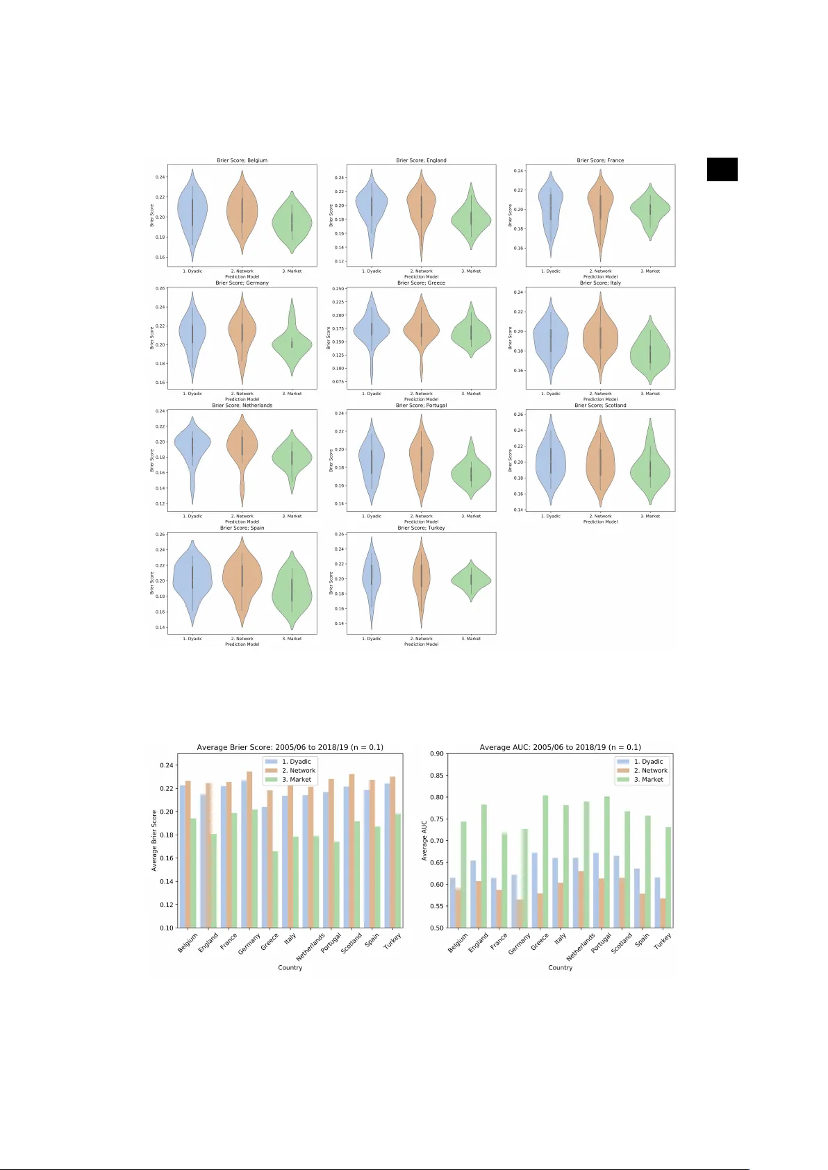
Subject Areas: Comple xity Ke ywor ds: F ootball, Network, P erdition, Centrality A uthor for correspondence: T aha Y asseri e-mail: taha.yasseri@ucd.ie F ootball is becoming more predictab le; Network analysis of 88 thousands matches in 11 major leagues Victor Mar tins Maimone 1 and T aha Y asseri 1 , 2 , 3 , 4 1 Oxf ord Inter net Institute, Univ ersity of Oxford, Oxf ord O X1 3JS, UK 2 Alan T uring Institute, London NW1 2DB , UK 3 School of Sociology , University College Dub lin, Dublin 4, Ireland 4 Gear y Institute f or Public P olicy , Univ ersity College Dublin, Dub lin 4, Ireland In recent years excessive monetization of football and professionalism among the players has been argued to have affected the quality of the match in differ ent ways. On the one hand, playing football has become a high-income profession and the players are highly motivated; on the other hand, stronger teams have higher incomes and therefor e afford better players leading to an even stronger appearance in tournaments that can make the game more imbalanced and hence predictable. T o quantify and document this observation, in this work we take a minimalist network science approach to measur e the predictability of football over 26 years in major European leagues. W e show that over time, the games in major leagues have indeed become more predictable. W e provide further support for this observation by showing that inequality between teams has increased and the home-field advantage has been vanishing ubiquitously . W e do not include any direct analysis on the effects of monetization on football’s predictability or therefor e, lack of excitement, however , we pr opose several hypotheses which could be tested in future analyses. 2 . . 1. Introduction Playing football is, arguably , fun. So is watching it in stadiums or via public media, and to follow the news and events around it. Football is worthy of extensive studies, as it is played by r oughly 250 million players in over 200 countries and dependencies, making it the world’s most popular sport [ 1 ]. Eur opean leagues alone ar e estimated to be worth more than £20 billion [ 2 ]. The sport itself is estimated to be worth almost thirty times as much [ 3 ]. In Figur e S1 the combined revenue for the big 5 European leagues over time are shown. The overall revenues have been steadily increasing over the last two decades [ 4 ]. It has been argued that the surprise element and unpredictability of football is the key to its popularity [ 5 ]. A major question in relation to such a massive entertainment enterprise is if it can retain its attractiveness through surprise element or , due to significant recent monetisations, it is becoming more predictable and hence at the risk of losing popularity? T o address this question, a first step is to establish if the predictability of football has indeed been increasing over time. This is our main aim here; to quantify predictability , we devise a minimalist prediction model and use its performance as a proxy measur e for predictability . There has previously been a fair amount of research in statistical modelling and forecasting in relation to football. The Prediction models are generally either based on detailed statistics of actions in the pitch [ 6 – 9 ] or on a prior ranking system which estimates the relative strengths of the teams [ 10 – 12 ]. Some models have considered team pairs attributes such as the geographical locations [ 7 , 13 , 14 ], and some models have mixed these approaches [ 15 , 16 ]. A rather new approach in predicting performance is based on machine learning and network science [ 17 , 18 ]. Such methods have been used in r elation to sport [ 19 – 21 ] and particularly football [ 22 , 23 ]. Most of the past research in this area however either focuses on inter-team interactions and modelling player behaviour rather than league tournament’s results prediction, or are limited in scope—particularly they rar ely take a historical approach in or der to study the game as an evolving phenomenon [ 24 – 26 ]. This is understandable in light of the fact that most of these methods are data-thirsty and therefor e not easy to use in a historical context where extensive datasets are unavailable for games played in the past. In the present work, we use a network science approach to quantify the predictability of football in a simple and robust way without the need for an extensive dataset and by calculating the measures in 26 years of 11 major Eur opean leagues we examine if predictability of football has changed over time. 2. Results and Discussion The pr edictive model and the method of quantifying its performance are presented in the Materials and Methods section. After having assessed the models’ validity and robustness, here we address if the pr edictability of football has been changing over time. (a) Predictability ov er Time In Figure 1 we see the AUC scores (a measure of the performance of the model) and a smoothed fits to them per league over time, for the last 26 years (and in Figure S13 you see similar trends measured by Brier score). A positive trend in predictability is observed in most of the cases (England, France, Germany , Netherlands, Portugal, Scotland and Spain) and, for the cases of the top leagues (England, Germany , Portugal and Spain), the graphical intuition is corroborated by a comparison between the earlier and later parts of their respective samples using the Student t-test. W e compared the first 10 years with the last 10 years and reported the p-value for the test (under the null hypothesis that the expected values are the same). W e also compared the two distributions under the KS test to check whether they wer e similar (under the null hypothesis that they wer e). Both set of p-values are reported in T able 1 . The remaining leagues display somewhat 3 . . Figure 1. Time T rends In A UC and Gini Coefficient. Blue dots/lines depict A UC and are marked in the primar y (left) y -axis; Orange dots/lines depict the Gini coefficient and are mar k ed in the secondar y (right) y -axis; Both lines are fitted through a lowess model. stable predictability throughout time. All leagues, notwithstanding, tend to converge towards 0.75 AUC. (b) Increasing Inequality In analysing the pr edictability of different leagues, we observe that predictability has been increasing for the richer leagues in Eur ope, whereas the set for which the indicator is deteriorating is composed mainly of peripheral leagues. It seems football as a sport is emulating society in its somewhat “gentrification” process, i.e., the richer leagues are becoming more deterministic because better teams win more often; consequentially , becoming richer; allowing themselves to hire better players (fr om a talent pool that gets internationally br oader each year); becoming even str onger; and, closing the feedback cycle, winning even more matches and tournaments; hence more pr edictability in more professional and expensive leagues. T o illustrate this trend, we use the Gini coefficient, proposed as a measure of inequality of income or wealth [ 27 – 29 ]. W e calculate the Gini coefficient of a given league-season’s distribution of points each team had at the end of the tournament. Figure 1 depicts the values for all the leagues in the database, comparing the evolution of predictability and the evolution of inequality 4 . . T able 1. The p-values from comparing the a verage Network Model A UC , Inequality Coefficient (Gini) and the Elo-System A UC (ELO-AUC) f or the two parts of each countr y’ s sample, under the null hypothesis the e xpected v alues are the same using the Student t-test. We also present the p-values for the distributions under the KS test to check whether they were similar (under the null h ypothesis that they were). Country AUC: KS AUC: t Gini: KS Gini: t ELO_AUC: KS ELO_AUC: t Belgium 0.9985 0.7383 0.2558 0.0752 0.8690 0.4805 England 0.1265 0.0330 0.0126 0.0009 0.0443 0.0133 France 0.1265 0.1437 0.2999 0.3426 0.1265 0.0895 Germany 0.1265 0.0326 0.2999 0.0367 0.5882 0.0787 Greece 0.2558 0.0634 0.5361 0.1190 0.0079 0.0019 Italy 0.2999 0.7370 0.0443 0.0547 0.9992 0.8292 Netherlands 0.8978 0.7371 0.5882 0.9488 0.8978 0.8320 Portugal 0.0079 0.0044 0.0000 0.0000 0.0314 0.0071 Scotland 0.9985 0.9128 0.0314 0.0771 0.5361 0.2864 Spain 0.0443 0.0097 0.0005 0.0001 0.0029 0.0010 T urkey 0.9985 0.6429 0.8690 0.4610 0.2558 0.3108 T able 2. A UC and Gini Correlation by league League Correlation Spain 0.874 England 0.823 Germany 0.805 Scotland 0.723 Portugal 0.694 T urkey 0.686 League Correlation Netherlands 0.676 Italy 0.622 France 0.563 Greece 0.561 Belgium 0.413 between teams for each case. There is a high correlation between predictability in a football league and inequality amongst teams playing in that league, uncovering evidence in favour of the “gentrification of football” argument. The correlation values between these two parameters are r eported in T able 2 . (c) Home Advantage and Predictability As described in the Materials and Methods section, our predictive model also quantifies the home-field advantage. W e calculated the average amount of home-field advantage as measured in the pr ediction models ( µ in Eq. 4.1 ) for each season of English Premier League and plotted it in Figure. 2 . W e see a decrease in home field advantage over time (for the results for other leagues see Figures S2 –S5.) However , one can calculate the home advantage directly from historical data by counting the total number of points that the home and away teams gained in each season. The trends in the share of home teams for different leagues are shown in Figure 2 (For detailed diagrams of each league see Figures S2–S5). It is clear that the home-field advantage is still present, however , it has been decreasing throughout time for all the leagues under study . In explaining this trend, we should consider factors involved in home-field advantage. Pollard counts the following as driving factors for the existence of home-field advantage [ 30 ]: cr owd effects; travel effects; familiarity with the pitch; refer ee bias; territoriality; special tactics; rule factors; psychological factors; and the interaction between two or mor e of such factors. While some of these factors are not changing over time, incr ease in the number of foreign players, diminishing the effects of territoriality and its psychological factors, as well as observing that fewer people ar e going to stadiums, travelling 5 . . Figure 2. The Decrease in Home Field Adv antage. Left: Home field advantage calculated by the two models. Right: The share of home points measured on historical data. The straight lines are linear fits. See the detailed graphs for each league in Figures S8–S11. is becoming easier , teams are camping in different pitches and players are accruing more international experience, can explain the reported trend; stronger (richer) teams are much more likely to win, it matters less where they play . 3. Conclusion Relying on large-scale historical recor ds of 11 major football leagues, we have shown that, throughout time, football is dramatically changing; the sport is becoming more predictable; teams are becoming increasingly unequal; the home-field advantage is steadily and consistently decreasing for all the leagues in the sample. The prediction model in this work is designed to be self-contained, i.e., to solely consider the past results as supporting data to understand future events. Despite the str ength in terms of time consistency , it does not rely on the myriad of data that are available nowadays, which is being extensively used by cutting edge data science projects [ 31 ] and, obviously , the betting houses. In this sense, this work is limited by the amount of data and the sophistication of the models it considers, however , this is by design and in order to focus on the nature of the system under study rather than the predictive models. Furthermore, this work is also limited by the sample size; Football has been played in over 200 countries, out of which only 5.5% were included in our sample. Although the main reasons for that ar e of practical matters, given the hardship in obtaining r eliable and time-consistent data, the events become very sparse for most of the leagues going back in time. Future work should, as speculated in this work, try and assess: the role money is playing in removing the surprise element of the sport; expanding the sample barriers to include continent level tournaments (such as The UEF A Champions League) and to beyond the Eur opean continent; and ultimately , but not exhaustively , should test the money impact over predictability on differ ent sports and leagues that – theoretically – should not be affected by it, namely leagues and sports that impose salary caps over their teams, such as the United States of America’s Professional Basketball League (the NBA). 4. Data and Methods 6 . . T able 3. Database – Matches per league Country T otal Matches Belgium 6620 England 10044 France 9510 Germany 7956 Greece 6470 Italy 9066 Country T otal Matches Netherlands 7956 Portugal 7122 Scotland 5412 Spain 10044 T urkey 7616 (a) Data In this study , each datapoint depicts a football match and, as such, contains: the date in which the match took place, which determines the season for which the match was valid; the league; the home team; the away team; the final score (as in, the final amount of goals scored by each team); and the pay-offs at Bet 365 betting house. The database encompasses eleven differ ent European countries and their top division leagues (Belgium, England, France, Germany , Greece, Italy , Netherlands, Portugal, Scotland, Spain and T urkey), ranging from the 1993-1994 to the 2018-2019 seasons (some leagues only have data starting in the 1994-1995 and 1995-1996 seasons). The data was extracted from https://www. football- data.co.uk/ . Considering all leagues and seasons, the final database encompasses 87,816 matches (See T able 3 ). These 87,816 matches had a total of 236,323 goals scored, an average of 2.7 goals per match. (b) Modelling predictability T o measure the predictability of football based on a minimum amount of available data, we need to build a simple prediction model. For the sake of simplicity and interpretability of our model, we limit our analysis to the matches that have a winner and we eliminate the ties fr om the entirety of this study . T o include the ties an additional parameter would be needed which makes the comparison between differ ent years (different model tuning) irrelevant. Figure S6 shows the percentage of matches ending in a tie is either constant or slightly diminishing throughout time for all but two countries. Our prediction task, therefore, is simplified to predicting a home win versus an away win that refer to the events of the host, or the guest team wins the match respectively . T o predict the results of a given match, we consider the performance of each of the two competing teams in their past N matches preceding that given match. T o be able to compare leagues with different numbers of teams and matches, we normalize this by the total number of matches played in each season T , and define the model training window as n = N/T . For each team, we calculate its accumulated Dyadic Score as the fraction of points the team has earned during the window n to the maximum number of points that the team could win during that window . Using this score as a proxy of the team’s strength, we can calculate the difference between the strengths of the two teams prior to their match and train a predictive model which considers this differ ence as the input. However , this might be too much of a naive predictive model, given that the two teams have most likely played against different sets of teams and the points that they collected can mean differ ent levels of strength depending on the strength of the teams that they collected the points against. W e propose a network-based model in or der to improve the naive dyadic model and account for this scenario. (i) Network Model T o overcome the above-mentioned limitation and come up with a scoring system that is less sensitive to the set of teams that each team has played against, we build a directed network of 7 . . Figure 3. The network diagram of the 2018-2019 English Premier League after 240 matches hav e been play ed for n = 0 . 5 (calculating centrality scores based on the last 190 matches). all the matches within the training window , in which the edges point from the loser to the winner , weighted by the number of points the winner earned. In the next step, we calculate the network eigenvector centrality score for all the teams. The recursive definition of eigenvector centrality , that is that the score of each node depends on the score of its neighbours that send a link to it, perfectly solves the pr oblem of the dyadic scoring system mentioned above [ 17 , 32 , 33 ]. An example of such network and calculated scores ar e presented in Figure 3 . W e can calculate the score dif ference between the two competing teams for any match after the N th match. W e will have ( T − N ) matches with their respective outcomes and score differences , for both models. W e then fit a logistic regression model of the outcome (as a categorical y variable) over the score differ ences according to Eq. 4.1 . W ithout loss of generality , we always calculate the point score differ ence as x = home team score − a wa y team score and assume y = 1 / 0 if the home/away team wins. y = F ( x | µ, s ) = 1 1 + exp( − x − µ s ) , (4.1) where µ and s are model parameters than can be obtained by or dinary least squares methods. Finally , the logistic regression model will provide the probabilistic assessment of each scor e system (Dyadic and Network) for each match, allowing us to understand how correctly the outcomes are being split as a function of the pre-match score difference. See Figure 4 for an example. (ii) Quantifying home adv antage In Figure 4 we see that the fitted Sigmoid is not symmetric and a shift in the probable outcome (i.e., when P rob ( y = 1) ≥ 0 . 50 ) happens at an x value smaller than zero, meaning even for some negative values of x , which r epresents cases where the visiting team’s scor e is greater than the home team’s scor e, we still observe a higher chance for a home team victory . This is not surprising 8 . . Figure 4. Logistic regression model example for the England Premier League 2018-2019 for the two models and the benchmark model. considering the existence of the notion of Home Field Advantage : a significant and structural differ ence in outcome contingent on the locality in which a sports match is played —favouring the team established in such locality , has been exhaustively uncover ed between dif ferent team sports and between dif ferent countries both for men’s and women’s competitions [ 34 ]. Home field advantage was first formalised for North-American sports [ 35 ] and then documented specifically for association football [ 36 ]. (iii) Benchmark Model W e benchmark our models against the implicit prediction model provided by the betting market payoffs ( Bet 365 ). When betting houses allow players to bet on an event outcome, they are essentially pr oviding an implicit probabilistic assessment of that event thr ough the payof f values. W e calculate the probabilities of differ ent outcomes as the following:    P rob ( H omeW in ) = 1 h 1 h + 1 a P rob ( Aw ayW in ) = 1 a 1 h + 1 a , (4.2) where h is monetary units for a home team win, a units for an away team win. The experienced gambler knows that in the r eal world, on any given betting house’s game, the sum of the outcomes’ probabilities never does equal to 1, as the game proposed by the betting houses is not strictly fair . However , we believe this set of probabilities give us a good estimate of the state of the art predictive models in the market. In Figure 4 the data and corresponding fits to all the 3 models are pr ovided. (iv) The Elo Ranking System The problem of ranking teams/players within a tournament based not only on their victories and defeats but also on how hard those matches were expected to be beforehand is rather explored throughout the literature. Arpad Elo [ 37 ] proposed what became the first ranking system to explicitly consider such caveat, as follows: New players/teams start with a numeric rating ( R i ) of 1,500. Prior to each match we calculate the expected result for each team ( E i ), which is a quasi-normal function of the differ ence between the teams’ current rankings ( R i and R j ): E i = 1 1 + 10 R j − R i 400 (4.3) After the match, we update the rankings given the dif ference between the expected outcome and the actual one: 9 . . R 0 i = R i + K ( S i − E i ) , (4.4) Where S i is the binary outcome of the match between teams/players i and j and E i is the expected outcome for player/team i , as determined by Equation 4.3 . Note a K-Factor is proposed, which serves as a weight on how much the result will impact the new rating for the teams/players. Elo himself pr oposed two values of K when ranking chess players, depending on the play er ’s classification (namely 16 for a chess master and 32 for lower -ranked players). Despite the rating itself being composed of a prediction, we applied the same dynamics under which we analysed the prior models: we calculated the rating for both teams prior to each match and used the difference between ratings (home minus away) to fit a logistic curve (with 1 for a home win, 0 for an away win). (c) Model P erf or mance Assessing the performance of a probabilistic model is both challenging and controversial in the literature, as the different measures present strengths and weaknesses. Notwithstanding, the majority of research done in the area applies (at least one of) two methods, namely: a loss function; and/or a binary accuracy measure. W e analyse our models within both approaches and also benchmark the proposed network model against an established ranking model, known as the Elo Ranking Model (see below). (i) Loss Function: The Brier Score Proposed in [ 38 ], the Brier score is a loss function that measures the accuracy of probabilistic predictions. It applies to tasks in which predictions must assign probabilities to a set of mutually exclusive discrete outcomes. The set of possible outcomes can be either binary or categorical in natur e, and the probabilities assigned to this set of outcomes must sum to one (where each individual probability is in the range of 0 to 1). Suppose that on each of t occasions an event can occur in only one of r possible classes or categories and on one such occasion, i , the for ecast probabilities are f i 1 , f i 2 , ..., f ir , that the event will occur in classes 1 , 2 , ..., r , respectively . The r classes are chosen to be mutually exclusive and exhaustive so that P r j =1 f ij = 1 , i = 1 , 2 , 3 , ..., t . Hence, the Brier score is defined as: P = 1 t r X j =1 t X i =1 ( f ij − E ij ) 2 (4.5) where E ij takes the value 1 or 0 according to whether the event occurred in class j or not. In our case, we have: r = 2 classes, i.e., either the home team won or not; and (1 − n ) T matches to be predicted, transforming Equation 4.5 into: P = 1 (1 − n ) T 2 X j =1 (1 − n ) T X i =1 ( f ij − E ij ) 2 , (4.6) W e see, from Equation 4.6 , how the Brier Score is an averaged measure over all the predicted matches, i.e., each league-season combination will have its own single Brier Score. The lower the Brier scor e, the better (as in the mor e assertive and/or correct) our prediction model. In Figur e S7 the distributions of Brier scores for dif ferent models are shown. (ii) Accuracy: Receiv er Operating Characteristic (ROC Curve) A receiver operating characteristic curve , or ROC curve, is a graphical plot that illustrates the diagnostic ability of a binary classifier system as its discrimination threshold is varied, which allows us to generally assess a prediction method’s performance for different thresholds. When using normalised units, the area under the ROC curve (often referred to as simply the AUC) is 10 . . Figure 5. Area Under the Cur v e (AUC) distributions per country for the benchmark and prediction models (f or n = 0 . 5 ). equal to the probability that a classifier will rank a randomly chosen positive instance higher than a randomly chosen negative one [ 39 ]. The machine learning community has historically used this measure for model comparison [ 40 ], though the practice has been questioned given AUC estimates are quite noisy and suffer from other problems [ 41 – 43 ]. Nonetheless, the coherence of AUC as a measure of aggregated classification performance has been vindicated, in terms of a uniform rate distribution [ 44 ], and AUC has been linked to several other performance metrics, including the above mentioned Brier score [ 45 ]. In Figur e S8 the distributions of Brier scores for differ ent models are shown. T o compare our two models with the benchmark model, we calculate a loss function in the form of the Brier score for all the (1 − n ) T matches in different leagues and years from 2005 to 2018 and n = 0 . 5 . The distributions of scores ar e reported in Figure S1 and the average scores are shown in Figure 6 (a) (Note that the smaller the Brier score, the better fit of the model). Progr essing on the loss function to actual prediction accuracy , for each match, we considered a home team win prediction whether P rob ( H omeW in ) ≥ π and an away team win prediction otherwise. W e applied this prediction rule for all three models (Dyadic, Network and the Betting Houses Market benchmark) and compared the predictions to the outcomes, calculating how many predictions matched the outcome. Note that the betting market prediction data ar e only available for more recent years (13 years) therefore our comparison is limited to those years. W e change the threshold of π and calculate the average Area Under Curve (AUC) score of Receiver 11 . . Figure 6. Accuracy of the models measured through a)average Br ier Score and b) area Under the Cur v e (A UC), per league. Operating Characteristic (ROC Curve) for each league, shown in Figure 6 (b). The complete set of distributions for the accuracy indicators is depicted in Figures S1 and S2. By increasing n , naturally the accuracy of predictions increases. For the rest of the paper , however , we focus on n = 0 . 5 . The comparisons for different values of n is presented in Figures S9-S12. Even though our model underperforms the market on average, t-tests for the differ ence between the Brier score and AUC distributions of our models and the betting houses market are statistically indistinguishable at the 2% significance level for the majority of year-leagues (See T ables S1 and S2 for details). One should note that the goal here is not to develop a better prediction model than the one provided by the betting houses market but to obtain a comparable, consistent and simple-to-calculate model. Market models evolve throughout time, which would bias the assessment of a single prediction tool throughout the years. In that capacity , we are looking for models that provide the time-robust tool we need to assess whether football is becoming more pr edictable over the years. T o compare the network model with the Elo-based model, we calculated the AUC for the Elo- based model for each country-season combination and plotted it against the Network model. The results are surprisingly similar , but the Network model outperforms an Elo-based model (with a K-Factor of 32), as we can see from Figure S13. Specifically , the Network model scores a higher AUC value in roughly 61% of cases (170 of 280). Nevertheless, the results for the trends in pr edictability holds for the Elo-based model too. However , as said above, what matters the most is the ease in training of the model and the consistency of its predictions rather than slight advantages in performance. Data A vailability: The datasets used and analysed during the current study are available in the Supplementary file 2 dataset.zip and at https://doi.org/10.5061/dryad.8931zcrrs . Author Contribution: VM collected and analysed the data. TY designed and supervised the resear ch. Both authors wrote the article. Funding: TY was partially supported by the Alan T uring Institute under the EPSRC grant no. EP/N510129/1. Acknowledgement The authors thank Luca Pappalardo for valuable discussions. 12 . . Ref erences 1. Giulianotti R, Rollin J, W eil E, Joy B, Alegi P . 2017 Football. Encyclopedia Britannica. . 2. W ilson B. 2018 European football is worth a recor d £22bn, says Deloitte. . 3. Ingle S, Glendenning B. 2003 Baseball or Football: which sport gets the higher attendance?. . 4. Ajadi T , Ambler T , Dhillon S, Hanson C, Udwadia Z, W ray I. 2021 Annual Review of Football Finance 2021. Report Deloitte. 5. Choi D, Hui SK. 2014 The r ole of surprise: Understanding overreaction and underreaction to unanticipated events using in-play soccer betting market. Journal of Economic Behavior & Organization 107 , 614–629. 6. Maher MJ. 1982 Modelling association football scores. Statistica Neerlandica 36 , 109–118. 7. Rue H, Salvesen O. 2000 Prediction and retr ospective analysis of soccer matches in a league. Journal of the Royal Statistical Society: Series D (The Statistician) 49 , 399–418. 8. Dixon MJ, Coles SG. 1997 Modelling association football scores and inefficiencies in the football betting market. Journal of the Royal Statistical Society: Series C (Applied Statistics) 46 , 265–280. 9. Crowder M, Dixon M, Ledford A, Robinson M. 2002 Dynamic modelling and pr ediction of English Football League matches for betting. Journal of the Royal Statistical Society: Series D (The Statistician) 51 , 157–168. 10. Hvattum LM, Arntzen H. 2010 Using ELO ratings for match result prediction in association football. International Journal of forecasting 26 , 460–470. 11. Buchdahl J. 2003 Fixed odds sports betting: Statistical forecasting and risk management . Summersdale Publishers L TD-ROW . 12. Constantinou AC, Fenton NE, Neil M. 2012 pi-football: A Bayesian network model for forecasting Association Football match outcomes. Knowledge-Based Systems 36 , 322–339. 13. Goddard J, Asimakopoulos I. 2004 Forecasting football r esults and the ef ficiency of fixed-odds betting. Journal of Forecasting 23 , 51–66. 14. Kuypers T . 2000 Information and efficiency: an empirical study of a fixed odds betting market. Applied Economics 32 , 1353–1363. 15. Goddard J. 2005 Regression models for forecasting goals and match results in association football. International Journal of forecasting 21 , 331–340. 16. Baboota R, Kaur H. 2019 Predictive analysis and modelling football r esults using machine learning approach for English Pr emier League. International Journal of Forecasting 35 , 741–755. 17. Fraiberger SP , Sinatra R, Resch M, Riedl C, Barabási AL. 2018 Quantifying reputation and success in art. Science 362 , 825–829. 18. W illiams OE, Lacasa L, Latora V . 2019 Quantifying and predicting success in show business. Nature communications 10 , 2256. 19. Cintia P , Coscia M, Pappalardo L. 2016 The Haka network: evaluating rugby team performance with dynamic graph analysis. In Proceedings of the 2016 IEEE/ACM International Conference on Advances in Social Networks Analysis and Mining pp. 1095–1102. IEEE Press. 20. Radicchi F . 2011 Who is the best player ever? A complex network analysis of the history of professional tennis. PloS one 6 , e17249. 21. Y ucesoy B, Barabási AL. 2016 Untangling performance from success. EPJ Data Science 5 , 17. 22. Rossi A, Pappalar do L, Cintia P , Iaia FM, Fernàndez J, Medina D. 2018 Ef fective injury forecasting in soccer with GPS training data and machine learning. PloS one 13 , e0201264. 23. Pappalardo L, Cintia P , Ferragina P , Pedreschi D, Giannotti F . 2018 PlayeRank: Multi-dimensional and role-aware rating of soccer player performance. arXiv preprint arXiv:1802.04987 . 24. Cintia P , Rinzivillo S, Pappalardo L. 2015 A network-based approach to evaluate the performance of football teams. In Machine learning and data mining for sports analytics workshop, Porto, Portugal . 25. Lazova V , Basnarkov L. 2015 PageRank approach to ranking national football teams. arXiv preprint arXiv:1503.01331 . 26. Milanlouei S. 2017 Fall In Love W ith Network Science At First Sight!. . 27. Gini C. 1912 V ariabilità e mutabilità. Reprinted in Memorie di metodologica statistica (Ed. Pizetti E, Salvemini, T). Rome: Libreria Eredi V irgilio V eschi . 28. Gini C. 1921 Measurement of inequality of incomes. The Economic Journal 31 , 124–126. 29. Gini C. 1936 On the measure of concentration with special reference to income and statistics. Colorado College Publication, General Series 208 , 73–79. 13 . . 30. Pollard R. 2008 Home advantage in football: A current review of an unsolved puzzle. The open sports sciences journal 1 . 31. Pappalardo L, Cintia P . 2017 Quantifying the relation between performance and success in soccer . Advances in Complex Systems p. 1750014. 32. Newman M. 2018 Networks . Oxford university press. 33. Bonacich P . 1987 Power and centrality: A family of measures. American journal of sociology 92 , 1170–1182. 34. Pollard R, Prieto J, Gómez MÁ. 2017 Global differences in home advantage by country , sport and sex. International Journal of Performance Analysis in Sport 17 , 586–599. 35. Schwartz B, Barsky SF . 1977 The home advantage. Social forces 55 , 641–661. 36. Pollard R. 1986 Home advantage in soccer: A retrospective analysis. Journal of sports sciences 4 , 237–248. 37. Elo AE. 1978 The rating of chessplayers, past and present . Arco Pub. 38. Brier GW . 1950 V erification of forecasts expressed in terms of probability . Monthey Weather Review 78 , 1–3. 39. Fawcett T . 2006 An introduction to ROC analysis. Pattern recognition letters 27 , 861–874. 40. Hanley JA, McNeil BJ. 1983 A method of comparing the areas under receiver operating characteristic curves derived from the same cases.. Radiology 148 , 839–843. 41. Hanczar B, Hua J, Sima C, W einstein J, Bittner M, Dougherty ER. 2010 Small-sample precision of ROC-related estimates. Bioinformatics 26 , 822–830. 42. Lobo JM, Jiménez-V alverde A, Real R. 2008 AUC: a misleading measure of the performance of predictive distribution models. Global ecology and Biogeography 17 , 145–151. 43. Hand DJ. 2009 Measuring classifier performance: a coherent alternative to the area under the ROC curve. Machine learning 77 , 103–123. 44. Ferri C, Hernández-Orallo J, Flach P A. 2011 A coherent interpretation of AUC as a measure of aggregated classification performance. In Proceedings of the 28th International Conference on Machine Learning (ICML-11) pp. 657–664. 45. Hernández-Orallo J, Flach P , Ferri C. 2012 A unified view of performance metrics: translating threshold choice into expected classification loss. Journal of Machine Learning Research 13 , 2813– 2869. 14 . . Suppor ting Inf or mation for "F ootball is becoming more predictable; Network analysis of 88 thousands matches in 11 major leagues" Victor Mar tins Maimone and T aha Y asseri T able S1. The t-T est values comparing the Brier scores for the prediction models and the betting house benchmark for n = 0 . 5 . Country Model t-stat p-value . . . . . . . . . . . . . . .. . . . . . . . . . . . . . . . . . . . . . . . . . . . .. . . . . . . . . . . . . . . . . . . . . . . . . . . . . .. . . . . . . . . . . . . . . . . . . . . . . . . . . . . .. . . . . . . . . . . . . . . . . . . . . . . . . . . . . .. . . . . . . . . . . . . . . . . . . . . . . . . . . . . .. . . . . . . . . . . . . . . . . . . . . . . . . . . . .. . . . . . . . . . . . . . . . . . . . . . . . . . . . . .. Belgium Network 2.679 0.011 England Network 2.801 0.008 France Network 0.549 0.586 Germany Network 2.055 0.048 Greece Network 1.054 0.299 Italy Network 3.422 0.002 Netherlands Network 2.420 0.021 Portugal Network 2.847 0.007 Scotland Network 1.097 0.282 Spain Network 2.382 0.024 T urkey Network 0.459 0.649 Country Model t-stat p-value . . . . . . . . . . . . . . .. . . . . . . . . . . . . . . . . . . . . . . . . . . . .. . . . . . . . . . . . . . . . . . . . . . . . . . . . . .. . . . . . . . . . . . . . . . . . . . . . . . . . . . . .. . . . . . . . . . . . . . . . . . . . . . . . . . . . . .. . . . . . . . . . . . . . . . . . . . . . . . . . . . . .. . . . . . . . . . . . . . . . . . . . . . . . . . . . .. . . . . . . . . . . . . . . . . . . . . . . . . . . . . .. Belgium Dyadic 2.386 0.023 England Dyadic 2.903 0.007 France Dyadic 0.562 0.578 Germany Dyadic 1.894 0.067 Greece Dyadic 0.918 0.365 Italy Dyadic 3.021 0.005 Netherlands Dyadic 2.455 0.019 Portugal Dyadic 2.686 0.011 Scotland Dyadic 1.335 0.192 Spain Dyadic 2.404 0.023 T urkey Dyadic 0.454 0.653 15 . . Figure S1. Reven ue of the biggest European leagues from 1996 to 2021; 2021 and 2022 values are projections. Figure S2. The Decrease in Home Field Advantage: Selected Countries (1/4) 16 . . T able S2. The t-T est values comparing the AUC scores for the prediction models and the betting house benchmark for n = 0 . 5 . Country Model t-stat p-value . . . . . . . . . . . . . . .. . . . . . . . . . . . . . . . . . . . . . . . . . . . .. . . . . . . . . . . . . . . . . . . . . . . . . . . . . .. . . . . . . . . . . . . . . . . . . . . . . . . . . . . .. . . . . . . . . . . . . . . . . . . . . . . . . . . . . .. . . . . . . . . . . . . . . . . . . . . . . . . . . . . .. . . . . . . . . . . . . . . . . . . . . . . . . . . . .. . . . . . . . . . . . . . . . . . . . . . . . . . . . . .. Belgium Network -3.450 0.001 England Network -3.868 0.000 France Network -2.582 0.014 Germany Network -4.576 0.000 Greece Network -1.994 0.054 Italy Network -4.418 0.000 Netherlands Network -3.544 0.001 Portugal Network -4.413 0.000 Scotland Network -1.929 0.062 Spain Network -4.418 0.000 T urkey Network -1.324 0.194 Country Model t-stat p-value . . . . . . . . . . . . . . .. . . . . . . . . . . . . . . . . . . . . . . . . . . . .. . . . . . . . . . . . . . . . . . . . . . . . . . . . . .. . . . . . . . . . . . . . . . . . . . . . . . . . . . . .. . . . . . . . . . . . . . . . . . . . . . . . . . . . . .. . . . . . . . . . . . . . . . . . . . . . . . . . . . . .. . . . . . . . . . . . . . . . . . . . . . . . . . . . .. . . . . . . . . . . . . . . . . . . . . . . . . . . . . .. Belgium Dyadic -3.379 0.002 England Dyadic -3.911 0.000 France Dyadic -2.551 0.015 Germany Dyadic -4.284 0.000 Greece Dyadic -1.852 0.073 Italy Dyadic -4.021 0.000 Netherlands Dyadic -3.679 0.001 Portugal Dyadic -4.389 0.000 Scotland Dyadic -2.049 0.048 Spain Dyadic -4.430 0.000 T urkey Dyadic -1.281 0.208 T able S3. The p-values for the expected amount of ties from the two halves of each country’s sample, under the null hypothesis that the e xpected values are the same. Country T -T est KS-T est . . . . . . . . . . . . . . .. . . . . . . . . . . . . . . . . . . . . . . . . . . . .. . . . . . . . . . . . . . . . . . . . . . . . . . . . . .. . . . . . . . . . . . . . . . . . . . . . . . . . . . . .. . . . . . . . . . . . . . . . . . . . . . . . . . . . . .. . . . . . . . . . . . . . . . . . . . . . . . . . . . . .. . . . . . . . . . . . . . . . . . . . . . . . . . . . .. . . . . . . . . . . . . . . . . . . . . . . . . . . . . .. All Sample 0.061750 0.299920 Belgium 0.455958 0.536098 England 0.119114 0.299920 France 0.436526 0.897806 Germany 0.190617 0.299920 Greece 0.014492 0.099547 Italy 0.016615 0.126488 Netherlands 0.713263 0.897806 Portugal 0.620980 0.868982 Scotland 0.659728 0.998485 Spain 0.000056 0.000500 T urkey 0.023387 0.255775 17 . . Figure S3. The Decrease in Home Field Advantage: Selected Countries (2/4) 18 . . Figure S4. The Decrease in Home Field Advantage: Selected Countries (3/4) 19 . . Figure S5. The Decrease in Home Field Advantage: Selected Countries (4/4) Figure S6. The Percentage of Matches Ending in a Tie . The line shows a non-parametric lowess fitting model 20 . . Figure S7. Br ier score distrib utions per country for the benchmark and prediction models (for n = 0 . 5 ). Figure S8. Av erage Accuracy per Countr y: n = 0 . 10 21 . . Figure S9. Av erage Accuracy per Countr y: n = 0 . 30 Figure S10. Av erage Accuracy per Countr y: n = 0 . 70 Figure S11. Av erage Accuracy per Countr y: n = 0 . 90 22 . . Figure S12. Time T rends In The Brier Score per Countr y . The two lines show a linear reg ression fit and a non-parametric lowess fitting model. 23 . . Figure S13. AUC Comparison between Network Model (Blue) and Elo-Based System (Magenta).