Improved approximation and visualization of the correlation matrix

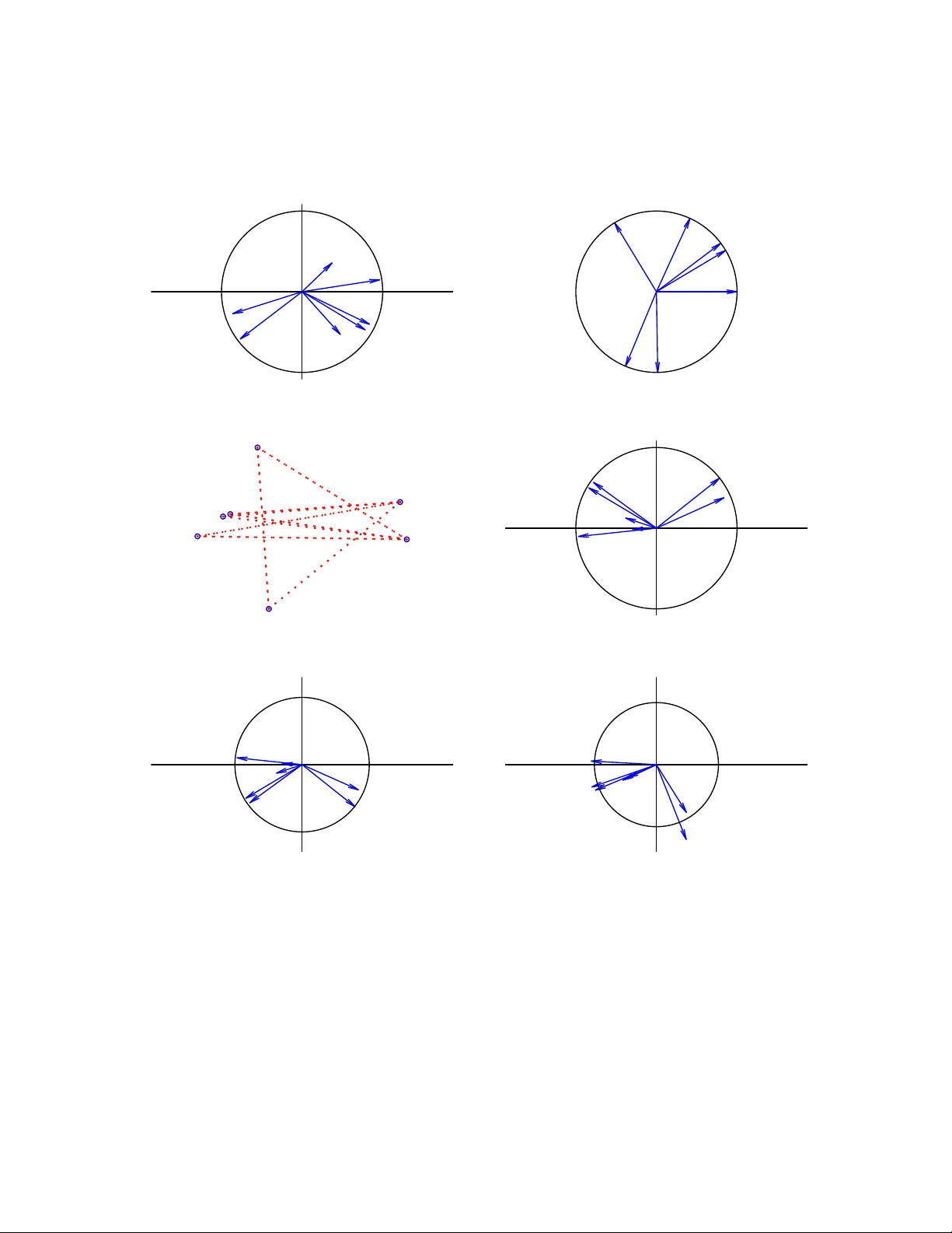
Impro v ed appro ximation and visualization of the correlation matrix Jan Graﬀelman Departmen t of Statistics and Op erations Researc h, Univ ersitat P olit ` ecnica de Catalun y a Departmen t of Biostatistics, Univ ersit y of W ashington Jan de Leeu w Departmen t of Statistics, Univ ersit y of California Los Angeles No v em b er 24, 2022 Abstract The graphical represen tation of the correlation matrix b y means of diﬀerent mul- tiv ariate statistical metho ds is review ed, a comparison of the diﬀeren t pro cedures is presen ted with the use of an example data set, and an impro ved represen tation with b etter ﬁt is proposed. Principal component analysis is widely used for making pic- tures of correlation structure, though as sho wn a w eighted alternating least squares approac h that av oids the ﬁtting of the diagonal of the correlation matrix outperforms b oth principal comp onent analysis and principal factor analysis in appro ximating a correlation matrix. W eighted alternating least squares is a v ery strong comp etitor for principal component analysis, in particular if the correlation matrix is the focus of the study , b ecause it improv es the represen tation of the correlation matrix, often at the exp ense of only a minor p ercen tage of explained v ariance for the original data matrix, if the latter is mapp ed onto the correlation biplot b y regression. In this article, w e prop ose to com bine weigh ted alternating least squares with an additive adjustmen t of the correlation matrix, and this is seen to lead to further impro ved approximation of the correlation matrix. Keywor ds: w eigh ted alternating least squares; biplot; correlogram; m ultidimensional scal- ing; principal comp onen t analysis; principal factor analysis. 1 1 In tro duction The correlation matrix is of fundamental interest in many scien tiﬁc studies that in v olv e m ultiple v ariables, and the visualization of the correlation co eﬃcien t and the correlation matrix has b een the focus of sev eral studies. Hills (1969) prop osed m ultidimensional scaling (MDS), using distances to appro ximate correlations. Ro dgers and Nicewander (1988) re- view m ultiple form ulas for the correlation coeﬃent, showing visualizations that use slop es, angles and ellipses. Murdo c h (1996) prop osed to visualize correlations using a table of elliptical glyphs. F riendly (2002) proposed c orr gr ams that use color and shading of tabu- lar displa ys to represen t the en tries of a correlation matrix. T rosset (2005) dev elop ed the c orr elo gr am , whic h capitalizes on approximation of correlations b y cosines. Obviously , a correlation matrix can be visualized in m ultiple w ays, using diﬀerent geometric principles. In the statistical environmen t R (R Core T eam 2022), visualizations b y means of vector diagrams or biplots can be obtained using the R pack ages FactoMineR (L ˆ e et al. 2008) and factoextra (Kassambara & Mundt 2020, Kassam bara 2017); corrgrams can b e made with the R pac k ages corrgram (W righ t 2021) and corrplot (W ei & Simko 2021). The R pac k ages FactoMineR and factoextra hav e greatly p opularized the visualization of the correlation matrix b y means of a principal comp onen t analysis (PCA). Figure 1 sho ws tw o p opular pictures of the correlation matrix of the m yocardial infarction or Heart attack data (Sap orta 1990), a colored tabular display or corrgram (Fig. 1A) and correlation circle (i.e., a correlation biplot, Fig. 1B) obtained b y PCA. −1 −0.8 −0.6 −0.4 −0.2 0 0.2 0.4 0.6 0.8 1 CI SI VP Pulse logPR DBP P A CI SI VP Pulse logPR DBP P A A: CI SI VP Pulse logPR DBP P A −1.0 −0.5 0.0 0.5 1.0 −1.0 −0.5 0.0 0.5 1.0 Dim1 (56%) Dim2 (17.6%) B: V ariables − PCA Figure 1: Displa ys of the correlation matrix of the Heart attac k data obtained in R b y using the corrplot , FactoMineR and factoextra pac k ages. A: Colored tabular display or corrgram. B: Correlation circle or correlation biplot. See Section 2 for the abbreviations of the v ariable names. Both plots reveal tw o groups of p ositiv ely correlated v ariables (( CI, SI ) and ( Pulse, DBP, P A, VP, lo gPR )) with negativ e correlations b et ween the groups. In this article we 2 fo cus on the visualization of correlations b y means of v ector and scatter diagrams, refrain- ing from coloured tabular represen tations as in Figure 1A. Despite the p opularit y of the correlation circle, from a statistical point of view, PCA giv es a sub optimal approximation of the correlation matrix. The main p oin t of this article is to emphasize and illustrate the impro v ements oﬀered by other metho ds and to stimulate their use ov er just using standard PCA for represen ting correlations. Also, as argued in the Discussion section, the correlation matrix requires go odness-of-ﬁt measures that are diﬀerent from ones sho wn in Figure 1B. 2 Materials and metho ds In this section w e brieﬂy summarize metho ds for the visualization of the correlation matrix using a well-kno wn m ultiv ariate data set, the Heart attack data (Sap orta 1990, pp. 452- 454). The original data consists of 101 observ ations of patients who suﬀered a heart attac k, and for whic h sev en v ariables are registered: the Pulse , the cardiac index ( CI ), the systolic index ( SI ), the diastolic blo od pressure ( DBP ), the pulmonary artery pressure ( P A ), the v en tricular pressure ( VP ) and the pulmonary resistance ( lo gPR ). Pulmonary resistance w as log-transformed in order to linearize its relationship with the other v ariables. W e successiv ely address the representation of correlations by principal comp onent analysis (PCA), the correlogram (CRG), multidimensional scaling (MDS), principal factor analysis (PF A) and weigh ted alternating least squares (W ALS). An additiv e adjustment to the correlation matrix is prop osed to impro ve its visualization b y PCA and W ALS. 2.1 Principal comp onen t analysis Principal comp onent analysis is probably the most widely used metho d to display corre- lation structure by means of a v ector diagram as given in Figure 1B. A correlation-based PCA can b e performed b y the singular v alue decomposition of the standardized data matrix ( X s , scaled b y 1 / √ n ) 1 √ n X s = UD s V 0 , (1) where the left singular vectors are identical to the standardized principal components, and the righ t singular v ectors are eigenv ectors of the sample correlation matrix R since R = 1 n X s 0 X s = VD 2 s V 0 = VD λ V 0 , (2) where the eigen v alues of the correlation matrix are the squares of the singular v alues. The v ectors (arrows) in the correlation circle are given by G = VD s , and represent the en tries of the eigenv ectors scaled b y the singular v alues. A w ell-kno wn prop ert y of this v ector diagram is that cosines of angles θ ij b et ween vectors approximate correlations, as from GG 0 = R it follows that cos ( θ ij ) = g i 0 g j k g i kk g j k ≈ r ij , (3) 3 where g i is the i th row of G . This equation holds true exactly in the full space when using all eigen v ectors, but only appro ximately so if a subset of the ﬁrst few (typically tw o) is used. Besides using cosines, PCA allo ws the approximation of the correlations by using scalar pro ducts b et ween v ectors, suc h that a biplot (Gabriel 1971) of the correlation matrix is obtained. In biplots it is common practice to use scalar products to appro ximate the en tries of a data matrix of in terest, such as a correlation matrix; the entries of the matrix are approximated by the length of the pro jection of one vector onto another, m ultiplied by the length of the v ector pro jected up on. In the case of a correlation matrix, we ha v e, using Eq. (2), r ij ≈ g i 0 g j = cos ( θ ij ) k g i kk g j k = k p i kk g j k , (4) where p i is the pro jection of g i on to g j . Biplots ha v e b een dev elop ed for all classical m ultiv ariate metho ds, and sev eral textbo oks describ e biplot theory and pro vide many ex- amples (Gow er & Hand 1996, Y an & Kang 2003, Greenacre 2010, Gow er et al. 2011). A go odness-of-ﬁt measure, based on least-squares, of the correlation matrix is giv en by tr( ˆ R 0 ˆ R ) tr( R 0 R ) = λ 2 1 + λ 2 2 P p i =1 λ 2 i , (5) where ˆ R is the rank t w o appro ximation obtained from Eq. (2) b y using t wo eigen v ectors only . W e note that this measure is based on the squar es of the eigen v alues, as detailed in the seminal paper by Gabriel (1971), whereas the eigenv alues themselv es are used to calculate the go o dness-of-ﬁt of the cen tered data matrix (See Section 3). 2.2 The correlogram The correlogram, prop osed b y T rosset (2005), explicitly optimizes the appro ximation of correlations in a tw o or three dimensional subspace by cosines, by minimizing the loss function σ ( θ ) = k R − C ( θ ) k 2 with C ( θ ) j k = cos ( θ j − θ k ) , (6) where θ = (0 , θ 2 , . . . , θ p ) is a v ector of angles with resp ect to the x axis, one for eac h v ariable, the ﬁrst v ariable b eing represented by the x axis itself. Equation (6) can b e minimized n umerically , using R’s function nlminb of the standard R pack age stats (R Core T eam 2022). In a correlogram, v ector length is not used in the in terpretation, and all v ariables are therefore represented b y vectors that emanate from the origin, and that ha v e unit length, falling all on a unit circle (see Figure 2B). A linearized v ersion of the correlogram w as prop osed b y Graﬀelman (2013). 2.3 Multidimensional scaling Hills (1969) prop osed to represent correlations b y distances using MDS, and suggested to transform correlations to distances by using the transformation d ij = 2(1 − r ij ), after whic h they are used as input for classical metric m ultidimensional scaling (Mardia et al. 4 1979, Chapter 14), also known as principal co ordinate analysis (PCO; Gow er (1966)). As a historical note, in order to repro duces Hills’ result, one actually needs to use the transformation d ij = p 2(1 − r ij ), implying Hills’ article referred to the squar e d distances. Imp ortan tly , with this transformation the relationship b et w een correlation and distance is ultimately non-linear. Using this distance, tigh tly p ositively correlated v ariables will b e close ( d ij ≈ 0), and tigh tly negativ ely correlated v ariables will b e remote ( d ij ≈ 2), whereas uncorrelated v ariables will app ear at intermediate distance ( d ij ≈ √ 2). Ob viously , the diagonal of ones of the correlation matrix will alw a ys b e perfectly ﬁtted with this approac h. In MDS, go o dness-of-ﬁt is usually assessed by lo oking at the eigen v alues. Ho w ever, in this case the eigenv alues will b e indicativ e of the go o dness-of-ﬁt of the double-centered correlation matrix, not of the original correlation matrix. In order to assess go o dness-of- ﬁt in terms of the ro ot mean squared error ( RMSE ), as we will do for other methods, w e will use the distances ﬁtted b y MDS (in t wo dimensions), and bac ktransform these to obtained ﬁtted correlations in order to calculate the RMSE . A classical metric MDS of correlations transformed to distances by Hills’ transformation is equiv alen t to the spectral decomp osition of the double-c enter e d correlation matrix, which can b e obtained from the ordinary correlation matrix by cen tering columns and rows with a centering matrix H = I − (1 /p ) 11 0 . F or the double-cen tered correlation matrix R dc , w e ha ve that R dc = HRH = (1 /n ) HX s 0 X s H = Z 0 Z , (7) with Z = (1 / √ n ) X s H . It follows that R dc is p ositiv e semideﬁnite, with rank no larger than p − 1, and consequen tly , a conﬁguration of points whose in terp oin t distances exactly represen t the correlation matrix in at most p − 1 dimensions can alw ays b e found (Mardia et al. 1979, Section 14.2). 2.4 Principal factor analysis The classical orthogonal factor mo del for a p -v ariate random v ector x , is giv en by x = Lf + e , where L is the matrix of p × m factor loadings, f the v ector with m latent factors, and e a v ector of errors. This model can be estimated in v arious wa ys. Currently , factor mo dels are mostly ﬁtted using maxim um likelihoo d estimation, which also enables the comparison of diﬀeren t factor mo dels b y likelihoo d ratio tests. PF A is an older iterative algoritm for estimating the orthogal factor mo del (Johnson & Wichern 2002, Harman 1976). It is based on the iterated sp ectral decomp osition of the reduced correlation matrix, which is obtained b y subtracting the sp eciﬁcities from the diagonal of the correlation matrix. A classical factor loading plot is in fact a biplot of the correlation matrix, since the factor mo del implicitly decomp oses the correlation matrix as R = LL 0 + Ψ , (8) where Ψ is the diagonal matrix of sp eciﬁcities (v ariances not accounted for b y the common factors). A lo w-rank appro ximation to the correlation matrix, sa y of rank t wo, is obtained by ˆ R = LL 0 after estimating the t wo-factor mo del. This appro ximation is kno wn to b e b etter than the appro ximation oﬀered by PCA, for it a v oids the ﬁtting of diagonal of the co v ariance or correlation matrix (Satorra & Neudec ker 1998). 5 2.5 W eigh ted alternating least squares In general, a lo w-rank approximation for a rectangular matrix X can b e found by weigh ted alternating least squares, b y minimizing the loss function σ ( A , B ) = n X i =1 p X j =1 w ij ( x ij − a i 0 b j ) 2 , (9) where a i is the i th row of A , b j the j th row of B , W a matrix of w eights and where we seek the factorization X = AB 0 . The unw eighted case ( w ij = 1) is solved b y the singular v alue decomp osition (Eck art & Y oung 1936). Keller (1962) also addressed the un weigh ted case, and explicitly considered the symmetric case. Bailey & Go w er (1990) considered the symmetric case with diﬀerential weigh ting of the diagonal. A general-purp ose algorithm for the w eighted case based on iterated w eighted regressions (”criss cross regressions”) was prop osed b y Gabriel and Zamir (1979); Gabriel (1978) also presented an application in the context of the approximation of a correlation matrix, where w e hav e that X = R . Pietersz and Groenen (2004) present a ma jorization algorithm for minimizing Eq. (9) for the correlation matrix. The ﬁt of the diagonal of the correlation matrix can b e av oided b y using a weigh t matrix W = J − I , where J is a p × p matrix of ones, and I a p × p iden tit y matrix. This w eighting gives weigh t 1 to all oﬀ-diagonal correlations and eﬀectiv ely turns oﬀ its diagonal by giv en it zero w eight. An eﬃcient algorithm and R co de for using W ALS with a symmetric matrix has b een dev elop ed by De Leeuw (2006). The W ALS approac h can outp erform PF A, for not being sub ject to the restrictions of the factor mo del. Comm unalities in factor analysis cannot exceed 1, whic h implies that the rows of the matrix of loadings L are v ectors that are constrained to b e inside, or in the limit, on th e unit circle. In practice, PF A and W ALS give the same RMSE if all v ariable v ectors in PF A fall inside the unit circle, but W ALS ac hiev es a lo w er RMSE whenev er a v ariable v ector reac hes the unit circle in PF A. This t ypically happ ens when a v ariable, in terms of the factor mo del, has a communalit y of one, or equiv alently , zero sp eciﬁty , a condition kno wn as a Heywo o d c ase in maximum lik eliho o d factor analysis (Johnson & Wic hern 2002, Heywoo d 1931). In W ALS, the length of the v ariable v ectors is unconstrained, and vectors can obtain a length larger than one if that pro duces a b etter ﬁt to the correlation matrix. Indeed, if a factor analysis pro duces a Heyw o o d case, then this indicates that a represen tation of the correlation matrix b y W ALS that outp erforms PF A is p ossible. 2.6 W eigh ted alternating least squares with an additiv e adjust- men t W e prop ose a mo diﬁcation of the W ALS pro cedure in order to further improv e the ap- pro ximation of the correlation matrix. By default, all v ector diagrams (i.e. biplots) of the correlation matrix ha ve v ectors that emanate from the origin, the latter represen ting zero correlation for all v ariables; the ﬁtted plane is constrained to pass through the origin. This do es generally not pro vide the b est ﬁt to the correlation matrix. W e prop ose an additive adjustment to impro ve the ﬁt of the correlation matrix. By using an additive adjustmen t δ , the origin of the plot no longer represents zero correlation but a certain level of correlation. 6 Consequen tly , the scalar pro ducts b et ween v ectors represent the deviation from this lev el. The optimal adjustmen t ( δ ) and the corresp onding factorization of the adjusted correlation matrix can b e found b y minimizing the loss function σ ( A , B , δ ) = n X i =1 p X j =1 w ij ( x ij − δ − a i 0 b j ) 2 , (10) where the notation is again k ept general (for rectangular X ; here X = R and n = p ). The adjustment amounts to subtracting an optimal constant δ from all entries of the correlation matrix, and factoring the so obtained adjusted correlation matrix R a = R − δ J = AB 0 . The minimization can b e carried out using the R program wAddPCA program dev elop ed by de Leeuw (h ttps://jansw eb.netlify .app/), and included in the Correlplot pac k age for the purpose of this article. F or a correlation matrix, the minimization does, in general, yield A 6 = B , though unique biplot vectors for eac h v ariable are easily obtained b y a p osterior sp ectral decomp osition: AB 0 = VD V 0 = GG 0 with G = VD 1 / 2 . The least-squares appro ximation to R is then given b y δ J + GG 0 , and the W ALS biplot is made b y plotting the ﬁrst tw o columns of G ; the origin of that plot represents correlation δ (See Figure 3D). W e note that the additive adjustmen t is diﬀeren t from the usual column (or ro w) cen- tering op eration, emplo y ed by man y m ultiv ariate metho ds lik e PCA, consisting of the subtraction of column means (or ro w means) from each column (or resp ectively , each ro w). It is also diﬀeren t from the double centering operation, used in MDS, that subtracts row and column means, but adds the ov erall mean. The adjusted correlation matrix preserves the prop ert y of symmetry . The additiv e adjustment can also b e used in the unw eighted appro ximation of the correlation matrix by the sp ectral decomp osition (Eq. 2), in which case it can improv e the ﬁt to the correlation matrix obtained by PCA, though this will not solv e PCA’s problem of ﬁtting the diagonal. It is thus most app ealing to use the additiv e adjustmen t in the w eighted approac h. 3 Results W e successiv ely apply all metho ds reviewed in the previous section to the Heart attack data, whose correlation matrix is given in T able 1, and compare them in terms of go o dness-of-ﬁt. T able 1: Correlation matrix of the Heart attac k data. CI SI VP Pulse logPR DBP P A CI 1.000 0.887 -0.282 -0.112 -0.839 -0.361 -0.269 SI 0.887 1.000 -0.201 -0.503 -0.833 -0.483 -0.405 VP -0.282 -0.201 1.000 -0.085 0.318 0.285 0.244 Pulse -0.112 -0.503 -0.085 1.000 0.287 0.399 0.370 logPR -0.839 -0.833 0.318 0.287 1.000 0.761 0.716 DBP -0.361 -0.483 0.285 0.399 0.761 1.000 0.928 P A -0.269 -0.405 0.244 0.370 0.716 0.928 1.000 7 W e use the ro ot mean squared error ( RMSE ) of the oﬀ-diagonal elemen ts of the cor- relation matrix giv en by rmse = q 1 1 2 p ( p − 1) P i

Original Paper

Loading high-quality paper...

Comments & Academic Discussion

Loading comments...

Original Paper

Related Papers

Comments & Academic Discussion

Leave a Comment