Large-scale Environmental Data Science with ExaGeoStatR

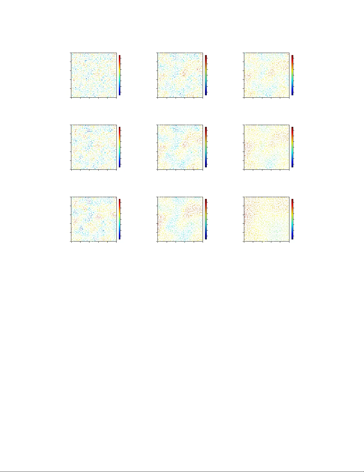
1 Lar ge-scale En vironmental Data Science with ExaGeoStatR Sameh Abdulah, Y uxiao Li, Jian Cao, Hatem Ltaief, David E. K e yes, Marc G. Genton, and Y ing Sun Computer , Electrical and Mathematical Sciences and Engineering Di vision, King Abdullah Uni versity of Science and T echnology (KA UST), Thuw al, Saudi Arabia Abstract Parallel computing in exact Gaussian process calculations becomes necessary for a voiding computa- tional and memory restrictions associated with large-scale en vironmental data science applications. The exact ev aluation of the Gaussian log-likelihood function requires O ( n 2 ) storage and O ( n 3 ) operations where n is the number of geographical locations. Thus, exactly computing the log-likelihood function with a large number of locations requires exploiting the power of existing parallel computing hardware systems, such as shared-memory , possibly equipped with GPUs, and distributed-memory systems, to solve this e xact computational complexity . In this paper , we present ExaGeoStatR , a package for exascale Geostatistics in R that supports a parallel computation of the exact maximum likelihood function on a wide v ariety of parallel architectures. Furthermore, the package allows scaling existing Gaussian process methods to a large spatial/temporal domain. Prohibitiv e exact solutions for large geostatistical problems become possible with ExaGeoStatR . Parallelization in ExaGeoStatR depends on breaking down the numerical linear algebra operations in the log-likelihood function into a set of tasks and rendering them for a task-based programming model. The package can be used directly through the R environment on parallel systems without the user needing any C , CUD A , or MPI knowledge. Currently , ExaGeoStatR supports sev eral maximum likelihood computation variants such as exact, Diagonal Super Tile (DST) and T ile Lo w-Rank (TLR) approximations, and Mix ed-Precision (MP). ExaGeoStatR also provides a tool to simulate large-scale synthetic datasets. These datasets can help assess different implementations of the maximum log-likelihood approximation methods. Herein, we show the implementation details of ExaGeoStatR , analyze its performance on v arious parallel architectures, and assess its accuracy using synthetic datasets with up to 250K observations. The experimental analysis cov ers the exact computation of ExaGeoStatR to demonstrate the parallel capabilities of the package. W e provide a hands-on tutorial to analyze a sea surface temperature real dataset. The performance e valuation in volv es comparisons with the popular packages GeoR , ﬁelds , and bigGP for exact Gaussian likelihood ev aluation. The approximation methods in ExaGeoStatR are not considered in this paper since they were analyzed in previous studies. Index T erms En vironmental application; Gaussian process; Matérn cov ariance function; maximum likelihood optimization; parameter estimation; prediction. 2 I . I N T R O D U C T I O N Massi ve data require a delicate analysis to extract meaningful information from their complex structure. W ith the a vailability of large data volumes coming from different sources, an objecti ve of data science is to combine a set of principles and techniques from data mining, machine learning, and statistics to support a better understanding of the giv en data. Like other sciences, en vironmental science has been very much impacted by the ﬁeld of data science. Indeed, a v ast pool of techniques has been dev eloped to understand spatial and spatio-temporal data coming from intelligent sensors or satellite images. Howe ver , new challenges hav e arisen with today’ s data sizes that require a unique treatment paradigm. En vironmental applications deal with measurements regularly or irregularly located across a geographical region. Gaussian processes (GPs), or Gaussian Random Fields (GRFs), are among the most useful tools in applications for ﬁtting spatial datasets. For the last two decades, GPs hav e been used extensi vely to model spatial data and are able to cover a wide range of spatial data with different speciﬁcations [Gelfand and Schliep, 2016]. Spatial data can also be described as random effects, hence they can often be modeled with a Gaussian distribution. Therefore, the dependencies in spatial data can be described through a Gaussian process. GRFs also serv e as building blocks for numerous non-Gaussian models in spatial statistics such as trans-Gaussian random ﬁelds, mixture GRFs and ske wed GRFs. For example, Xu and Genton [2017] introduced the T uke y g -and- h random ﬁeld which modiﬁes the GRF by a ﬂexible form of v ariable transformation; Andrews and Mallows [1974], W est [1987], and Rue and Held [2005] considered the scale-mixture of Gaussian distrib utions and GRFs; and Allard and Na veau [2007] and Azzalini [2005] proposed many ske wed GRFs and their variations. Howe ver , likelihood- based inference methods for GP models are computationally expensi ve for large-scale spatial datasets. It is crucial to pro vide fast computational tools to ﬁt a GP model to lar ge-scale spatial datasets often av ailable in many real-world applications. Speciﬁcally , suppose Z ( s ) is a stationary GRF with mean function m ( s ) and cov ariance 3 function C ( s , s 0 ) , and we observe data on a domain D ⊂ R d at n locations, s 1 , . . . , s n . Then, the random vector { Z ( s 1 ) , . . . , Z ( s n ) } > is assumed to follo w a multi variate Gaussian distribution: ∀{ s 1 , . . . , s n } ⊂ D , { Z ( s 1 ) , . . . , Z ( s n ) } > ∼ N n ( µ , Σ ) , (1) where µ = { m ( s 1 ) , . . . , m ( s n ) } > and Σ are the mean vector and the cov ariance matrix of the n -dimensional multiv ariate normal distribution. Giv en µ and Σ , the (Gaussian) likelihood of observing z = { z ( s 1 ) , . . . , z ( s n ) } > at the n locations is L ( µ , Σ ) = 1 (2 π ) n/ 2 | Σ | 1 / 2 exp  − 1 2 ( z − µ ) > Σ − 1 ( z − µ )  . (2) The ( i, j ) -th element of Σ is Σ ij = C ( s i , s j ) , where the covariance function C ( s i , s j ) is assumed to ha ve a parametric form with unknown vector of parameters θ . V arious classes of cov ariance functions can be found in e.g. Cressie [2015]. For simplicity , in this work, we assume the mean v ector µ to be zero to focus on estimating the covariance parameters. W e choose the most popular isotropic Matérn cov ariance kernel, which is speciﬁed as, Σ ij = C ( k s i − s j k ) = σ 2 2 ν − 1 Γ( ν )  k s i − s j k β  ν K ν  k s i − s j k β  , (3) where k s i − s j k is the Euclidean distance between s i and s j , Γ( · ) is the gamma function, K ν ( · ) is the modiﬁed Bessel function of the second kind of order ν , and σ 2 , β > 0 , and ν > 0 are the key parameters of the cov ariance function controlling the variance, spatial range, and smoothness, respectiv ely . The Matérn cov ariance kernel is highly ﬂexible and includes the exponential ( ν = 1 / 2 ) and Gaussian ( ν = ∞ ) kernels as special cases. The variance, spatial range, and smoothness parameters, σ 2 , β , and ν determine the properties of the GRF . The typical inference for GRFs includes parameter estimation, stochastic simulation, and kriging (spatial prediction). Among these tasks, parameter estimation, or model ﬁtting, is the most time-consuming. Once the parameters are estimated, one can easily simulate multiple 4 realizations of the GRF or obtain predictions at new locations. T o obtain the maximum like- lihood estimator (MLE), we need to optimize the likelihood function in Equation (2) ov er θ = ( σ 2 , β , ν ) > . Ho wev er , the likelihood for a given θ requires computing the in verse ( Σ ( θ ) − 1 ) and the determinant ( | Σ ( θ ) | ) of the cov ariance matrix Σ ( θ ) , and performing the triangular linear solve ( Σ ( θ ) − 1 Z ). The most time-consuming operation to compute the likelihood function is the Cholesky factorization for Σ ( θ ) , which requires O ( n 3 ) operations and O ( n 2 ) memory . This factorization is required to compute the in verse and the determinant of Σ ( θ ) . Due to the likelihood estimation complexity , the standard methods and traditional algorithms for GRFs are computationally infeasible for large datasets. On the other hand, technological advances in sensor networks along with the in vestments in data monitoring, collection, resource management provide massiv e open-access spatial datasets [Finley et al., 2015]. The unprecedented data av ailability and the challenging computational complexity call for novel methods, algorithms, and software packages to deal with modern “Big Data” problems in spatial statistics. A broad literature focuses on de veloping efﬁcient methodologies by approximating the cov ari- ance function in the GP model, so that the resulting cov ariance matrix is easier to compute. Sun et al. [2012], Bradley et al. [2016], and Liu et al. [2020] systematically revie wed these methods. Some popular approximation methods are cov ariance tapering [Furrer et al., 2006, Kaufman et al., 2008], discrete process con volutions [Higdon, 2002, Lemos and Sansó, 2009], ﬁx ed rank kriging [Cressie and Johannesson, 2008], lattice kriging [Nychka et al., 2015], and predictiv e processes [Banerjee et al., 2008, Finley et al., 2009]. Meanwhile, some studies proposed to approximate the Gaussian likelihood function using conditional distributions [Katzfuss and Guinness, 2021, V ecchia, 1988] or composite likelihoods [Eidsvik et al., 2014, V arin et al., 2011], and some seek for equiv alent representation of GPs using spectral density [Fuentes, 2007] and stochastic partial dif ferential equations [Lindgren et al., 2011]. A recent direction of this research aims at de veloping parallel algorithms [Datta et al., 2016, 5 Guhaniyogi and Banerjee, 2018, Katzfuss and Hammerling, 2017, Paciorek et al., 2015] and using modern computational architectures, such as multicore systems, GPUs, and supercomputers, in order to a void insuf ﬁcient approximation of the GP [Simpson et al., 2012, Stein, 2014]. Aggre gat- ing computing power through High-Performance Computing (HPC) becomes an important tool in scaling existing software in dif ferent disciplines to handle the e xponential gro wth of datasets generated in these ﬁelds [V etter, 2013]. Howe ver , the literature lacks a well-developed HPC software that practitioners can use to support their applications with HPC capabilities. Although most studies provide reproducible source codes, they are dif ﬁcult to extend to new applications, especially when the algorithms require certain hardware setups. R [Ihaka and Gentleman, 1996] is the most popular software in statistics, applied analytics, and interactiv e exploration of data by far . As a high-le vel language, ho we ver , R is relativ ely weak for high-performance computing compared to lo wer-le vel languages, such as C , C++ , and F ortr an . Scaling statistical software and bridging high-performance computing with the R language can be performed using two dif ferent strategies. One strategy has been follo wed by the pbdR [Ostrouchov et al., 2012] project, Programming with Big Data in R , which transfers the HPC libraries to the R en vironment by providing a high-lev el R interface to a set of HPC libraries such as MPI , ScaLAP A CK , Zer oMQ , to name a fe w . Howe ver , one drawback of this strategy is that the R dev eloper should hav e enough background in HPC to be able to use the provided interfaces to scale his/her code. Another strategy that we adopt in this paper is to implement the statistical functions using an HPC-friendly language such as C . Then it is easier to directly wrap the C functions into R functions. In this case, these functions can directly be used inside the R en vironment without the need to understand the underlying HPC architectures or the de velopment en vironment. This paper presents ExaGeoStatR , a high-performance package in R for large-scale en viron- mental data science and geostatistical applications that depends on a uniﬁed C -based software called ExaGeoStat [Abdulah et al., 2018a]. ExaGeoStat is able to ﬁt Gaussian process models and provide spatial predictions and simulations for geostatistics applications in large-scale domains. 6 ExaGeoStat provides both exact and approximate computations for large-scale spatial datasets. Besides the exact method, the software also supports three approximation methods: Diagonal Super T ile (DST), Tile Lo w-Rank (TLR), and Mixed-Precision (MP) computations. This study highlights the capabilities of the ExaGeoStatR exact computations since it can be considered a benchmark for the performance of other computation methods. Moreover , the ev aluation of the DST and the TLR approximations has already been cov ered in Abdulah et al. [2018a,b, 2019, 2022b], Hong et al. [2021]. The software also includes a synthetic dataset generator for generating large spatial datasets with the exact prespeciﬁed cov ariance function. Such large datasets can be used to perform broader scientiﬁc e xperiments related to large-scale computational geostatistics applications. Besides its ability to deal with different hardware architectures such as multicore systems, GPUs, and distrib uted systems, ExaGeoStatR utilizes the underlying hardware architec- tures to its full extent. Existing assessments on ExaGeoStat show the ability of the software to handle up to 3.4 million spatial locations on manycore systems with exact calculations [Abdulah et al., 2022b]. Existing R packages for ﬁtting GRFs include GeoR [Ribeiro Jr and Diggle, 2016], ﬁelds [Nychka et al., 2017], spBayes [Finley et al., 2007a, 2015], RandomF ields [Schlather et al., 2015a, 2019], INLA [Martins et al., 2013, Rue et al., 2009], bigGP [Paciorek et al., 2015]. These packages feature different degrees of ﬂexibility as well as computational capacity . The spBayes package ﬁts GP models in the context of Bayesian or hierarchical modeling based on MCMC. The RandomF ields package implements the Cholesky factorization method, the circulant embedding method [Dietrich and Newsam, 1996], and an extended version of Matheron’ s turning bands method [Matheron, 1973] for the maximum likelihood estimation of GRFs. The INLA package uses an integrated nested Laplace approximation to tackle additi ve models with a latent GRF , which outperforms the MCMC method. The bigGP package utilizes distributed memory systems through RMPI [Gropp et al., 1999] to implement the estimation, prediction, and simulation of GRFs. The packages GeoR and ﬁelds both estimate the GRF co variance structures designed for 7 spatial statistics while GeoR pro vides more ﬂexibilities, such as estimating the mean structure and the variable transformation parameters. Among these popular packages, only the bigGP package, according to our knowledge, focuses on distributed computing, which is essential for solving problems in data-rich en vironments in exact mode. The bigGP package was built using the RMPI and OpenMP libraries to facilitate GP calculations on manycore systems. The bigGP package relies on block-based algorithms to perform the underlying linear algebra operations required to perform the GP calculations. Compared to the bigGP package, ExaGeoStatR provide better performance since it depends on the state-of-the-art parallel linear algebra operations through applying tile-based algorithms to perform the required linear solvers. T able I provides a summary of some of the existing packages for ﬁtting GRFs. The comparison includes common features for each package and if it supports parallel ex ecution or not. Our package ExaGeoStatR , at the current stage, performs data generation, parameter estima- tion, and spatial prediction for the univ ariate GRF with mean zero and a Matérn covariance structure, which is a fundamental model in spatial statistics. W e feature breakthroughs in the optimization routine for the maximum likelihood estimation and the utilization of heterogeneous computational units. Speciﬁcally , we build on the optimization library NLopt [Johnson, 2014] and provide a uniﬁed Application Programming Interface (API) for multicore systems, GPUs, clusters, and supercomputers. The package also supports using the great circle distance on the sphere in constructing the cov ariance matrix. These parallelization features largely reduce the time-per-iteration in computing exact maximum likelihood estimations compared with existing packages and make GRFs ev en with 10 6 locations estimable on hardware accessible to most institutions. The remainder of this paper is org anized as follo ws. Section II states the basics of Exa- GeoStatR , and the package components for keen readers. Section III compares the estimation accuracy and time of ExaGeoStatR with two aforementioned exact computation packages, i.e., GeoR and ﬁelds , with simulated data. It demonstrates the efﬁcienc y that can be gained when the 8 ExaGeoStatR package utilizes powerful architectures including GPUs and distributed memory systems. Section IV is a tutorial to ﬁt a Gaussian random ﬁeld to a sea surface temperature dataset with more than ten thousand spatial locations per day and perform kriging with the estimated parameter values. Section V concludes with the contributions of the ExaGeoStatR package. In the Appendix, we provide a user guide for installing the ExaGeoStatR package on dif ferent hardware en vironments. I I . S O F T W A R E O V E RV I E W A. ExaGeoStat Outline ExaGeoStat 1 is a C -based software that targets en vironmental applications through a high- performance parallel implementation of the Maximum Likelihood Estimation (MLE) operation that is widely used for geospatial statistics [Abdulah et al., 2018a]. This software provides a nov el solution to deal with the scaling limitation impact of the MLE operation by exploiting the computational power of emerging hardware architectures. ExaGeoStat permits exploring the MLE computational limits using state-of-the-art high-performance dense linear algebra libraries by lev eraging a single source code to run on v arious cutting-edge parallel architectures with the aide of runtime systems software. The “separation of concerns” philosophy adopted by ExaGeoStat from the beginning permits improving the software from different perspectiv es by allo wing fast linear solvers and porting the code to different hardware architectures. ExaGeoStat is dev eloped to solve the MLE problem for a giv en set of data observed at n geographical locations on a large scale and to provide a prediction solution for unobserved values at ne w locations. The software also allows for exact synthetic data generations with a giv en cov ariance function, which can be used to test and compare dif ferent approximation methods. T o sum up, ExaGeoStat includes three primary tools: large-scale synthetic data generator , the Gaussian maximum likelihood estimator , and the geospatial predictor . 1 https://github .com/ecrc/exageostat 9 In ExaGeoStat , the MLE operation is implemented in four different ways: Fully-Dense (Exact), Diagonal Super T ile (DST) [Abdulah et al., 2018a], T ile Low-Rank (TLR) [Abdulah et al., 2018b], and mixed-precision [Abdulah et al., 2019, 2022b]. The four different implementations rely on state-of-the-art parallel algebraic computations by exploiting adv ances in algorithmic solutions and manycore computer architectures. The parallel implementation consists in di viding the gi ven co variance matrix into a set of small tiles where a single processing unit can process a single tile at a time. The main difference between different implementations is the structure of the underlying cov ariance matrix. In dense computation, matrix tiles are represented in fully double-precision format as sho wn by Figure 1 (a). The provided solution is exact but with the cost of more computing power and storage space. The DST implementation depends on annihilating some of the of f-diagonal tiles because their contributions and qualitati ve impact on the overall statistical problem may be limited while depending on diagonal tiles, which should hav e a stronger inﬂuence on the underlying model. Choosing the number of tiles to be ignored is up to the user who should expect losing some accuracy with more zero tiles. Figure 1 (b) depicts the cov ariance matrix in the case of DST representation where two-diagonal tiles are represented in dense format while all the other tiles are set to zero. The TLR implementation depends on representing the tiles in lo w-rank format. Currently , ExaGeoStat supports the Singular V alue Decomposition (SVD) technique to compress the off-diagonal tiles in low-rank while other compression methods exist in the literature. The TLR computation depends on the TLR linear algebra operations that can pro vide fast computation with appropriate accuracy . In Figure 1 (c), the TLR approximation method is used where the k most signiﬁcant singular values/v ectors are captured for each of f-diagonal tile to maintain the overall ﬁdelity of the numerical model depending on the application-speciﬁc accuracy . Finally , the mixed-precision implementation is inspired by the DST approximation technique. Instead of ignoring some of f-diagonal tiles and setting their elements as zero, ExaGeoStat represents their elements in lo wer-precision, i.e., single or half. In this case, we can speed up the computation compared to the fully-dense 10 (a) Fully dense (Exact) (b) Diag. Super-T ile (DST) (c) T ile Low-Rank (TLR) Ze ro Ti l e s Den s e Ti l e s Si n g l e P re ci si o n Do u b l e Pr ec i s i o n SP Tiles DP Tiles HP Tiles (d) Mixed-Precision (MP) Fig. 1: ExaGeoStat supports various computation methods. The tile is a subset of the matrix with size ts × ts . Here ts should be tuned for performance on parallel systems. DP refers to double- precision (64-bit) tile, SP refers to single-precision (32-bit) tile, and HP refers to half-precision (16-bit) tile. implementation b ut with higher accuracy than the DST approximation. Figures 1 (d) depicts the mixed-precision cov ariance matrix structure supported by ExaGeoStat . B. The ExaGeoStat Infrastructur e T o provide the different computational variants sho wn abov e, ExaGeoStat internally relies on three parallel linear algebra libraries to construct the basic linear algebra operations for the MLE computation. Exact, DST , and mixed-precision approximation computations rely on the Chameleon library , a high-performance numerical library that provides high-performance dense linear solvers [cha, 2022] or the DPLASMA library , dense linear algebra algorithms on massiv ely parallel architectures [Bosilca et al., 2011]. The TLR approximation computation depends on the HiCMA library , a hierarchical linear algebra library on manycore architectures, that provides parallel approximation solvers [Abdulah et al., 2022a]. The HiCMA is associated with the ST ARS- H library , a high-performance H -matrix generator library on large-scale systems, which provides test cases for the HiCMA library [sta, 2022]. Both Chameleon and HiCMA libraries provide linear algebra operations through a set of sequential task-based algorithms. For hardware portability , ExaGeoStat features the StarPU [Augonnet et al., 2011] and P aRSEC [Bosilca et al., 2013] dynamic runtime systems as backends. The runtime system proposes a kind of abstraction to improv e the user’ s producti vity and creati vity . For example, Chameleon 11 and HiCMA provide sequential task-based linear algebra operations through a sequential task ﬂo w (STF) programming model. StarPU is able to execute the set of giv en sequential tasks in parallel with giv en hints of the data dependencies (e.g., read, write, and read-write). The main advantage of using runtime systems that rely on task-based implementations is becoming obli vious to the targeted hardware architecture. Multiple implementations of the same tasks are generated for: CPU, CUDA, OpenCL, OpenMP , and MPI, to name a fe w . T o achie ve the highest performance, the runtime system decides which implementation will achiev e the highest performance at runtime. For the ﬁrst execution, the runtime system generates a set of cost models that determine the best hardware for optimal performance during the gi ven tasks. This set of cost models may be sav ed for future ex ecutions. The top layer of ExaGeoStat is the optimization toolbox. ExaGeoStat relies on an open-source C / C ++ nonlinear optimization toolbox, NLopt [Johnson, 2014], to perform the MLE optimization operation. Among 20 global and local optimization algorithms supported by the NLopt library , we selected the Bound Optimization BY Quadratic Approximation (BOBYQA) algorithm to be our optimization algorithm. BOBYQA performs well with our target nonlinear problem with a global maximum point. BOBYQA is a numeric, global, deriv ativ e-free, and bound-constrained optimization algorithm. It generates a ne w computed point on each iteration by solving a trust- region subproblem subject to giv en constraints. In ExaGeoStat , only upper and lower bound constraints are used. Though BOBYQA does not require e valuating the deriv ativ es of the cost function, it iterati vely employs an updated quadratic model of the objectiv e, so there is an implicit assumption of smoothness. In summary , ExaGeoStat relies on a set of software that expands the software portability capabilities. Figure 2 sho ws the ExaGeoStat infrastructure with four main layers: the BOBYQA algorithm from the NLopt library for optimization purpose; the log-likelihood estimation upper- le vel operation; the Chameleon / HiCMA / DPLASMA libraries, which provide exact (the focus of this study) and approximate solvers for the linear algebra operations using task-based parallel 12 algorithms; and the StarPU / P aRSEC dynamic runtime systems, which translate the software for ex ecution on the appropriate underlying hardware. T able II summarizes the complete list of software dependencies. An optimized BLAS library should be av ailable based on the hardware architecture, e.g., Intel MKL for CPU and OpenBLAS for GPU. The hwloc library is used to abstract the underlying hardware topology to the runtime system. In contrast, the GSL library provides a vast set of numerical functions that are needed by some of the cov ariance functions. For instance, the Bessel and gamma functions for the Matérn cov ariance function. BOBYQA Optimization Algorithm Log -Likelihood Estimation Task-based Linear Algebra Solvers Dynamic Runtime System Parallel Hardware Architectures Shared Memory Systems Distributed Memo ry Systems GPUs StarPU PaRSEC Chameleon HiCMA DPLASMA NLopt STARS-H Fig. 2: ExaGeoStat infrastructure. C. ExaGeoStatR P ackag e T o facilitate the use of large-scale ex ecutions in the R en vironment, we present a package in R , i.e., ExaGeoStatR 2 , on top of our ExaGeoStat software that provides high-performance geospatial statistics functions in R . This package in R should help disseminate our software to a large computational and spatial statistics community . T o the best of our knowledge, most of the existing R solutions for the MLE problem are sequential and restricted to limited data sizes. A fe w of them depend on running on multiple cores within the same shared memory system by enabling OpenMP support. ExaGeoStatR targets all the existing parallel hardware architectures, 2 https://github .com/ecrc/exageostatR 13 including GPUs and distrib uted memory systems, with a high-lev el abstraction of the underlying hardware architecture for the user . T able III gi ves an overvie w of current ExaGeoStatR functions with a description of their main operations. W e provide an ExaGeoStatR installation tutorial in the Appendix. I I I . S I M U L A T I O N S T U D I E S In this section, we provide a set of examples with associated code to better understand the ExaGeoStatR package. The examples possess three goals: 1) provide step-by-step instructions of using ExaGeoStatR on multiple different tasks; 2) assess the performance and accuracy of the proposed exact computation compared to existing R packages; and 3) assess the performance of the ExaGeoStatR package using different hardware architectures. All the upcoming experiments rely on the Chameleon linear algebra library and StarPU runtime system when ex ecuting the ExaGeoStatR functions. A. P erformance Evaluation of ExaGeoStatR The performance of ExaGeoStatR is e valuated on various systems: the experiments in Exam- ples 1 and 2 below are implemented on a Ubuntu 16.04.5 L TS workstation with a dual-socket 8-core Intel Sandy Bridge Intel Xeon E5-2650 without any GPU acceleration; Example 3 is assessed on a dual-socket 14-core Intel Broadwell Intel Xeon CPU E5-2680 v3 running at 2.40 GHz and equipped with 8 NVIDIA K80s (2 GPUs per board), and Example 4 is tested on KA UST’ s Cray XC40 supercomputer system, Shaheen II, with 6174 nodes, each node is dual- socket 16-core Intel Haswell processor running at 2.30 GHz and 128 GB of DDR4 memory , and Example 5 is tested on KA UST Ibex cluster with up to 16 nodes. T wo popular R packages, GeoR [Ribeiro Jr and Diggle, 2016] and ﬁelds [Nychka et al., 2017], are selected as our references for exact computations. 14 Since ExaGeoStatR works with multiple cores and different hardware architectures, users need to initialize their preferred settings using the exag eostat_init function. When users want to change or terminate the current hardware allocation, the e xageostat_ﬁnalize function is required: > library ( " e x a g e o s t a t r " ) > h a r d w a r e = list ( n c o r e s = 2 , n g p u s = 0 , ts = 3 2 0 , p g r i d = 1 , q g r i d = 1 ) > e x a g e o s t a t _ i n i t ( h a r d w a r e ) > e x a g e o s t a t _ f i n a l i z e ( ) The har dwar e = list() speciﬁes the required hardware to ex ecute the code. Here, ncores and ngpus are the numbers of CPU cores and GPU accelerators to deploy , ts denotes the tile size used for parallelized matrix operations, pgrid and qgrid are the cluster topology parameters in case of distributed memory system execution. B. P erformance Optimization Options In general, the performance of the ExaGeoStatR package on shared memory , GPUs, and distributed memory systems can be optimized by explicitly using StarPU optimization en vi- ronment variables. For example, the ST ARPU_SCHED environment variable is used to select appropriate parallel tasks scheduling policies provided by StarPU , such as random, eager , and stealing. It determines how to distribute individual tasks to dif ferent processing units. The user needs to try various schedulers to satisfy the best performance on the target hardware. Other examples of en vironment variables are ST ARPU_LIMIT_MAX_SUBMITTED_T ASKS and ST ARPU_LIMIT_MIN_SUBMITTED_T ASKS which control the number of submitted tasks and enable cache buf fer reuse in main memory . C. Example 1: Data Generation ExaGeoStatR of fers two functions to generate realizations from Gaussian random ﬁelds with zero mean and Matérn cov ariance function shown in Equation (3). The simulate_data_exact function generates a GRF at a set of irregularly spaced random locations. Fi ve inputs need to be 15 gi ven. The k ernel input accepts one of se ven co variance functions: uni variate Gaussian stationary Matérn - space ( ugsm-s ), bi variate Gaussian stationary ﬂe xible Matérn - space ( bgsfm-s ), bi variate Gaussian stationary parsimonious Matérn - space ( bgspm-s ), triv ariate Gaussian stationary parsi- monious Matérn - space ( tgspm-s ), univ ariate Gaussian stationary Matérn - space-time ( ugsm-st ), and bi variate Gaussian stationary Matérn - space-time ( bgsm-st ). T able IV summarizes the current cov ariance functions supported by ExaGeoStatR . The theta input is a vector of the initial model parameters used to generate the simulated target geospatial dataset. The theta vector length depends on the chosen k er nel . The dmetric input accepts two values: euclidean for Euclidean distance or great_cir cle for great circle distance in case of spherical data [V eness, 2010]. The n input accepts the number of geospatial locations of the generated data in the unit square as mentioned in Abdulah et al. [2018a]. The code below gi ves a simple example of generating a realization from a uni v ariate Gaussian stationary random ﬁeld at 1600 random locations using the simulate_data_exact function: > h a r d w a r e = list ( n c o r e s = 4 , n g p u s = 0 , ts = 3 2 0 , p g r i d = 1 , q g r i d = 1 ) > e x a g e o s t a t _ i n i t ( h a r d w a r e ) > d a t a . e x a g e o . i r r e g = s i m u l a t e _ d a t a _ e x a c t ( k e r n e l = " u g s m − s " , t h e t a = c ( 1 , 0 . 1 , 0 . 5 ) , d m e t r i c = " e u c l i d e a n " , n = 1 6 0 0 , s e e d = 0 ) > e x a g e o s t a t _ f i n a l i z e ( ) The code starts with deﬁning the hardware resources which will be used to run the e xample. The second line initiates a new ExaGeoStatR instance. The third line simulates synthetic data using a gi ven cov ariance function with a giv en parameter vector . Finally , the last line closes the activ e ExaGeoStatR instance. The results are stored as a list, data=list{x,y ,z} , where x and y are coordinates, and z stores the simulated realizations. Here, x and y are generated from a uniform distrib ution on [0 , 1] . Therefore, the generated locations are irregular on [0 , 1] × [0 , 1] with simulate_data_exact function. T o generate data on a regular grid, outside the range of [0 , 1] × [0 , 1] , or at speciﬁc locations, one can use the simulate_obs_exact function by providing the coordinates x and y . The following code shows an example of generating a GRF on a 16 [0 , 2] × [0 , 2] spatial grid with 1600 locations: > h a r d w a r e = list ( n c o r e s = 2 , n g p u s = 0 , ts = 3 2 0 , p g r i d = 1 , q g r i d = 1 ) > e x a g e o s t a t _ i n i t ( h a r d w a r e ) > xy = expand . grid ( ( 1 : 4 0 ) / 2 0 , ( 1 : 4 0 ) / 2 0 ) > x = xy [ , 1 ] > y = xy [ , 2 ] > d a t a . e x a g e o . r e g = s i m u l a t e _ o b s _ e x a c t ( x = x , y = y , k e r n e l = " u g s m − s " , t h e t a = c ( 1 , 0 . 1 , 0 . 5 ) , d m e t r i c = " e u c l i d e a n " ) > e x a g e o s t a t _ f i n a l i z e ( ) Line 5 in the code simulates synthetic data on giv en 2d locations using a predeﬁned cov ariance function and a gi ven parameter vector . In Figure 3, some examples of data simulated using the ExaGeoStatR package at 1600 locations in the unit square using the univ ariate Matérn stationary cov ariance function. The data was generated using seed = 1 . For comparison purpose, we also show how the sim.rf function of ﬁelds and the grf function of GeoR generate similar GRFs: > library ( g e o R ) > s i m s = g r f ( n = 1 6 0 0 , grid = " r e g " , cov . p a r s = c ( 1 , 0 . 1 ) , kappa = 0 . 5 ) > d a t a . g e o R . r e g = list ( x = s i m s $coords [ , 1 ] , y = s i m s $coords [ , 2 ] , z = s i m s $ d a t a ) > library ( fields ) > s i g m a _ s q = 1 > grid = list ( x = ( 1 : 4 0 ) / 2 0 , y = ( 1 : 4 0 ) / 2 0 ) > xy = expand . grid ( x = ( 1 : 4 0 ) / 2 0 , y = ( 1 : 4 0 ) / 2 0 ) > o b j = m a t e r n . image . cov ( grid = grid , t h e t a = 0 . 1 , s m o o t h n e s s = 0 . 5 , s e t u p = T R U E ) > s i m s . fields = sqrt ( s i g m a _ s q ) * s i m . rf ( o b j ) > d a t a . fields . r e g = list ( x = xy [ , 1 ] , y = xy [ , 2 ] , z = c ( s i m s . fields ) ) As can be seen, the three packages of fer different types of ﬂexibility in terms of data gener- ation. Howe ver , when the goal is to generate a large GRF on an irregular grid with more than 20 K locations, both the sim.rf function and the grf function are not feasible. The sim.rf function simulates a stationary GRF only on a regular grid, and the grf function shows memory issues 17 0.0 0.2 0.4 0.6 0.8 1.0 0.0 0.2 0.4 0.6 0.8 1.0 −3 −2 −1 0 1 2 3 (a) (1, 0.03, 0.5) 0.0 0.2 0.4 0.6 0.8 1.0 0.0 0.2 0.4 0.6 0.8 1.0 −3 −2 −1 0 1 2 3 (b) (1, 0.1, 0.5) 0.0 0.2 0.4 0.6 0.8 1.0 0.0 0.2 0.4 0.6 0.8 1.0 −3 −2 −1 0 1 2 3 (c) (1, 0.3, 0.5) 0.0 0.2 0.4 0.6 0.8 1.0 0.0 0.2 0.4 0.6 0.8 1.0 −3 −2 −1 0 1 2 3 (d) (1, 0.03, 1) 0.0 0.2 0.4 0.6 0.8 1.0 0.0 0.2 0.4 0.6 0.8 1.0 −3 −2 −1 0 1 2 3 (e) (1, 0.1, 1) 0.0 0.2 0.4 0.6 0.8 1.0 0.0 0.2 0.4 0.6 0.8 1.0 −3 −2 −1 0 1 2 3 (f) (1, 0.3, 1) 0.0 0.2 0.4 0.6 0.8 1.0 0.0 0.2 0.4 0.6 0.8 1.0 −3 −2 −1 0 1 2 3 (g) (1, 0.03, 2) 0.0 0.2 0.4 0.6 0.8 1.0 0.0 0.2 0.4 0.6 0.8 1.0 −3 −2 −1 0 1 2 3 (h) (1, 0.1, 2) 0.0 0.2 0.4 0.6 0.8 1.0 0.0 0.2 0.4 0.6 0.8 1.0 −3 −2 −1 0 1 2 3 (i) (1, 0.3, 2) Fig. 3: Data simulated using ExaGeoStatR with univ ariate Matérn stationary cov ariance function in ( σ 2 , β , ν ) form at 1600 geospatial locations in the unit square. for large size ( i.e., Err or:vector memory exhausted ). On the other hand, the simulate_data_exact function can easily generate the GRF within one minute with the follo wing code: > n = 2 5 6 0 0 > h a r d w a r e = list ( n c o r e s = 4 , n g p u s = 0 , ts = 3 2 0 , p g r i d = 1 , q g r i d = 1 ) > e x a g e o s t a t _ i n i t ( h a r d w a r e ) > d a t a . e x a g e o . r e g = s i m u l a t e _ d a t a _ e x a c t ( k e r n e l = " u g s m − s " , t h e t a = c ( 1 , 0 . 1 , 0 . 5 ) , d m e t r i c = " e u c l i d e a n " , n , s e e d = 0 ) > e x a g e o s t a t _ f i n a l i z e ( ) Simulating data on a large scale requires enough memory and computation resources. Thus, we recommend the users be consistent when generating large datasets with the a vailable hardware 18 resources. W e also provide a set of synthetic and real large spatial data examples that can be downloaded from https://ecrc.github .io/exageostat/md_docs_examples.html for experimental needs. D. Example 2: P erformance on Shar ed Memory Systems for Moderate and Lar ge Sample Size T o in vestigate the estimation of parameters based on the exact computation, we use the exact_mle function in ExaGeoStatR . On a shared memory system with a moderate sample size, the number of cores ( ncor es ) and tile size ( ts ) signiﬁcantly af fect the performance (see Figure 4). The following code shows the usage of the exact_mle function and returns execution time per iteration for one combination of n , ncor es and ts : > h a r d w a r e = l i s t ( n c o r e s = 4 , n g p u s = 0 , ts = 1 6 0 , p g r i d = 1 , q g r i d = 1 ) > e x a g e o s t a t _ i n i t ( h a r d w a r e ) > d a t a . e x a g e o . r e g = s i m u l a t e _ d a t a _ e x a c t ( k e r n e l = " u g s m − s " , t h e t a = c ( 1 , 0 . 1 , 0 . 5 ) , d m e t r i c = " e u c l i d e a n " , n = 1 6 0 0 , s e e d = 0 ) > r e s u l t = e x a c t _ m l e ( d a t a . e x a g e o . r e g , k e r n e l = " u g s m − s " , d m e t r i c = " e u c l i d e a n " , o p t i m i z a t i o n = l i s t ( c l b = c ( 0 . 0 0 1 , 0 . 0 0 1 , 0 . 0 0 1 ) , c u b = c ( 5 , 5 , 5 ) , t o l = 1 e − 4 , m ax _ i t e r s = 2 0 ) ) > t i m e = r e s u l t $ t i m e _ p e r _ i t e r > e x a g e o s t a t _ f i n a l i z e ( ) In the exact_mle function, the ﬁrst argument, data = list{x, y , z} , is a list that deﬁnes a set of locations in two-dimensional coordinates, x and y , and the measurement z of the variable of interest. The k er nel input deﬁnes the required cov ariance function. Here, dmetric is a distance parameter , the same as in the simulate_data_exact function. The optimization list speciﬁes the optimization settings including the lower and upper bounds vectors, clb and cub , tol is the optimization tolerance and max_iters is the maximum number of iterations to terminate the optimization process. The optimization function uses the clb vector as the starting point of the optimization. The above example has been ex ecuted using three different sample sizes, 16 different numbers of cores, and four dif ferent tile sizes to assess the parallel ex ecution performance of ExaGeoStatR . 19 W e visualize the results by using the ggplot function in ggplot2 [W ickham, 2016] as shown in Figure 4. The ﬁgure shows the computational time for the estimation process using a different number of cores up to 16 cores. The y-axis shows the total computation time per iteration in seconds, while the x-axis represents the number of cores. The three sub-ﬁgures sho w the performance with different n v alues: 400, 900, and 1600. Different curves represent different tile sizes which impact the performance of different hardware architectures. The ﬁgure shows that on our Intel Sandy Bridge machine, the best-selected tile size is 100. T iling helps parallel ex ecution to achie ve the highest performance by increasing the reuse of data already loaded from the main memory (RAM) to the processor cache and reducing the data mov ements from RAM to cache. So, obtaining the best tile size depends on the processor cache size. Moving a complete tile from RAM to cache should increase the computation ef ﬁciency of the underlying algorithm. Ho wev er , small tiles can also impact performance by satisfying better load balancing between the running processes, making determining the best tile size tricky . The simplest way to obtain the best tile size is to tune it on ne w hardware architectures before running large problems. W e recommend trying different tile sizes to get the best performance from the ExaGeoStatR package. After specifying the hardware en vironment settings, we test the accuracy of the likelihood- based estimation of ExaGeoStatR in comparison with GeoR and ﬁelds . The counterparts to the exact_mle function are likﬁt in GeoR and spatialPr ocess in ﬁelds . The simulated datasets from Example 1 are used as the input to assess the performance of parameter estimations. The synthetic datasets are generated on n=1600 points in [0 , 1] × [0 , 1] . W e take a moderate sample size that costs GeoR and ﬁelds approximately ten minutes to obtain enough results with dif ferent scenarios and iterations. The mean structure is assumed to be constantly zero across the region. One hundred replicates of samples are generated with different seed ( seed = 1 , . . . , 100 ) to quantify the uncertainty . W e estimate the parameter values for each sample and obtain 100 sets of estimates independently . A Matérn cov ariance kernel is selected to generate the cov ariance matrix 20 n: 1600 n: 400 n: 900 1 2 3 4 5 6 7 8 9 10 11 12 13 14 15 16 1 2 3 4 5 6 7 8 9 10 11 12 13 14 15 16 1 2 3 4 5 6 7 8 9 10 11 12 13 14 15 16 1 2 3 4 5 6 7 8 9 10 11 12 13 14 15 16 1 2 3 4 5 6 7 8 9 10 11 12 13 14 15 16 1 2 3 4 5 6 7 8 9 10 11 12 13 14 15 16 1 2 3 4 5 6 7 8 9 10 11 12 13 14 15 16 1 2 3 4 5 6 7 8 9 10 11 12 13 14 15 16 1 2 3 4 5 6 7 8 9 10 11 12 13 14 15 16 1 2 3 4 5 6 7 8 9 10 11 12 13 14 15 16 1 2 3 4 5 6 7 8 9 10 11 12 13 14 15 16 1 2 3 4 5 6 7 8 9 10 11 12 13 14 15 16 1 2 3 4 5 6 7 8 9 10 11 12 13 14 15 16 1 2 3 4 5 6 7 8 9 10 11 12 13 14 15 16 1 2 3 4 5 6 7 8 9 10 11 12 13 14 15 16 1 2 3 4 5 6 7 8 9 10 11 12 13 14 15 16 1 2 3 4 5 6 7 8 9 10 11 12 13 14 15 16 1 2 3 4 5 6 7 8 9 10 11 12 13 14 15 16 1 2 3 4 5 6 7 8 9 10 11 12 13 14 15 16 1 2 3 4 5 6 7 8 9 10 11 12 13 14 15 16 1 2 3 4 5 6 7 8 9 10 11 12 13 14 15 16 1 2 3 4 5 6 7 8 9 10 11 12 13 14 15 16 1 2 3 4 5 6 7 8 9 10 11 12 13 14 15 16 1 2 3 4 5 6 7 8 9 10 11 12 13 14 15 16 1 2 3 4 5 6 7 8 9 10 11 12 13 14 15 16 1 2 3 4 5 6 7 8 9 10 11 12 13 14 15 16 1 2 3 4 5 6 7 8 9 10 11 12 13 14 15 16 1 2 3 4 5 6 7 8 9 10 11 12 13 14 15 16 1 2 3 4 5 6 7 8 9 10 11 12 13 14 15 16 1 2 3 4 5 6 7 8 9 10 11 12 13 14 15 16 1 2 3 4 5 6 7 8 9 10 11 12 13 14 15 16 1 2 3 4 5 6 7 8 9 10 11 12 13 14 15 16 1 2 3 4 5 6 7 8 9 10 11 12 13 14 15 16 1 2 3 4 5 6 7 8 9 10 11 12 13 14 15 16 1 2 3 4 5 6 7 8 9 10 11 12 13 14 15 16 1 2 3 4 5 6 7 8 9 10 11 12 13 14 15 16 0.25 0.50 0.75 0.1 0.2 0.3 0.5 1.0 1.5 2.0 Number of CPU cores Execution time per iteration (s) ts 560 320 160 100 Fig. 4: Parallel ex ecution performance of ExaGeoStatR under different hardware settings. Each subﬁgure corresponds to a single sample size n and shows the execution time in seconds per iteration with regards to the number of cores up to 16. Curves with dif ferent colors provide the ef fect of tile size ( ts ). (Red: ts=100 . Green: ts=160 . Blue: ts=320 . Purple: ts=560 ). with nine different scenarios. Speciﬁcally , the variance is alw ays chosen to be one, sigma_sq = 1.0 , the spatial range takes three different v alues representing high, medium, and low spatial correlation, beta = c(0.3, 0.1, 0.03) , and the smoothness also takes three values from rough to smooth, nu = c(0.5, 1, 2) . The simulated datasets with moderate sample size are generated by the grf function. W e choose the grf function in GeoR due to its ﬂexibility in changing the parameter settings and in switching between regular and irregular grids. Herein, we depend on irregular grids to generate the data. W e set the absolute tolerance to 10 − 5 and unset the maximum number of iterations ( max_iters = 0 ) to avoid non-optimized results. Hence, each package can show its best performance to estimate the correct v alue of each parameter . The simulated GRFs are generated by the grf function and stored as a list called data : > library ( g e o R ) > s i g m a _ s q = 1 > b e t a = 0 . 1 # choose one from c(0.3, 0.1, 0.03) > n u = 0 . 5 # choose one fr om c(0.5, 1, 2) 21 > s i m s = g r f ( n = 1 6 0 0 , grid = " r e g " , cov . p a r s = c ( s i g m a _ s q , b e t a ) , kappa = n u ) > d a t a = list ( x = s i m s $coords [ , 1 ] , y = s i m s $coords [ , 2 ] , z = s i m s $ d a t a ) W e hav e tried to keep the irrelev ant factors as consistent as possible when comparing Ex- aGeoStatR with GeoR and ﬁelds . Ho wev er , we identiﬁed some differences between the three packages that can hardly be reconciled. For example, GeoR estimates the mean structure together with the cov ariance structure, and ﬁelds does not estimate the smoothness parameter , ν , in our package. In addition, in terms of the optimization methods, both GeoR and ﬁelds call the optim function in stats to maximize the likelihood function. The optim function includes six methods such as Nelder-Mead and BFGS . Howe ver , ExaGeoStatR uses the BOBYQA algorithm, which is one of the optimization algorithms of the sequential NLopt library in C/C++ . The BOBYQA algorithm has the best performance in terms of MLE estimation. Howe ver , it is not av ailable in the optim function. T able V lists the dif ferences between the three packages. Multiple algorithms are of fered by the optim function and further implemented by GeoR and ﬁelds . Howe ver , many studies in the literature point out that the optim function is not numerically stable for a large number of mathematical functions, especially when a re-parameterization exists [Mullen et al., 2014, Nash et al., 2011, 2014]. Based on the 100 simulated samples, we sho w that ExaGeoStatR provides faster computation and gi ves more accurate and robust estimations with regards to the initial value and grid type. W e ﬁrst estimate the parameters by exact_mle in ExaGeoStatR . W e use the number of cores to be eight to reproduce the results on most machines. Users can specify their settings and optimize the performance by referring to the results in Figure 4. The ﬁnal results also report the time per iteration, total time, and the number of iterations for each optimization: > h a r d w a r e = list ( n c o r e s = 8 , n g p u s = 0 , ts = 1 0 0 , p g r i d = 1 , q g r i d = 1 ) > e x a g e o s t a t _ i n i t ( h a r d w a r e ) > r e s u l t = e x a c t _ m l e ( d a t a , k e r n e l = " u g s m − s " , d m e t r i c = " e u c l i d e a n " , o p t i m i z a t i o n = list ( c l b = c ( 0 . 0 0 1 , 0 . 0 0 1 , 0 . 0 0 1 ) , c u b = c ( 5 , 5 , 5 ) , t o l = 1 e − 4 , max_ i t e r s = 2 0 ) ) > p a r a _mat = r e s u l t $ e s t _ t h e t a 22 > time_mat = c ( r e s u l t $time_ p e r _ i t e r , r e s u l t $ t o t a l _time , r e s u l t $ n o _ i t e r s ) > e x a g e o s t a t _ f i n a l i z e ( ) Then we estimate the parameters under the same scenarios using the likﬁt function in GeoR and the spatialPr ocess function in ﬁelds . For GeoR and ﬁelds , the chosen optimization options are method = c("Nelder-Mead") , abstol = 1e-5 , and maxit = 500 , where the maximum number of iterations set as 500 could never be reached. Because ﬁelds does not optimize the smoothness, ν , so we set it as the true value (an adv antageous fav or for ﬁelds ). GeoR has to optimize the mean parameter , at least a constant, but it is treated to be independent of the cov ariance parameters as the mean v alue of data. In addition, to accelerate the optimization of ﬁelds , we minimize the irrele vant computation by setting gridN = 1 : > r e s u l t = s p a t i a l P r o c e s s ( x = cbind ( d a t a $ x , d a t a $ y ) , y = d a t a $ z , cov . args = list ( C o v a r i a n c e = " M a t e r n " , s m o o t h n e s s = n u ) , g r i d N = 1 , r e l t o l = 1 e − 0 5 ) > p a r a _mat = c ( r e s u l t $ MLESummary [ [ 7 ] ] , r e s u l t $ MLESummary [ [ 8 ] ] , r e s u l t $args$ s m o o t h n e s s ) > time_mat = c ( r e s u l t $ t i m i n g T a b l e [ 3 , 2 ] /dim ( r e s u l t $ M L E J o i n t $ l n L i k e . eval ) [ 1 ] , r e s u l t $ t i m i n g T a b l e [ 3 , 2 ] , dim ( r e s u l t $ M L E J o i n t $ l n L i k e . eval ) [ 1 ] ) Using the GeoR package: > time = system . time ( f i t _ o b j <- l i k f i t ( coords = cbind ( d a t a $ x , d a t a $ y ) , d a t a = d a t a $ z , t r e n d = " c t e " , i n i . cov . p a r s = c ( 0 . 0 0 1 , 0 . 0 0 1 ) , fix . n u g g e t = T RU E , n u g g e t = 0 , fix . kappa = FALSE , kappa = 0 . 0 0 1 , cov . model = " m a t e r n " , l i k . m e t h o d = "M L" , l i m i t s = p a r s . l i m i t s ( s i g m a s q = c ( 0 . 0 0 1 , 5 ) , p h i = c ( 0 . 0 0 1 , 5 ) , kappa = c ( 0 . 0 0 1 , 5 ) ) , m e t h o d = " N e l d e r − M ea d " , control = list ( a b s t o l = 1 e − 5 , m a x i t = 5 0 0 ) ) ) [ 3 ] > time_mat = c ( time / f i t _ o b j $ i n f o . m i n i m i s a t i o n . function$ c o u n t s [ 1 ] , time , f i t _ o b j $ i n f o . m i n i m i s a t i o n . function$ c o u n t s [ 1 ] ) > p a r a _mat = c ( f i t _ o b j $ s i g m a s q , f i t _ o b j $ p h i , f i t _ o b j $kappa ) The computational efﬁcienc y is compared based on the av erage execution time per iteration and the av erage number of iterations. As shown in T able VI, the running time per iterations of ExaGeoStatR is about 12X and 7X faster than GeoR and ﬁelds , respectiv ely . The running time per iteration is robust between dif ferent scenarios. Since ﬁelds does not estimate the smoothness parameter , it runs faster than GeoR . Although GeoR also estimates an extra constant mean 23 β = 0.03 β = 0.1 β = 0.3 0.03 0.1 0.3 1 2 3 0 1 2 3 0.0 0.5 1.0 β σ ^ 2 ν 0.5 1 2 β = 0.03 β = 0.1 β = 0.3 0.03 0.1 0.3 0.25 0.50 0.75 1.00 1.25 0.05 0.10 0.15 0.02 0.03 0.04 0.05 β β ^ ν 0.5 1 2 β = 0.03 β = 0.1 β = 0.3 0.03 0.1 0.3 0.5 1.0 1.5 2.0 0.0 0.5 1.0 1.5 2.0 0.0 0.5 1.0 1.5 2.0 2.5 ν ^ ν 0.5 1 2 Fig. 5: The estimation accuracy of ExaGeoStatR with dif ferent sets of parameter vectors. Each ro w sho ws the estimation of a parameter among variance, σ 2 , spatial range, β , and smoothness, ν . Each column corresponds to one setting of spatial range, β , and the color of the boxplots identiﬁes a type of smoothness, ν . T rue values are represented by a horizontal dashed line. parameter , it does not af fect the computation much because the mean parameter is simply the mean of the measurements z and is estimated separately . T able VI also shows the number of iterations to reach the tolerance. W e can see that ExaGeoStatR requires more iterations but much less time to reach the accuracy . Figures 5, 6, and 7 sho w the estimation accuracy between the three packages using boxplots. It is clear that ExaGeoStatR outperforms GeoR and ﬁelds . T ogether with T able VI, we can see that ExaGeoStatR requires more iterations when ν increases since we set the initial values to be 0.001 for all scenarios. It implies that ev en under the circumstance of bad initial v alues, e.g., ν = 2 and β = 0 . 3 , ExaGeoStatR can reach the global maximum by taking more iterations. Ho wev er , the estimation performance of both GeoR and ﬁelds becomes worse when the initial v alues de viate from the truth. In particular , GeoR reaches a local maximum only after about 20 iterations for medium and large smoothness and spatial range, so that its estimated values are 24 β = 0.03 β = 0.1 β = 0.3 0.03 0.1 0.3 0.0 2.5 5.0 7.5 0 100 200 300 400 0 20 40 60 80 β σ ^ 2 ν 0.5 1 2 β = 0.03 β = 0.1 β = 0.3 0.03 0.1 0.3 0 1 2 0 1 2 3 4 0 2 4 6 β β ^ ν 0.5 1 2 β = 0.03 β = 0.1 β = 0.3 0.03 0.1 0.3 0.0 0.5 1.0 1.5 2.0 0.0 0.5 1.0 1.5 2.0 0.0 0.5 1.0 1.5 2.0 2.5 ν ^ ν 0.5 1 2 Fig. 6: The estimation accuracy of GeoR with different sets of parameter v ectors. β = 0.03 β = 0.1 β = 0.3 0.03 0.1 0.3 0 1 2 0.5 1.0 1.5 0.0 0.5 1.0 β σ ^ 2 ν 0.5 1 2 β = 0.03 β = 0.1 β = 0.3 0.03 0.1 0.3 0.2 0.4 0.6 0.07 0.09 0.11 0.13 0.025 0.030 0.035 0.040 β β ^ ν 0.5 1 2 Fig. 7: The estimation accuracy of ﬁelds with different sets of parameter vectors. The results related to ﬁelds only hav e two ro ws since the package does not estimate ν . 25 e ven not inside the range of ﬁelds and ExaGeoStatR . The result is mainly due to the numerical optimization of ν , which in volv es the non-explicit Bessel function in the Matérn kernel. Therefore, ﬁelds has a more robust estimation because it does not estimate the smoothness (we ﬁx it as the truth), although ﬁelds calls the same optim function as GeoR . Ho we ver , ev en though ExaGeoStatR estimates the smoothness parameter , our package still outperforms ﬁelds in terms of β and σ 2 , especially for medium and large spatial range correlation. Other optimization methods rather than “Neader-Mead” are also explored, such as the default optimization option of ﬁelds , “BFGS”. As a quasi-Newton method, “BFGS” is fast but not stable in many cases. Similar to the worst result of GeoR , the optimization jumps out after only a fe w steps and reports incorrect results e ven with a decent guess of initial values. Ev en worse, both GeoR and ﬁelds report errors in computing the in verse of the cov ariance matrix ( i.e., Err or:err or in solve.default(v$var cov , xmat):system is computationally singular ). The experiment above sho ws that the optim function used by both GeoR and ﬁelds is not stable with regards to the initial values, no matter what algorithm we choose. In addition, by simulating GRFs on an irregular grid ( grid = "irr e g" ), few simulated GRFs can get the output without any error . For data on an irregular grid, locations can be dense so that the distances between certain points are very close to each other . Therefore, the columns of the cov ariance matrix corresponding to the dense locations can be numerically equal. For the data on a unit square, we ﬁnd that ExaGeoStatR may only hav e the singularity problem when the closest distance is less than 1e-8 . On the contrary , the problem occurs when the smallest distance is close to 1e-4 for ﬁelds and GeoR . As a result, although ExaGeoStatR is designed to provide a faster computation by making use of manycore systems, the optimization algorithm it is based upon gi ves a more accurate and rob ust estimation than any algorithm in the optim function. W e also in vestigate the computational time of the three packages as n increases. The hardware settings remain the same for ExaGeoStatR with 8 CPU cores. The max number of iterations is set 26 to 20 for all three packages to accelerate the estimation. The results report the total computational time. The tested number of locations ranges from 100 to 90,000. Howe ver , both GeoR and ﬁelds take too much time when n is lar ge. For example, the estimation with GeoR for 22,500 locations requires more than 17 hours. Thus we stop the simulation for GeoR and ﬁelds at the size of 22,500 and only show the execution time of ExaGeoStatR for larger n with 8 CPU cores. The results are shown in Figure 8. It can be seen that, when n = 22 , 500 , ExaGeoStatR is 33 times faster than ﬁelds and 92 times faster than GeoR . 1e−01 1e+01 1e+03 0 20000 40000 60000 Number of locations (n) Execution time per iteration (s) Package geoR fields ExaGeoStatR 3 10 30 100 0 5000 10000 15000 20000 Number of locations (n) Ratio of Execution time Package geoR/ExaGeoStatR fields/ExaGeoStatR Fig. 8: The ex ecution time per iteration as n increases for GeoR , ﬁelds , and ExaGeoStatR with 8 CPU cores. The cov ariance parameters are set to be ( σ 2 , β , ν ) = (1 , 0 . 1 , 0 . 5) . Each curve on the left panel shows the exact running time per iteration of one package, and each curv e on the right panel giv es the ratio of ex ecution time compared to ExaGeoStatR . The y -axis is shown in log 10 scale. E. Example 3: Extr eme Computing on GPU Systems Since the main advantage of ExaGeoStatR is the multi-architecture compatibility , here we provide another example of using ExaGeoStatR on GPU systems. W e choose the number of locations ranging from 1600 to approximately 100K. The R code below sho ws an example of ho w to use 26 CPU cores and 1 GPU core with n = 25 , 600 : > n = 2 5 6 0 0 > h a r d w a r e = list ( n c o r e s = 2 6 , n g p u s = 1 , ts = 9 6 0 , p g r i d = 1 , q g r i d = 1 ) > e x a g e o s t a t _ i n i t ( h a r d w a r e ) > d a t a = s i m u l a t e _ d a t a _ e x a c t ( k e r n e l = " u g s m − s " , t h e t a = c ( 1 , 0 . 1 , 0 . 5 ) , d m e t r i c = " e u c l i d e a n " , n , s e e d = 0 ) 27 > r e s u l t _ c p u = e x a c t _ m l e ( d a t a , k e r n e l = " u g s m − s " , d m e t r i c = " e u c l i d e a n " , o p t i m i z a t i o n = list ( c l b = c ( 0 . 0 0 1 , 0 . 0 0 1 , 0 . 0 0 1 ) , c u b = c ( 5 , 5 , 5 ) , t o l = 1 e − 4 , max_ i t e r s = 2 0 ) ) > time_ c p u = r e s u l t _ c p u $time_ p e r _ i t e r > e x a g e o s t a t _ f i n a l i z e ( ) The abo ve code shows that ExaGeoStatR has a user -friendly interface to abstract the underlying hardware architecture to the user . The user needs only to specify the number of cores and GPUs required for one’ s execution. Figure 9 reports the performance with different numbers of GPU accelerators: 1, 2, and 4. The ﬁgure also shows the curve using the maximum number of cores (28-core) on the machine without GPU support. The ﬁgure demonstrates ho w GPUs speed up the ex ecution time compared to CPU-based running. Moreover , the ﬁgure sho ws the scalability using dif ferent numbers of GPUs. 0 1000 2000 3000 1600 6400 14400 25600 40000 57600 78400 102400 1600 6400 14400 25600 40000 57600 78400 102400 1600 6400 14400 25600 40000 57600 78400 102400 1600 6400 14400 25600 40000 57600 78400 102400 Number of locations (n) Execution time per iter ation (s) # of cores 4GPUs 2GPUs 28CPUs 1GPU Fig. 9: Execution performance of ExaGeoStatR under different CPU and GPU combinations. The cov ariance parameters are set to be ( σ 2 , β , ν ) = (1 , 0 . 1 , 0 . 5) . Each curve corresponds to the ex ecution time per iteration with regards to different sample sizes, n . F . Example 4: Extr eme Computing on Distributed Memory Systems This subsection giv es an example of using ExaGeoStatR on distributed memory systems (i.e., supercomputer Shaheen II Cray XC40). As for shared memory and GPU systems, the 28 ExaGeoStatR package abstracts the underlying hardware to a set of parameters. W ith distrib uted systems, the user needs to deﬁne four main parameters: pgrid and qgrid which represent a set of nodes arranged in a pgrid × qgrid rectangular array of nodes (i.e, two-dimensional block-cyclic distribution), ncor es which represents the number of physical cores in each node, and ts which represents the optimized tile size. Another example of the usage of ExaGeoStatR on a distributed memory system with 31 CPU cores, 4 × 4 rectangular array of nodes, ts=960 and, n=250,000 is sho wn below: > n = 2 5 0 0 0 0 > h a r d w a r e = list ( n c o r e s = 3 1 , ts = 9 6 0 , p g r i d = 4 , q g r i d = 4 ) > e x a g e o s t a t _ i n i t ( h a r d w a r e ) > d a t a = s i m u l a t e _ d a t a _ e x a c t ( k e r n e l = " u g s m − s " , t h e t a = c ( 1 , 0 . 1 , 0 . 5 ) , d m e t r i c = " e u c l i d e a n " , n , s e e d = 0 ) > r e s u l t _ c p u = e x a c t _ m l e ( d a t a , r e s u l t _ c p u = e x a c t _ m l e ( d a t a , k e r n e l = " u g s m − s " , d m e t r i c = " e u c l i d e a n " , o p t i m i z a t i o n = list ( c l b = c ( 0 . 0 0 1 , 0 . 0 0 1 , 0 . 0 0 1 ) , c u b = c ( 5 , 5 , 5 ) , t o l = 1 e − 4 , max_ i t e r s = 2 0 ) > time_ c p u = r e s u l t _ c p u $time_ p e r _ i t e r > e x a g e o s t a t _ f i n a l i z e ( ) Figure 10 sho ws the performance results of running different problem sizes on Shaheen II 0 100 200 300 400 40 55 63 71 80 88 96 104 112 135 160 250 40 55 63 71 80 88 96 104 112 135 160 250 40 55 63 71 80 88 96 104 112 135 160 250 40 55 63 71 80 88 96 104 112 135 160 250 40 55 63 71 80 88 96 104 112 135 160 250 Number of locations (in thousand) Execution time per iteration (s) Number of nodes 4 16 32 64 256 Fig. 10: Performance of ExaGeoStatR using different numbers of nodes. The time per iteration is averaged ov er 20 iterations. The realization is generated from a zero-mean GRF under the Matérn cov ariance structure with the parameters ( σ 2 , β , ν ) = (1 , 0 . 1 , 0 . 5) . 29 Cray XC40 using dif ferent numbers of nodes. The distribution of the nodes are 2 × 2 , 4 × 4 , 8 × 4 , 8 × 8 , and 16 × 16 . The ﬁgure sho ws strong scalability of ExaGeoStatR with different numbers of nodes up to 64 nodes. The reported performance is the time per iteration averaged ov er 20 iterations with settings: > e x p o r t ST A RP U _ SC H E D = e a g e r . > e x p o r t ST A RP U _ LI M I T _ M IN _ S UB MI T TE D _ T AS KS = 9 0 0 0 . > e x p o r t ST A RP U _ LI M I T _ M A X _ S UB MI TT E D _ TA S KS = 1 0 0 0 0 . G. Example 5: ExaGeoStatR V ersus bigGP on Distributed Systems This subsection gi ves an example of using ExaGeoStatR on the Ibex HPC cluster from KA UST (https://www .hpc.kaust.edu.sa/ibex) using up to 16 40-core Intel Skylake and 40-core Intel Cascadelake nodes. W e intend in this example to compare ExaGeoStatR with bigGP from a performance perspective on a distributed system. W e focus on the performance of the Cholesky factorization operation since it is the most time-consuming operation when e valuating the likelihood function. W e rely on the Matérn cov ariance function to build the target cov ariance matrix. As in Example 4, the user needs to deﬁne four main parameters to be able to run ExaGeoStatR script on distributed systems: pgrid and qgrid which represent a set of nodes arranged in a pgrid × qgrid rectangular array , ncor es which represents the number of cores used in each node, and ts , which represents the tuned tile size. The bigGP package uses RM P I [Y u, 2002], an MPI interface in R, to perform the GP modeling in a distributed manner . Below is an e xample of bigGP code to calculate the Cholesky factorization for a gi ven matrix that can be executed on distributed-memory systems: > library ( " b i g G P " ) > p = 4 > b i g G P . i n i t ( p − 1 ) > m = 1 0 0 > g d <- seq ( 0 , 1 , l e n g t h = m ) 30 > l o c s = expand . grid ( x = g d , y = g d ) > t h e t a <- c ( 1 , 0 . 1 , 0 . 5 ) > m p i . b c a s t . R o b j 2 s l a v e ( t h e t a ) > m p i . b c a s t . R o b j 2 s l a v e ( c o v f u n c ) > m p i . b c a s t . R o b j 2 s l a v e ( l o c s ) > m p i . b c a s t . cm d ( i n d i c e s <- l o c a l G e t T r i a n g u l a r M a t r i x I n d i c e s ( nrow ( l o c s ) ) ) > m p i . b c a s t . cm d ( C <- c o v f u n c ( t h e t a , l o c s , i n d i c e s ) ) > r e m o t e L s ( ) > r e m o t e C a l c C h o l ( ' C ' , ' L ' , n = m ^ 2 ) > b i g G P . quit ( ) Here p represents the total number of nodes to run the script. bigGP relies on one master process and p − 1 slave processes. The user has to submit the jobs with p processes. In line 3, a bigGP instance is initiated using 3 slav es nodes. n represents the number geospatial locations where n = m 2 . locs is the set of locations, and theta is the parameter v ector to use with a predeﬁned cov ariance function kernel. The r emoteC al cC hol function is the Cholesky factorization function in the bigGP package. Due to the high network congestion of the cluster , we repeated each run ﬁv e times and selected the best ex ecution time for both ExaGeoStatR and bigGP . Figure 11 shows the ex ecution time for running a single Cholesky factorization on 4 and 16 Intel Skylake/Cascadelake nodes using the Ibex cluster . The ﬁgure shows how both ExaGeoStatR and bigGP can take advantage of increasing the number of nodes to improve the ov erall performance of the Cholesky factorization. On both architectures, it is demonstrated that ExaGeoStatR outperforms bigGP using a dif ferent number of nodes which shows the beneﬁts of tile-based parallel solvers and runtime systems compared to the block-based parallel solvers and pure OpenMP/MPI implementation. I V . A P P L I C A T I O N T O S E A S U R FAC E T E M P E R A T U R E D A TA : A T U T O R I A L W est-blo wing trade winds in the Indian Ocean push warm surface waters against the eastern coast of Africa. These waters mov e south along the coastline, e ventually spilling out along the 31 0 5 10 15 20 25 10000 14400 19600 25600 32400 40000 48400 57600 67600 78400 90000 102400 10000 14400 19600 25600 32400 40000 48400 57600 67600 78400 90000 102400 Number of locations (n) Execution time of a single Cholesky f actorization operation (s) Number of nodes ExaGeoStatR (4 nodes Intel Skylake) ExaGeoStatR (16 nodes Intel Skylake) (a) ExaGeoStatR on Intel Sk ylake 0 500 1000 1500 2000 2500 10000 14400 19600 25600 32400 40000 48400 57600 67600 78400 90000 102400 10000 14400 19600 25600 32400 40000 48400 57600 67600 78400 90000 102400 Number of locations (n) Execution time of a single Cholesky f actorization operation (s) Number of nodes bigGP (4 nodes Intel Skylake) bigGP (16 nodes Intel Skylake) (b) bigGP on Intel Sk ylake 0 5 10 15 20 25 10000 14400 19600 25600 32400 40000 48400 57600 67600 78400 90000 102400 10000 14400 19600 25600 32400 40000 48400 57600 67600 78400 90000 102400 Number of locations (n) Execution time of a single Cholesky f actorization operation (s) Number of nodes ExaGeoStatR (4 nodes Intel Cascadelake) ExaGeoStatR (16 nodes Intel Cascadelake) (c) ExaGeoStatR on Intel Cascadelake 0 500 1000 1500 2000 2500 10000 14400 19600 25600 32400 40000 48400 57600 67600 78400 90000 102400 10000 14400 19600 25600 32400 40000 48400 57600 67600 78400 90000 102400 Number of locations (n) Execution time of a single Cholesky f actorization operation (s) Number of nodes bigGP (4 nodes Intel Cascadelake) bigGP (16 nodes Intel Cascadelake) (d) bigGP on Intel Cascadelake Fig. 11: Performance of the Cholesky factorization operation using ExaGeoStatR (a-c) and bigGP (b-d) packages on 4 and 16 nodes on the KA UST Ibex HPC Cluster , where each node is a 40-core Intel Skylak e/Cascadelake processors. Indian and Atlantic Oceans boundary . This jet of warm water , known as the Agulhas Current, collides with the cold, west-to-east-ﬂowing Antarctic Circumpolar Current, producing a dynamic series of meanders and eddies as the two waters mix. The result makes for an interesting tar get for spatial analysis that we illustrate as a tutorial. This application study provides an example where the MLE is computed in high dimensions, and ExaGeoStatR facilitates the procedure on many-core systems. W e use the sea surface temper- ature collected by satellite for the Agulhas and surrounding areas of f the shore of South Africa. The data cov ers 331 days, from January 1 to Nov ember 26, 2004. The region is abstracted into a 72 × 240 regular grid, with the grid lines denoting the latitudes and longitudes and the spatial resolution is approximately 25 kilometers, though exact values depend on latitude. Although ﬁelds and geoR do not have input dimension limits, the computation with ExaGeoStatR has a 32 Sea Surface T emperatures Day 85 Longitude( ° ) Latitude( ° ) 5.125 17.075 29.025 40.975 52.925 64.875 −47.875 −39 −30.125 0 5 10 15 20 25 30 Sea Surface T emperatures Day 21 Longitude( ° ) Latitude( ° ) 5.125 17.075 29.025 40.975 52.925 64.875 −47.875 −39 −30.125 0 5 10 15 20 25 30 Sea Surface T emperatures Day 298 Longitude( ° ) Latitude( ° ) 5.125 17.075 29.025 40.975 52.925 64.875 −47.875 −39 −30.125 0 5 10 15 20 25 30 Sea Surface T emperatures Day 325 Longitude( ° ) Latitude( ° ) 5.125 17.075 29.025 40.975 52.925 64.875 −47.875 −39 −30.125 0 5 10 15 20 25 30 (a) Day 85 σ 2 =6.79 β =2.43 ν =1 Longitude( ° ) Latitude( ° ) 5.125 17.075 29.025 40.975 52.925 64.875 −47.875 −39 −30.125 0 5 10 15 20 25 30 Day 21 σ 2 =5.14 β =2.88 ν =0.93 Longitude( ° ) Latitude( ° ) 5.125 17.075 29.025 40.975 52.925 64.875 −47.875 −39 −30.125 0 5 10 15 20 25 30 Day 298 σ 2 =6.43 β =3.33 ν =0.9 Longitude( ° ) Latitude( ° ) 5.125 17.075 29.025 40.975 52.925 64.875 −47.875 −39 −30.125 0 5 10 15 20 25 30 Day 325 σ 2 =4.3 β =3.51 ν =0.81 Longitude( ° ) Latitude( ° ) 5.125 17.075 29.025 40.975 52.925 64.875 −47.875 −39 −30.125 0 5 10 15 20 25 30 (b) Fig. 12: Panels (a) are the original sea surface temperatures in Celsius (°C) where the locations with N A v alues are colored in white. Panels (b) are the predicted sea surface temperatures in Celsius (°C) based on the linear mean structure and the kriging results where the land area is not predicted and colored in white. Parameter estimates are provided for each panel. distinct advantage on parallel architectures, hence more suitable for MLE with more optimization iterations to reach con vergence. 33 Our analysis considers only the spatial structure in the spatio-temporal dataset and hence, assumes independence between the parameters on different days. Before introducing our model, we ﬁrst present some exploratory data analysis. In Figure 12a, we use the image.plot function from the ﬁelds package to plot the heatmap of the sea surface temperature on selected four days that are also used for showing the kriging results later . Numerous gaps are present in the data, corresponding to three main causes: 1) land: speciﬁcally South Africa and Lesotho, visible in the left-center of the top of the plot, as well as two small islands towards the southern boundary; 2) clipping: the large wedge-shaped voids cutting N-S across the picture resulting from the satellite’ s orbital path; and 3) cloud cov er: all or most of the remaining swirls and dots present in the image. V arious forms of kriging can be used to attempt to ﬁll those gaps caused by orbital clipping and cloud cov er . Of course, it does not make sense to estimate sea surface temperatures for gaps caused by the presence of land. A pronounced temperature gradient is visible from highs of ov er 25 ◦ C in the north of the study area to a low of 3.5 ◦ C tow ards the southern boundary . This indicates spatial correlation in the dataset, but it also sho ws that the data are not stationary , as the mean temperature must vary considerably with latitude. W e plot the mean and standard deviation along each latitude on the four days in Figure 13. The longitudinal mean and standard deviation (not shown) are relativ ely stable, although there −30 −35 −40 −45 5 10 15 20 Latitudinal Mean on 4 Days Latitude( ° ) mean Day 85 Day 21 Day 298 Day 325 −30 −35 −40 −45 1.0 1.5 2.0 2.5 3.0 Latitudinal Standard De viation on 4 Days Latitude( ° ) standard deviation Day 85 Day 21 Day 298 Day 325 Fig. 13: Exploratory data analysis on Days 85, 21, 298, and 325. The mean and standard de viation are computed with missing v alues removed. 34 are spikes and troughs due to the missing data. Since the locations are sufﬁcient for a regression with only three parameters, we also include the longitude as a regression variable and assume the follo wing linear model with Gaussian noise for the sea surface temperature, T ( λ, α ) : T ( λ, α ) = µ ( λ, α ) +  ( λ, α ; σ 2 , β , ν ) , µ ( λ, α ) = c + a · λ + b · α, where λ denotes longitude, α denotes latitude, and  ( λ, α ) is a GRF with zero mean and a Matérn cov ariance structure parameterized as in (3). Here, a , b , and c are the linear coefﬁcients for the mean structure, which we compute prior to the cov ariance structure based on the least square estimation. Maximum likelihood estimation is only applied to σ 2 , β , and ν at the second stage because non-con vex optimization for six parameters requires a larger sample size and signiﬁcantly more iterations. The original data hav e different proportions of missing values, v arying from Day 1 to Day 331. W e ignore those days whose missing v alue proportion exceeds 50% so that the number of predictions is not more than the original number of observ ations. The model ﬁtting is done with the exact_mle function from the ExaGeoStatR package, which maximizes the exact likelihood. Speciﬁcally , the function call is: > x = x [ !is . na ( z ) ] > y = y [ !is . na ( z ) ] > z = z [ !is . na ( z ) ] > m y d f = d a t a . f r a m e ( x , y , z ) > m ym d l = lm ( formula = z ~ x + y , d a t a = m y d f ) > z = a s . numeric ( m ym d l $residuals ) > m y t i m e = system . time ( t h e t a _ o u t = e x a c t _ m l e ( d a t a , k e r n e l = " u g s m − s " , d m e t r i c = " e u c l i d e a n " , o p t i m i z a t i o n = list ( c l b = c ( 0 . 0 0 1 , 0 . 0 0 1 , 0 . 0 0 1 ) , c u b = c ( 5 , 5 , 5 ) , t o l = 1 e − 4 , max_ i t e r s = 2 0 ) ) [ 3 ] Referring to Section III, n is the number of spatial locations, ncor e and ngpu are the numbers of CPU cores and GPU accelerators to deploy , ts denotes the tile size used for parallelized matrix operations, pgrid and qgrid are the cluster topology parameters, x and y store either the Cartesian 35 coordinates or the spherical coordinates of the geometry , z is one realization of the spatial v ariables of dimension n , clb and cub deﬁne the search range for the three parameters, dmetric is a boolean indicating whether the Euclidean distance or the great circle distance is used for the covariance matrix, tol and niter specify the stopping criteria which supports both a tolerance le vel for reckoning con vergence and the maximum number of iterations. This application study uses 16 Intel Sandy Bridge Xeon E5-2650 processors without any GPU acceleration. The tile size is initialized at 160 , and the grid dimensions are both 1 for simplicity . In order to compare with the geoR and ﬁelds packages, we set niter to 20 and measure the time cost of ﬁtting the GRF to the data on Day 1, which has over 8 , 800 valid (not N A) locations. The follo wing is the code calling the likﬁt and spatialPr ocess functions while the function call for exact_mle was already sho wn above: > time = system . time ( f i t _ o b j = s p a t i a l P r o c e s s ( cbind ( x , y ) , z , cov . args = list ( C o v a r i a n c e = " M a t e r n " , s m o o t h n e s s = 0 . 8 ) , v e r b o s e = T , t h e t a . start = 0 . 1 , t h e t a . range = c ( 0 . 1 , 5 ) , optim . args = list ( m e t h o d = " N e l d e r − M ea d " , control = list ( m a x i t = 2 0 , t o l = 1 e − 4 ) ) ) ) [ 3 ] > d a t a _ o b j = a s . g e o d a t a ( cbind ( x , y , z ) ) > time = system . time ( f i t _ o b j = l i k f i t ( g e o d a t a = d a t a _ o b j , t r e n d = " c t e " , i n i . cov . p a r s = c ( 0 . 1 , 0 . 1 ) , fix . n u g g e t = T RU E , n u g g e t = 0 , fix . kappa = FALSE , kappa = 0 . 1 , cov . model = " m a t e r n " , l i k . m e t h o d = "M L" , l i m i t s = p a r s . l i m i t s ( s i g m a s q = c ( 0 . 0 1 , 2 0 ) , p h i = c ( 0 . 0 1 , 2 0 ) , kappa = c ( 0 . 0 1 , 5 ) ) , print . p a r s = T RU E , m e t h o d = " N e l d e r − M ea d " , control = list ( m a x i t = 2 0 , a b s t o l = 1 e − 4 ) ) ) [ 3 ] The exact_mle function was executed with 15 CPUs and took 147 seconds, the likﬁt function from the geoR package cost 2 , 286 seconds, and the spatialPr ocess function from the ﬁelds package needed 4 , 049 seconds. It usually requires more than 100 iterations to reach con ver gence, which renders the geoR and ﬁelds packages very difﬁcult to use for ﬁtting high-dimensional GRFs, whereas the ExaGeoStatR package utilizes parallel architectures and reduces the time cost by more than one order of magnitude. Hence, ExaGeoStatR allows to ﬁll many spatial images quickly . 36 W e select (0 . 01 , 20 . 0) as the searching range for σ 2 and β and (0 . 01 , 5 . 00) for ν to guarantee the results not landing on boundary values. The initial values for all three parameters are the corresponding lo wer bounds of the searching ranges by default, and the optimization continues without any limit on the number of iterations until con ver gence is reached within a tolerance le vel of 10 − 4 . There are 174 days whose missing value percentages are below 50% , and T able VII summarizes the independently-estimated parameters for these days. Here, ν has the most consistent estimations among the three parameters while σ 2 and β have similar v ariability . Based on the estimated parameters, we predict the sea surface temperature at locations where the data are missing with kriging, which computes the conditional expectation using a global neighborhood. The kriging is done with exact_pr edict() from the ExaGeoStatR package as indicated belo w: > h a r d w a r e = list ( n c o r e s = 2 , n g p u s = 0 , ts = 3 2 0 , p g r i d = 1 , q g r i d = 1 ) > e x a g e o s t a t _ i n i t ( h a r d w a r e ) > D a t a _ t r a i n _list <- list ( " x " = x _ k n o wn , " y " = y _ k n o w n , " z " = z _ k n o w n ) > D a t a _predict_list <- list ( " x " = x _ u n k n o w n , " y " = y _ u n k n o w n ) > p r e d i c t i o n _ r e s u l t <- e x a c t _predict ( D a t a _ t r a i n _list , D a t a _predict_list , " u g s m − s " , d m e t r i c , e s t _ t h e t a , 0 ) > e x a g e o s t a t _ f i n a l i z e ( ) In Figure 12 we show the original and the predicted sea surface temperature for the four days corresponding to the 99% , 66% , 33% , and 1% quantiles of the estimated ν to visualize the smoothness change. Day 85 seemingly has more details than Day 325, although the main factor gov erning the temperature change is the mean structure. V . D I S C U S S I O N Statistical modeling methods have been widely used to analyze and understand the beha vior of geospatial data in en vironmental data science applications. For example, the Maximum Like- lihood Estimation (MLE) is used to model en vironmental data by building a cov ariance matrix to describe the relations between the observ ations at geographical locations. This operation 37 has O ( n 3 ) computation complexity and O ( n 2 ) memory complexity due to the need to perform an in verse function to a generated cov ariance matrix with dimension equal to the number of locations, n . En vironmental data hav e increased tremendously in size due to recent advances in observa- tional techniques and existing tools cannot easily handle them, especially in the statisticians’ preferred programming en vironment, i.e., R . Therefore, in this work, we tackled the computa- tional complexity of the MLE operation on large-scale systems within the R en vironment. W e presented the ExaGeoStatR package that allows large-scale geospatial modeling and prediction using the MLE operation. By exploiting the current state-of-the-art parallel linear algebra solvers and dynamic runtime systems, ExaGeoStatR can compute the Gaussian maximum likelihood function on dif ferent parallel architectures (i.e., shared memory , GPUs, and distributed systems). Large-scale Gaussian calculations in R become possible with ExaGeoStatR by mitigating its memory space and computing restrictions. The ExaGeoStatR package provides four options to ev aluate the MLE operation, i.e., exact, Diagonal Super-T ile (DST), Tile Lo w-Rank (TLR), and Mixed-Precision (MP). Howe ver , this work was only concerned with analyzing and assessing the performance of the exact computation v ariant (the focus of comparison in this paper) against existing well-kno wn R packages, such as GeoR and ﬁelds . W e focused on exact computations to highlight the parallel capabilities of ExaGeoStatR with the exact solution over the aforementioned R packages and its ability to run on dif ferent hardware architectures. Of course, parallelizing the approximation methods and scaling them on a large system will allow crossing the memory threshold of these methods with large problem sizes. Howe ver , we did not cov er the approximation capabilities of ExaGeoStatR since it was well-covered in previous studies [Abdulah et al., 2018a,b, 2019, 2022b, Hong et al., 2021]. The ev aluation demonstrates a signiﬁcant difference in ExaGeoStatR performance compared to the other two packages. The accuracy ev aluation also shows that ExaGeoStatR performs 38 very well on synthetic datasets compared to GeoR and ﬁelds . The e valuations of the other ExaGeoStatR computation methods (DST , TLR, MP) can be found in Abdulah et al. [2018a,b, 2019, 2022b]. ExaGeoStatR also includes sev en cov ariance functions. In this work, we ev alu- ated the performance of uni variate stationary Gaussian random ﬁelds with Matérn cov ariance function. Other studies include the e v aluation of other cov ariance functions such as multi variate models [Salvana et al., 2021], and space-time models [Salv aña et al., 2022]. ExaGeoStatR can also include a nugget ef fect in all of its kernels. W e aimed from the beginning to abstract the parallel ex ecution functions aw ay from the concerns of the R dev eloper . The de veloper only needs to specify some parameters to deﬁne the underlying hardware architecture and the package will automatically optimize the ex ecution on the target hardware through the internal runtime system. In this way , we improv e the portability of our software and make it more suitable for the R community dev elopers. The current version of ExaGeoStatR only supports a zero mean to provide a robust and ef ﬁcient estimation of cov ariance. Howe ver , the package can also be helpful in many other problems. First, when the mean function is not zero, the simplest approach is to estimate the mean and the cov ariance function independently , as we did in the application tutorial. Theoretically , this independent maximum likelihood estimation will result in a biased random effect and can be improved by the restricted maximum likelihood (REML) techniques. Howe ver , as ﬁelds suggests, using REML typically does not make much difference. Second, we can predict at new locations (kriging) with uncertainties once the cov ariance parameters are estimated. The prediction is calculated by the conditional distrib ution of the multiv ariate Gaussian. Third, even when spatial nonstationarity is observed, we can still apply ExaGeoStatR by assuming local stationarity . This idea is im- plemented in con voSP A T [Risser and Calder, 2017]. Once we obtain the estimated parameters locally , we can reconstruct the nonstationary cov ariance function. Finally , ExaGeoStatR is also useful for space-time and multiv ariate GRFs, where the cov ariance function we use should be replaced by a spatio-temporal cov ariance function and a cross-cov ariance function, respecti vely . 39 As for our future work, ExaGeoStatR will provide the necessary built-in functions to support the extensions mentioned above for more complex applications. V I . A C K N O W L E D G M E N T The research in this manuscript was supported by funding from the King Abdullah Uni versity of Science and T echnology (KA UST) in Thuwal, Saudi Arabia. W e would like to thank the Supercomputing Laboratory (KSL) at KA UST for pro viding the hardware resources used in this work, including the Ibex cluster and Shaheen-II Cray XC40 supercomputer . Finally , the authors would like to thank Bilel Hadri and Greg W ickham from the KSL team for their v aluable help in running the experiments in this publication. R E F E R E N C E S Chameleon library , a dense linear algebra software for heterogeneous architectures. https:// solverstack.gitlabpages.inria.fr/chameleon/, 2022. [Online; accessed October 2022]. ST ARS-H, a high performance parallel software for testing accuracy , reliability and scalability of hierarchical computations. https://github .com/ecrc/stars- h, 2022. [Online; accessed October 2022]. S. Abdulah, H. Ltaief, Y . Sun, M. G. Genton, and D. E. K eyes. ExaGeoStat: A high performance uniﬁed software for geostatistics on manycore systems. IEEE T ransactions on P arallel and Distributed Systems , 29(12):2771–2784, 2018a. S. Abdulah, H. Ltaief, Y . Sun, M. G. Genton, and D. E. Ke yes. Parallel approximation of the maximum likelihood estimation for the prediction of large-scale geostatistics simulations. In 2018 IEEE International Conference on Cluster Computing (CLUSTER) , pages 98–108. IEEE, 2018b. S. Abdulah, H. Ltaief, Y . Sun, M. G. Genton, and D. E. Ke yes. Geostatistical modeling and prediction using mixed precision tile Cholesky factorization. In 2019 IEEE 26th International Confer ence on High P erformance Computing, Data, and Analytics (HiPC) , pages 152–162. IEEE, 2019. 40 S. Abdulah, K. Akbudak, W . Boukaram, A. Charara, D. K eyes, H. Ltaief, A. Mikhalev , D. Sukkari, and G. T urkiyyah. Hierarchical computations on man ycore architectures (HiCMA), 2022a. S. Abdulah, Q. Cao, Y . Pei, G. Bosilca, J. Dongarra, M. G. Genton, D. E. K eyes, H. Ltaief, and Y . Sun. Accelerating geostatistical modeling and prediction with mixed-precision computations: A high-productivity approach with parsec. IEEE T ransactions on P arallel and Distributed Systems , 33(04):964–976, 2022b. D. Allard and P . Nav eau. A new spatial ske w-normal random ﬁeld model. Communications in Statistics—Theory and Methods , 36(9):1821–1834, 2007. D. F . Andre ws and C. L. Mallo ws. Scale mixtures of normal distrib utions. Journal of the Royal Statistical Society: Series B (Methodological) , 36(1):99–102, 1974. C. Augonnet, S. Thibault, R. Namyst, and P .-A. W acrenier . StarPU: A uniﬁed platform for task scheduling on heterogeneous multicore architectures. Concurr ency and Computation: Practice and Experience , 23(2):187–198, 2011. A. Azzalini. The skew-normal distribution and related multiv ariate families. Scandinavian J ournal of Statistics , 32(2):159–188, 2005. S. Banerjee, A. E. Gelfand, A. O. Finley , and H. Sang. Gaussian predicti ve process models for large spatial data sets. Journal of the Royal Statistical Society: Series B (Statistical Methodology) , 70(4):825–848, 2008. G. Bosilca, A. Bouteiller , A. Danalis, M. Fa ver ge, A. Haidar , T . Herault, J. Kurzak, J. Langou, P . Lemarinier , H. Ltaief, et al. Flexible dev elopment of dense linear algebra algorithms on massi vely parallel architectures with dplasma. In 2011 IEEE International Symposium on P arallel and Distributed Pr ocessing W orkshops and Phd F orum , pages 1432–1441. IEEE, 2011. G. Bosilca, A. Bouteiller , A. Danalis, M. Fav erge, T . Hérault, and J. J. Dongarra. P aRSEC: Exploiting heterogeneity to enhance scalability . Computing in Science & Engineering , 15(6): 36–45, 2013. J. R. Bradley , N. Cressie, and T . Shi. A comparison of spatial predictors when datasets could be very large. Statistics Surveys , 10:100–131, 2016. N. Cressie. Statistics for Spatial Data . John W iley & Sons, 2015. N. Cressie and G. Johannesson. Fixed rank kriging for very large spatial data sets. J ournal of 41 the Royal Statistical Society: Series B (Statistical Methodology) , 70(1):209–226, 2008. G. M. Dancik and K. S. Dorman. mlegp: statistical analysis for computer models of biological systems using r . Bioinformatics , 24(17):1966–1967, 2008. A. Datta, S. Banerjee, A. O. Finley , and A. E. Gelfand. Hierarchical nearest-neighbor Gaussian process models for large geostatistical datasets. Journal of the American Statistical Association , 111(514):800–812, 2016. C. Dietrich and G. Newsam. A fast and exact method for multidimensional gaussian stochastic simulations: Extension to realizations conditioned on direct and indirect measurements. W ater Resour ces Resear ch , 32(6):1643–1652, 1996. J. Eidsvik, B. A. Shaby , B. J. Reich, M. Wheeler , and J. Niemi. Estimation and prediction in spatial models with block composite likelihoods. Journal of Computational and Graphical Statistics , 23(2):295–315, 2014. A. O. Finle y , S. Banerjee, and B. P . Carlin. spBayes: An R package for uni variate and multi variate hierarchical point-referenced dpatial models. Journal of Statistical Software , 19(4):1–24, 2007a. URL http://www .jstatsoft.org/v19/i04/. A. O. Finley , S. Banerjee, and B. P . Carlin. spbayes: an r package for uni v ariate and multiv ariate hierarchical point-referenced spatial models. Journal of statistical softwar e , 19(4):1, 2007b. A. O. Finley , H. Sang, S. Banerjee, and A. E. Gelfand. Improving the performance of predicti ve process modeling for large datasets. Computational Statistics and Data Analysis , 53(8):2873– 2884, 2009. A. O. Finley , S. Banerjee, and A. E. Gelfand. spBayes: A package for large uni variate and multi variate point-referenced spatio-temporal data models. J ournal of Statistical Softwar e , 63 (13):1–28, 2015. URL http://www .jstatsoft.org/v63/i13/. M. Fuentes. Approximate likelihood for large irregularly spaced spatial data. J ournal of the American Statistical Association , 102(477):321–331, 2007. R. Furrer , M. G. Genton, and D. Nychka. Cov ariance tapering for interpolation of large spatial datasets. Journal of Computational and Gr aphical Statistics , 15(3):502–523, 2006. A. E. Gelfand and E. M. Schliep. Spatial statistics and Gaussian processes: A beautiful marriage. Spatial Statistics , 18:86–104, 2016. R. B. Gramacy . lagp: large-scale spatial modeling via local approximate gaussian processes in r . Journal of Statistical Softwar e , 72:1–46, 2016. 42 W . D. Gropp, W . Gropp, E. Lusk, and A. Skjellum. Using MPI: P ortable P arallel Pr ogramming with the Message-P assing Interface , volume 1. MIT press, 1999. R. Guhaniyogi and S. Banerjee. Meta-kriging: Scalable Bayesian modeling and inference for massi ve spatial datasets. T echnometrics , 60(4):430–444, 2018. J. Guinness. Gaussian process learning via ﬁsher scoring of v ecchia’ s approximation. Statistics and Computing , 31(3):1–8, 2021. D. Higdon. Space and space-time modeling using process conv olutions. In Quantitative Methods for Curr ent En vir onmental Issues , pages 37–56. Springer , 2002. Y . Hong, S. Abdulah, M. G. Genton, and Y . Sun. Ef ﬁciency assessment of approximated spatial predictions for large datasets. Spatial Statistics , 43:100517, 2021. R. Ihaka and R. Gentleman. R: A language for data analysis and graphics. J ournal of Computational and Graphical Statistics , 5(3):299–314, 1996. S. Johnson. The NLopt nonlinear-optimization package [software], 2014. M. Katzfuss and J. Guinness. A general framew ork for Vecchia approximations of Gaussian processes. Statistical Science , 36(1):124–141, 2021. M. Katzfuss and D. Hammerling. Parallel inference for massive distributed spatial data using lo w-rank models. Statistics and Computing , 27(2):363–375, 2017. M. Katzfuss, M. Jurek, D. Zilber , W . Gong, J. Guinness, J. Zhang, and F . Schäfer . Gpvecchia: Fast gaussian-process inference using vecchia approximations. R packag e version 0.1 , 3, 2020. C. G. Kaufman, M. J. Schervish, and D. W . Nychka. Cov ariance tapering for likelihood-based estimation in large spatial data sets. J ournal of the American Statistical Association , 103(484): 1545–1555, 2008. R. T . Lemos and B. Sansó. A spatio-temporal model for mean, anomaly , and trend ﬁelds of North Atlantic sea surface temperature. Journal of the American Statistical Association , 104 (485):5–18, 2009. F . Lindgren and H. Rue. Bayesian spatial modelling with r -inla. J ournal of statistical softwar e , 63:1–25, 2015. F . Lindgren, H. Rue, and J. Lindström. An explicit link between Gaussian ﬁelds and Gaussian Marko v random ﬁelds: The stochastic partial differential equation approach. J ournal of the Royal Statistical Society: Series B (Statistical Methodology) , 73(4):423–498, 2011. H. Liu, Y .-S. Ong, X. Shen, and J. Cai. When Gaussian process meets big data: A revie w of 43 scalable GPs. IEEE T ransactions on Neural Networks and Learning Systems , 31(11):4405– 4423, 2020. B. MacDonald, P . Ranjan, and H. Chipman. Gpﬁt: An r package for ﬁtting a gaussian process model to deterministic simulator outputs. Journal of Statistical Softwar e , 64:1–23, 2015. T . G. Martins, D. Simpson, F . Lindgren, and H. Rue. Bayesian computing with INLA: New features. Computational Statistics & Data Analysis , 67:68–83, 2013. G. Matheron. The intrinsic random functions and their applications. Advances in Applied Pr obability , 5(3):439–468, 1973. A. G. d. G. Matthews, M. V an Der W ilk, T . Nickson, K. Fujii, A. Boukouvalas, P . León-V illagrá, Z. Ghahramani, and J. Hensman. Gpﬂow: A gaussian process library using tensorﬂo w . J. Mac h. Learn. Res. , 18(40):1–6, 2017. K. M. Mullen et al. Continuous global optimization in R. J ournal of Statistical Softwar e , 60 (6):1–45, 2014. J. C. Nash, R. V aradhan, et al. Unifying optimization algorithms to aid software system users: optimx for R. Journal of Statistical Softwar e , 43(9):1–14, 2011. J. C. Nash et al. On best practice optimization methods in R. Journal of Statistical Softwar e , 60(2):1–14, 2014. D. Nychka, S. Bandyopadhyay , D. Hammerling, F . Lindgren, and S. Sain. A multiresolution Gaussian process model for the analysis of large spatial datasets. J ournal of Computational and Graphical Statistics , 24(2):579–599, 2015. D. Nychka, R. Furrer , J. Paige, and S. Sain. ﬁelds : T ools for spatial data, 2017. URL github . com/NCAR/Fields. R package version 9.7. G. Ostrouchov , W .-C. Chen, D. Schmidt, and P . Patel. Programming with big data in R, 2012. URL http://r- pbd.or g/. C. J. Paciorek, B. Lipshitz, W . Zhuo, Prabhat, C. G. Kaufman, and R. C. Thomas. Parallelizing Gaussian process calculations in R. Journal of Statistical Software , 63(10):1–23, 2015. URL http://www .jstatsoft.org/v63/i10/. E. J. Pebesma. Multiv ariable geostatistics in s: the gstat package. Computers & geosciences , 30 (7):683–691, 2004. P . J. Ribeiro Jr and P . J. Diggle. geoR: Analysis of Geostatistical Data , 2016. URL https: //CRAN.R- project.org/package=geoR. R package version 1.7-5.2. 44 M. D. Risser and C. A. Calder . Local likelihood estimation for cov ariance functions with spatially-v arying parameters: The con voSP A T package for R. J ournal of Statistical Softwar e , 81(14):1–32, 2017. doi: 10.18637/jss.v081.i14. H. Rue and L. Held. Gaussian Markov Random F ields: Theory and Applications . Chapman and Hall/CRC, 2005. H. Rue, S. Martino, and N. Chopin. Approximate Bayesian inference for latent Gaussian models by using integrated nested Laplace approximations. Journal of the Royal Statistical Society: Series B (Statistical Methodology) , 71(2):319–392, 2009. M. L. O. Salvaña, S. Abdulah, H. Ltaief, Y . Sun, M. G. Genton, and D. E. Ke yes. Parallel space-time likelihood optimization for air pollution prediction on large-scale systems. In Pr oceedings of the Platform for Advanced Scientiﬁc Computing Confer ence , P ASC ’22, 2022. URL https://doi.org/10.1145/3539781.3539800. M. L. O. Salv ana, S. Abdulah, H. Huang, H. Ltaief, Y . Sun, M. G. Genton, and D. E. K eyes. High performance multiv ariate geospatial statistics on manycore systems. IEEE T ransactions on P arallel and Distributed Systems , 32(11):2719–2733, 2021. M. Schlather , A. Malinowski, P . J. Menck, M. Oesting, and K. Strokorb . Analysis, simulation and prediction of multiv ariate random ﬁelds with package RandomFields. J ournal of Statistical Softwar e , 63(8):1–25, 2015a. URL http://www .jstatsoft.org/v63/i08/. M. Schlather , A. Malinowski, P . J. Menck, M. Oesting, and K. Strokorb . Analysis, simulation and prediction of multiv ariate random ﬁelds with package randomﬁelds. Journal of Statistical Softwar e , 63:1–25, 2015b. M. Schlather , A. Malinowski, M. Oesting, D. Boecker , K. Strokorb, S. Engelke, J. Martini, F . Ballani, O. More va, J. Auel, P . J. Menck, S. Gross, U. Ober , P . Ribeiro, B. D. Ripley , R. Singleton, B. Pfaff, and R Core T eam. RandomFields: Simulation and Analysis of Random F ields , 2019. URL https://cran.r- project.org/package=RandomFields. R package version 3.3.6. D. Simpson, F . Lindgren, and H. Rue. Think continuous: Markovian Gaussian models in spatial statistics. Spatial Statistics , 1:16–29, 2012. M. L. Stein. Limitations on low rank approximations for cov ariance matrices of spatial data. Spatial Statistics , 8:1–19, 2014. Y . Sun, B. Li, and M. G. Genton. Geostatistics for large datasets. In Advances and Challenges in Space-T ime Modelling of Natural Events , pages 55–77. Springer, 2012. 45 C. V arin, N. Reid, and D. Firth. An ov erview of composite likelihood methods. Statistica Sinica , 21:5–42, 2011. A. V . V ecchia. Estimation and model identiﬁcation for continuous spatial processes. Journal of the Royal Statistical Society: Series B (Methodological) , 50(2):297–312, 1988. C. V eness. Calculate distance, bearing and more between latitude/longitude points. Movable T ype Scripts , pages 2002–2014, 2010. J. S. V etter . Contemporary High P erformance Computing: F r om P etascale towar d Exascale . Chapman and Hall/CRC, 2013. M. W est. On scale mixtures of normal distributions. Biometrika , 74(3):646–648, 1987. H. W ickham. ggplot2: Ele gant Graphics for Data Analysis . Springer-V erlag New Y ork, 2016. ISBN 978-3-319-24277-4. URL http://ggplot2.org. G. Xu and M. G. Genton. T ukey g-and-h random ﬁelds. J ournal of the American Statistical Association , 112(519):1236–1249, 2017. H. Y u. Rmpi: Parallel statistical computing in r . R News , 2(2):10–14, 2002. URL https: //cran.r- project.or g/doc/Rnews/Rne ws_2002- 2.pdf. 46 A P P E N D I X : E X A G E O S T A T R I N S T A L L A T I O N T U T O R I A L Herein, we provide a detailed description of ho w to install the ExaGeoStatR package with dif ferent capabilities. ExaGeoStatR is currently supported on both macOS and Linux systems. T o automatically compile sev eral dependencies, ExaGeoStatR requires a source of BLAS, CBLAS, LAP A CK and LAP A CKE routines (e.g., Intel MKL and OpenBLAS) that must be av ailable on the system before installing ExaGeoStatR . The package is hosted in a GitHub repository and can be do wnloaded and installed directly from there. The ExaGeoStatR package is av ailable through https://github .com/ecrc/exageostatR GitHub repository . W e also provide an ExaGeoStatR docker image to increase the reusability of the package. The docker image can be found at https://hub .docker .com/r/ecrc/exageostat-r. ExaGeoStatR includes a self-installation conﬁguration ﬁle that helps the user installation of dif ferent software dependencies as mentioned in Section II. Thus, to directly install ExaGeoStatR from GitHub: > install . packages ( " d e v t o o l s " ) > library ( " d e v t o o l s " ) > install_ g i t ( url = " h t t p s : // g i t h u b . co m / e c r c / e x a g e o s t a t R " ) The instal l _ g it command can be edited to change the default conﬁguration of the Exa- GeoStatR package to support se veral installation modes: • T o enable MPI support for distributed memory systems (i.e., an MPI library should be av ailable on the system (e.g. MPICH, OpenMPI, and IntelMPI)): > install_ g i t ( url = " h t t p s : // g i t h u b . co m / e c r c / e x a g e o s t a t R " , c o n f i g u r e . args = c ( ' -- e n a b l e − m p i ' ) ) • T o enable CUD A support for GPU systems (i.e., the CUD A library should be a vailable on the system): > install_ g i t ( url = " h t t p s : // g i t h u b . co m / e c r c / e x a g e o s t a t R " , c o n f i g u r e . args = c ( ' -- e n a b l e − c u d a ' ) ) • If all ExaGeoStatR software dependencies hav e been already installed on the system (i.e., install ExaGeoStatR package without dependencies): > install_ g i t ( url = " h t t p s : // g i t h u b . co m / e c r c / e x a g e o s t a t R " , c o n f i g u r e . args = c ( ' --n o − b u i l d − d e p s ' ) ) 47 The Docker image can be also an easy way to use the ExaGeoStatR package but the perfor - mance could be impacted on different hardware architectures. The Docker pull command for ExaGeoStatR package is: d o c k e r p u l l e c r c / e x a g e o s t a t − r T o independently install ExaGeoStatR dependencies, the user can follow the complete instal- lation guide at: https://github .com/ecrc/exageostatR/blob/master/InstallationGuide.md 48 T ABLE I: Comparison of some existing Gaussian process software. Package Platform V ersion Exact Calc. Approx. Calc. Supports Parallel Execution Reference bigGP R V0.1-7 3 7 3 [Paciorek et al., 2015] ExaGeoStatR R V1.0.1 3 3 3 This work ﬁelds R V14.1 3 7 7 [Nychka et al., 2017] GeoR R V1.9-2 3 7 7 [Ribeiro Jr and Diggle, 2016] GPﬁt R V1.0-8 3 7 7 [MacDonald et al., 2015] GpGp R V0.4.0 7 3 7 [Guinness, 2021] GPvecchia R V0.1.3 3 3 7 [Katzfuss et al., 2020] GPy Python V1.0.7 3 3 7 [Matthews et al., 2017] gstat R V2.0-9 3 7 7 [Pebesma, 2004] INLA R V22.05.07 7 3 3 [Lindgren and Rue, 2015] LaGP R V1.5-7 7 3 3 [Gramacy, 2016] mle gp R V3.1.9 3 7 3 [Dancik and Dorman, 2008] RandomF ields R V3.1.50 3 7 7 [Schlather et al., 2015b] spBayes R V0.4-6 3 7 3 [Finley et al., 2007b] T ABLE II: ExaGeoStat software dependencies. Software Description NLopt Nonlinear optimization library: provides a common inter- face for sev eral optimization algorithms implementations. Chameleon A dense linear algebra software relying on sequential task- based algorithms and dynamic runtime systems. HiCMA Hierarchical Computations on Manycore Architectures: a lo w rank matrix computation library exploiting the data sparsity of the matrix operator . DPLASMA A dense linear algebra package for distributed heteroge- neous systems. StarPU A runtime system library for task-based programming model running on shared/distributed-system architectures as well as GPU-based systems. P aRSEC A generic framework for architecture aware scheduling and management of micro-tasks on distributed many-core heterogeneous architectures. ST ARS-H Software for T esting Accuracy , Reliability , and Scalability of Hierarchical computations: a high performance lo w-rank matrix approximation library generating low-rank matrices on shared/distrib uted-memory systems. Intel MKL / OpenBLAS Optimized linear algebra libraries implementations for CPU/GPU. hwloc Portable Hardware Locality: provides a portable abstrac- tion of the hierarchical topology of modern architecture. GSL GNU Scientiﬁc Library: provides a set of numerical com- puting routines. 49 T ABLE III: Overvie w of ExaGeoStatR functions. Function Name Description exa geostat_init Initiate ExaGeoStat instance, deﬁning the underlying hardware (i.e., number of CPU/GPU cores and the tile size). simulate_data_exact Generate z measurements vector at n unstructured random 2D locations. simulate_obs_exact Generate z measurements vector at n gi ven 2D locations. exact_mle Compute the MLE model parameters (exact compu- tation). dst_mle Compute the MLE model parameters (DST approx- imation computation). tlr_mle Compute the MLE model parameters (TLR approx- imation computation). mp_mle Compute the MLE model parameters (mixed- precision approximation computation). exact_pr edict Predict measurements at new locations with giv en model parameters (exact computation). exact_mloe_mmom Compute MLOE and MMOM metrics [Hong et al., 2021] based on new locations with giv en model parameters (e xact computation). exact_ﬁsher Compute Fisher information matrix with giv en model parameters (exact computation). exa geostat_ﬁnalize Finalize current acti ve ExaGeoStat instance. T ABLE IV: ExaGeoStatR supported cov ariance functions. K ernel Description ugsm-s Univ ariate Gaussian stationary Matérn - space bgsfm-s Biv ariate Gaussian stationary ﬂexible Matérn - space bgspm-s Bi variate Gaussian stationary parsimonious Matérn - space tgspm-s T riv ariate Gaussian stationary parsimonious Matérn - space ugsm-st Univ ariate Gaussian stationary Matérn - space-time bgsm-st Biv ariate Gaussian stationary Matérn - space-time T ABLE V: Differences between the estimation functions of GeoR , ﬁelds , and ExaGeoStatR Package GeoR ﬁelds ExaGeoStatR Function name likﬁt spatialPr ocess e xact_mle Mean estimated estimated ﬁxed as zero V ariance estimated estimated estimated Spatial Range estimated estimated estimated Smoothness estimated ﬁxed estimated Default optimization method Nelder-Mead BFGS 1 BOBYQA 2 1 BFGS: Broyden-Fletcher-Goldfarb-Shanno 2 BOBYQA: bound optimization by quadratic approximation 50 T ABLE VI: The average execution time per iteration and the av erage number of iterations to reach the tolerance based on 100 samples. Nine scenarios with three smoothness parameters, ν , and three spatial ranges, β , are assessed. The variance, σ 2 , is set to be one. Smallest v alues are in bold. The av erage execution time per iteration (seconds) Package GeoR ﬁelds ExaGeoStatR ν = β = 0.03 0.1 0.3 0.03 0.1 0.3 0.03 0.1 0.3 0 . 5 1.39 1.49 1.47 0.75 0.97 0.99 0.10 0.12 0.12 1 1.35 1.49 1.56 0.66 0.90 0.90 0.09 0.13 0.13 2 1.34 1.56 1.57 0.67 0.91 0.93 0.09 0.13 0.13 The av erage number of iterations to reach the tolerance ν = β = 0.03 0.1 0.3 0.03 0.1 0.3 0.03 0.1 0.3 0 . 5 160 157 135 73 72 70 231 204 237 1 193 33 23 75 75 80 318 320 275 2 216 25 20 100 70 85 427 436 332 T ABLE VII: Summary statistics for the estimated parameters across 174 days of sea surface temperature. Min 25% Q Median Mean 75% Q Max σ 2 3 . 41 5 . 78 6 . 44 6 . 33 6 . 76 14 . 40 β 1 . 99 2 . 76 3 . 02 3 . 03 3 . 27 4 . 60 ν 0 . 81 0 . 89 0 . 91 0 . 91 0 . 93 1 . 00

Large-scale Environmental Data Science with ExaGeoStatR

Original Paper

Comments & Academic Discussion

Leave a Comment

Original Paper

Related Papers

Comments & Academic Discussion

Leave a Comment