Numerical Integration and Dynamic Discretization in Heuristic Search Planning over Hybrid Domains

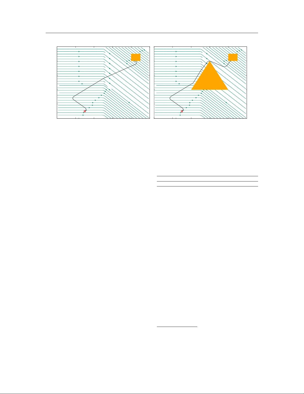
DRAFT : Numer ical Integration and Dynamic Discretization in Heur istic Search Planning o v er Hybrid Domains M iquel R amirez Univ ersity of Melbourne miguel.ramirez@unimelb.edu.au E nrico S cala A ustralian National Univ ersity enrico.scala@anu.edu.au P a trik H aslum A ustralian National Univ ersity patrik.haslum@anu.edu.au S yl vie T hieba ux A ustralian National Univ ersity sylvie.thiebaux@anu.edu.au March 14, 2017 Abstract In this paper we look into the problem of planning over hybrid domains, where change can be both discrete and instantaneous, or continuous over time. In addition, it is requir ed that each state on the trajectory induced by the execution of plans complies with a given set of global constraints. We approach the computation of plans for such domains as the problem of searching over a deterministic state model. In this model, some of the successor states are obtained by solving numerically the so-called initial value problem over a set of ordinary differential equations (ODE) given by the current plan prefix. These equations hold over time intervals whose duration is determined dynamically , according to whether zero crossing events take place for a set of invariant conditions. The resulting planner , FS+, incorporates these features together with effective heuristic guidance. FS+ does not impose any of the syntactic restrictions on process effects often found on the existing literature on Hybrid Planning. A key concept of our approach is that a clear separation is struck between planning and simulation time steps. The former is the time allowed to observe the evolution of a given dynamical system before committing to a future course of action, whilst the later is part of the model of the environment. FS+ is shown to be a robust planner over a diverse set of hybrid domains, taken from the existing literature on hybrid planning and systems. I. I ntrod uction A central research topic in domain– independent automated planning is that of seeking plans o v er hybrid domain de- scriptions that feature both discrete and numeric state v ariables, as w ell as discrete instantaneous and continuous durativ e change via actions and processes ( Fox & Long, 2006). A purely continuous dynamical system is defined by a set differ ential equations ( ode ’s) that specifies ho w the system ev olv es ov er time ( Scheiner man, 2001). Hybrid planning problems correspond to control of switched dynamical systems , which are driv en b y dif- ferent dynamics (set of ode ’s) in different modes . A mode can be defined b y the values of discrete state variables, a region of the continuous state space, or a combination of both ( Goebel, Sanfelice, & T eel, 2009; Ogata, 2010). Planning languages, such as pddl + and our extension of FSTRIPS, model switched dynamical systems compactly in a factored w a y , a v oiding the explicit enumeration of modes. This paper introduces a heuristic search hy- brid planner , FS+ . Like McDer mott’s ( 2003) hybrid planner , OpT op , ours branches ov er the set of applicable instantaneous actions plus a special “waiting” action si m , that simulates continuous state ev olution with the passing of time. The duration of the w aiting action, that discretises time, is not fixed to a single value or a suitably chosen set like in ( Fox, Long, & Magazzeni, 2012), but rather FS+ decides to use a smaller one than the initially set planning 1 T echnical Report - Ramirez M., S cala E., Haslum P ., Thiebaux S. time step, ∆ m a x . The successor state that results from applying the waiting action is the result of simulating system ev olution, according to the dynamics of its current mode, for the dura- tion of the step; computing it is known as the initial value problem in control theory ( Ogata, 2010). For general dynamics there is no analyt- ical solution to this problem, but approximate solutions can be obtained with a v ariety of nu- merical integration methods ( Butcher, 2008). Such methods apply a finer discretisation, us- ing a simulation time step ∆ z . Finally , a v alida- tion step v erifies that the inv ariant condition of the mode ( Ho w ey & Long, 2003) remains true throughout each simulation step. If it does not – which w e refer to as a zero crossing event , follo wing Shin & Da vies ( 2005) – the interval is cut short. Thus, FS+ , in an adaptiv e and to a high degree, unsupervised manner , breaks the time line around specific time points, or happenings ( Fox & Long, 2006), effectiv ely de- termining the right discretisation at each point in the plan on-line. This contrasts with pre- vious work on hybrid planning, which either performs plan v alidation (i.e., checking for zero crossings) off–line ( Ho w ey , Long, & Fox, 2005; DellaPenna, Magazzeni, Mercorio, & Intrig- ila, 2009), or is restricted to specific classes of ode ’s ( Shin & Da vis, 2005; Löhr , Eyerich, Keller , & Nebel, 2012; Coles & Coles, 2014; Bryce, Gao, Musliner , & Goldman, 2015; Cashmore, Fox, Long, & Magazzeni, 2016). A second feature is that FS+ examines modes of the hybrid sys- tem only as they are encountered in the search, in a manner similar to Kuiper ’s ( 1986) qual- itativ e simulation. Since planning languages can compactly express hybrid systems with an exponential number of modes as combinations of processes, it is crucial to a v oid generating or analysing all modes up front ( Löhr et al., 2012). The paper starts b y illustrating a classical problem in control theor y that motivated this research. After that, w e introduce the language supported by FS+ , v ery similar to pddl + , but more succinct, that extends recently revis- ited classical planning languages ( Frances & Geffner, 2015). Then the contributions of this paper are presented. First, w e present the se- mantics of our planning language, that departs from ( Fox & Long, 2006) in some important aspects. S econd, we show how a deterministic state model can account for the semantics giv en for hybrid planning, describing the role pla y ed b y numerical integration and the on–line de- tection of zero crossing ev ents. Third, w e dis- cuss v ery briefly how we integrate two recent heuristics to construct h FS+ , a nov el heuristic, FS+ uses to guide the search for plans. The first of these heuristics is the Interval-Based Relax- ation heuristic for classical numeric and hybrid planning ( Scala, Haslum, Thiebaux, & Ramirez, 2016), the other is the Constraint Relaxed Plan- ning Graph heuristic dev eloped b y ( Frances & Geffner, 2015). Last, w e discuss the perfor- mance of FS+ o v er a diverse set of benchmarks featuring both with linear and non–linear dy- namics, and compare FS+ with hybrid plan- ners that can handle such a div erse range of problems. W e finish discussing the significance of our results and future w ork. II. E xample : Z ermelo ’ s N a viga tion P roblem Zermelo’s navigation problem, proposed by Ernst Zer melo ( 1931), is a classic optimal con- trol problem that deals with a boat navigating on a body of w ater , starting from a point s 0 to end up within a designated goal region s G . While simple, it has a vast number of real- w orld applications, such as planning fuel effi- cient routes for commercial aircraft ( Soler , Oli- v ares, & Staf fetti, 2010). The boat mov es with speed v , its agility is giv en by the turning rate ρ ; both remain constant ov er time. It is desired to reach s G in the least possible time, yet the ship has to negotiate variable wind conditions, giv en by the position dependant drift vector w ( x , y ) = h u ( x , y ) , v ( x , y ) i . States consist of three variables, the current location of the boat ( x , y ) ∈ R 2 and its heading θ 1 . For fixed head- ing θ , w e ha v e that the location of the boat 1 All state variables depend on the time t , that is, are subject to exogenous continuous change ov er variable t , that tracks the passage of time. 2 T echnical Report - Ramirez M., S cala E., Haslum P ., Thiebaux S. Figure 1: T rajectory found by FS+ for two instances of the Zermelo navigation problem with non-homogeneous wind conditions (arrows show wind direction), and non–convex constraints in the instance on the right. The circle denotes the initial state s 0 , the box the set of goal states s G and the triangle is constraint. changes according to the ode : ˙ x = v co s θ + u ( x , y ) (1) ˙ y = v s i n θ + v ( x , y ) (2) The agent can steer the boat to w ards goal states s G s G | = x mi n G ≤ x ≤ x m a x G ∧ y mi n G ≤ y ≤ y m a x G b y altering the angle θ in a suitably defined manner . The function of θ o v er time is in ef fect the control signal ( Ogata, 2010) for this dynam- ical system. In this paper , we account for the range of possible signals by ha ving instanta- neous actions to switch on, off or modulate con- tinuous change ov er certain state variables. In this example, the agent has av ailable three in- stantaneous actions a he ad , po r t , st ar b o ard that account respectiv ely for keeping the boat rud- der steady , push it tow ar ds the right, and to the left. Each of these actions sets an auxil- iary variable ctl to the values straight , left and right . These instantaneous actions cannot be executed in any order , so w e impose a further (logical) restriction by requiring to keep the rudder straight before being able to push it either tow ards the left and the right. These actions account for the possible control switches connecting the set of control modes of a Hybrid A utomata ( Henzinger, 2000). The variable ctl is then used to define the rate of change of θ in the following manner: ˙ θ = − ρ when ctl = left , ˙ θ = ρ when ctl = right , and ˙ θ = 0 other wise. W e note that angles are giv en in radians . On T ime(secs) 0 100 500 600 2030 2130 Action st a r bo ard ah e a d p o rt a he a d s t ar b o a rd ah e a d T able 1: Plan for the left image on Figure 1, reaching goal area in 2, 430 seconds of simulated time, that required 0.32 seconds of real time to be computed. ∆ ma x was set to 100 seconds, and a zero crossing event was detected at t = 2, 030 . the left of Figure 1 w e can see the trajectory fol- lo wing from the plan in T able 1. The rudder is left alone for quite some time, until the boat al- most sails past the goal, and then goes upwind to w ards s G . Global constraints in that scenario require to keep the boat within the bounding box, that coincides with the image extent. On the right in Figure 1 we can see the path that complies with an additional constraint: to stay outside of the golden triangle. III. ∫ - pddl + The planning language w e will use in this w ork, ∫ - pddl + 2 , is the result of integrating Func- tional STRIPS (FSTRIPS) ( Geffner, 2000), and 2 The ∫ in ∫ - pddl + accounts both for the role that the specific integration methods pla y as a implicit part of the modeling and also for the use of functions. The latter follows from the historical fact that in the 16th century , 3 T echnical Report - Ramirez M., S cala E., Haslum P ., Thiebaux S. specific fragments of pddl 2.1 Lev el 2 ( Fox & Long, 2003) and pddl 2.1 Lev el 5 ( Fox & Long, 2006), also kno wn as pddl + . FSTRIPS is a gen- eral modeling language for classical planning based on the fragment of First Order Logic (FOL) inv olving constant , functional and rela- tional symbols (predicates), but no variable symbols, as originally pr oposed by Geffner , and recently augmented with support for quantification and conditional effects (Frances & Geffner, 2016), thus becoming practically equiv alent to the finite–domain fragment of adl ( Pednault, 1986). Its syntax is essen- tially the same as that of the “unofficial” re- vision of pddl , pddl 3.1, first proposed by Helmert ( 2008) as the official pddl variant of the 2008 International Planning Competition, and fully formalised later by Ko v ács ( 2011). T o this we ha v e added support for features pro- posed in pddl 2.1 Lev el 2 ( Fox & Long, 2003) to handle arithmetic expressions, arbitrar y al- gebraic and trigonometric functions ( Scala et al., 2016), and the notion of autonomous pro- cesses in pddl 2.1 Lev el 5 ( Fox & Long, 2006) to account continuous change o v er time. The implementation of ∫ - pddl + is built on top of that in the recent classical planner FS ( Frances & Geffner, 2016). States, preconditions and goals in ∫ - pddl + are described using fluent symbols, whose denotation changes as a result of do- ing actions or the natural effect of processes o v er time. Those symbols whose denotation does not change are fixed symbols and include finite sets of object names, integer and real con- stants, the arithmetic operators ’ + ’, ’ − ’, ’ × ’, ’ ÷ ’, exponentiaton, n–th roots, si n ( ) , co s ( ) and t a n () , as well as the relational symbols ’ = ’, ’ > ’, ’ < ’, ’ ≥ ’ and ’ ≤ ’, all of them following a standard inter pretation. T erms, atoms and for- mulas are defined from constant, function and relation symbols, with both terms and sym- bols being typed . T ypes are given by finite sets of fixed constant symbols 3 . T er ms f ( α ) , where f is a fluent symbol and α is a tuple when calculus was being invented by Newton and Leibniz, written English and Ger man did not differentiate between the sounds for ’s’ and ’f ’. 3 Note that whenev er w e use the term “real numbers” of fixed constant symbols, are called state vari- ables , and states are determined b y their val- ues. Primitiv e Numeric Expressions ( PNE ) ( Fox & Long, 2003) correspond exactly with w ell formed arithmetic terms combining constants, state variables, arithmetic operators and other functions. Instantaneous actions a and processes p are described by the type of their arguments and tw o sets, the (pre)condition and the ef fects. Ac- tion a ’s preconditions Pr e ( a ) and process p ’s conditions K ( p ) are both formulae. Actions and processes differ in the definition of their effects. Action a effects update instantly the de- notation of state v ariables f ( α ) as a result of ap- plying a . Process p effects describe ho w the de- notation of state v ariables f ( α ) changes as time goes by . State v ariables f ( α ) that appear only in the left hand side of action effects are effec- tiv ely inertial fluents ( Gelfond & Lifschitz, 1998). On the other hand, those v ariables f ( α ) ap- pearing on the left hand side of process effects, and possibly as well in the effects of instanta- neous actions, are non–inertial ( Giunchiglia & Lifschitz, 1998) as their denotation can change ev en when left alone. Formally , the effect of an action a is a set of updates of the form g ( β ) : = ξ a , where g ( β ) and ξ a are ter ms of the same type, expressing how g ( β ) changes when a is taken. The effects of a process p is also a set of update rules, but process updates, instead of an assignment, are ode ’s ˙ f ( α ) = ξ p 4 . The value of a time-dependent state variable f ( α ) after t 0 − t 0 time units, pro vided that p is the only process affecting f ( α ) as prescribed b y the update rule ˙ f ( α ) = ξ p , is giv en by the follo wing integral equation f 0 ( α ) = f 0 ( α ) + Z t 0 t 0 ξ p ∂ t (3) where t 0 > t 0 is a positiv e finite number , f 0 ( α ) 5 w e actually refer to the finite set of rational numbers that can be represented with the finite precision arithmetic sup- ported in most general–pur pose programming languages. Similarly for “integers”. 4 ˙ f ( α ) denotes the deriv ativ e of f ( α ) o v er time. 5 W e decouple v ariable symbols from time t following the notation typical from contemporar y manuals on ode ’s and numerical analysis e.g. Butcher ’s (2008) . 4 T echnical Report - Ramirez M., S cala E., Haslum P ., Thiebaux S. is the v alue of state v ariable f ( α ) at time t 0 , and t 0 is the time associated with the initial conditions f 0 ( α ) . The type allow ed for f ( α ) and ξ p is restricted to be the real numbers. W e im- pose a further restriction on ξ p , namely that it needs to be an integrable function in the interv al [ t 0 , t 0 ] , so the rightmost term in Equation 3 is finite . Global (state) constraints C ( Lin & Reiter, 1994) allow to describe compactly restrictions on the v alues that state v ariables f ( α ) can take o v er time. FS+ currently supports global con- straints C giv en as CNF for mulae, where each clause ϕ is a disjunction of relational formu- lae. This allows us to model state constraints similar to those proposed ( 2014). Since ∫ - pddl + supports disjunctiv e formulae, by exten- sion it accounts for implication as required by Iv anko vic’s switched constraints P ⊃ S , where P is a conjunction of literals of so–called primary v ariables, equiv alent to our state v ariables f ( α ) , and S is an arbitrary formula o v er so–called secondary v ariables. How ev er ∫ - pddl + cannot represent the latter , as their denotation in any giv en state is not fixed, as their v alue is giv en b y those featured in the models (satisfying as- signments ov er S ) of the constraints. Last, the planning tasks we consider are tu- ples P = h F , I , O , P , G , C i where I and G are the initial state and goal formula, O is a set of instantaneous actions, P is a set of processes, C is a set of state constraints and F describes the fluent symbols and their types. I must define a unique denotation for each of the symbols in F , and satisfy ev ery C ∈ C . IV . S emantics of ∫ - pddl + W e first briefly revie w the semantics of FSTRIPS, following Francès and Geffner ( 2015, 2016). Then we discuss continuous change on state variables as the timeline is broken into a finite set of inter v als, each with an associated set of active processes ( Fox & Long, 2006), or mode (Ogata, 2010). The logical inter pretation of a state s is de- scribed as follows in a bottom–up fashion. The denotation of a symbol or term φ in the state s is written as [ φ ] s . The denotation of objects or constants symbols r , is fixed and independent from s . Objects o denote themselv es and the denotation of constants (e.g. 3.14) is giv en b y the underlying programming language 6 . The denotation of fixed (typed) function and rela- tional symbols can be pro vided extensionally , b y enumeration in I , or intensionally , by attaching external procedures ( Dornhege et al., 2012) 7 . The dynamic part of states s is represented as the value of a finite set of state variables f ( α ) . From the fixed denotation of constant symbols and the changing denotation of fluent symbols f captured b y the values [ f ( α ) ] s , the denota- tion of arbitrary terms, atoms and for mulas follo ws in a standard w a y . An instantaneous action a is deemed applicable in a state s when [ P re ( a ) ] s = > , and the state s a resulting from applying a to s is such that, 1) all state con- straints are satisfied, [ C ] s a = > for ev er y state constraint C ∈ C , and 2) [ g ( β ) ] s a = [ ξ a ] s for ev er y update g ( β ) : = ξ a triggered by a , and [ f ( α ) ] s a = [ f ( α ) ] s otherwise. A sequence of in- stantaneous actions ac t = ( a 1 , . . . , a j , . . . , a n ) , a j ∈ O , is applicable in a state s when [ P re ( a 1 )] s = > , and for ev er y inter mediate state s a j , j > 1, resulting from applying action a j − 1 in s a j − 1 , it also holds that [ P re ( a j )] s a j . W e write s [ ac t ] for the state resulting from applying sequence ac t on state s . Because our time domain, R + 0 , is dense, the number of states is infinite. W e introduce structure into this line b y borrowing Fox & Long’s ( 2006) notion of happenings η , distin- guished points on the time line where an event takes place or an instantaneous action is exe- cuted. In betw een each pair of happenings is a steady interval during which the state ev olv es continuously according to the set of activ e pro- cesses, or modes, that characterize a dynamical system. W e require happenings to exist at any point where processes start or end, thus en- suring the set of active processes is constant 6 In our case, C++. 7 Arithmetic, algebraic and relational symbols are repre- sented intensionally when the types of state variables and constants present in an arithmetic term are the “integers” or the “reals”. 5 T echnical Report - Ramirez M., S cala E., Haslum P ., Thiebaux S. throughout each inter v al. Formally , a happening η is characterised b y its timing , T ( η ) , mapping η to t ∈ R + 0 , the state s ( η ) at that time, and a sequence ac t ( η ) of instantaneous actions applied at the happening. Note that s ( η ) is the state be- fore ac t ( η ) is applied. An interval is char - acterised by the two happenings that mark its start and end: H i = h η − i , η + i i , where the end happening has no associated actions, i.e., ac t ( η + i ) = h i . The duration of H i is the dif- ference ∆ i = T ( η + i ) − T ( η − i ) and w e assume a finite upper and low er bounds on the dura- tion of each interval, i.e., ∆ mi n ≤ ∆ i ≤ ∆ m a x , are pro vided as part of the problem descrip- tion. The low er bound ∆ mi n can indeed be set to 0, but in that case w e observe that in- troduces the possibility of plans with infinite length, their execution being referred to as a Zeno’ s execution in existing literature in hybrid control theory ( Goebel et al., 2009). The v al- ues of state variables f ( α ) at the start of the interval H i are given by the state s i 0 that results from applying the sequence of actions ac t ( η − i ) associated with the start happening to the state s ( η − i ) , i.e. s i 0 ≡ s ( η − i )[ ac t ( η − i )] . During the interval H i , continuous state v ariables may be affected b y the set of processes that are active in H i . The state at the end of H i , s ( η + i ) , is defined by integrating the activ e processes’ ef- fects, following the general form of Equation 3. W e define the set of activ e processes µ i ⊆ P , or mode , associated with interval H i , as those whose conditions hold in the state at the inter- v al’s beginning: µ i = { p | p ∈ P , s i 0 | = K ( p ) } W e note that h s i 0 , µ i i is the dynamical system associated to H i . S ev eral active processes can affect the same state v ariable f ( α ) . Recall that process effects specify the rate of change: w e follo w the standard convention that process effects superimpose, by adding together the rates of change of all activ e processes affecting f ( α ) ( Ogata, 2010). The v alue of state v ariable f ( α ) in state s ( η + i ) is then giv en b y [ f ( α ) ] s ( η + i ) = [ f ( α ) ] s i 0 + Z T ( η + i ) T ( η − i ) ∑ p ∈ R f ( α ) δ i p ξ p ∂ t (4) where R f ( α ) ⊆ P is the set of pr ocesses p where f ( α ) appears on the left hand side of some ef- fect ξ p , and the activation variable , δ i p , for each process p is the characteristic function of the mode µ i , meaning that δ i p = 1 if p ∈ µ i and 0 otherwise. Equation 4 can be simplified. First, note that as long as µ i remains stable , that is, the set of activ e processes does not change ov er the duration of interval H i , δ i p does not de- pend on time t . S econd, the restriction on ξ p imposed in the previous S ection, i.e. that ξ p is a continuous function o v er [ T ( η − i ) , T ( η + i )] , enables the direct application of Fubini’s The- orem ( 1907). Pro vided that µ i is stable w e can rewrite Equation 4 as [ f ( α ) ] s ( η + i ) = [ f ( α ) ] s i 0 + ∑ p ∈ R f ( α ) ∩ µ i Z T ( η + i ) T ( η − i ) ξ p ∂ t (5) Next, w e define a condition that implies the in- terval H i is stable, i.e., that µ i does not change during H i . T o do this, w e v erify that none of the following happens at any point t ∈ [ T ( η − i ) , T ( η + i )] : (1) the truth of the conditions K ( p ) of some process p ∈ P changes, (2) some state constraint C ∈ C is violated, and (3) w e do not “shoot through” sets of states where the goal G is true. The absence of each of these ev ents can be expressed as a condition, the conjunction of these three conditions is the invariant for mula I ( H i ) : ¬ G ∧ ^ p ∈ µ i K ( p ) ∧ ^ p 0 ∈ P \ µ i ¬ K ( p 0 ) ∧ ^ C ∈C C (6) ( Ho w ey & Long, 2003; How ey et al., 2005). If the invariant I ( H i ) holds throughout H i , then H i is stable. Note that sub-formulae of I ( H i ) that mention only state variables f ( α ) not af- fected by any process alw a ys remain true ov er H i . Following Shin & Da vies’ ( 2005), w e refer to a change in the truth v alue of I ( H i ) as a zero crossing event . 6 T echnical Report - Ramirez M., S cala E., Haslum P ., Thiebaux S. Definition 1. (Zero Crossing Ev ent) Let H i be a inter v al with timings T ( η − i ) and T ( η + i ) , and inv ariant I ( H i ) . A zero crossing event occurs whenev er for some t 0 s.t. T ( η − i ) < t 0 < T ( η + i ) , I ( H i ) is false . Definition 2. (Steady Inter v als) Let H i be a interval with timings T ( η − i ) and T ( η + i ) , state s i 0 and mode µ i . Whenev er zero crossing ev ent occurs for some t 0 s.t. T ( η − i ) < t 0 < T ( η + i ) , then the inter v al H i is a steady interval , whose dynamics are fully described by the dynamical system h s i 0 , µ i i . W e are no w ready to define what is a solu- tion for our planning tasks. A valid plan π for hybrid planning task P is a finite sequence π = ( H 0 , H 1 , . . . , H i , . . . , H m ) of steady inter vals H i , such that (1) s ( η + m ) | = G , and (2) T ( η − m ) = T ( η + i − 1 ) . The optimality of plans depends on the metric the modeller speci- fies for P as ev aluated on s ( η + m ) : our extended FSTRIPS language, like pddl 3.1, enables the modeller to specify both obvious metrics such as the ov erall duration of π (i.e. ∑ ∆ i ) and more intricate ones as needed. i. Comparison with pddl + The planning language we define is very sim- ilar to, and certainly ow es many of its core concepts to, the specification of pddl + giv en b y Fox & Long ( 2006). How ev er , it separates in tw o wa ys, in the inter pretation of plans and not accounting for the pddl + notion of events completely . First, w e consider only the computation of plans with finite duration and representation, consisting of a finite but unbounded number of happenings. Our interpretation of happenings is that they break the continuous timeline into a finite sequence of inter vals during which the continuous effects on state variables are station- ary . The number of states in each interval is infinite, but all such inter mediate states are cat- aloged implicitly b y the states at the happenings that mark the extent of the inter v al ( Pednault, 1986). Second, w e allow the planner to execute a fi- nite but unbounded sequence of instantaneous actions at a happening η without any restric- tion, such as commutativity , on their effects. This allows us to model, for instance, the net- w ork of v alv es in the rocket engine discussed in the classic w ork of W illiams & Nay ak ( 1996) without an explosion in the number of instanta- neous actions required to represent all possible combinations of v alv e positions. In contrast, pddl + mandates a non-zero time separation (kno wn as the “ e ”) betw een non-commutativ e instantaneous actions. This restriction is moti- v ated by the assumption that actions, although modelled as instantaneous, cannot actually be executed in zero time ( Fox & Long, 2006). Ho w- ev er , for those cases in which a temporal sepa- ration, or “cool do wn” period, betw een actions is motivated by the application domain, this can be modelled (using an auxiliar y process representing a timer , for instance) also in our setting. Thus, no expressivity is lost when it comes to model limitations in the execution of plans. Finally pddl + considers events to be “first– class citizens” in the language, with seman- tics best described as “exogenous” instanta- neous actions, rather than implicitly defined as points where invariant conditions change. Although ev ents are in some cases a natu- ral and conv enient modeling device, some of their effects can also be captured by introduc- ing suitably defined global constraints or com- piled into process preconditions. For instance in the M ars S olar R over domain proposed b y ( 2005), one can do a w ay with the ev ents sunset and sunrise b y ha ving a global timer for the whole day , and modifying accordingly the preconditions of the processes day time and night time . This also a v oids some of the problems Fox et al observe to be associated with plan validation in the presence of ev ents. On the other hand, uses of ev ents to model spontaneous changes in the dynamics, are not accounted for . A natural and familiar example of such phenomena is that of ellastic collisions betw een bodies with the same mass, where the direction of acceleration changes as conse- 7 T echnical Report - Ramirez M., S cala E., Haslum P ., Thiebaux S. quence of the collision. Accounting for these w ould be necessar y to model accurately as a hybrid domain real-w orld tasks such as pla y- ing solitaire pool. V . B ranching and C omputing S uccessor S t ates As outlined in the Introduction, FS+ searches for plans π of hybrid planning task P via for- w ard search ov er a deter ministic state model M ( P ) = h S , s I , A 0 , S G , A p p , f i where each element is defined as follo ws. The state space S is given by all the possible combinations of denotations for fluents F plus an auxiliary state v ariable t ( ) to represent the location of states s on the time line. Actions A 0 = O ∪ { s i m } include the instantaneous actions O in P and a si m action that updates t ( ) and simulates the w orld dynamics as giv en b y the continuous effects of processes P . Goal states S G ⊆ S are those states s s.t. [ G ] s = > ; s I is like I .The applicability function A p p corresponds exactly with the notion of applicable actions discussed in the previous Section, while si m actions can be applied in ev er y state s ∈ S . f ( a , s ) = s a for instantaneous actions a ; w e dev ote the rest of this S ection to define f ( si m , s ) . S olutions to M ( P ) are paths π 0 = ( a 0 , . . . , a n ) connecting s I with some s ∈ S G . The plan π made up of intervals H j is obtained from paths π 0 b y ob- serving that (1) for ev ery action a j = si m action in π 0 , there is an inter v al H j in π , (2) the timing of happening η − j is [ t ( ) ] s l , where s l = s 0 or s l = f ( a l , s l − 1 ) , a l ∈ π 0 a l = si m , l < j , (3) the tim- ing of happening η + j is [ t ( ) ] s j , s j = f ( s j − 1 , si m ) , and (4) ac t ( η − j ) ⊂ π 0 , defined as ac t ( η − j ) = ( a k , . . . , a j − 1 ) , k = 0 or a k − 1 = s i m . As suggested b y this mapping of paths betw een initial and goal states in M ( P ) into sequences of intervals H i , the action si m (1) pr edicts successor states b y solving Equation 5 for ev ery state variable f ( α ) appearing on the left–hand side of effects of processes p ∈ µ i , and (2) validates the as- sumption that µ i is stable checking whether for some t zc in the inter v al [ T ( η − i ) , T ( η − i ) + ∆ m a x ] the truth of I ( H i ) changes. When that is the case, auxiliary v ariable t ( ) is set to t zc instead of T ( η − i ) + ∆ m a x , in turn setting T ( η + i ) to t zc as w ell. W e note that both of these problems can- not be solv ed exactly in general, as both state prediction, or general symbolic integra- tion, and v alidation, or finding roots of real– v alued functions ( Ho w ey & Long, 2003), can be shown to be undecidable b y Richardson’s Theorem ( 1968). Consequently , it will nev er be possible to guarantee that plans are v alid, but that is not necessar y to compute plans that are accurate enough to infor m the solution of real-w orld engineering problems. While exact, general solutions are out of reach, w e can tur n to numerical approximation methods for both prediction and validation. W e discuss ho w w e approximate the prediction of successor states and their validation next. i. Related W ork: Analytical S olutions and Linear Dynamics The implications of Richardson’s Theorem on the validity of plans are indeed quite negativ e, and it has motiv ated the planning community to look into less expressiv e, y et still pow erful and widely applicable, fragments of hybrid planning, where the for m of processes effects is restricted in some w a y . W e dev ote this S ection to briefly discuss existing w ork on a fragment that, while still undecidable, does not require to explicitly discretise time. A substantial part of the existing literature on hybrid planning studies domains where the right–hand side ξ p of processes p in modes µ i reachable from the initial state, and hence the dynamical systems associated with such modes h s i 0 , µ i i , has a specific for m: that of general linear expressions, ξ p : b p + ∑ f ( α ) ∈ F w p f ( α ) f ( α ) (7) In that case, the combined effects of processes in µ i can be written compactly in matrix for m as follows: ˙ x = A x + b (8) 8 T echnical Report - Ramirez M., S cala E., Haslum P ., Thiebaux S. where x is made of (time–v arying) state vari- ables f ( α ) and both A and b follo w fr om the coefficients in Equation 7. The dynami- cal systems Equation 8 accounts for are a use- ful and w ell known class of dynamical sys- tems, known as Linear T ime–Invariant (L TI) systems ( Scheiner man, 2001; Ogata, 2010), for which there exists an analytical solution to Equa- tion 8. L TI systems are good models for a huge range of domains ( Löhr et al., 2012), yet still lack generality since linear approximations of physical processes are not alw a ys reasonable. From a practical standpoint, solving the initial v alue problem amounts to computing the expo- nential of matrix A . Matrix exponentiation is a non–trivial linear algebra problem ( Horn & Johnson, 2013), that needs to be solv ed for every possible system h s i 0 , µ i i . Existing approaches rely on precomputing the closed form for Equa- tion 8, something which is tricky in domains like McDermott’s C onvoys ( 2003) where enu- meration can be impractical. ii. T o Successor States via Numerical Integration Computing the state corresponding to the hap- pening η + i requires si m to solv e the initial value problem ( Butcher, 2008), for the dynamical system h s i 0 , µ i i associated with the inter val H i . FS+ does so relying on numerical integration methods ( Butcher, 2008) that do not require syntactic restrictions on the effects ξ p of pro- cesses p ∈ P in order to be applicable. This generality comes at a cost: since numerical integration relies on discretization of the free v ariable, time t in this case, and w e need to introduce a new parameter , ∆ z , the simulation step . The computation of the state s ( η + i ) for a giv en inter v al H i , proceeds as follows. W e start observing that giv en any happening η , a mode µ i and the state s ( η ) , the state s ( η 0 ) of another happening η 0 s.t. T ( η 0 ) = T ( η ) + ∆ z is defined as s ( η 0 ) = Φ [ s ( η ) , µ i , ∆ z ] where Φ [ · ] is the specific numerical integration method being used to predict the values of state v ariables f ( α ) being changed b y processes p ∈ µ i . Computing the state s ( η + i ) amounts to integrate Equation 5 o v er inter vals of duration ∆ z , and repeat this k times where k = $ T ( η + i ) − T ( η − i ) ∆ z % Whenev er k ∆ z < ∆ i an additional call to the integration method Φ [ · ] using ∆ z 0 as the simu- lation step is needed and ∆ z 0 = T ( η + i ) − ( T ( η − i ) + k ∆ z ) The simplest integrator Φ [ · ] implemented in FS+ is the Explicit Euler Method ( Butcher, 2008), that deter mines the v alues of f ( α ) in state s k follo wing Equation [ f ( α ) ] s ( η 0 ) = [ f ( α ) ] s ( η ) + ∆ z ∑ p ∈ µ i [ ξ p ] s ( η ) (9) which is the recurr ence relation for integral Equa- tion 5. The conv ergence of numerical inte- gration methods like the one in Equation 9 is v er y sensitive to the choice of ∆ z , and for non– linear ξ p these methods can be easily shown to div erge ev en for small v alues of ∆ z . On the other hand, more robust numerical integra- tion methods, such as the Runge–Kutta integra- tors ( Butcher, 2008), are significantly mor e com- plicated than Equation 9 y et still much cheaper than matrix exponentiation. Amongst these, FS+ currently implements the midpoint rule , the 2nd order Runge–Kutta integrator that Butcher refers to as R K 22. FS+ also implements the iterative or multi–step Implicit Euler method [ f ( α ) ] s j + 1 ( η 0 ) = [ f ( α ) ] s ( η ) + ∆ z ∑ p ∈ µ i [ ξ p ] s j ( η 0 ) (10) where [ f ( α ) ] s 0 ( η 0 ) is given b y Equation 9, and iteration continues until the following fixed– point is reached: | [ f ( α ) ] s ( η 0 ) j + 1 − [ ξ p ] s ( η 0 ) j | < e (11) Last, for problems where all process effects are linear expressions, w e note that the “messy” numerical integrator Φ [ · ] currently a v ailable in FS+ could be readily substituted with the 9 T echnical Report - Ramirez M., S cala E., Haslum P ., Thiebaux S. analytical solution of the L TI system giv en b y µ i , calling an external solv er online instead of doing so as pre–processing step, during the search. Such a change w ould entail significant gains in precision, but w e suspect the cost of computing the analytical solution w ould ha v e a significant negative effect on run–times. iii. T esting for Zero Crossings The inv ariant I ( H i ) is a conjunction of parts, each of which can be e v aluated separately . Some parts may be disjunctiv e (thus non- conv ex) as a result of negating conjunctiv e goals G or process conditions K ( p ) ( Ho w ey & Long, 2003), or from disjunctive global con- straints. Recall, ho w ev er , that the main aim of validation is to pro v e the absence of a zero- crossing ev ent in the simulated time interval. This allows us to simplify the problem by test- ing necessary conditions for a zer o-crossing ev ent to occur; if those are not satisfied, w e can con- clude no such ev ent happened, and hence that the inter v al is steady . If a zero-cr ossing ev ent ma y ha v e occured, it is sufficient to find an time point t in the inter val such that the ev ent is necessarily after t . The length of the steady interval is then shortened, and the planner in- serts a new happening at t from which it can branch. T o validate a disjunctiv e formula ϕ = φ 1 ∨ . . . ∨ φ l o v er an inter v al starting from state s , w e test instead ϕ s = V j s.t. s | = φ j φ j , that is, the conjunction of the disjuncts that are true in s , since the falsification of at least one of those disjuncts is a necessary condition for ϕ to be- come false. After strengthening I ( H i ) in this fashion, we introduce k happenings η j i with timings T ( η j i ) = T ( η − i ) + j ∆ z , and T ( η − i ) + k ∆ z < T ( η + i ) , and states resulting from calls to an integrator Φ [ · ] using a finer grained sim- ulation step ∆ h 8 . Where ξ l , ξ r are arithmetic terms and ⊕ is a relational symbol, the truth of an atomic for mula ψ = ξ l ⊕ ξ r , in state s is tied to the sign of the function f ψ f ψ ( s ) = [ ξ l − ξ r ] s (12) 8 ∆ h is set somewhat arbitrarily to 0.1 ∆ z . – ψ can only change from true to false if f ψ ( s ) changes sign. Whether this occurs in the in- terval betw een tw o consecutiv e happenings η j i , η j + 1 i can be deter mined by direct application of the following classical result from mathemati- cal analysis: Theorem 3. (Intermediate V alue Theorem) Let f be continuous on the closed interval [ a , b ] . If f ( a ) ≤ y ≤ f ( b ) or f ( b ) ≤ y ≤ f ( a ) then there exists point c such that a ≤ c ≤ b and f ( c ) = y. W e observ e that (1) f ψ is a continuous func- tion, following from the constraint on effects of processes ξ p to be integrable , and (2) if f ψ ( η j i ) < 0 ( > 0) and f ψ ( η j + 1 i ) > 0 ( < 0), then there necessarily exists a happening η zc , T ( η zc ) ∈ [ T ( η j i ) , T ( η j + 1 i )] such that f ψ ( η zc ) = 0, i.e. a zero–crossing ev ent for ψ takes place at time T ( η zc ) . The earlier strengthening of disjunctions implies that ϕ s is falsified as soon as this happens for any atomic for mula ψ is. In this case, the interval H i is shortened by setting η + i = η j i . The treatment of disjunctiv e inv ariants means that happenings ma y be inserted where not truly needed, since a disjunction can re- main true ev en if one of its disjuncts is falsified. This may lead to a deeper search than neces- sary , but any path found will still be v alid. If the dynamics in the interval oscillate rapidly , the indicator function f ψ ma y change sign sev- eral times within the validation time step ∆ h ; thus, the procedure ma y also fail to detect a zero-crossing ev ent. As noted earlier , this is an una v oidable consequence of the undecidability of the root-finding problem in general. VI. S earching for P lans In the previous Section we ha v e mapped our take on planning ov er hybrid systems into the problem of finding a path in a deter min- istic state model M ( P ) . This enables us to use, off–the–shelf without modifications, any kno wn blind or heuristic sear ch algorithm, such as Breadth–First S earch or Greedy Best First S earch, to seek plans. Still, heuristic 10 T echnical Report - Ramirez M., S cala E., Haslum P ., Thiebaux S. guidance is essential for scaling up ov er these domains: none of the instances discussed in the next S ection are solvable b y Breadth–First Search when doing on–line validation of suc- cessor states. In order to obtain a heuristic, FS+ follo ws Scala et al. ( 2016), and compiles a w ay processes p as instantaneous actions a p . That is, for each update rule ˙ f ( α ) : = ξ p w e introduce an action effect that mimicks Equa- tion 9 f ( α ) : = f ( α ) + ∆ m a x ξ p (13) where ∆ m a x is the planning step. Then, on the resulting classical planning task P nu m , which is like P but with P = ∅ , w e apply a nov el heuristic, h FS+ , that integrates tw o recent w orks. One is the A ibr relaxation ( Scala et al., 2016) that generalizes the notion of value– accumulation semantics ( Gregory , Long, Fox, & Beck, 2012) to dense intervals defined ov er nu- meric variables. The other is the C rpg heuristic b y Francès and Geffner ( 2015), dev eloped to ex- ploit the structure of planning tasks exposed b y FSTRIPS. h FS+ extends the constraint language supported b y C rpg to support real–v alued v ari- ables, defined ov er intensionally represented domains, i.e. intervals instead of sets. S cala et al ’s convex union operator is then used to succinctly accumulate the intervals revised af- ter applying actions on each lay er of the C rpg , thus propagating upper and lower bounds ov er numeric variables along with atomic for mulae across la y ers. h FS+ estimate corresponds to the number of actions and processes that are needed to get into a lay er of the C rpg where the goal is satisfied. FS+ relies on the C p frame- w ork G e C ode 9 as the latest versions of Francès and Geffner (2016) planners do. VII. E xperiment al E v alu a tion In order to evaluate FS+ w e ha v e selected a number of benchmarks already proposed in the literature on hybrid and numeric planning, as w ell as the Zermelo’s navigation problem (Z ermelo ) discussed in S ection II. The crite- rion used to select benchmarks was first and 9 V ersion 5.0.0 av ailable at http://www.gecode.org/ foremost to consider a div erse representation of the kind of linear and non–linear that can be modeled with ∫ - pddl + , and pddl + , with non–trivial branching factor . T able 2 lists the domains considered, along with the pointers to the publication describing them and a clas- sification of their dynamics. Benchmarks are considered to ha v e linear dynamics (L) when ev- ery reachable h s i 0 , µ i i is a L TI system. T wo spe- cial cases of L TI systems ( Scheiner man, 2001) are considered, namely , homogenous (H) sys- tems, where b = 0 , and non–homogenous (NH) systems, where A = 0 . C onvoys and N on L inear C ar instances wer e taken from ( Scala et al., 2016). For two of the domains, namely A gile R obot and O rbit al R endezvous , no pddl + formulation was a vailable for us to use, so we coded them up from scratch fol- lo wing Löhr ’s description in his PhD disserta- tion (2014). W e next briefly discuss some interesting fea- tures of the domains and how ev ents and du- rativ e actions w ere handled when present in existing pddl + for mulations. In McDer mott’s C onvoys the number of possible modes is giv en by the possible combinations of assign- ments of convo ys and point-to-point routes in the na vigation graph. This potential combina- torial explosion was something intended, as McDermott’s points in his paper ( 2003). O r - bit al R endezvous required us to compile a w ay the durative actions present in Löhr ’s model follo wing the discussion in S ection 4 of Fox & Long paper on pddl + ( 2006), but instead of introducing a “stop“ action, w e introduce an auxiliary “timer ” variable set b y the “start” ac- tion, whose value decreases as an effect of the process being triggered. Besides Löhr ’s fiv e hand crafted instances, w e ha v e generated a number of random ones, following a Gaussian distribution around the initial states featured in Löhr ’s instances. W e report the results of the planners on each set to show the robustness of the planners when slight perturbations are introduced in initial states. Last, the instances of A gile R obot w e consider hav e no obstacles, but do ha v e dead–ends: when (if) the robot v e- locity reaches the v alue of 0, there is no wa y to 11 T echnical Report - Ramirez M., S cala E., Haslum P ., Thiebaux S. Domain P & G Dyn Source A gile R obot L L, H (Löhr, 2014) O rbit al R endezvous L L, G (Löhr, 2014) C onvoys L L,NH (McDer mott, 2003) I ntercept NL L, NH (Scala et al., 2016) Z ermelo L NL (Zermelo, 1931) 1D P owered D escent L L, G (2016) N on L inear C ar L NL (Bryce et al., 2015) D ino ’ s C ar L NL (Piotrowski et al., 2016) T able 2: T axonomy of domains according to expressions, in preconditions, process conditions, goals (P & G) and process effects (Dyn), being linear (L) or non–linear (NL) . We further distinguish three different sub-clases for Linear dynamics: general (G), homogenous (H), non–homogeneous (NH). See text for details. put it back into motion. Ev ents in the domains P owered D escent and D ino ’ s C ar w ere used to introduce dead end states when the trajecto- ries induced by plans hit a region of the state space where a giv en property φ holds. W e translated these directly as global constraints ¬ φ , doing a wa y with no longer necessary aux- iliary predicates present in Piotro wski’s model that enable actions and processes. Conv ersely , global constraints ψ in Z ermelo , A gile R obot , O rbit al R endezvous and N on L inear C ar w ere translated into ev ents with precondition ¬ ψ and effects that delete irrev ocably auxiliar y predicates in the preconditions of actions and processes. FSTRIPS and pddl + domains and sample instances 10 . W e ha v e compared FS+ with four state–of– the–art hybrid planners, UPMurphi ( DellaPenna et al., 2009), DiNo ( Piotro wski et al., 2016), ENHSP ( Scala et al., 2016) 11 and SMTP lan + ( Cashmore et al., 2016). T able 3 shows co v er - age and run times for the three first planners. W e hav e only managed to run SMTP lan + on I ntercept , where it solv ed all the instances in less than a second. Its authors reported, via personal communication, that dynamics other than non–homogenous linear ( N H ) are not sup- ported at the time of writing this. In C on - voys SMTP lan + failed to generate a for mula. W e used the planning step ∆ m a x as the dis- cretization parameter for UPMurphi DiNo and ENHSP . The v alues for ∆ m a x follo w either from 10 A v ailable from the authors after request. 11 In ev ery case, w e use the latest version av ailable from the author ’s website. the v alues used in the papers discussing each domain, in the case of Z ermelo w e perfor med an analysis similar to the one perfior med by Pi- otro wski’s for P owered D escent ( 2016). In ad- dition, DiNo requires bounds on plan duration to be supplied as a parameter for its heuristic estimator . W e used the v alues given b y Pi- otro wski et al when av ailable, other wise w e used the duration obtained by the FS+ planner . W e sho w in T able 3 tw o of out of six configura- tions of FS+ tested, where we considered each of the three integration methods implemented, turning on and off the testing for zero cross- ings. The tw o configurations chosen show ed the best trade–off betw een run times, cov er- age and plan duration over these benchmarks . In all cases we used a generic implementation of Greedy Best First Search. T able 3 sho ws that the tw o best perfor ming FS+ configurations clearly dominate UPMurphi and DiNo on ev ery domain but P owered D e - scent . W e consider this results to be indicative , w e ha v e obser v ed the perfor mance of UPMurphi and DiNo to be v ery sensitiv e to the parame- ters used to discretise time and any numeric variables . Compared with ENHSP , w e can see that by doing considerably more computation while searching for plans, the FS+ planners ha v e similar or superior runtimes and co v er - ages across all the domains considered. Also, FS+ plans reach goal states faster when on– line zero crossing detection is enabled. This pro vides evidence that the numerical integra- tion and on–line discretization mechanisms proposed in this planner can pa y of f ov er a 12 T echnical Report - Ramirez M., S cala E., Haslum P ., Thiebaux S. UPMurphi DiNo ENHSP FS+ RK 22, N V FS+ RK 22 Domain ∆ ma x I S R D S R D S R D S R D S R D A gile R obot 0.5 100 82 1.11 14.46 82 21.10 18.68 100 10.55 8.5 100 0.47 7.0 100 8.00 6.5 1.0 100 0 n/a n/a 0 n/a n/a 0 n/a n/a 100 0.14 10.0 97 0.89 7.4 C onvoys 1 6 2 2.58 18.50 3 99.31 15.33 6 4.21 11.7 6 3.57 12.3 6 4.78 11.6 D ino C ar 1 10 10 1.78 15.00 10 176.00 16.80 10 0.07 12.0 10 0.01 11.0 10 0.03 11.0 I ntercept 0.1 10 12 204.16 62.17 0 n/a n/a 10 5.68 10.6 8 39.00 10.3 10 28.28 10.4 1 10 0 n/a n/a 0 n/a n/a 0 n/a n/a 0 n/a n/a 10 85.93 10.5 N on L inear C ar 1 8 10 1.78 15.00 10 176.00 16.80 8 0.55 10.4 8 1.68 10.5 8 0.72 10.2 O rb . R end . (L öhr ) 100 5 1 35.92 9900 0 n/a n/a 5 0.36 2300.0 5 0.26 2900.0 5 0.46 2223.4 (R andom ) 100 100 1 34.20 2100 0 n/a n/a 100 0.31 2104.0 100 0.09 2534.0 100 0.34 2059.8 P owered D escent 1 20 10 209.64 26.10 18 47.25 40.33 20 1.99 31.4 19 2.75 31.1 16 1.80 28.5 Z ermelo 100 100 0 n/a n/a 0 n/a n/a 92 6.16 2284.8 98 1.04 2225.5 94 1.23 2098.9 T able 3: Coverage of UPMurphi , DiNo , ENHSP and FS+ over the domains in T able 2. T imeout (TO) was set to 1, 800 seconds and physical memory limited to 4 GBytes. ∆ ma x is the planning time step used, I is the number of instances for each domain, S is the number of instances solved by the planner , R is the average run-time (in seconds) and D is the average duration of the plans in seconds for all the domains but C onvoys , where it is given in hours. UPMurphi , DiNo and ENHSP all use ∆ ma x as their discretisation step. T wo variants of FS+ are considered, FS+ RK 22 uses the RK 22 integrator checking for zero crossings of Equation 6, FS+ RK 22, N V uses the same integrator but does not check for zero crossings. ∆ z is set to 0.1 ∆ ma x for the FS+ planners. NS indicates that the planner did not support the domain, “Crashes” that the planner crashed during execution. broad c lass of domains. W e also note that the FS+ planners can solv e the same domains b y increasing ∆ m a x , doing less w ork to find better plans in A gile R obot , but in three instances where our dynamic discretization strategy re- sults in very deep searches, and solving all in- stances of I ntercept . Somewhat surprisingly , FS+ RK 22 solv es less problems than FS+ RK 22, N V in A gile R obot , when ∆ m a x = 1. T esting for zero crossings not only av oids generating un- sound plans, sometimes resulting on the search abandoning a v ery deep plan prefix, in which case FS+ RK 22 finds few er plans as it times out. On other occasions, it does create opportuni- ties to reach a goal state by interrupting an interval H i , bringing about shallow er searches, in which case FS+ RK 22 finds more plans. The latter follows from considering zero crossings for the goal formula in Equation 6 and prev ent- ing the planner from ov ershooting and ruling out plan prefixes which result in “orbiting” the goal region. The most dramatic impact of this observation becomes apparent in the I nter - cept when ∆ m a x is 1. W e consider this to be a strength of our approach, and also highlights the limitations of the classic search method used, Greedy Best First S earch. V alidation of hybrid plans is still problem- atic, and w arrants further attention from the community . The w ell–kno wn hybrid plan val- idator V al ( Ho w ey et al., 2005) does not han- dle most of the types differential equations listed in T able 2. Of the domains listed there, w e could only use V al on Intercept. In the rest, w e v erified offline the plans generated b y FS+ with our own v alidator , which is FS+ itself loading up a giv en plan like V al does and executing it using the most precise inte- grator a v ailable, the Implicit Euler method in Equation 10 and the smallest ∆ m a x allo w ed b y the precision of the floating point represen- tation used, 0.001. This value follo ws from multiplying by 100 the smallest v alue of ∆ z for which the C++ type float produces reliable results, 1 e − 5 . W e found no invalid plans for the FS+ RK 22 configuration. For FS+ RK 22, N V config- uration, that does not perfor m any checks for zero crossings for the inv ariant in Equation 6, w e did indeed detect invalid plans being gener- ated in ev er y of the domains considered. The challenge posed by arbitrar y , non–trivial non– linear dynamics is illustrated next. Figure 2 depicts the trajectories obtained with the nu- merical integrators discussed in Section V ov er a domain that makes apparent the trade-off betw een good conv ergence properties of the 13 T echnical Report - Ramirez M., S cala E., Haslum P ., Thiebaux S. 0 500 1000 1500 2000 2500 3000 920 930 940 950 960 970 980 990 1000 1010 Figure 2: Convergence of integration methods on the S ailplane domain, that implements the phugoids model of glider flight. Lines repr esent the trajectory that follows from the plans considered during search. T rajectories induced by Explicit Euler (solid line), RK 22 (dashed) and Implicit Euler (dotted) is shown. See https: / / goo .gl/ SdwafF for details and the text for discussion. x -axis indicates distance from the origin and the y -axis is the height of the glider , both measured in meters. Curves repr esent the trajectory of the glider as predicted by each numerical integration method. numerical integrator and run time. ∆ z is set to 0.5 in all three cases. W e note that succes- sor generation of UPMurphi , DiNo and ENHSP can be interpreted as using the Explicit Euler method directly with fixed ∆ z = ∆ m a x . When the set of goal states is the larger rectangle on the right hand side of Figure 2 the three in- tegrators discussed seem equiv alent: the y all result in trajectories that reach the goal. But, when the set of goal states is the smaller rect- angle, none of these planners would “see” the goal without considerably reducing the rates at which time is discretized. While the ex- plicit Euler method requires trivial amounts of computation, the trajectories obtained by the Runge–Kutta and Implicit Euler methods in Figure 2 are significantly more expensiv e, with the Implicit Euler method being about 100 times slo w er than the Runge–Kuta method w e ha v e implemented, which in turn is 3 times slo w er than the Explicit Euler method. VIII. D iscussion T o sum up, this paper dev elops formally and practically the notions of on–line numerical integration and dynamic discretization in the context of hybrid planning. The resulting plan- ner , FS+ , seeks plans by means of heuristic for- w ard search, and is sho wn to perform robustly and compare fa v orably with existing similar planners, ov er a v aried set of benchmarks. W e propose alternative semantics for hybrid plan- ning, but the pur pose of doing so is not to supersede pddl + , but rather , to offer a comple- mentary and useful view on the problem, com- patible with existing tools to a great degree. W e hope this w ork will help to dra w interest from the greater classical planning community onto this v er y challenging and interesting form of planning, since we think the model presented in S ection V suggests that existing techniques dev eloped for classical propositional planning could be adapted to operate on it. 14 T echnical Report - Ramirez M., S cala E., Haslum P ., Thiebaux S. In this w ork w e hav e only accounted par- tially for natural examples motiv ating the use of pddl + ev ents to model real–world control tasks, w e look for w ard to incor porate ev ents as future w ork, introducing syntactic restrictions to av oid complicating ev en more the valida- tion of plans. Further exploring the impact of syntactic restrictions looks to us as a promis- ing future line of w ork, which allo ws to take a more positiv e look at the questions posed b y the difficulties of validating the plans pro- duced than initially suggested b y the some- what discouraging Richardson’s undecidability results. First, it is obvious to us that fragments of hybrid planning that are decidable do exist. For instance, those domains where the expres- sions used in the effects of processes are such that the trajector y induced by plans for specific tasks can be mapped into the traces of T imed A utomata ( Alur & Dill, 1994). That opens up the possibility that planning algorithms can be used to solve realizability queries ov er such au- tomata scaling up as the number of state vari- ables gro ws, better than existing approaches. Second, and after acknowledging that there is a temporal planning problem in ev ery hybrid one, it becomes appar ent to us that a significant part of global constraints and preconditions typically featured by many domains are about the timing of actions or , indirectly , of ev ents which result in sets of simple linear numeric constraints the planner needs to check for zero crossings. In that case, zero crossing checking can be done symbolically as first shown by Shin & Davies’ in their planner TM-LPSA T ( 2005). This suggests in turn that the on-line valida- tion techniques described in Section V could be specialised to deal with specific types of constraints in the invariant I ( H i ) . Both Satisfi- ability Modulo Theor y (SMT) ( Barrett, S ebas- tiani, S eshia, & T inelli, 2008) and Constraint Programming (CP) ( Marriott & Stuckey, 1998; Gange & Stuckey, 2016) look to us as comple- mentary and ready to use framew orks facili- tating such hybrid reasoning, with plenty of a v ailable solv ers to experiment with. Doing so w ould allo w to offer more solid guarantees on the validity of plans, at least when w e ha ve to deal with such types of constraints exclusiv ely . Our planner can be readily extended and is easy to interface with existing solv ers and simulators either via semantic attachments that enhance the fidelity of the domain model, or b y embedding an instance of the planner into existing simulation softwar e via run–time dy- namic linking or statically if access to the source code is av ailable. Such a capability , while purely practical, suggest that FS+ can be used to dev elop intelligent and highly interac- tiv e computer–assisted design (CAD) tools for complex engineering problems, significantly impro ving the ability to explore the design space ov er existing ad-hoc solutions dev eloped for specific problems like N asa J pl ’s Astrody- namics T oolkit ( JPL, 2013) or general-purpose, off-the-shelf sofware packages such as M at - lab ’s S imulink ( MA TLAB, 2016). W e are ac- tiv ely w orking on dev eloping a broader set of benchmarks: in this paper we hav e all but con- sidered a tiny sample from the set of tasks that can be modelled. This will allow us to further stress FS+ , and to identify stakeholders and use cases for such CAD tools. Last, w e acknowledge that some of the prob- lems modeled by ∫ - pddl + domains consid- ered ha v e been approached using the models, tools and algorithms widely used b y the com- munity of robotic motion and path planning. W e are actively engaging with existing motion planning framew orks such as OMPL ( ¸ Sucan, Moll, & Kavraki, 2012), simulators and bench- marks, and w e look for w ard to bridge to some extent, the methodological and theoretical gap betw een “task” and “motion” planning as iso- lated disciplines . A cknowledgements This w ork has been partially supported b y ARC project DP140104219, “Robust AI Planning for Hybrid Systems”. R eferences Alur , R., & Dill, D. L. (1994). A theory of 15 T echnical Report - Ramirez M., S cala E., Haslum P ., Thiebaux S. timed automata. Theoretical computer sci- ence , 126 (2), 183–235. Barrett, C., S ebastiani, R., S eshia, S. A., & T inelli, C. (2008). Satisfiability modulo theories. In Handbook of satisfiability (pp. 737–797). IOS Press. Bryce, D., Gao, S., Musliner , D., & Goldman, R. (2015). SMT-based nonlinear PDDL+ planning. In Proc. of the national conference on artificial intelligence (aaai). Butcher , J. C. (2008). Numerical methods or ordi- nary differential equations (2nd ed.). W iley & S ons. Cashmore, M., Fox, M., Long, D., & Maga- zzeni, D. (2016). A compilation of the full PDDL+ language into SMT. In Proc. of the int’l conf. in automated planning and scheduling (icaps). Coles, A., & Coles, A. (2014). Pddl+ planning with ev ents and linear processes. In Proc. of the int’l conf. in automated planning and scheduling (icaps). DellaPenna, G., Magazzeni, D., Mercorio, F ., & Intrigila, B. (2009). Upmur phi: a tool for univ ersal planning on pddl+ problems. In Proc. of the int’l conf. in automated plan- ning and scheduling (icaps). Dornhege, C., Eyerich, P ., Keller , T ., T rüg, S., Brenner , M., & Nebel, B. (2012). S eman- tic attachments for domain-independent planning systems. In T owards service r obots for everyday environments (pp. 99–115). Retriev ed from http://dx.doi.org/10 .1007/978-3-642-25116-0_9 doi: 10 .1007/978-3-642-25116-0_9 Fox, M., Ho w ey , R., & Long, D. (2005). V alidat- ing plans in the context of processes and exogenous ev ents. In Proc. of the national conference on artificial intelligence (aaai). Fox, M., & Long, D. (2003). PDDL2.1: An extension to PDDL for expressing tempo- ral planning domains. Journal of Artificial Intelligence Research (20), 61-124. Fox, M., & Long, D. (2006). Modelling mixed discrete-continous domains for planning. Journal of Artificial Intelligence Resear ch (27), 235–297. Fox, M., Long, D., & Magazzeni, D. (2012). Plan-based policies for efficient multiple battery load management. Journal of Arti- ficial Intelligence Research , 44 , 335–382. Frances, G., & Geffner , H. (2015). Modeling and computation in planning: Better heuris- tics from more expressiv e languages. In Proc. of the int’l conf. in automated planning and scheduling (icaps). Frances, G., & Geffner , H. (2016). ∃ -strips: Existential quantification in planning and constraint satisfaction. In Pr oc. of int’l joint conf. in artificial intelligence (ijcai). Fubini, G. (1907). Sugli integrale multipli. Rom. Acc. L. Rend , 5 (16), 608–614. Gange, G., & Stucke y , P. J. (2016). Con- straint propagation and explanation ov er no v el types by abstract compilation. , 52 (OpenAccess S eries in Infor matics). Geffner , H. (2000). Functional strips: a more flexible language for planning and prob- lem solving. In J. Minker (Ed.), Logic- based artificial intelligence (pp. 187–209). Springer. Gelfond, M., & Lifschitz, V . (1998). Action lan- guages. Computer and Information Science , 3 (16). Giunchiglia, E., & Lifschitz, V . (1998). An action language based on causal explanation: Preliminary report. In Proc. of the national conference on artificial intelligence (aaai) (pp. 623–630). Goebel, R., Sanfelice, R. G., & T eel, A. R. (2009). Hybrid dynamical systems. IEEE Control Systems Magazine , 29 (2), 28–93. Gregory , P ., Long, D., Fox, M., & Beck, C. (2012). Planning modulo theories: Extending the planning paradigm. In Proc. of the int’l conf. in automated planning and scheduling (icaps). Helmert, M. (2008). Changes in PDDL 3.1. Retriev ed from http:// icaps-conference.org/ipc2008/ deterministic/PddlExtension.html (Accessed: 2017-03-02) Henzinger , T. A. (2000). The theor y of hy- brid automata. In V erification of digital and hybrid systems (V ol. 170). Springer. Horn, R. A., & Johnson, C. R. (2013). Matrix 16 T echnical Report - Ramirez M., S cala E., Haslum P ., Thiebaux S. analysis (2nd ed.). Cambridge University Press. Ho w ey , R., & Long, D. (2003). V alidating plans with continuous effects. In Workshop of the uk planning and scheduling sig. Ho w ey , R., Long, D., & Fox, M. (2005). VAL: A utomatic plan validation, continuous ef- fects and mixed initiativ e planning using pddl. In Ieee international conference on tools with artificial intelligence. Iv anko vic, F ., Haslum, P ., Thiébaux, S., Shiv- ashankar , V ., & Nau, D. S. (2014). Opti- mal planning with global numerical state constraints. In Pr oc. of the int’l conf. in automated planning and scheduling (icaps). JPL, N. (2013). JPL astrodynamics toolkit. Re- triev ed from http://jat.sourceforge .net/ (Accessed: 2017-03-03) Ko v acs, D. L. (2011). BNF definition of PDDL 3.1. Retriev ed from http://www.plg.inf .uc3m.es/ipc2011-deterministic/ attachments/OtherContributions/ kovacs-pddl-3.1-2011.pdf (Accessed: 2017-03-02) Kuipers, B. (1986). Qualitative simulation. Ar- tificial Intelligence Journal , 3 (29), 289–338. Lin, F ., & Reiter , R. (1994). State constraints revisited. Journal of Logic and Computation , 4 (5), 655–677. Löhr , J. (2014). Planning in hybrid domains: Domain predictive contr ol (Unpublished doctoral dissertation). Albert-Ludwigs- Univ ersität Freiburg. Löhr , J., Ey erich, P ., Keller , T ., & Nebel, B. (2012). A planning based framew ork for controlling hybrid systems. In Proc. of the int’l conf. in automated planning and scheduling (icaps). Marriott, K., & Stuckey , P. J. (1998). Program- ming with constraints: an introduction . MIT press. MA TLAB. (2016). version 9.1 . Natick, Mas- sachusetts: The MathW orks Inc. McDermott, D. V . (2003). Reasoning about autonomous processes in an estimated- regression planner . In Proc. of the int’l conf. in automated planning and scheduling (icaps). Ogata, K. (2010). Modern control engineering (5th ed.). Prentice-Hall. Pednault, E. P. D. (1986). For mulating multiagent, dynamic w orld problems in the classical planning framew ork. In M. P . Georgief f & A. L. Lansky (Eds.), Reasoning about actions & plans (pp. 47– 82). Piotro wski, W. M., Fox, M., Long, D., Maga- zzeni, D., & Mercorio, F . (2016). Heuristic planning for PDDL+ domains. In Proc. of int’l joint conf. in artificial intelligence (ijcai). Retriev ed from http://www.ijcai.org/ Abstract/16/455 Richardson, D. (1968). S ome undecidable prob- lems involving elementary functions of a real variable. Journal of Symbolic Logic , 33 (4), 514–520. Scala, E., Haslum, P ., Thiebaux, S., & Ramirez, M. (2016). Interval–based relaxation for general numeric planning. In Proc. of ecai. Scheiner man, E. R. (2001). An invitation to dy- namical systems (2nd ed.). Prentice Hall. Shin, J.-A., & Davis, E. (2005). Processes and continuous change in a SAT-based plan- ner . Artificial Intelligence Journal , 166 (1), 194–253. Soler , M., Olivar es, A., & Staffetti, E. (2010). Hy- brid optimal control approach to commer - cial aircraft trajector y planning. Journal of Guidance, Control, and Dynamics , 33 (3), 985–991. ¸ Sucan, I. A., Moll, M., & Kavraki, L. E. (2012, December). The Open Motion Plan- ning Library . IEEE Robotics & Automa- tion Magazine , 19 (4), 72–82. ( http:// ompl.kavrakilab.org ) doi: 10.1109/ MRA.2012.2205651 W illiams, B. C., & Na y ak, P. P . (1996). A model-based approach to reactiv e self- configuring systems. In Proc. of the na- tional confer ence on artificial intelligence (aaai). Zermelo, E. (1931). Über das navigationsprob- lem bei ruhender oder v eränderlicher windv erteilung. ZAMM – Journal of Ap- plied Mathematics and Mechanic Zeitschrift für Angewandte Mathematik und Mechanik , 17 T echnical Report - Ramirez M., S cala E., Haslum P ., Thiebaux S. 2 (11). 18