Voting with Random Classifiers (VORACE): Theoretical and Experimental Analysis

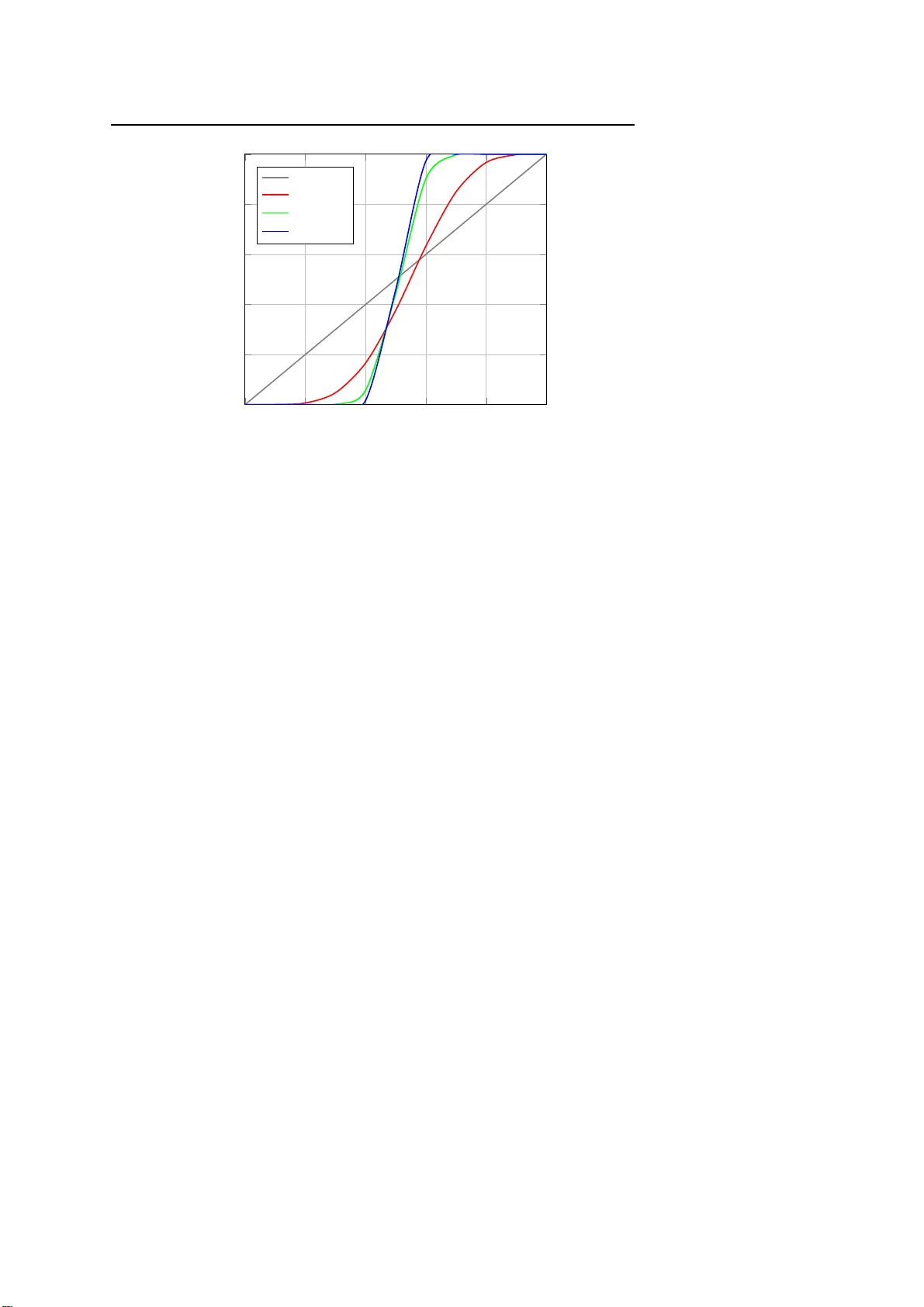
Noname man uscript No. (will be inserted b y the editor) V oting with Random Classifiers (VORA CE): Theoretical and Exp erimen tal Analysis Cristina Cornelio · Mic hele Donini · Andrea Loreggia · Mar ia Silvia Pini · F rancesca Ro s si Receiv ed: May 25, 2021 / Accepted: dat e Abstract In many machine lear ning scena rios, lo o king for the best classifier that fits a particular dataset can b e very co stly in terms of time and r esources. Moreov er, it ca n requir e deep knowledge of the specific domain. W e prop o se a new techn ique which doe s not r equire pro found exper tise in the doma in and av oids the commonly used strategy of h yper- parameter tuning a nd model selection. Our metho d is a n innov ative ens e mble tec hnique that uses voting rules over a set of rando mly-generated clas s ifiers. Given a new input sample, we interpret the output of eac h classifier as a ra nk ing over the set of p ossible classes. W e then a ggregate these output ra nkings using a voting rule, which treats them as pre fer ences o ver the classe s. W e show that o ur approach obtains This is a preprint o f an article published in Autonomous Agen ts and Multi- Agen t Systems j our nal. The final authen ticated version is av ail able online at: h ttps://doi.org/10.1007/s104 58-021-09504-y A. Loregg ia has been supported b y the H2020 ER C Pro ject “CompuLa w” (G.A.8336 47) Cristina Cornelio IBM Researc h, R¨ usc hlikon, Z ¨ uric h, Switz erland E-mail: cor@zuric h.ibm.com Michele Donini * Amazon, Berlin, Germany E-mail: donini@amazo n.com Andrea Loreggia European Universit y I nstitute, Firenze, It aly E-mail: andrea .loreggia@gmail. com Maria Silvia Pini Departmen t of Inform ation Engineering, Univ ersity of P ado v a, Italy E-mail: pini@dei.unipd.it F rancesca Rossi IBM Researc h, Y orkto wn Heigh ts, N ew Y ork, USA E-mail: francesca.rossi2@ibm.com * This w ork was mainly conducted prior joining Amazon. 2 Cristina Cornelio et al. go o d results compared to the state- of-the-art, bo th providing a theoretical analysis and an empirical ev a luation of the appro ac h on several da ta sets. Keyw ords Multi-a gen t learning · Ma c hine learning · So cial choice theor y 1 In trodu ctio n It is not easy to iden tify the b est c lassifier for a cer tain complex t ask [4, 25, 45]. Different classifiers ma y b e able to exploit better the fea tures o f different re- gions of the domain at hand, a nd consequen tly their accuracy migh t be b etter only in tha t r egion [5, 29, 40]. Moreov er, fine-tuning the classifier ’s hype r- parameters is a time-co nsuming task, whic h also req uires a deep knowledge o f the domain and a go o d exp e rtise in tuning v ario us kinds of classifiers. Indeed, the ma in appro ac hes to iden tify the hyper -parameters’ b est v alues are either manual o r based on grid search, although there ar e some a pproaches based o n random search [6]. Ho w ever, it has b een shown that in man y scenarios there is no single learning algorithm tha t can uniformly outper form the others ov er all data sets [22, 32, 46]. This observ ation led to an alter nativ e appro ac h to improv e the p erformance of a classifier , which cons ists of combining se v eral different classifiers (that is, an ensemble o f them) and taking the class prop osed by t heir combination. Over the years, many r e searchers hav e studied metho ds for construc ting go od ense mbles of cla ssifiers [16, 2 2, 30, 32, 4 2, 46], showing that indeed ensemble classifiers ar e often muc h more a ccurate than the in- dividual classifier s within the e ns em ble [30]. Clas s ifiers combination is widely applied to many different fields, such as ur ba n environmen t classifica tion [3, 53] and medical decis ion supp ort [2, 49]. In man y ca ses, the per formance of an en- semble method cannot b e easily formalize d theo r etically , but it can b e easily ev a lua ted on an exper imen tal basis in sp ecific w orking conditions (that is, a sp ecific set o f cla ssifiers, tra ining data , etc.). In this pap er w e prop ose a new ensemble c la ssifier method, c a lled V O- RA CE, whic h ag gregates randomly generated class ifie r s using voting r ules in order to provide an accura te pr ediction for a sup ervised classification task. Besides the go o d accuracy of the o verall clas s ifier, o ne of the main adv antages of using VORA CE is that it does not require specific knowledge of the domain or go o d exp ertise in fine-tuning the classifiers’ parameters . W e in terpret eac h classifier as a v oter, whose vote is its pr ediction o ver the classes, and a v oting rule agg regates s uch votes to iden tify the ”winning” cla ss, that is, the o v erall prediction of the ens e mble classifier. This use of voting rules is within the framework of maxim um likelihoo d estimators, where ea c h vote (that is, a classifier’s rank o f all classes) is interpreted as a noisy p erturbation of the cor rect ranking (that is not av ailable), so a v oting rule is a wa y to estimate this correct ranking [11, 13, 50]. T o the b est of o ur knowledge, this is the first attempt to com bine randomly generated classifiers, to b e aggreg ated in an ensem ble metho d, using voting theory to solve a supervised lear ning task without exploiting any kno wledge of the doma in. W e theor etically a nd exper imen tally show that the usage of V oting with Random Classifiers (V ORACE) 3 generic classifiers in a n ensemble en vironment can give results that are co m- parable with other state-of-the- art ensem ble metho ds. Moreover, we provide a clo sed formula to compute the p erformance of our ensemble metho d in the case of Plurality , this cor respo nds to the pr obabilit y of c ho osing the correct class, assuming that all the cla ssifiers ar e indep endent a nd have the same accu- racy . W e then relax these assumptions by defining the proba bilit y of cho osing the r igh t cla ss when the classifiers ha v e different accur acies and they are not independent. Prop erties of man y voting r ules hav e bee n s tudied extensively in the litera- ture [24, 50]. So another a dv antage o f using v oting r ules is that we can exploit that literature to mak e s ure certain des irable prop erties o f the r esulting en- semble cla s sifier hold. Bes ides the classical properties that the voting theor y communit y has co nsidered (like a non ymity , monotonicity , I IA, etc.), there may be also other proper ties not y et considered, such as v arious forms o f fairness [39, 47], whose study is facilitated by the use of voting rules . The paper is or ganized as follows. In Section 2 we br iefly desc ribe some prerequisites (a brief introduction to ensemble metho ds and voting r ules) nec- essary for what follows and an ov erview o f previo us works in this r esearch area. In Section 3 we pr esen t our a ppr oach that exploits voting theory in the ensemble clas sifier domain using neural netw orks, decision trees, a nd supp ort vector machines. In Sectio n 4 we show our exp erimental results, while in Sec- tions 5, 6 and 7 we discuss our theoretical ana ly sis: in Sectio n 5 we present the case in which a ll the clas sifiers are indep endent and with the same ac- curacy; in Section 6 w e relate our results with the Condorcet Jury Theorem also sho wing some interesting proper ties of our form ulation (e.g. mo notonicit y and b ehaviour with infinite voters/cla ssifiers); and in Section 7 we extend the results provided in Section 5 r e la xing the assumptions of having all the classi- fiers with the same-accur acy and independent b etw een each other. Finally , in Section 8 we summarize the results of the pap er and we give s o me hin ts for future work. A preliminary version of this work ha s b een published a s an extended abstract at the In ternational Co nfer ence On Autonomous A gents and Multi- Agent S ystems (AAMAS-20) [1 4]. The co de is av ailable op en source at http s://gith ub.com/aloreggia/vorace/ . 2 Bac kground and Rel ated W ork 2.1 Ensemble metho ds Ensemble metho ds com bine m ultiple classifiers in o r der to give a substantial improv ement in the pr ediction per fo rmance o f lea rning algor ithms, esp ecially for datasets which present non-informative f eatures [2 6]. Simple combinations hav e bee n studied fro m a theo r etical po in t of view, and ma ny different en- semble methods hav e b een prop osed [30]. Besides s imple standar d ensemble metho ds (such a s av eraging , blending, staking, etc.), Bagging a nd Bo osting can b e considered tw o of the main state-of-the-ar t ensemble techniques in the 4 Cristina Cornelio et al. literature [46]. In particular , Bagging [7] trains the sa me lea rning algor ithm on different subsets o f the original training set. These different training subsets are gener ated by randomly drawing, with r eplacemen t, N ins tances, where N is the origina l size o f training set. O riginal instance s may b e repeated or left out. This allows for the construction o f several different classifier s where each classifier c a n hav e sp ecific knowledge of part of the training s et. Aggrega ting the predictions o f the individual classifiers leads to the fina l ov erall pr ediction. Instead, Boo sting [21] k eeps track of the lea rning alg orithm p erformance in order to focus the tr aining attention o n instances that hav e not b een co r- rectly lear ned yet. Instead of choos ing training instances at random from a uniform distribution, it cho oses t hem in a ma nner as to fa vor the instances for which the c la ssifiers are predicting a wr ong c lass. The final overall predictio n is a weigh ted vote (pro por tio nal to the classifiers ’ training ac c uracy) of the predictions of the individual classifiers . While the a bov e are the tw o main approaches, other v a r ian ts have been prop osed, such as W agging [54], MultiBo osting [54], and O utput Co ding [17]. W e compar e our work with the state-o f-the-art in e ns em ble class ifie r s, in par - ticular XGBoos t [9 ], which is based on bo osting, and Random F ores t (RF) [27], which is based on bagging. 2.2 V oting r ules F or the purp ose of this pa p er, a voting rule is a pro cedure that allows a set of voters to collectiv ely choose one among a set of ca ndidates. V oters submit their v ote, that is, t heir preference or dering over the set o f candidates, and the voting rule aggreg ates s uc h votes to yield a final result (the winner ). In our ensemble cla s sification scena rio, the v oters are the individual classifiers and the candidates ar e the class es. A vote is a ranking of a ll the c la sses, provided by an individual cla ssifier. In the classical voting setting, given a set of n voters (or agent s) A = { a 1 , ..., a n } and m candidates C = { c 1 , ..., c m } , a pr ofile is a collection of n to tal orders o ver the set of candidates, one f or eac h voter. So, formally , a v oting rule is a map fro m a profile to a winning candidate 1 . The voting theory litera tur e includes man y voting rules, with different pr oper ties. In this pap er, w e fo cus on four of them, but the a ppr oach is applicable also to any other voting rules : 1) Pluralit y: Each voter states who the preferr ed candidate is, without pro- viding information ab out the o ther less pre fer red candidates. The winner is the candidate who is preferred b y the larg est num ber of voters. 2) Borda: Giv en m candidates, each voter gives a ranking of all candidates. Each candida te receives a scor e for each voter, bas e d o n its po s ition in the ranking: the i -th ra nk ed candidate gets the score m − i . The candidate with the largest sum of all scores wins. 1 W e assume that there is alwa ys a unique winning candidate. In case of ties b et w een candidates, we will use a predefined tie-breaking rule to c hoose one of them to be the winner. V oting with Random Classifiers (V ORACE) 5 3) Cop el and: Pairs of candidates are compared in terms of ho w man y voters prefer one or the other one, a nd the winner of suc h a pairwise comparison is the one with the largest num ber of preferences ov er the other one. The o verall winner is the candidate w ho wins the mo st pair wise comp etitions against a ll the other candidates. 4) Kem en y [28] : W e bor row a for mal definition of the rule from Conitzer et al. [12]. F or any t wo candidates a a nd b , given a ra nk ing r and a vote v , let δ a,b ( r , v ) = 1 if r and v agree on the rela tiv e ranking of a a nd b (e.g., they either bo th rank a higher, or b oth rank b higher), a nd 0 if they disag ree. Let the ag reemen t of a rank ing r with a vote v b e g iv en by P a,b δ a,b ( r , v ), the total n umber of pairwise ag r eemen ts. A K e men y ranking r maximizes the sum of the agreements with the v otes P v P a,b δ a,b ( r , v ). This is called a Kemeny consens us . A candidate is a winner o f a Kemeny election if it is the top candidate in the Kemeny consens us for that election. It is eas y to see that all the ab ov e voting rules asso ciate a scor e to each candidate (a lthough different voting rules asso ciate different sco r es), and th e candidate with the highes t score is decla red the winner . Ties ca n happen when more than one c andidate results with the highest score, we arbitra rily break the tie lexicographica lly in the exp eriments. W e plan to test the model o n different and more fair tie-breaking rules. It is imp ortant to notice that when the num b er o f candidates is m = 2 (that is, we hav e a binary classifica tion task) all the voting rules have the same outcome since they all collapse to the Ma jori ty rule, whic h e lects the candidate which ha s a ma jority , that is, mor e than half the v otes. Each of these rules ha s its adv an tages a nd dr a wbacks. V oting theory pro- vides an a xiomatic characterization of voting rules in terms of desir able prop- erties suc h as anonymit y , neutrality , etc. – for mo r e details on voting rules see [1, 48, 50]. In this pap er, w e do not exploit these prop erties to cho ose the ”b est” voting rule, but r ather w e rely on what the exp erimental ev aluation tells us ab o ut the a ccuracy o f the ensemble class ifier . 2.3 V oting for ensemble metho ds Preliminary tec hniques from v oting theory have alrea dy b een used to co m bine individual classifier s in order to improve the p erformance of some ensemble classifier metho ds [5, 1 8, 22, 31]. Our approach differs from these methods in the w ay classifie r s are generated and ho w the outputs o f the individual clas- sifiers ar e aggregated. Although in this pap er we report r esults only agains t recent ba gging and b o osting techniques of e ns em ble classifiers, w e compared our approach with the other existing approaches as w ell. More adv anced work has b een done to study the us e o f a specific voting rule: the use of majority to ensemble a profile of clas sifiers has b een inv estigated in the work o f La m and Suen [34], wher e they theoretically analyz e d the per formance of ma jority vot- ing (with r eje ction if the 50% o f consensus is not rea c hed) when the classifier s are ass umed indepe ndent. In the work of Kunchev a et al. [33], they provide 6 Cristina Cornelio et al. upper and lo wer limits on the ma jority vote accur a cy foc us ing on dep e ndent classifiers .W e perform a similar analysis of the dep endence betw een classifier but in the mor e complex case of plur alit y , with als o an ov erview o f the genera l case. Although ma jor it y seems to be easier to ev aluate compared to plur al- it y , there hav e b een some attempts to study plurality a s well: Lin X. and S. [37] demonstrated so me int eresting theoretical results for independent classi- fiers, and Mu et al. [41] extended their work pro viding a theo r etical analysis of the probability of ele c ting the correct c la ss by an ensemble using plur alit y , or plurality with re jectio n, as well as a s to chastic analysis of the formula, and ev a lua ting it on a datas et for human recognition. How ever, we have noted an issue with their pro of: the a uthors assume indepe ndence betw een the random v ar iable ex pressing the total num b er of v otes receiv ed b y the correct class and the o ne defining the maximum num ber of votes among all the wro ng classes. This false ass umption lea ds to a wrong final form ula (the pro of can b e found in Appendix A ). In our w ork, we provide a form ula that exploits genera ting functions and that fixes the problem o f Mu et al. [41], based on a different approach. Moreover, we pr o vide pr oo f for the tw o gener al cases in whic h the accuracy of the individual classifiers is not homogene o us, and where classifier s are not independent. F urthermore, our ex perimental analysis is mor e compre- hensive: not limiting to plur alit y and considering ma n y datasets of different t yp es. There are a ls o some approa c hes that use Bor da c ou n t for ense mble metho ds (see for example the work of v an Erp and Schomak er [1 9]). Mor e- ov er, v oting rules have b een applied to the sp ecific ca se of Bagging [35, 36]. How ev er, in Leon et al. [35], the a uthors co m bine only classifier s fro m the same family (i.e., Naive Bayes classifier) witho ut mixing them. A differe n t p ersp ective comes from the work o f De Condorcet et a l. [15] and further improv ements [11, 13, 55] where the basic assumption is that there a lways exists a correct r anking of the alternatives, but this ca nnot b e observed directly . V oters derive their preferences ov er the a lternativ es fro m this ra nking (pertur bing it with noise). Scor ing v oting r ule s are prov ed to b e maximum likelihoo d estimato rs (MLE). Under this a pproach, one computes the likeliho o d of the given preference profile for each po ssible state of the world, tha t is, the true rank ing of the alternatives and the b est r anking of the alternatives are then the ones that have the highest likelihoo d of pro ducing the giv en profile. This mo del aligns v ery w ell with our prop osal and justifies the us e of v oting rules in the a g gregation of classifiers’ predictio n. More o ver, MLEs giv e also a justification to the p erforma nce of ensembles where v oting rules are used. 3 V ORA CE The ma in idea of VORA CE (VOting with RAndom ClassifiEr s) is that, given a sample, the output of ea ch classifier c a n b e seen as a ranking ov er the av a ila ble classes, where the ranking order is given by the classifier’s expe cted pr obabilit y that the sample belong s to a class . Then a voting rule is used to aggr egate these V oting with Random Classifiers (V ORACE) 7 orders and declare a class as the ” winner”. VORA CE generates a profile of n classifiers (where n is an input pa rameter) by randomly choo sing the t ype of each classifier amo ng a set of predefined ones. F or ins tance, the classifier type can b e drawn b et w een a decisio n tree or a neural netw ork. F or ea c h c la ssifier, some of its h yper -parameters v alues are chosen at random, where the c hoice of which hyper-pa rameters and which v alues are randomly c hosen dep ends on the t yp e of the classifier. When all classifier s ar e generated, they are trained using the same set of training sa mples . F or each clas s ifier, the output is a vector with as ma ny elements as the classes , where the i -th element represents the probability that the classifier assigns the input s ample to the i -th class. Output v alues are ordere d fro m the hig hest to the smallest one, a nd the o utput of ea ch classifier is interpreted as a ranking ov er the classe s , where the class with the highest v alue is the first in the rank ing , then we ha ve the clas s that has the second hig hest v alue in the output o f the classifier , and so o n. These ra nkings are then aggregated using a voting r ule. The winner of the election is the class with the higher scor e. This co rresp onds to the prediction of V ORA CE. Ties can o ccur when more than one clas s gets the s ame score fr o m the voting rule. In these case s , the winner is elected using a tie-breaking r ule, which choos es the candidate that is most preferred b y the cla ssifier with the highest v alidation accuracy in the profile. Example 1 Let us consider a profile comp osed by the output vectors of three classifiers , say y 1 , y 2 and y 3 , o ver four candida tes (class es) c 1 , c 2 , c 3 and c 4 : y 1 = [0 . 4 , 0 . 2 , 0 . 1 , 0 . 3 ], y 2 = [0 . 1 , 0 . 3 , 0 . 2 , 0 . 4 ], and y 3 = [0 . 4 , 0 . 2 , 0 . 1 , 0 . 3 ]. F o r instance, y 1 represents the prediction of the first classifier, which co uld predict that the input sample be lo ngs to the fir s t class with probability 0 . 4, to the second class with probability 0 . 2, to the third class with probability 0 . 1 and to the four th class with probability 0 . 3. F rom the pr evious predictions we can derive the corr espondent ranked order s x 1 , x 2 and x 3 . F or instance, fr om prediction y 1 we can see that the first cla ssifier prefers c 1 , then c 4 , then c 2 and then c 3 is the less pre fer red cla ss for the input s ample. Th us we hav e: x 1 =  c 1 , c 4 , c 2 , c 3  , x 2 =  c 4 , c 2 , c 3 , c 1  and x 3 =  c 1 , c 4 , c 2 , c 3  . Using Bo rda, class c 1 gets 6 p oin ts, c 2 gets 4 p oints, c 3 gets 1 p oint and c 4 gets 7 p oin ts. Therefore, c 4 is the winner, i.e. VORA CE outputs c 4 as the predicted cla s s. On the other hand, if w e used Pluralit y , the winning class would be c 1 , since it is preferred by 2 out of 3 voters. Notice that this metho d do es not need an y knowledge of ar chitecture, t yp e, or parameters , of the individual classifiers. 2 4 Exp erimen tal Results W e c onsidered 23 datasets from the UCI [43] rep ository . T able 1 g iv es a brief description of these da tasets in terms of num ber of ex amples, n umber of fea- tures (where some features a re categorical and others are n umerical), whether 2 Code a v ailable at https://gith ub.com/aloreggia/vorace/ . 8 Cristina Cornelio et al. Dataset #Examples #Categorical #Numerical Missing #Classes anneal 898 32 6 y es 6 autos 205 10 15 y es 7 balance-s 625 0 4 no 3 breast-cancer 286 9 0 y es 2 breast-w 699 0 9 y es 2 cars 1728 6 0 no 4 credit-a 690 9 6 y es 2 colic 368 15 7 yes 2 dermatology 366 33 1 y es 6 glass 214 0 9 no 5 haberman 306 0 3 no 2 heart-statlog 270 0 13 no 2 hepatitis 155 13 6 y es 2 ionosphere 351 34 0 no 2 iris 150 0 4 no 3 kr-vs-kp 3196 0 36 no 2 letter 20,000 0 16 no 26 lymphogra 14 8 15 3 no 4 monks-3 122 6 0 no 2 spam base 4,601 0 57 no 2 v ow el 990 3 10 no 11 wine 178 0 13 no 3 zoo 101 16 1 no 7 T able 1 Descri ption of th e datasets. # V oters Avg Profile Borda Plurality Copeland Kemeny Sum Best C. 5 0.8599 (0.1021) 0.8864 (0.1043) 0.8885 (0.1052) 0.8885 (0.1051) 0.8886 (0.1050) 0.8864 (0.1116) 0.8720 (0.119 9) 7 0.8652 (0.0990) 0.8942 (0.0995) 0.89 66 (0.1005 ) 0.8965 (0.1007) 0.8966 (0.1007) 0.8942 (0.1052) 0.8689 (0.1168) 10 0.8626 (0.0988) 0.8990 (0.0979) 0.9007 (0.0998) 0.9004 (0.1001) 0.9008 (0.1007) 0.8985 (0.1050) 0.8667 (0.119 6) 20 0.8615 (0.0965) 0.9015 (0.0968) 0.90 43 (0.0977 ) 0.9036 (0.0981) 0.9033 (0.0987) 0.8992 (0.1065) 0.8655 (0.120 3) 40 0.8630 (0.0960) 0.9044 (0.0958) 0.90 66 (0.0967 ) 0.9060 (0.0968) 0.9058 (0.0969) 0.9006 (0.1050) 0.8651 (0.118 3) 50 0.8633 (0.0957) 0.9044 (0.0962) 0.90 68 (0.0970 ) 0.9060 (0.0970) 0.9062 (0.0972) 0.8995 (0.1076) 0.8655 (0.120 4) Avg 0.8626 (0.0981) 0.8983 (0.0987) 0.90 06 (0.0998 ) 0.9002 (0.0998) 0.9002 (0.1001) 0.8964 (0.1070) 0.8673 (0.119 2) T able 2 Average F1-scores (and standard deviation), v aryi ng the n umber of voters, a v er- aged o v er all datasets. there are missing v a lues for some features, and n umber of class es. T o genera te the individual classifiers, we use three classification algorithms: Decision T rees (DT), Neural Netw orks (NN), a nd Supp ort V ector Mach ines (SVM). Neural net w orks are g enerated by choo sing 2, 3 or 4 hidden layers with equal pr obabilit y . F or eac h hidden lay er, the n um b er of no des is sampled ge- ometrically in the r ange [ A, B ], whic h means computing ⌊ ( e x ) ⌋ where x is drawn uniformly in the int erv al [log( A ) , log( B )] [6]. W e cho ose A = 16 and B = 128 . The activ atio n function is chosen with equal pr obabilit y b et w een the rectifier function f ( x ) = max (0 , x ) and the h ype r bolic tangent function. The maximum n um be r of ep ochs to train each neur al net w ork is set to 100. An early stopping callbac k is used to pr ev ent the training phase to con tinue even when the accuracy is not improving and w e set the patience para meter to p = 5 . Batch s iz e v a lue is adjusted to respect the size of the dataset: giv en a training set T with size l , the batch size is set to b = 2 ⌈ log 2 ( x ) ⌉ where x = l 100 . V oting with Random Classifiers (V ORACE) 9 Dataset Ma jori t y Sum RF XGBoost breast-cancer 0.7356 (0.0947) 0.7151 (0.0983) 0.713 4 (0.0397) 0.7000 (0.0572) breast-w 0.9645 (0.0133) 0.9610 (0.0168) 0.9714 (0.0143) 0.9613 (0.0113) colic 0.8587 (0 .0367) 0.8573 (0.0514) 0.8507 (0.0486) 0.875 0 (0.0 534) credit-a 0.8590 (0.0613) 0.8478 (0.0635) 0. 8710 ( 0.0483) 0.8565 (0.0763) haberman 0.7337 (0.0551) 0.6994 (0.0765) 0. 7353 ( 0.0473) 0.7158 (0.0518) heart-statlog 0.8070 (0.0699) 0.7885 (0.0797) 0. 8259 ( 0.0621) 0.8222 (0.0679) hepatitis 0.8385 (0.0903) 0.8377 (0.0955) 0. 8446 ( 0.0610) 0.8242 (0.0902) ionosphere 0.9435 (0.0348) 0.9366 (0.0344) 0.9344 (0.0385) 0.9260 (0 .0427) kr-vs-kp 0.9958 (0.0044) 0.9960 (0.0044) 0.9430 (0.0139) 0.9562 (0.0174) monks-3 0.9182 (0.0712) 0.9115 (0.0748) 0. 9333 ( 0.0624) 0.9333 ( 0.0624) spamba se 0.9416 (0.0105) 0.8801 (0.1286) 0.9100 (0.0137) 0.9294 (0 .0112) Ave rage 0.8724 (0.0493) 0.8574 (0.0658) 0.8666 (0 .0409) 0.8636 ( 0.0493) T able 3 Performances on binary datasets: A v erage F1-scores (and standard deviation). Best p erformance in bold. On binary datasets, all the v oting rules b eha ve as ma j orit y voting rule. Dataset Borda Plurality Copeland Kemen y Sum RF XGBoost anneal 0.991 7 (0.0138) 0.9876 (0.0200) 0.9876 (0.0200) 0.9880 (0.0194) 0.9894 (0.0174) 0.8471 (0.0122) 0.9912 (0.0080) autos 0.8021 (0.06 69) 0. 7848 (0 .0794) 0.7803 (0.0768) 0.7832 (0.0771) 0.8095 (0.0749) 0. 6890 (0.0743) 0. 8298 (0.0744) balance 0.9016 (0.0366 ) 0. 9208 (0.0311) 0.9069 (0.0292) 0.9082 (0.0297) 0.8911 (0.0376) 0.8561 (0.0540) 0.8578 (0.0441) cars 0.9916 (0.0079) 0.9932 (0.0054) 0.9931 (0.0054) 0.9934 (0.0053) 0.9931 (0.0048) 0.7928 (0.0300) 0.8935 (0.0266) dermatology 0.9819 (0.0192) 0.9769 (0.0206) 0.9769 (0.0206) 0.9766 (0.0209) 0.9783 (0.0196) 0.9699 (0.0256) 0.9755 (0.0189) glass 0.9708 (0.0364) 0.9602 (0.0319) 0.9607 (0.0291) 0.9611 (0.0287) 0.9742 (0.02 68) 0.9535 ( 0.0295) 0.9719 (0.0313) iris 0.9473 (0.0576) 0.9473 (0.0576) 0.9473 (0.0576) 0.9480 (0.0570) 0.9527 (0.0519) 0.9533 (0.0521) 0.9 600 (0.0442) letter 0.9311 (0.01) 0.9590 (0.01) 0.9545 (0.01) - 0.9627 (0.01) 0.604 4 (0.01) 0.8832 (0.01) lymphography 0.8461 (0.0983) 0.8630 (0.085 1) 0.8624 (0.0843) 0.8604 (0.0875) 0.8529 (0.0925) 0.8586 (0.0691) 0.8519 (0.0490) vo wel 0.9476 (0.0232) 0.9862 (0.01 10) 0.9860 (0.0116) 0.9860 (0.0114) 0.9862 (0.01 19) 0.7333 ( 0.0323) 0.8323 (0.0333) wine 0.9656 (0.0537) 0.9789 (0.0331) 0.9783 (0.0342) 0.9783 (0.0342) 0.9806 (0.0380) 0.9889 (0.0 222) 0.9611 (0.055 8) zoo 0.9550 (0.0497) 0.9550 (0.0517) 0.9560 (0.0496) 0.9590 (0.0492) 0.9500 (0.0640) 0.9500 (0.0500) 0.9700 ( 0.0640) Average 0.9365 (0.0421) 0.9413 (0.0388) 0.9396 (0.0380) 0.9402 (0.0382) 0.9416 (0.0399) 0.8720 (0.0410) 0.9177 (0.0409) T able 4 Performances on multiclass datasets: Average F1-scores (and standard deviation). Best performance in b old. Decision trees are generated b y c ho osing betw een the e ntr opy and gini criteria with equal probability , and with a maximal depth unifor mly sampled in [5 , 25]. SVMs are genera ted by choosing rando mly b et ween the rbf and p oly ker- nels. F or bo th t yp es, the C factor is dr a wn geometric a lly in [2 − 5 , 2 5 ]. If the t yp e of the kernel is p oly , the co efficient is sa mpled at ra ndom in [3 , 5]. F or rbf kernel, the gamma parameter is set to auto. W e used the average F1-sco re of a classifier ensemble a s the ev aluation metric, for all 23 different data sets, since the F1-score is a be tter measure to use if we need to seek a ba lance b etw een Precision and Recall. F or each dataset, w e tr ain and test the ensemble metho d with a 10- fold cro ss v alidation pro cess. Additionally , for each dataset, exp erimen ts are p erformed 10 times, leading to a tota l of 100 runs for each method ov er each dataset. This is done to ensure g reater stability . The voting rules co nsidered in the exp eriments are Plurality , Borda, Cop eland and K e meny . In or de r to compute the Ke meny cons ensus, we leverage the implementa- tion of the Kemeny method for rank aggreg ation of inco mplete rank ings with ties that is av ailable with the Python pack a g e named cor ank co 3 . The pack- age provides s ev eral methods for computing a Kemen y consensus. Finding a 3 The pac k age is a v ailable at https ://pypi.org /project/corankco/ . 10 Cristina Cornelio et al. Kemeny consensus is computationally ha rd, es pecially when the n umber o f candidates gr o ws. I n order to ensur e the feasibilit y of the exp eriments, we compute a K e men y c onsensus using the exact algorithm with ILP Cplex when the n um b er o f c lasses | C | ≤ 5 , other wise we e mplo yed the consensus compu- tation with a heuris tic (s e e pack age do cumen tation for further details). W e compare the p erformance of VORA CE to 1) the average p erformance of a profile of individual classifiers , 2) the per formance of the b est classifier in the profile, 3) tw o state-of-the-a rt metho ds (Random F orest and XGBoo st), a nd 4) the Sum metho d (also called weighte d aver aging ). The Su m method computes x Sum j = P n i x j,i for each individual classifier i and for e a c h class j , where x j,i is the probabilit y tha t the sample b elongs to cla s s j predicted b y c la ssifier i . The winner is the one with the maximum v alue in the sum vector: arg max x Sum j . W e did not co mpare V ORACE to a more sophisticated version of Sum , such as c onditional aver aging , since they a re not applicable in our case, r equiring additional knowledge of the domain which is out of the scop e of our work. Bo th Random F orest a nd XGBo ost cla ssifiers ar e gener ated with the same num ber of t rees as the n umber of classifier s in the profile, all the remaining para meters are gener ated using default v alues. W e did not compa re to stacking b ecause it would require to man ually iden tify the c orrect structure of the s equence of classifiers in order to obtain comp etitive re s ults. An optimal str uc tur e (i.e., a definition o f a second level meta-classifier) can b e defined by an exp ert in the domain at hand [8], and this is out of the scop e o f our work. T o study the accuracy o f o ur metho d, we p erformed three kinds o f ex per- imen ts: 1 ) v arying the n umber o f individual classifier s in the profile and av- eraging th e perfor mance ov er all datasets, 2) fixing the num ber of indiv idua l classifiers and a nalyzing the perfor mance on each dataset and 3) considering the in tro duction o f mo r e complex classifiers as ba s e clas sifiers for VORA CE. Since t he first exp eriment shows that the b est accuracy of the ensemble o ccurs when n = 50, we use only this size for the second and third exp erimen ts. 4.1 Exp eriment 1: V a rying the n umber of voters in the ensemble The aim of the first ex p eriment is tw ofold: on one hand, w e want to show tha t increasing the n um b er of classifiers in the profile leads to an improvemen t of the perfo rmance. On the other hand, we wan t to show the effect of the aggre g ation on per formance, compa red with the best class ifier in the profile and with the av erage classifier’s p erformance . T o do that, we first ev alua te the ov erall av erage accur acy of VORA CE v arying the num ber n of individual classifiers in the profile. T able 2 presents the per formance of each ensemble for different num bers of classifiers , sp ecifically n ∈ { 5 , 7 , 10 , 20 , 40 , 50 } . Pluralit y , Cop eland, and Kemeny voting rules hav e their best ac c uracy for V ORACE when n = 50. W e set the system to stop the ex periment after the time limit of one week, this is why we stop when n = 50. W e are pla nning to run exper imen ts with la rger time limits in or der to understand whether the system shows that the effect o f the profile’s size diminishes at so me p oint. In T able 2, we rep ort V oting with Random Classifiers (V ORACE) 11 the F1 -score and the standard deviation of VORA CE with the considere d voting r ules. The la st line o f the table presen ts the a verage F1-sco re for each voting rule. The dataset “letter” was not co nsidered in this test. Increasing the n um b er of cla ssifiers in the ensemble, all the co nsidered voting rules sho w an increase of the p erformance, sp ecifically the higher the nu mber of the classifier s the higher the F1-sco re of V ORACE. How ev er, in T able 2 we can obser v e that the p erforma nce is slightly incre- men tal when we increase the num be r of classifiers. This is due to the fact that in this par ticula r exp eriment the accuracy of every single classifier is usually very high (i.e., p ≥ 0 . 8), thus the ensemble has a reduced con tribution to the aggre g ated r e s ult. In general this is not the ca se, esp ecially w he n we hav e to deal with “harder ” datasets where the acc uracy p of single classifiers is low er. In Section 5, we will explore this case and we will se e that the n umber of clas- sifiers has a greater impact on the a ccuracy of the ensem ble when the accuracy of the classifier s on av erage is low (e.g., p ≤ 0 . 6 ). Moreov er, it is worth noting that the computational cost of the ensemble (bo th training and testing) increase s linearly with the n umber o f classifier s in the pr ofile. Thus, it is co n venien t to consider more classifiers, es pecially when the a ccuracy of the single classifiers is p o or. Th us, overall, the inc r ease in the nu mber of classifier s has a pos itiv e effect o n the p erforma nce of VORA CE, as exp ected given the theoretical analysis in Section 5 4 . F or each v oting rule, we also compared VORA CE to the av erage per for- mance of the individual classifier s and the b est classifier in the pr o file, to understand if V ORACE is be tter than the be st classifier, o r if it is just b etter than t he average classifiers’ ac c ur acy (a round 0 . 86 ). In T able 2 we can see that V ORACE always b ehav es b etter than bo th the best classifier and the profile’s av erage. Mor eov er, it is in teresting to obser ve that Plura lit y p erfor ms b etter on av erage than more complex voting rules like Borda and Co peland. 4.2 Exp eriment 2: Comparing with existing metho ds F or the second exp eriment, we set n = 50 and we compare V ORACE (us- ing Ma jority , Borda, P luralit y , Cop eland, and Kemeny) with Sum, Random F orest (RF), a nd XGBoost in each dataset. T able 3 r epor ts the p erformances of VORA CE on binary da ta sets where all the v oting r ules collapse to Ma jor- it y v oting. V ORA CE perfo rmances ar e very clo se to the state-of-the-art. W e try to use Kemeny on the dataset “ letter” but it exceeds the time limit of one week and th us it w as not p ossible to compute the av erage. In order to make the average v alues comparable (last row of T a ble 4), per formances o n the datase t “ letter” were not consider ed in the co mputation of the average v alues for the other metho ds. T able 4 r eports the per fo rmances on datasets that hav e m ultiple cla sses: whe n the num b er of clas ses incr eases V ORACE is still stable and b ehav es very similarly to the sta te-of-the-art. The similarity 4 How ev er, the experiments do not satisfy the independence assumption of the theoretical study 12 Cristina Cornelio et al. among the performance s is promising for the sys tem. Indeed, RandomF ores t and X GBo ost reach better perfor mances on some datasets and they can b e improv ed on over by optimizing t heir h yper parameters. But, this exper imen t shows tha t it is p ossible to r each very s imila r per formances using a very simple metho d as V ORACE is. This means that usage of V ORACE does not req uire any optimization of hyper parameters whether it is do ne manually o r automat- ically . The importa nce of this prop ert y is corrob orated by a recent line of w ork by [52] that suggests how industry and aca demia should fo cus their effor ts on developing to ols that r educe or av oid hyper parameters’ optimization, resulting in simpler metho ds that are a lso mo r e susta inable in terms of e nergy and time consumption. Moreov er, Plurality is b oth more time and space e fficien t s ince it needs a sma ller amount of infor mation: for e a c h clas sifier it just needs the most preferred ca ndida te instead of the whole r anking, contrarily to other methods such as Sum. W e also per formed t wo a dditional v ariants o f these experiments, one with a weight ed v ersion o f the v oting rules (where the weigh ts are the classifiers ’ v a lida tion accuracy), and the o ther o ne b y training eac h classifier on different por tions of the da ta in or der to increase the indep endence b et ween them. In bo th experiments, the results are v ery similar to the ones reported here. 4.3 Exp eriment 3: In tro ducing complex classifiers in the profile The goal of the third exp eriment is to understand whether using complex clas- sifiers in the profile (such a s using an ense m ble o f ensembles) would produce better final per formances. F o r this purp o se, w e compar ed VORA CE with stan- dard ba se classifiers (desc ribed in Sectio n 3) with three differen t versions of V ORACE with complex ba s e classifiers: 1) V ORACE with only Random F or- est 2) VORA CE with only X GBo ost and 3) V ORACE with Random F or est, X GBo ost and s tandard ba se cla ssifiers (DT, SVM, NN). F or simplicity , we used the Plura lit y voting rule, s ince it is the most ef- ficient metho d and it is one of the voting r ules that gives b etter results. W e fixed the nu mber o f v oters in the profiles to 50 and w e sele cted the parameters for the simple cla ssifiers for VORA CE as descr ibed at the b e- ginning o f Section 4. F or Random F orest, par ameters w ere drawn uniformly among the following v alues 5 : b o otstr ap b et ween T rue a nd F alse , m ax depth in [10 , 20 , . . . , 100 , N one ], max fe atur es b et ween [ a u to, sq rt ], min samples le af in [1 , 2 , 4], min samples spl it in [2 , 5 , 10], and n estimators in [10 , 20 , 5 0 , 100 , 20 0 ]. F or X GB o os t instead the parameters w ere dr a wn unif ormly among the follo w- ing v alues: max depth in the range [3 , 25], n estimators equals th e n um b er of classifiers , subsample in [0 , 1 ], and c olsampl e bytr e e in [0 , 1]. The results of the compariso n betw een the different versions o f VORA CE a re provided in T able 5. W e can observe that the p erformance of V ORACE (co lumn ”Ma jority” o f 5 Pa rameters’ n ames and v alues r efer to the Python’s modules: R andomForest Classifier in s klearn.ense mble and xgb in xgboos t . V oting with Random Classifiers (V ORACE) 13 T able 3 and column ” Plurality” of T able 4) is not significa n tly improv ed by us- ing more complex class ifiers a s a base for the profile. It is interesting to notice the effect of VORA CE on t he agg regation of RF with res p ect to a single RF. Comparing the results in T able 3 and 4 (RF column) with results in T able 5 (V ORACE with only RF column), one can notice that RF is p ositively a ffected by the aggregation on ma n y datasets (on all the datasets the improv emen t is on av erage 5%), esp ecially on those with m ultiple classes. Moreov er, the im- prov ement is significan t in man y of them : i.e. on “letter” datas et we hav e an improv ement o f more than 35 %. This effect can be explained by the random aggre g ation of trees used by the RF algorithm, where the goal is to reduce the v ariance of the single classifier. In this sense, a principled a ggregation of different RF models (a s the one in V ORACE) is a correct wa y to b o o st the final p erformance: dis tinct RF mo dels a ct differently o ver sepa rate parts of the domain, pro viding VORA CE with a g o o d set of weak cla ssifiers – see Theorem 3. W e sa w in th is section that this more complex v ersion o f V O RA CE doe s not provide any s ig nifican t adv an tage, in terms of per formance, compared with the standard one. T o conclude, we thus suggest using V O RA CE in its standard version without adding complexity to the ba s e class ifiers. dataset VORA CE wi th VORA CE with V ORACE with RF & XGBoost only RF only XG Bo ost anneal 0. 9937 (0.01) 0.9921 ( 0.01) 0.9893 (0.01) autos 0.8095 ( 0.09) 0.7969 (0.10) 0 .7916 (0.08) balance 0.8998 (0.02) 0.8456 (0.03) 0.804 0 (0.04) breast-cancer* 0.7573 ( 0.04) 0.7485 (0.06) 0 .7394 (0.06) breast-w* 0.9654 ( 0.02) 0.9744 (0.02) 0 .9605 (0.03) cars 0.9887 ( 0.01) 0.9547 (0.01) 0 .9044 (0.05) colic* 0.8668 ( 0.04) 0.8766 (0.04) 0 .8638 (0.04) credit-a* 0.8737 (0.03) 0.8691 (0.03) 0.8712 (0.03) dermatology 0.9749 ( 0.02) 0.9765 (0.02) 0 .9805 (0.02) glass 0.9761 ( 0.03) 0.9740 (0.04) 0.977 0 (0.03) haberman* 0.7338 (0.04) 0. 7168 (0.04) 0.7286 (0.02) heart-statlog* 0.8315 (0.09) 0.8352 (0.09) 0.8248 (0.08) hepatitis* 0.8215 (0.07) 0.8091 (0.05) 0.8105 (0.08) ionosphere* 0.9349 ( 0.04) 0.9272 (0.05) 0 .9347 (0.04) iris 0.9627 (0.05 ) 0.9593 (0.04) 0.9593 (0.05) kr-vs-kp* 0.9953 (0.00) 0.9869 (0.01) 0 .9892 (0.01) letter 0.9632 ( 0.01) 0.9622 (0.01) 0.926 5 (0.01) lymphograph y 0.8700 ( 0.10) 0.8306 (0.15) 0 .8412 (0.14) monks-3* 0.9156 (0.07) 0.9340 (0.06) 0 .9037 (0.07) spamb ase* 0.9437 ( 0.01) 0.9439 (0.01) 0.93 37 (0.01) v ow el 0.9834 ( 0.01) 0.9691 (0.02) 0.90 86 (0.03) wine 0.9851 (0.03) 0.9764 (0.04) 0.9796 (0.04) zoo 0.9535 ( 0.05) 0.9589 (0.05) 0 .9231 (0.06) Ave rage 0.9130 (0.04) 0.9051 (0.04 ) 0.8933 (0.04) T able 5 Average F1-s cores (and standard deviat ion). * denot es binary da tasets. 14 Cristina Cornelio et al. In other exp eriments, w e als o see tha t the probability of cho osing the cor- rect class decreases if the n umber of clas ses incr eases. This means that the task bec omes mor e difficult with a la r ger num ber o f classes . 5 Theoretical analysis: Indep enden t classifiers with the same accurac y In t his section we theoretically analyze the probability to predict the cor r ect lab el/class o f o ur ensemble metho d. Initially , we c o nsider a simple scenario with m cla s ses (the candidates) and a profile of n independent classifier s (t he voters), where ea c h classifier has the same probability p of correc tly c la ssifying a given instance. The independence assumption hardly fully holds in practice, but it is a natural simplification (commonly adopted in literature) used for the sake of analys is. W e assume that the system uses the P lurality v oting rule. This is justified by the fac t that Plurality provides better results in o ur exp erimental analysis (see Section 4) a nd th us it is the one we suggest to use with V ORACE. Mo re- ov er, Plurality has also the adv antage to r equire very little information from the individual classifier s and also b eing computatio nally efficient. W e are in terested in computing the pro babilit y that V ORACE chooses the cor r ect class. This probability corresp onds to the a ccuracy of VORA CE when considering the single cla ssifiers a s black boxes, i.e., knowing only their accuracy without any other informa tion. The res ult presen ted in the fo llo wing theorem is espec ially p ow erful b ecause it shows a closed formula that only requires for the v alues of p , m , and n to b e k no wn. Theorem 1 The pr ob abili ty o f ele ct ing the c orr e ct class c ∗ , among m classes, with a pr ofile of n classifiers, e ach one with ac cur acy p ∈ [0 , 1] , using Plur ality is given by: T ( p ) = 1 K (1 − p ) n n X i = ⌈ n m ⌉ ϕ i ( n − i )!  n i   p 1 − p  i (1) wher e ϕ i is define d as the c o efficient of t he monomial x n − i in the exp ansion of the fol lowing gener ating function: G m i ( x ) =   i − 1 X j =0 x j j !   m − 1 and K is a normalization c onstant define d as: K = n X j =0  n j  p j ( m − 1) n − j (1 − p ) n − j . V oting with Random Classifiers (V ORACE) 15 Pr o of The formula c a n b e rewritten as: T ( p ) = 1 K n X i = ⌈ n m ⌉  n i  p i ϕ i ( n − i )!(1 − p ) n − i and co r resp onds to the sum o f the pr obabilit y of all the p ossible differen t profiles v otes that elect c ∗ . W e per fo rm the sum v arying i , an index that indicates the n umber o f classifiers in the profile that vote for the correct lab el c ∗ . This num b er is b etw een ⌈ n m ⌉ (since if i < ⌈ n m ⌉ that profile cannot elect c ∗ ) and n where all the clas sifiers v ote fo r c ∗ . The binomial factor expresses the nu mber of p ossible po sitions, in the or der ed pro file of size n , of i classifiers that votes for c ∗ . This is multiplied by the proba bilit y of these classifier s to vote c ∗ , that is p i . The factors ϕ i ( n − i )! corresp ond the n um b er of poss ible combinations of v otes of the n − i classifiers (on the other ca ndidates differen t from c ∗ ) tha t e nsure the winning of c ∗ . This is computed as the n umber of po ssible co m binations of n − i ob jects extracted from a set ( m − 1) ob jects, with a b ounded num b er of rep etitions ( b ounded by i − 1 to ensure the winning of c ∗ ). The formula to use for coun ting the nu mber of combinations of D ob jects extracted from a set A ob jects, with a bounded num ber of rep etitions B , is: ϕ i D !. In our ca se A = m − 1 is the n umber of ob jects, B = i − 1 is the maximum num ber of rep etitions and D = n − i the positions to fill and ϕ i is the co efficien t of x D in the expansion of the following gener ating function:   B X j =0 x j j !   A A = m − 1 = = = = = ⇒ B = i − 1   i − 1 X j =0 x j j !   m − 1 = G m i ( x ) . Finally , the facto r (1 − p ) n − i is the probability that the remaining n − i clas- sifiers do not elect c ∗ . ⊓ ⊔ F or the sake of comprehension, we give an example that descr ibes the computation of the probability o f ele c ting the correct class c ∗ , as formalized in Theorem 1. Example 2 Considering an ensem ble with 3 classifiers (i.e., n = 3), each o ne with accur a cy p = 0 . 8. The n um b er of cla s ses in the da taset is m = 4 . The probability of c ho osing the correc t cla ss c ∗ is given b y the formula in Theo- rem 1. Sp e cifically: T ( p ) = (1 − 0 . 8 ) 3 1 K 3 X i =1 ϕ i · (3 − i )!  3 i   0 . 8 1 − 0 . 8  i where K = 1 . 728 . In or de r to compute the v alue of each ϕ i , we hav e to compute the co e fficien t of x 3 − i in the expansion of the generating function G 4 i ( x ). F or i = 1 : W e have G 4 1 ( x ) = 1, and we ar e interested in the co e fficien t o f x n − i = x 2 , th us ϕ 1 = 0. 16 Cristina Cornelio et al. F or i = 2 : W e have G 4 2 ( x ) = 1 + 3 x + 3 x 2 + x 3 , and w e a re interested in the co efficien t of x n − i = x 1 , th us ϕ 2 = 3. F or i = 3 : W e hav e G 4 3 ( x ) = 1 + 3 x + 9 2 x 2 + 4 x 3 + 9 4 x 4 + 3 4 x 5 + 1 8 x 6 , and we are in terested in the co efficien t of x n − i = x 0 , thus ϕ 3 = 1. W e c an now co mpute the pro babilit y T ( p ): T ( p ) = 0 . 008 1 . 728 · ( ϕ 1 · (2)!  3 1  · 4 + ϕ 2 · (1)!  3 2  · (4) 2 + ϕ 3 · (0)!  3 3  · (4) 3 ) = 0 . 963 . The result says that VORA CE with 3 clas sifiers (each one with accur a cy p = 0 . 8) has a probability of 0 . 963 of choosing the corre c t class c ∗ . It is w orth noting that T ( p ) = 1 when p = 1, meaning that, when all the classifiers in the ensem ble alw ays predict the right class, our ensem ble method alwa ys outputs the cor rect class a s well 6 . Mo reov er, T ( p ) = 0 in the s ymmetric case in whic h p = 0 , that is when all the cla ssifiers a lw ays predict a wrong class. Note that the indep endence assumption considered ab o ve is in line with previous studies (e.g., the same ass umption is made in [10, 55]) a nd it is a necessary s implification to obtain a closed for m ula to co mpute T ( p ). Moreover, in a realistic scenario, p ca n b e interpreted as representing the low er b ound of the accuracy of the clas sifiers in the pro file. It is easy to see that under this int erpreta tion the v alue of T ( p ) as w ell represents a low er bound of the probability of electing the co rrect class c ∗ , given m av ailable class e s , and a profile of n classifiers. Although this theoretical result holds in a res tricted scenario and with a sp ecific voting rule, as w e alrea dy noticed in our exper imen tal ev aluation in Section 4, th e pr obabilit y of cho o sing the correct class is alw ays greater than or equal to each individual classifier s’ accura cy . It is w orth noting that the scena r io co nsidered ab ov e is similar to the o ne analyzed in the Condor c et Jury The or em [10], which states that in a scenario with tw o candidates where each v oter has probability p > 1 2 to vote for the correct candidate, the probability that the corr ect candidate is c hosen go es to 1 a s the num ber of votes go es to infinity . Some restrictions imp o sed by this theorem ar e partially satisfied also in o ur scenario: some voters (classifier s) are indep endent on each other (those that b elong to a different classifier’s category ), since we g enerate them randomly . Ho wev er, Theo rem 1 does not immediately follow from this result. Indeed, it repres en ts a genera lization b e- cause some of the Condorcet restrictions do not hold in our case, sp ecifically: 1) 2-clas s classification task do es not hold, since V ORACE can b e used also with mo r e than 2 classes; 2) c la ssifiers are generated randomly , thus we cannot ensure that the accuracy p > 1 2 , especia lly with more than tw o classes. This 6 F ormula 1 is e qual to 1 for p = 1 because all the terms o f the sum are equa l t o zero except t he last term for i = n ( K = 1 and ϕ i (0) = 1 as w ell). This is equa l to 1 because w e ha ve (1 − p ) 0 = 0 0 and b y conv en tion 0 0 = 1 when w e are considering discrete ex p onen ts. V oting with Random Classifiers (V ORACE) 17 work has b een reinterpreted first by [55] a nd success iv ely ex tended by [44] and [51], considering the cases in whic h the agents/v oters hav e differ en t p i . How ev er, the focus o f these works is fundamentally different fro m o urs, since their goal is to find the optimal decisio n rule that maximizes the probabilit y that a profile elects the correct class. Given the different conditions o f our setting, we cannot apply the Con- dorcet Jury Theor em, or the works cited ab ov e, as suc h. H ow ever, in Section 6 we will formally see tha t considering m = 2, our fo r m ulation enforces the results stated by Condor cet Jury Theorem. Moreov er, our work is in line with the ana lysis r egarding ma xim um likeli- ho od estima to rs (MLEs) for r-no ise mo dels [11, 50]. An r-noise mo del is a noise mo del fo r ranking over a set of candidates , i.e., a family of pr obabilit y distribu- tions in the form P ( ·| u ), where u is the correct preference. This means that an r-noise mo del descr ibes a v oting pro cess where there is a ground truth ab out the collectiv e decision, although the v oters do not know it. In this setting, a MLE is a preference ag gregation function f that maximizes the pro duct of the probabilities P ( v i | u ) , i = 1 , . . . , n for a given voters’ profile R = ( v 1 , ..., v n ). Finding a suitable f corresp onds to our go a l. MLEs for r-noise mo dels hav e been studied in details by Conitzer and Sa nd- holm [11] ass uming the no ise is independent acr oss v otes. This corres ponds to our preliminary assumption of the independence of the bas e classifier s . The first re s ult in [11] sta tes that g iv en a voting rule, there always exists a r-noise mo del such that the voting rule can b e interpreted as a MLE (see Theorem 1 in [1 1]). In fact, given an appropriate r -noise mo del, any scoring r ule is a maximum likelihoo d estimator for winner under i.i.d. votes. Thus, for a g iv en input sample, we can interpret the classifiers rankings as a permutation of the true ranking over the classe s and the voting rule (lik e Plurality and Bor da) used to aggregate these ranking s as a MLE for an r- noise mo del on the or iginal classification of the examples. Ho wev er, to the b e s t o f our knowledge, provid- ing a closed form ulation (i.e., considering only the main pr oblem’s parameters p , m a nd n , and without having any informatio n on the o r iginal true rank- ing or the no is e model) to co mpute the probabilit y of electing the winne r (as provided in our Theo r em 1) for a given profile using Plur alit y is a novel and v alua ble cont ribution (see discussion on the attempts existing in the litera- ture to define t he formula in Section 2.3). W e remind the reader that in o ur learning scenario the fo r m ula in Theorem 1 is par ticularly useful b ecause it computes a low er bound on the accurac y o f VORA CE (t hat is, t he probability that V ORACE selects the corr ect class) when knowing o nly the accuracy of the base classifiers , considering them as black b o xes. More precise ly , w e ana lyze the rela tionship b et ween the probability of ele ct- ing the winner (i.e., F o rm ula 1) and the accuracy of each indiv idua l classifier p . Figure 1 7 shows the pro babilit y of choos ing the corr ect class v arying the 7 Figure 1 has b een created by grid sampli ng the v alues of p ∈ [0 , 1] with step 0 . 05 and b y perfor m ing an exact comput ation of the v alue of T ( p ) for eac h sp ecific v alue of p i n the sampling set wi th n ∈ { 10 , 5 0 , 1 00 } and m = 2. W e then connected these v alues wi th the smo othing algorithm of TikZ pack age. 18 Cristina Cornelio et al. 0 0 . 2 0 . 4 0 . 6 0 . 8 1 0 0 . 2 0 . 4 0 . 6 0 . 8 1 p (accuracy of the base classifier s) Probability of choo sing the corr ect class p n = 10 n = 50 n = 100 Fig. 1 Pr obabilit y of choosing the correct class c ∗ v ar ying the size of the profile n ∈ { 10 , 50 , 100 } and keeping m co nstan t to 2, where eac h classifier has the same probability p of c lassifyi ng a giv en instanc e correctly . size of the profile n ∈ { 1 0 , 50 , 100 } and keeping m = 2. W e see that, b y a ug- men ting the size of the profile n , the probability that the ensemble choose s the right class grows as w ell. How ev er, the b enefit is just increment al when base classifiers ha v e hig h accuracy . W e can see that when p is high w e reach a plateau wher e T ( p ) is v ery close to 1 r egardless of the num ber of clas sifiers in the profile. In a realistic scenar io, having a high ba seline accura cy in the profile is not to be expe c ted, especially when we consider “hard” datasets and randomly g e ne r ated cla ssifiers. In these cases (when the accuracy of the base classifiers in av erage is low) , the impact of the num b e r of cla ssifiers is more evident (for example when p = 0 . 6). Thu s, if p > 0 . 5 and n tends to infinit y , then it is b eneficial to use a profile of classifier s . This is in line with the r esult of the Condor c et Jury Th e or em . 6 Theoretical analysis: comparison with Condorcet Jury Theorem In this s e c tion we pro ve how, for m = 2, F orm ula 1 enforc es the results stated in the Condorcet J ury Theorem [10] (see Section 5 for the Condo rcet Jury Theorem statement). No tice, a s for The o rem 1 , the a dopted ass umptions likely do not fully ho ld in practice, but are natural simplifications used fo r the sake of analysis. Spe cifically , we need to pr o ve the following theorem. Theorem 2 The pr ob abili ty of ele cting the c orr e ct class c ∗ , among 2 classes, with a p r ofile of an infinite numb er o f classifiers, e ach one with ac cur acy p ∈ V oting with Random Classifiers (V ORACE) 19 [0 , 1] , u sing Plur ality, is given by: lim n →∞ T ( p ) =      0 p < 0 . 5 0 . 5 p = 0 . 5 1 p > 0 . 5 (2) In Figure 2 we can see a visualiza tion of the function T ( p ) when n → ∞ , as describ ed in Theorem 2. In what follows w e will prov e this by showing t hat the function T ( p ) is monotonic increasing and when n → ∞ is equal to 0. 0 0 . 2 0 . 4 0 . 6 0 . 8 1 0 0 . 2 0 . 4 0 . 6 0 . 8 1 p (ac curacy of the base classifiers) Probability of c hoosing the correct class T ( p ) f or n → ∞ Fig. 2 The probability of electing t he correct class c ∗ , among 2 classes, with a profile of an infinite n um ber of classifiers ( n → ∞ ), e ach one with accuracy p ∈ [0 , 1], usi ng Plurality . Firstly , we find an alterna tive, more compact, formulation for T ( p ) in the case of binary datasets (only t wo alternatives/candidates, i.e., m = 2) in the following Lemma. Lemma 1 The pr ob abili ty of ele cting the c orr e ct class c ∗ , among 2 classes, with a pr ofile of n classifiers, e ach one with ac cur acy p ∈ [0 , 1] , using Plur ality is given by: T ( p ) = n X i = ⌈ n 2 ⌉  n i  p i (1 − p ) n − i . (3) Pr o of It is p ossible to note how for m = 2, the v a lues of ϕ i is 1 ( n − i )! . 20 Cristina Cornelio et al. This beca us e: G 2 i ( x ) =   i − 1 X j =0 x j j !   = 1 + x + 1 2 x 2 + · · · + 1 ( n − i )! x n − i + · · · + 1 ( i − 1)! x i − 1 . Consequently , with further a lgebraic simplifications , w e h av e the follo wing: T ( p ) = 1 K (1 − p ) n n X i = ⌈ n 2 ⌉ ϕ i ( n − i )!  n i   p 1 − p  i = 1 K (1 − p ) n n X i = ⌈ n 2 ⌉ ( n − i )! ( n − i )!  n i   p 1 − p  i = 1 K (1 − p ) n n X i = ⌈ n 2 ⌉  n i   p 1 − p  i = (1 − p ) n P n i = ⌈ n 2 ⌉  n i   p 1 − p  i P n j =0  n j  p j (1 − p ) n − j = (1 − p ) n P n i = ⌈ n 2 ⌉  n i   p 1 − p  i (1 − p ) n P n j =0  n j   p 1 − p  j ⇒ T ( p ) = P n i = ⌈ n 2 ⌉  n i   p 1 − p  i P n i =0  n i   p 1 − p  i . Now, lo oking at the deno minator, b y definition of binomial co efficient, we can note that: n X i =0  n i   p 1 − p  i = (1 + p 1 − p ) n = (1 − p ) − n . Thu s, we obtain: T ( p ) = n X i = ⌈ n 2 ⌉  n i  p i (1 − p ) n − i . ⊓ ⊔ W e will now consider the tw o cases separ a tely: (i) p = 0 . 5, a nd (ii) p > 0 . 5 or p < 0 . 5. F or b oth ca ses w e will prove the corresp onding statement of Theorem 2. V oting with Random Classifiers (V ORACE) 21 6.0.1 Case: p = 0 . 5 W e w ill no w pro ceed to prov e the seco nd statement o f Theorem 2. Pr o of If p = 0 . 5 we have that: T (0 . 5) = P n i = ⌈ n 2 ⌉  n i  2 n . W e no te that, if n is a n o dd num b er: n X i = ⌈ n 2 ⌉  n i  = P n i =0  n i  2 = 2 n − 1 , while if n is even: n X i = ⌈ n 2 ⌉  n i  = P n i =0  n i  2 + 1 2  n ⌈ n 2 ⌉  . Thu s, we have the tw o following cases, dep ending on n : T (0 . 5) = 2 n − 1 2 n = 0 . 5 , if n is o dd; (4) T (0 . 5) = 2 n − 1 + 1 2  n n 2  2 n = 0 . 5 + 1 2  n n 2  2 n , if n is even . (5) W e can see that, when n is o dd, the following ter m b ecomes 0 if n tend to infinit y: lim n →∞ 1 2  n n 2  2 n = lim n →∞  n n 2  2 n +1 = 0 . This limit is an indeterminate form ∞ ∞ , that can b e easily solved co ns idering that  n n 2  < 2 n . Given this observ ation we can see tha t the denominator prev ails making the limit going to 0. Th us, we proved that: lim n →∞ T (0 . 5) = 0 . 5 . ⊓ ⊔ W e note that if n is o dd T (0 . 5) = 0 . 5 also for s mall v alues of n , while if n is ev en, T (0 . 5) conv erges to 0 . 5 and it is equal to 0 . 5 only when n → ∞ . 22 Cristina Cornelio et al. 6.1 Monotonicity and analys is of the deriv ativ e In this se c tio n, w e first show that T ( p ) (see Equation 3) is monotonic increasing by proving t hat its deriv ative is grea ter or equal to zero. Finally , w e will see that, at the limit (for n → ∞ ), the deriv a tiv e is equal to zero for every p ∈ [0 , 1 ] excluding 0 . 5. Lemma 2 The function T ( p ) , describi ng the pr ob ability of ele cting the c or- r e ct class c ∗ , among 2 classes, with a pr ofile of a n classifiers, e ach one with ac cura cy p ∈ [0 , 1] , using Plur ality is monotonic incr e asing. Pr o of W e know from Eq uation 3 in Lemma 1 that T ( p ) = n X i = ⌈ n 2 ⌉  n i  p i (1 − p ) n − i . W e want now to prov e that T ( p ) ≥ 0. ∂ T ( p ) ∂ p = ∂  P n i = ⌈ n 2 ⌉  n i  p i (1 − p ) n − i  ∂ p = n X i = ⌈ n 2 ⌉  n i  ∂  p i (1 − p ) n − i  ∂ p = n X i = ⌈ n 2 ⌉  n i  ∂  p i  ∂ p (1 − p ) n − i + p i ∂  (1 − p ) n − i  ∂ p ! = n X i = ⌈ n 2 ⌉  n i   ip i − 1 (1 − p ) n − i − p i ( n − i )(1 − p ) n − i − 1  = n X i = ⌈ n 2 ⌉  n i  p i − 1 (1 − p ) n − i − 1 ( i − pi − pn + pi ) = n X i = ⌈ n 2 ⌉  n i  p i − 1 (1 − p ) n − i − 1 ( i − pn ) = (1 − p ) n − 1 n X i = ⌈ n 2 ⌉  n i  p i − 1 (1 − p ) − i ( i − pn ) = (1 − p ) n − 1 n X i = ⌈ n 2 ⌉  n i   p 1 − p  i − 1  i p − n  = (1 − p ) n − 1  1 − p p  l n 2 m  n ⌈ n 2 ⌉   p 1 − p  ⌈ n 2 ⌉ = p ⌈ n 2 ⌉− 1 (1 − p ) n −⌈ n 2 ⌉ l n 2 m  n ⌈ n 2 ⌉  ≥ 0 V oting with Random Classifiers (V ORACE) 23 It is easy to see that the last ro w of the sequence is greater or equal to zero since ea c h of the terms of the pro duct is grea ter or equal to zero. W e proved that T ( p ) is monotonic increas ing . ⊓ ⊔ Let’s see now that at the limit (with n → ∞ ) the deriv ative is eq ual to zero for every p ∈ [0 , 1] excluding p = 0 . 5 . Lemma 3 Given the funct ion T ( p ) describi ng the pr ob ability of ele cting t he c orr e ct class c ∗ , among 2 classes, with a pr ofile of a n classifiers, e ach one with ac cur acy p ∈ [0 , 1 ] , u sing Plur ality, we have t hat: lim n →∞ ∂ T ( p ) ∂ p = 0 Pr o of Le t’s rewr ite the function ∂ T ( p ) ∂ p as follows: ∂ T ( p ) ∂ p = p ⌈ n 2 ⌉− 1 (1 − p ) n −⌈ n 2 ⌉ l n 2 m  n ⌈ n 2 ⌉  W e w ill treat separ ately the case in which n is an o dd or even n umber: ∂ T ( p ) ∂ p =    ( p (1 − p )) ⌊ n 2 ⌋  n 2   n ⌈ n 2 ⌉  p o dd ( p (1 − p )) n 2 p n 2  n n 2  p even Case 1: n is o dd. This is an indeterminate form 0 · ∞ , that ca n be solved considering that: [ p (1 − p )] ⌊ n 2 ⌋ ≤ ∂ T ( p ) ∂ p ≤ (2 + 1 n ) n ( p (1 − p )) ⌊ n 2 ⌋ where the inequality on the right follows fro m: 1 < l n 2 m  n ⌈ n 2 ⌉  < (2 + 1 n ) n . Let’s consider the function of the left inequality when n → ∞ . Since p (1 − p ) < 1 ∀ p ∈ [0 , 1], we know that: lim n →∞ [ p (1 − p )] ⌊ n 2 ⌋ = 0 This can be pro ved with the following observ ation: p (1 − p ) < 1 ∀ p ∈ [0 , 1] ⇐ ⇒ ( p − 1) 2 + p > 0 ∀ p ∈ [0 , 1] . Let’s consider the function of the right inequality when n → ∞ : lim n →∞ (2 + 1 n ) n ( p (1 − p )) ⌊ n 2 ⌋ 24 Cristina Cornelio et al. W e k no w that this limit is ze r o b ecause: (2 + 1 n ) n ( p (1 − p )) ⌊ n 2 ⌋ =  (2 + 1 n ) 2 p (1 − p )  ⌊ n 2 ⌋ and, given p ∈ [0 , 1 ], alwa ys exis ts a v alue N such that: ∃ N > 0 s.t. ∀ n > N ,  (2 + 1 n ) 2 p (1 − p )  < 1 ⇐ ⇒ p (1 − p ) < 1 4 + 1 n 2 + 4 n , which for n → ∞ holds if and only if p 6 = 1 2 . W e can now apply the sque eze the or em and show that the deriv ative is equal to zero if p ∈ [0 , 1] , p 6 = 1 2 . It is imp ortant to notice that ∂ T ( p ) ∂ p is not contin uous in p = 1 2 . Case 2: n is ev en. lim n →∞ ∂ T ( p ) ∂ p = lim n →∞ 1 p ( p (1 − p )) n 2 n 2  n n 2  which is equiv alen t to : 1 p lim n →∞ ( p (1 − p )) n 2 n 2  n n 2  W e s a w b efore that: lim n →∞ ( p (1 − p )) n 2 n 2  n n 2  = 0 Thu s, the result holds also for the case in which p is even. ⊓ ⊔ 6.1.1 Case: p > 0 . 5 or p < 0 . 5 In the prev io us sec tion, we prov ed tha t lim n →∞ ∂ T ( p ) ∂ p = 0 if p 6 = 0 . 5. This implies that we can rewrite T ( p ) for n → ∞ in the following form: lim n →∞ T ( p ) =      v 1 p < 0 . 5 v 2 p = 0 . 5 v 3 p > 0 . 5 , (6) with v 1 , v 2 and v 3 real n umbers in [0 , 1] suc h that v 1 ≤ v 2 ≤ v 3 (since T ( p ) is monotonic). W e a lready proved that v 2 = 0 . 5 . It is easy to see that v 1 = 0 , b ecause T (0) = 0 , ∀ n since all the terms of the sum are equal to zero. Finally , we ha ve that v 3 = 1, b ecause T (1) = 1 , ∀ n . In fact, T (1) corresp onds to the probability of getting the correct prediction considering a profile of n classifiers w he r e ea c h one e le cts the co r rect class with 100 % of accur acy . Since we are considering Plur alit y , which satisfies the axiomatic prop ert y of unanimit y , the aggre g ated profile will also elect the V oting with Random Classifiers (V ORACE) 25 correct class with 10 0% o f a ccuracy . Thus, the v alue o f T (1) is 1 for each n > 0 and consequently for n → ∞ . Thus, we showed that: lim n →∞ T ( p ) =      0 p < 0 . 5 0 . 5 p = 0 . 5 1 p > 0 . 5 , (7) This concludes the pro of of Theo rem 2. 7 Theoretical analysis: relaxing same-accuracy and indep ende nce assumptions In t his section w e will relax the assumptions made in Section 5 in tw o ways: first, we remov e the assumption that each class ifie r in the pro file has the same accuracy p , a llo wing the c lassifiers to hav e a different accur acy (while still considering them independent); later w e instead relax the indepe ndence assumption, allo wing dependencies b et w een classifiers by taking into account the pr esence of areas of the domain that ar e corr e ctly c la ssified by at least half of the classifier s simultaneously . 7.1 Indepe nden t classifiers with different accur a cy v a lues Considering the same accurac y p f or all classifiers is not realistic, even if we set p = 1 n P i ∈ A p i , t hat is, the av erage pro file accuracy . In what f ollows, we will relax this assumption by extending our study to the general ca se in which each classifier in the profile ca n hav e different accura cy , while still considering them independent. Mo re precisely , we assume that eac h class ifier i has accuracy p i of choosing the correc t class c ∗ . In this case the probability of c hoo s ing the co rrect clas s for our ensemble metho d is: 1 K X ( S 1 ,...,S m ) ∈ Ω c ∗  Y i ∈ S ∗ (1 − p i ) · Y i ∈ S ∗ p i  where K is the nor malization function, S is the set o f a ll classifiers S = { 1 , 2 , . . . , n } ; S i is the set of cla ssifiers that elect candidate c i ; S ∗ is the set of classifiers that elect c ∗ ; S ∗ is the complemen t of S ∗ in S ( S ∗ = S \ S ∗ ); and Ω c ∗ is the set of all po ssible partitions o f S in w hich c ∗ is c hosen: Ω c ∗ = { ( S 1 , . . . , S m − 1 ) | partitions of S ∗ s.t. | S i | < | S ∗ | ∀ i : c i 6 = c ∗ } . Notice that this s c enario has b een analyze d, althoug h from a different po in t o f view, in the liter a ture (see for example [44, 51]). Ho wev er, the fo cus of these works is fundamentally different from o urs, s inc e their g oal is to find the o ptimal decisio n rule that maximizes the probabilit y that a pro file elects the correct class. 26 Cristina Cornelio et al. Another r elev ant work is the o ne fro m List and Go o din [38] in whic h the authors study the case where a profile of n voters ha v e to make a decision ov er k options. Each voter i has indep enden t probabilities p 1 i , p 2 i , · · · , p k i of v oting for options 1 , 2 , · · · , k resp ectively . The pro babilit y , p c ∗ i (i.e., the probability of voting for the correct o utcome c ∗ ) exceeds each probabilities p c i of v oting for any of the incorrect outco mes , c 6 = c ∗ . The main difference with o ur approach is that in List and Goo din [38] the authors assume to know the full probability distribution ov er the o utco mes for e a c h v oter, moreover they a s sume the voters hav e the same probabilit y distribution. In this regard, we just a ssume to know the accuracy p i (different for each voter) for e a c h classifier/voter (where p i = p c ∗ i ). Thu s, we provide a more gener al formula that cov ers more scenarios . 7.2 Dependent classifiers Un til now, we assumed that the classifiers are indep enden t: the set of the correctly classified examples of a specific classifier is sele cted by using an in- depe ndent uniform distribution ov er all the e xamples. W e now relax this assumption, by co nsidering dependencies bet ween c la s- sifiers b y taking into account the pres ence of areas of the domain that are correctly classified b y at leas t half of the cla ssifiers sim ultaneously . The idea is to estimate the amount of overla pping of the classifications of the individual classifiers . W e deno te by  the ratio of the examples that are in the e asy-to- classify part of the do main (in whic h more than half of th e classifiers is able to predict the cor rect lab el c ∗ ). Thu s,  equa l to 1 whe n t he whole do ma in is e asy-t o-classif y . Considering n classifiers , we can define an upper -bound for  :  ≤ P [ ∃ I ⊆ S, |I | ≥ n 2 s.t. ∀ i ∈ I arg max( x i ) = c ∗ ] . In fact,  is bounded by the probability of the cor r ect classifica tion of a n example by at least half of the classifiers (which are correctly classified by the ensemble). It is interesting to note that  ≤ p . Remo ving the e asy-t o-classif y examples f rom the training dataset, we obtain th e follo wing accur acy for th e other examples: e p = p −  1 −  < p . (8) W e a re now ready to generalize Theor em 1. Theorem 3 The pr ob ability of cho osing the c orr e ct cla ss c ∗ in a pr ofile of n classifiers with ac cur acy p ∈ [0 , 1[ , m classes and with an overlapping va lue  , using Plur ality to c ompute the wi nner, is lar ger t han: (1 −  ) T ( e p ) +  . (9) The statemen t follows from Theorem 1 a nd splitting the corr ectly classified examples b y the r atio defined by  . This result tells us that, in order to o btain an improv ement of t he individua l classifiers’ accur a cy p , w e need to maximize V oting with Random Classifiers (V ORACE) 27 the F ormula 9. This corresp onds to av oid maximizing the ov erlap  (the ratio of the examples that are in the e asy-to-classify in whic h mo re than half of the class ifiers is able to pre dic t the cor rect lab e l) since this would lead to a counter-in tuitiv e effect: if we maximize the o verlap o f a set of classifiers with accuracy p , in the optimal ca s e the a ccuracy o f the ensemble w ould b e p as well (w e recall that  is b ounded b y p ). Our goal is instead to o btain a collective accuracy greater than p . Th us, the idea is that w e want to fo cus also on the examples that are more difficult to classify . The ideal case, to improv e the final per formance of the ens em ble, is to generate a family of classifier s with a balanced trade-o ff betw een  and the po rtion o f a ccuracy generated b y clas sifying the difficult examples (i.e., the ones not in the e asy-to-classify set). A rea s onable w ay to purs ue this goal corres p onds to cho osing the base class ifiers rando mly . Example 3 Consider n = 1 0 classifiers with m = 2 classe s and a ssume the accuracy of each classifier in the profile is p = 0 . 7 . F ollowing the prev ious observ ations, we know that  ≤ 0 . 7. In the case of the maximum ov erlap among cla s sifiers, i.e.,  = 0 . 7, the a ccuracy of V ORACE is 0 . 3 T ( e p ) + 0 . 7. Recalling Eq. 8, we have that e p = 0 and, conseq uen tly , T ( e p ) = T (0) = 0. Thu s, the accurac y of V ORACE remains exactly 0 . 7 . In ge ner al (see Figure 1), with sma ll v alues for the input accura cy p , the function T ( p ) obtains a decrease of the o riginal a c c uracy . On the other hand, in the case of a sma ller ov erlap, for example the edge c ase of  = 0, we hav e that e p = p , a nd F ormula 9 b ecomes equal to the original F ormula 1. The n, VORA CE is able to exploit the increas e of performance g iv en b y n = 10 cla ssifiers with a high e p of 0 . 7. In fact, F ormula 9 b ecomes simply T (0 . 7) that is clo se to 0 . 85 > 0 . 7, improving the accuracy of the final mo del. 8 Conclusions and F uture W ork W e hav e pr opos ed the use of v oting rules in the context of ensem ble cla ssifiers: a voting rule aggregates the predictions of several randomly gener ated clas s i- fiers, w ith the goa l to obtain a cla ssification that is closer to the corr e c t o ne . Via a theoretical and experimental analysis, we hav e shown that this approach generates ensemble cla ssifiers that p erform similarly to, or even b etter than, existing ensemble methods . This is esp ecially true when VORA CE employs Plurality o r Cop eland as voting rules. In pa rticular, Plurality has also the added adv antage to r equire very little information fro m the individual classi- fiers a nd b eing tractable. Compared to building ad-ho c classifier s that optimize the h yp er-para meters configuration for a specific datas e t, o ur a pproach do es not require a n y kno wledge of th e domain and th us it is more broadly usable also by non-exp erts. W e plan to extend o ur work to deal with other t yp es of data, such as structured data, text, or image s. This will a lso allow for a direct comparison of our approach with the work b y [6 ]. Mor e o ver, we ar e w orking o n extending the theoretical analysis b ey ond the Plurality cas e. 28 Cristina Cornelio et al. W e also plan to co nsider the extension of our approach to m ulti-class clas- sification. In this rega rd, a prominent applicatio n of voting theor y to this scenario migh t come fr om the use of committee selection v oting rules [20] in an ensemble classifier . prope r ties of voting rules that may be relev ant and de- sired in the class ification domain (see for instance [23, 24]), with the a im to ident ify a nd se lect voting rules tha t po ssess such pr operties , or to define new voting rules with these prop erties, or also to prove im p ossibility results ab out the presence of one or more such prop erties. W e also plan to study References 1. Arrow KJ, Sen AK, Suzum ura K (200 2) Handb oo k of So c ia l Choic e and W elfare. No r th-Holland 2. Ateeq T, Ma jeed MN, Anw ar SM, Maqso o d M, Rehman Z, Lee JW, Muhammad K, W ang S, Baik SW, Mehmo o d I (2018) Ense m ble-classifiers - assisted detection o f cerebral microbleeds in br ain MRI. Computers & Electrical Engineer ing 69:768– 781, DOI 10.10 16/j.comp eleceng.2018 .02. 021 3. Azadbakht M, F raser CS, Kho shelham K (2 018) Synerg y of sa mpling tec h- niques and ensemble classifiers f or classification o f urban en vironments us- ing full-wa vef orm lidar data. Int J Applied E a rth Observ ation and Geoin- formation 73:277– 291, DOI 10 .1016/j.jag.2 018.06.0 09 4. Bara ndela R, V aldo vinos RM, S´ anchez JS (20 03) New applications of ensembles of classifiers. Pattern Anal Appl 6 (3):245–256 , DOI 10.10 0 7/s1004 4- 003- 0192- z, URL https: //doi.o rg/10.1007/s10044- 003- 0192- z 5. Bauer E, K ohavi R (1999) An empirical comparison of voting classifica- tion algor ithms: Ba gging, bo osting, a nd v ar ian ts. Machine Learning 36(1- 2):105– 139, DOI 10 .1023/A:10 07515423169 6. Bergs tra J, Bengio Y (201 2) Random sea rc h for hyper -parameter o pti- mization. Journal of Machine Learning Research 13:2 81–305 7. Breiman L (1996) Bagging predictors. Machine Learning 2 4(2):123–1 40, DOI 10.1007 /BF000586 55 8. Breiman L (1996) Stack ed re g ressions. Machine lea rning 2 4(1):49–64 9. Chen T, Guestrin C (201 6) Xgb o ost: A scalable tree b o o sting system. In: Pro c. of the 22nd acm sig kdd in ternational conference on knowledge discov ery and data mining, ACM, pp 78 5 –794 10. Condor cet JAN, de Caritat M (1785) E ssai sur l’applicatio n de l’a nalyse a la probabilite des dec is ions rendues a la pluralite des voi. F a c-simile r eprin t of original published in Paris, 1972 , by the Imprimerie Roy ale 11. Conitzer V, Sandholm T (2 005) Common voting rules as max- im um lik eliho o d estimators. In: Pro ceedings of the Twen t y-First Conference on Uncerta in t y in A rtificial Intelligence, AUAI Press, Arlington, V irginia , United States , UAI’05, pp 145 –152, URL http:/ /dl.acm .org/citation.cfm?id=3020336.3020354 V oting with Random Classifiers (V ORACE) 29 12. Conitzer V, Dav enpo r t A, Ka lagnanam J (2006 ) Improv ed b ounds for computing k emeny rank ings. In: AAAI, vol 6, pp 620– 626 13. Conitzer V, Rognlie M, Xia L (2 009) Preference functions that s c ore rankings a nd maximum lik eliho o d estimatio n. In: IJCAI 2009, Pro ceed- ings of the 21s t International Joint Conference on Artificial Intelligence, Pasadena, California, USA, July 11-1 7 , 2009 , pp 1 09–115 14. Cor nelio C, Donini M, Loreggia A, Pini MS, Rossi F (20 20) V oting with random classifiers (V ORA CE). In: P roc e e dings of the 19th International Conference On Aut onomous Agents and Multi-Age nt Systems (A AMAS), p 1 822–182 4 15. De Condor cet N, et al. (2014) Essa i sur l’application de l’analy se ` a la prob- abilit´ e des d´ e cisions rendues ` a la pluralit´ e des v oix. Cambridge Univ ersity Press 16. Dietterich TG (20 00) An expe r imen tal comparis on of three metho ds for constructing ensem bles of decisio n trees: Bagging , b o osting, and ra ndom- ization. Machine Learning 40(2):13 9–157 17. Dietterich TG, Ba kiri G (199 5) Solving multiclass learning problems via error -correcting output co des. J Artif Intell Res 2:263–2 86, DOI 10 .1613/ jair.105 18. Donini M, Loregg ia A, Pini MS, Ros s i F (2018) V o ting w ith rando m neural net works: a demo cratic ensemble classifier . In: RiCeRcA@AI*IA 19. v an Erp M, Schomaker L (2000) V ariants of the bor da count metho d for combining ranked classifier hypotheses. In: 7th workshop on frontiers in handwriting recognitio n, pp 443–4 52 20. F aliszewski P , Sko wron P , Slinko A, T almon N (2017) Multiwinner voting: A new challenge for so cial choice theory . In: E ndriss U (ed) T rends in Computational So cial C ho ice, chap 2 21. F reund Y, Sc hapire RE (1997) A decision-theoretic generalization of on- line learning and an application to b o osting. J Comput Syst Sci 55 (1):119– 139, DOI 10.100 6/jcss.1997 .1504 22. Gandhi I, P andey M (20 15) Hybrid ensem ble of clas sifiers using voting. In: Green Computing and Internet of Things (ICGCIoT), 2015 International Conference on, IEEE, pp 399–4 0 4 23. Gra ndi U, Loreggia A, Rossi F, Sa raswat V (2014 ) F rom se n timen t anal- ysis to prefer ence aggr egation. In: In ternational Sympos ium on Artificial Int elligence and Mathematics, ISAIM 201 4 24. Gra ndi U, Loregg ia A, Ros si F, Saraswat V (2016) A b orda count for collective s en timen t ana lysis. Annals of Mathematics and Artificial Intel- ligence 77(3):281 –302 25. Gul A, Perp eroglou A, Khan Z, Mahmoud O, Miftah uddin M, Adler W, Lausen B (20 18) Ensemble of a s ubset of k nn classifiers. Adv Data Analy sis and Classification 12:827– 840 26. Gul A, Perp eroglou A, Khan Z, Mahmoud O, Miftah uddin M, Adler W, Lausen B (20 18) Ensemble of a s ubset of k nn classifiers. Adv Data Analy sis and Classifica tion 12(4):827– 840, DOI 10.1007 / s11634- 015- 0227- 5 , URL https: //doi.o rg/10.1007/s11634- 015- 0227- 5 30 Cristina Cornelio et al. 27. Ho TK (1995) Random decis ion forests. In: Do cument analysis a nd r ecog- nition, IE EE, v ol 1, pp 278–2 82 28. Kemeny JG (1959) Mathematics without n umbers. Daedalus 88 (4):577– 591 29. Khos hgoftaar TM, Hulse JV, Nap olitano A (20 11) Compar- ing b o osting a nd bagg ing tec hniques with no isy and imbal- anced data. IE E E T rans Systems, Man, and Cyb ernetics, Part A 41(3):552–56 8, DOI 10 .1109/TSMCA.20 10.2084081, URL https: //doi.o rg/10.1109/TSMCA.2010.2084081 30. Kittler J, Hatef M, Duin RPW (1996) Co m bining class ifie r s. In: Pr ocee d- ings of the Sixth In ternational Conference on Pattern Recognition, IEE E Computer So ciet y Press, Silv er Spring, MD, pp 897 –901 31. Ko ts ia n tis SB, Pintelas PE (200 5) Lo c al v oting of weak classifiers. KE S Journal 9(3):239– 248 32. Ko ts ia n tis SB, Zaharak is ID, Pintelas PE (2006) Machine learning: a re- view of classifica tion and combining techniques. Artif In tell Rev 2 6(3):159– 190, URL https:/ /doi.org /10.1007/s10462- 007- 9052- 3 33. Kunchev a L, Whitak er C, Shipp C, Duin R (2003 ) Limits on the ma jority vote ac c uracy in classifier fusion. Pattern Analy- sis & Applications 6(1):2 2–31, DOI 10.100 7/s1004 4- 002- 01 73- 7, URL https: //doi.o rg/10.1007/s10044- 002- 0173- 7 34. Lam L, Suen S (1997) Application of ma jority v oting to pa ttern recogni- tion: an analysis of its b ehavior and p erformance. IEEE T rans Sys t Man Cyb ern 27 :553–56 7 35. Leon F, Flor ia SA, Badica C (2017) Ev aluating the effect of voting methods on ensemb le-base d class ification. In: INIST A-1 7, pp 1–6 , DOI 1 0 .1109/ INIST A.2017.800 1 122 36. Leung KT, Parker DS (200 3) Empirica l compariso ns of v ar ious voting metho ds in bagg ing. In: KDD-03, ACM, NY, USA, pp 595 –600 37. Lin X BJ Y acoub S, S S (20 0 3) Performance a nalysis of pattern classifier combination b y plurality voting. Pattern Recognition Lett 24:19 59–196 9 38. List C, Go o din R (2001) Epistemic demo cracy: Generalizing the condorcet jury theorem. Journal of Political Philoso phy 9 , DOI 1 0.1111/1 467- 9 760. 00128 39. Lor eggia A, Mattei N, Rossi F , V enable KB (2018) Pre fer ences a nd ethical principles in decision making. In: Pro c. 1 st AIES 40. Melville P , Shah N, Mihalkov a L, Mo oney RJ (200 4) Exp erimen ts o n ensembles with missing and noisy data. In: Multiple Classifier Sys- tems, 5th International W orksho p, MCS 200 4 , Cagliari, Italy , June 9-11, 200 4, pp 29 3–302, DO I 10.10 0 7/978- 3- 540 - 25966- 4 \ 29, URL https: //doi.o rg/10.1007/978- 3- 540- 2 5966-4 _29 41. Mu X, W atta P , Hass oun MH (2009) Analys is of a plural- it y voting-based com bination of classifiers. Neural Pro cess- ing Letters 29(2 ):89–107, DOI 10.1 007/s11 063- 0 09- 9097- 1, URL https: //doi.o rg/10.1007/s11063- 009- 9097- 1 V oting with Random Classifiers (V ORACE) 31 42. Neto AF, Can uto AMP (2018) An explorator y study of mo no and multi- ob jectiv e metaheur istics to ensem ble of classifiers. A ppl In tell 4 8 (2):416– 431, DOI 10.100 7/s1048 9- 017- 0982- 4 43. Newman CBD, Mer z C (199 8) UCI rep os- itory of mach ine lear ning databases. URL http:/ /www.ic s.uci.edu/$\sim$mlearn/MLRepository.html 44. Nitzan S, Paroush J (1982) Optimal decision rules in uncertain dic hoto- mous c hoice situations. International Eco nomic Review 45. Perikos I, Hatzilygeroudis I (20 16) Recognizing emotions in text using ensemble of classifiers. Eng Appl of AI 51:191 –201 46. Rok ach L (2010) Ensemble-based classifiers. Artificial Intelligence Review 33(1-2 ):1 –39 47. Ross i F, Lor eggia A (201 9) Preferences and ethical prio r ities: Thinking fast and slow in AI. In: Pro ceedings of the 18th Autonomo us Agents a nd Multi-Agent Systems conference, pp 3–4 48. Ross i F, V enable KB, W alsh T (201 1) A Short Introduction to Pr ef- erences: Betw een Artificial Int elligence and So cial Choice . Synthesis Lectures on Artificia l In telligence and Machine Lea rning, Mor gan & Claypo ol Publishers, DOI 10.2 200/S003 72ED1V01Y201107AIM014, URL https: //doi.o rg/10.2200/S00372ED1V01Y201107AIM014 49. Saleh E, Blasz czynski J, Moreno A, V a lls A, Romero-Aro ca P , de la Riv a- F ernandez S, Slo winski R (20 18) L earning ensem ble classifiers for diab etic retinopathy assessmen t. Artificial Int elligence in Medicine 85:5 0–63, DO I 10.101 6/j.artmed.2017 .09.006 50. Seidl R (201 8 ) Handb o ok of computational so cial c hoice by Br andt F elix, Vinc ent Conitzer, Ul le Endriss, Jer ome L ang, Arie l Pr o- c ac cia . J Artificial So cieties a nd So cial Simulation 2 1(2), URL http:/ /jasss. soc.surrey.ac.uk/21/2/reviews/4.html 51. Shapley L, Grofman B (1984 ) Optimizing gro up judgmental accuracy in the presence of in terdep endencies. Public Choice 52. Strub ell E, Ganesh A, McCallum A (2019) Energ y and p olicy co nsidera- tions for deep learning in NLP. In: Pr ocee dings of the 57th Conference of the Associa tion for Computational Linguistics, A CL 2019, Flor ence, Italy , July 28- Aug us t 2 , 201 9, V olume 1: Long Papers, pp 3645– 3650 53. Sun X, Lin X, Shen S, Hu Z (2017) High-resolution remote sensing data classification ov er urban a reas using random forest ensemble a nd fully con- nected conditiona l random field. ISP RS Int J Geo-Information 6(8):24 5, DOI 10.3390 /ijgi60802 4 5 54. W ebb GI (2000 ) Multibo osting: A technique for combining bo osting and wagging. Mac hine Learning 40 (2):159–19 6, DOI 10.102 3/A:10076 5 9514849 55. Y oung HP (1988) Condorcet’s theory o f voting. The American Political Science Review 32 Cristina Cornelio et al. A Discussion and comparison with [41]. In this section, we compare our theoretical for m ula to estimate the accuracy of VORA CE in Eq. 1 (for t he plurality case) with respect t o the o ne provide d in M u et al. [41] (page 93 Section 3.2, formula for P id Eq. 8), pr o viding details of the problem of their formulation. F rom our analysis, w e disco v ered that applying their estimation of the – so called – Iden- tification Rate ( P id ) pro duces incorrect results, even i n s i mple cases. W e can prov e it by using the follo wing count erexample: a binary classi ficat ion problem where the goal is “to com bine” a single classifier with accuracy p , i.e., num ber of classes m = 2, and num ber of classifiers n = 1. It is straight forward that the final accuracy of a combination of a single classifier with accuracy p ha s to r emain unchan ged ( P id = p ). Before pro ceeding with the calculations, we ha ve to i n troduce some quantities, fol l o wing the same ones defined in their original pa p er: – N t is a random v ari able that gives the tot al n um b er of v otes received b y the correct class: P ( N t = j ) =  n j  p j (1 − p ) n − j . – N s is a random v ariable that gives the total num b er of v otes receiv ed b y the wrong class s th : P ( N s = j ) =  n j  e j (1 − e ) n − j , where e = 1 − p m − 1 is th e misclassification rate . – N max s is a r andom v ari able that giv es the maximum n um ber of v otes among all the wrong classes: P ( N max s = k ) = = m − 1 X h =1  m − 1 h  P ( N s = k ) h P ( N s < j ) m − 1 − h , where the quan tity P ( N s < j ) i s: P ( N s < j ) = j − 1 X t =0 P ( N s = t ) . The authors assume that N t and N max s are i ndep enden t random v ar iables. This means that the pr obabilit y that the correct class obtains k v ote s is indep enden t to the probabilit y that the maximum v otes within the wrong classes corr espond to j . This fals e assumption leads to a wrong final for mula. In f act, app lying Eq. 8 in [41] t o our simple binary scena rio with a single classifier, w e ha v e that the new estimated accuracy is: P id = N X j =1 P ( N t = j ) j − 1 X k =0 P ( N max s = k ) = (10) = P ( N t = 1) P ( N max s = 0) = p 2 , whereas th e correct result should be p . On the other hand, our prop osed formula (Theorem 1) tackles this scenario correctly , as pro v ed in the following, where w e specify Equation 1 to this cont ext: P id = 1 K (1 − p ) n n X i = ⌈ n m ⌉ ϕ i ( n − i )!  n i   p 1 − p  i = 1 K ϕ 1 (0)! p = p, where ϕ 1 (0)! = 1 and K = 1. V oting with Random Classifiers (V ORACE) 33 0 0 . 2 0 . 4 0 . 6 0 . 8 1 0 0 . 2 0 . 4 0 . 6 0 . 8 1 p (accuracy of the base classifier s) Probability of choo sing the corr ect class p n = 10 n = 100 n = 400 Fig. 3 Probability of choosing t he correct class ( P id ) v aryi ng the size of the profile n i n { 10 , 50 , 100 } and keeping m co nstan t to 2, where eac h classifier has the same probability p of c lassifyi ng a giv en instanc e correctly , b y using Eq. 8 in [41]. Notice that, as exp ected, F or mula 1 i s equal to 1 when p = 1, meaning that, when all classifiers are correct, our ensemble method correctly outputs the same class as all individual classifiers. As ot her pro of of the difference betw een the t w o formulas, we created a similar plot a s the one i n Figure 1, applying Eq. 8 in [41] – instead of our formula – obtaining Figure 3 . The t wo plots ar e similar, with a less steepness in the curves generated by using our formula. In th is sense, we supp ose tha t the form ula prop osed by [41] is a go od appro ximation of the correct v alue of P id for large v alues of n (as we prov ed tha t for n = 1 and m = 2 is not correct).