User Engagement in Mobile Health Applications
Mobile health apps are revolutionizing the healthcare ecosystem by improving communication, efficiency, and quality of service. In low- and middle-income countries, they also play a unique role as a source of information about health outcomes and beh…
Authors: Babaniyi Yusuf Olaniyi, Ana Fernández del Río, África Periáñez
User Engagement in Mobile Health Applications Babaniyi Y usuf Olaniyi Ana Fernández del Río África Periáñez babaniyi, ana, africa@benshi.ai benshi.ai Barcelona, Spain Lauren Bellhouse lauren@maternity .dk Maternity Foundation Copenhagen, Denmark ABSTRA CT Mobile health apps are revolutionizing the healthcare ecosystem by improving communication, eciency , and quality of service. In low- and middle-income countries, they also play a unique role as a source of information about health outcomes and behaviors of patients and healthcare workers, while pr oviding a suitable chan- nel to deliver both p ersonalized and collective policy inter v entions. W e propose a framework to study user engagement with mobile health, focusing on healthcare workers and digital health apps de- signed to support them in resource-poor settings. The behavioral logs produced by these apps can b e transformed into daily time se- ries characterizing each user’s activity . W e use probabilistic and survival analysis to build multiple personalized measures of mean- ingful engagement, which could serve to tailor contents and digital interventions suiting each health worker’s specic needs. Special attention is given to the problem of detecting churn, understood as a marker of complete disengagement. W e discuss the application of our methods to the Indian and Ethiopian users of the Safe Delivery App, a capacity building tool for skilled birth attendants. This work represents an important step towards a full characterization of user engagement in mobile health applications, which can signicantly enhance the abilities of health workers and, ultimately , save lives. CCS CONCEPTS • Applied computing → Life and medical sciences . KEY W ORDS engagement; mobile health; churn; survival analysis A CM Reference Format: Babaniyi Y usuf Olaniyi, Ana Fernández del Río, África Periáñez, and Laur en Bellhouse. 2022. User Engagement in Mobile Health Applications. In Pro- ceedings of the 28th ACM SIGKDD Conference on Knowledge Discovery and Data Mining (KDD ’22), A ugust 14–18, 2022, W ashington, DC, USA. ACM, New Y ork, N Y , USA, 10 pages. https://doi.org/10.1145/3534678.3542681 1 IN TRODUCTION Digital health solutions have disruptiv e potential for precision pub- lic health and improv e d health outcomes [ 1 , 3 , 4 , 21 , 25 ], as they This work is licensed under a Creative Commons Attribution International 4.0 License. KDD ’22, August 14–18, 2022, W ashington, DC, USA © 2022 Copyright held by the owner/author(s). ACM ISBN 978-1-4503-9385-0/22/08. https://doi.org/10.1145/3534678.3542681 allow for the collection of large quantities of behavioral and health- related data that can be used to design and evaluate evidence-based policies. In particular , in low- and middle-income countries [ 15 , 29 ], the growing mobile penetration has led to the deployment of an increasing number of digital tools to assist patients and healthcare providers [ 7 , 11 ] and help them overcome the scarcity of resources. Such mobile health solutions include capacity building tools, apps that provide healthcare workers with needed supplies (e.g. drug delivery services) or medical resources (e .g. arrangement of test ap- pointments), tools that connect them to patients (e.g. for a remote follow-up) or physicians ( e.g. to get their opinion on test results), and even apps to assist them in clinical triage and diagnosis. Understanding engagement, its drivers and deterrents, is key to properly assisting essential workers and patients. W e are interested in meaningful engagement, the optimal level of engagement that leads users to provide the best care to the communities they work with. Grasping and predicting engagement at the user level is a rst step towards dening personalized inter v entions (such as adaptive learning journeys, suitable reminders, incentives for better prac- tices, or drug recommendations) that can be delivered through the app just when they are neede d. By boosting the p erformance of healthcare workers in greater need of support, these interventions can hav e a great impact on the community , in the form of improv e d care for patients. This w ork proposes dierent methods to study user engagement. Special attention is paid to understanding churn (user attrition) and its risk, understood as a marker of total disengagement. W e pur- sue a multidimensional approach to the problem and illustrate it by analyzing user activity fr om the Safe Delivery App [ 9 ], a digi- tal training tool developed by Maternity Foundation [ 8 ], the Uni- versity of Copenhagen, and the Univ ersity of Southern Denmark that contains evidence-based obstetric and newborn guidelines for skilled birth attendants. The paper is organized as follows. In the remainder of this sec- tion, we describe related works and our contribution. In Section 2, we present our dataset and framework. Its application to the Safe Delivery App is discussed in Section 3, where various churn deni- tions are compared. Finally , in Section 4 we deliver our conclusions. 1.1 Related works Previous analyses of user engagement in digital health contexts can be found in [ 28 ], where classication trees are employed to divide the user population by their dierent levels of engagement, and in [ 23 ], a sur ve y on app abandonment. However , both studies focus on apps designed for the public, and thus not spe cic to healthcare KDD ’22, August 14–18, 2022, W ashington, DC, USA Babaniyi Y usuf Olaniyi et al. workers. Other related studies propose mobile health solutions inspired on gaming research, or health games [5, 6]. While there is limited work on general engagement, churn in non-contractual settings has been profusely studied for dierent products and ser vices. Churn is usually dened in terms of a period of inactivity , which can be xe d (e .g. a calendar month with no logins) or rolling. For instance, in [ 22 ], 35 days without a gaming session, sp ort betting ticket or deposit are deeme d evidence of churn in an online game, while [ 18 ] denes churn as no music downloads for a year . In the context of video games, dier ent methods to predict churn were explored in [ 27 ], with other works using sur vival analysis [ 12 , 26 ] and time-series [ 2 ] approaches. In the latter studies, the period of inactivity that determines churn is computed thr ough the returning churners’ metho d (see Section 2.2), which serves as a baseline for churn detection in this paper . User behavior in the Safe Delivery App has be en studied in [ 13 ], which predicts the demand for specic in-app contents by certain groups of users, and in [ 14 ], which explores the use of de ep learning click-through-rate prediction models for content recommendation. 1.2 Our contribution T o the best of our kno wledge, this is the rst time that probabilistic and engagement score methods are explored in the context of app engagement, or that time-to-churn is predicted through a sur vival ensemble method with time-varying covariates. W e are not aware either of any previous work discussing various metho ds to mea- sure user engagement and personalized ways of characterizing it. 2 D A T ASET AND METHODOLOGY W e propose a multifaceted approach to study user engagement, ap- plying various methods to selecte d activity indicators and dierent churn risk denitions. The analysis can b e performed from diverse angles, and we considered the following main dichotomies: Frequency vs. intensity . Engagement involves the frequency with which users perform certain actions (e.g. logging in), but also the in- tensity they devote to an activity (e.g. how long they are connecte d). Generic vs. spe cic. Engagement can be dened in terms of generic metrics relevant to all apps, such as login frequency , number of ses- sions, time sp ent on the app or average numb er of clicks per session. But we can also focus on app-sp ecic measures of engagement, such as the time spent tr ying to solve quizzes in an e-learning app. Exogenous vs. endogenous. T o characterize the engagement of a given user , we can compare their present and past activities, using endogenous (self-referential) indicators or scores. But w e can also compare their activity to that of a gr oup they belong to, and then their level of engagement is dened exogenously . Historical vs. snapshot. In exogenous approaches, we can extend the comparison to all past behavior of the group ( a historical per- spective), or restrict it to the behavior of the group users at a cer- tain moment (taking a snapshot of the engagement at that time). A nalytic vs. predictive. Most of this work revolv es around ana- lytic measures that characterize user engagement fr om observed be- havior . But the application of survival analysis to predict the prob- ability that users will remain active in the future is also e xplored. 2.1 Dataset Our dataset comes from usage logs of the Safe Deliver y App [ 9 ], a digital learning tool providing skilled birth attendants with up- to-date evidence-based clinical guidelines, whose eectiveness has been evaluated in clinical trials [ 20 , 24 ]. The content of the App is divided into clinical mo dules, which are each comprised of ed- ucational videos, easily referenceable action cards, drug list, and practical procedures, as well as a gamied learning platform con- taining a series of tests of increasing diculty to assess the users’ acquired knowledge and skills. The analyzed dataset comprises 58195 users from India ( 95% ) and Ethiopia ( 5% ) and shows their in-app activity between Janu- ary 2018 and A ugust 1, 2021. The user activity logs were processed into daily user metrics characterizing daily user behavior and en- gagement. The specic daily metrics we considered include lifetime (num- ber of days between rst login and a certain moment), daily connec- tion time, action count (number of clicks), e-learning action count (number of clicks on videos, action cards and testing features), pro- gression (number of tests successfully passed), video view count (number of videos watche d), video watch time, loyalty inde x (frac- tion of days with login), and days since last login. The analysis in Section 3 assumes all this user histor y is avail- able, and explores what it tells us about the engagement of individ- ual users and of the user p opulation as a whole on the last observed date (A ugust 1, 2021). 2.2 Returning churners and missed metrics The approaches to dene churn risk presented in this work will b e compared to a baseline metho d pr eviously use d in the context of video games [ 12 , 26 ], which considers that a user has churned after 𝑘 consecutive days without login. The goal of this method is to nd a churn denition , i.e. a reasonable way of setting the value of 𝑘 . The idea is to choose a value as small as possible, while satisfying constraints on the number of users we wrongly classify as churners. This is tantamount to setting thresholds on the fraction of false or returning churners (users identied as churners that nonetheless will log in again in the futur e). W e can also enforce that these re- turning churners will not contribute signicantly to any considered activity by setting additional thresholds on relevant missed metrics (the fraction of a particular metric coming from returned churners). There is always a tradeo between accuracy and ecacy when selecting a specic churn denition: the longer we wait before we label inactive users as churned, the more certain we can b e that they have actually quit. Howe ver , quickly detecting churn is more useful, as attempts to reengage the user are more likely to succe ed. In terms of the angles discussed at the b eginning of this section, such a churn denition is analytic (as it relies exclusively on ob- served b ehavi or), historical and exogenous (as it considers the past behavior of large groups of users). It always uses a generic mea- sure of frequency (through the threshold on returned churners), that can be combined with additional constraints on generic or spe- cic measures of intensity (through thresholds on missed metrics). It is probabilistic in the sense that it constrains the probability of User Engagement in Mobile Health Applications KDD ’22, August 14–18, 2022, W ashington, DC, USA wrongly classifying a user as churned, but it does not involve prob- abilistic statements about individual user b ehavior , as the empirical cumulative function (ECDF) or survival methods describe d below . The specic churn denitions for our dataset are discussed in Section 3.1. The missed metrics considered are connection time, ac- tion count, and progression. And we set thresholds of 30% and 10% on returning churners and missed metrics, respectively . 2.3 Empirical cumulative distribution function Probabilistic approaches use the available distributions of observed behavior to nd the likelihood of a certain activity level for a user , as well as their r esulting engagement. The ECDF method is an analytic probabilistic approach, where we can consider the distribution for (i) the same user in the past (ECDF endogenous, ECDF-endo); (ii) the group the y belong to (ECDF exogenous, ECDF-exo), or (iii) that group on a particular day (ECDF snapshot e xogenous, ECDF- snp). Daily user behavior distributions do not fall clearly into a parametric family of distributions and tend to be left-skewed, and thus we will focus on non-parametric methods, which make no underlying assumptions about the probability distribution. The cumulative distribution function (CDF) is dened as 𝐹 ( 𝑥 ) = 𝑃 ( 𝑋 ≤ 𝑥 ) = Í 𝑡 ≤ 𝑥 𝑓 ( 𝑡 ) for a discr ete random variable 𝑋 , and as 𝐹 ( 𝑥 ) = ∫ 𝑥 −∞ 𝑓 ( 𝑡 ) 𝑑 𝑡 , where 𝐹 ( 𝑥 ) is a non-decreasing continu- ous function, for a continuous random variable (which her e corre- sponds to a specic activity metric). Given 𝑁 ordered data points 𝑦 1 , 𝑦 2 , . . . , 𝑦 𝑁 , the empirical cumulative distribution function (ECDF) takes the form 𝐸 𝑁 = 𝑛 ( 𝑖 ) / 𝑁 , where 𝑛 ( 𝑖 ) is the number of points less than 𝑦 𝑖 , and the 𝑦 𝑖 are arranged in ascending order . This is a step function that increases by 1 𝑁 at each ordered data point and converges to the CDF when enough data is collected. The ECDF indicator is dene d as the value of the ECDF at time 𝑡 , i.e ., the prob- ability with which that level of activity or less was to be expected: 𝑒 𝑖 𝑡 = 𝐹 𝑖 ( 𝑧 𝑖 𝑡 | 𝑧 𝑖 1 , . . . , 𝑧 𝑖 𝑡 − 1 ) , (1) where 𝐹 𝑖 is the empirical cumulative distribution function for the user 𝑖 , and 𝑧 𝑖 𝑡 is the user metric that reveals engagement. Note that we are considering the user’s behavior as compared to themselves, and hence taking an endogenous approach. For example, let us consider a frequency-related featur e typically used in this analysis: the days b etw een a (generic or sp ecic) activity for a single user . W e intuitiv ely know that anomalously large values are pointing to disengagement and p otential churn, so we can treat the situation as an anomaly detection problem. The ECDF indicator allows us to make claims like 9 times out of 10 , a user will perform this activity again within 𝑧 days (for an ECDF indicator value of 0.9 at 𝑧 ). If the period of inactivity extends b e yond 𝑧 , w e can thus deem it an unusually lo w engagement for that user . For intensity metrics, we can build an intensity ECDF indicator that will allow us to make similar claims, such as 9 times out of 10 , a user will correctly reply to less than 𝑥 test questions daily (where an ECDF indicator value of 0.9 describes a very engaged testing b ehavior ). The previous statements refer to the likelihood that a user shows a certain level of activity as compared to their past behavior By con- sidering the ECDF distribution for all users, the statements would become about how usual or unusual user b ehavior is as compar ed to the conduct of their gr oup—their country , in our case—, either in general or on a certain day (in the snapshot approach). The results described in Section 3.2 consider exclusively a fre- quency measure, namely days between logins, looking at it from endogenous, historical exogenous, and snapshot exogenous per- spectives. These combined give us an indication of the likelihood of the user’s time since last login. T o study churn detection using these ECDF approaches, we can set a threshold on the likelihood of a certain engagement trait, and consider users inactiv e (i.e . at least temp orarily churned) if the level of activity is de emed unusually low . Here (see Section 3.4) we consider any observed behavior with a probability equal or greater than 0.1 (the 10 or 90 percentiles described in the e xamples above) not suspicious of inactivity . If an unusually low activity has been obser v ed in the past with a likelihood of less than 0.1, it is considered to signal high churn risk. The ECDF approach oers a very exible way to understand en- gagement along dierent angles of interest, yielding a quite intu- itive interpretation of both measures of engagement and churn def- initions. Its main limitation is that, even if it can be used to provide a collection of measures characterizing the engagement of a user on a given day (in general and for specic activities, as compared to themselves or to their group, either on that day or in the past), these are not easily reconciled into a single unied measure. 2.4 Engagement scores Another analytic approach to characterize user engagement is to build engagement scores (which typically range between 0 and 1). Dierent engagement measures (intensity and/or fr e quency related, generic and/or specic) can be combined into a single indicator by taking their harmonic mean: 𝑠 𝑖 𝑡 = 𝑛 𝑛 Í 𝑗 = 1 ˆ 𝑧 𝑖 𝑗 𝑡 − 1 (2) where 𝑛 is the number of metrics combine d into the indicator , and ˆ 𝑧 𝑖 𝑗 𝑡 are the scaled metric component values for user 𝑖 at time 𝑡 . T o ke ep the scor e b ounded between 0 and 1, we apply min-max scaling to all featur es used to build the indicator . The scaling is per- formed as compared to the past values of the same user if we want that component of the score to reect endogenous engagement, or as compared to the past group of users (introducing thus exoge- nous historical components), or to the behavior of a group of users at time 𝑡 (exogenous snapshot components). Note that whenever one of the component metrics is zero, the engagement score goes to zero, and thus it will always vanish on days without activity if we are using intensity measures. The greatest strength of this approach is its ability to combine components of dierent types, which allows us to discriminate non- meaningful engagement even in days with activity . It uses a single unied quantication of engagement, thus leading to a single en- gagement measure that can be, how ever , based on dierent metrics. The main weakness lies in the diculty of having an intuitive under- standing of what the score represents and ho w it relates to churn. The engagement score used in Section 3.3 is built from the fol- lowing user metrics: weekly loyalty index, video view count, video watch time, action count, pr ogression, and e-learning connection KDD ’22, August 14–18, 2022, W ashington, DC, USA Babaniyi Y usuf Olaniyi et al. time. One could also set thresholds on the scor e for churn risk de- tection (e.g. considering all users with scores between 0 and 0.1 are in high risk of churn, even if they hav e activity on that day). 2.5 Survival analysis Survival analysis can also be used to characterize user engagement, and is the only predictive approach considered in this work. Sur vival models seek to predict the time to an event of interest, and output the probability that such ev ent has not occurred yet as a function of time. Hence , if we set the models to predict time-to-churn, w e obtain the probability that each user is still actively using the app as time goes by . Sur vival analysis is particularly well-suited to deal with censored data, meaning that, while for many users we do not know the time-to-churn because they are still active, these models can learn from the fact that these users have not churned yet (as opposed to standard regression approaches). This methodology is frequency-based in that login frequency over time is what determines the user lifetime, understood as the days b etw een their rst and last logins. Nonetheless, it incorporates information on b oth intensity and frequency through the use of both types of metrics for featur e engineering, and both generic and specic quantities can b e considered. This approach is historical and exogenous by denition (models learn about the expected behavior from the past observed behavior of a group of users). An additional decision that needs to be made when using this method is what denition of churn we will use, in order to identify whether the event of inter est occurs or not. In this paper , a churn denition of 31 days is used for both Ethiopian and Indian users. This is just a convenient choice, and it can be modied depending on the use case. It represents roughly a month, and is also, as we will see, what the ECDF exogenous appr oach describ ed in Section 2.3 points to (see Se ction 3.4). This means users will be lab eled as churned after 31 consecutive days without logging in. This method can thus never be use d to dene churn, as it relies on an already existing churn denition. Howev er , it can b e combined with any other of the methods precisely by using the churn denition they provide. In Section 3.5 we will discuss how to use the sur vival curves to characterize user engagement, and the accuracy of the models in predicting churn. Figure 1 shows the K aplan–Meier estimates for the whole user population in India and Ethiopia. It depicts the fraction of users that were still active ( according to our denition) in the studied dataset as a function of days since rst login. And it sho ws median lifetime is nearly twice as large for Ethiopian users (792 days vs. 410 days in India). This is consistent with the fact that the App was intro- duced earlier in Ethiopia. The Indian population comprises more users that employ the App for a short time when they learn about it or during their studies, while a more signicant fraction of the Ethiopian users already have a lasting relationship with the App . W e focus on two survival analysis models: conditional inference survival ensembles (CSF) and their extension to time-varying co- variates, given by left-truncate d and right-censored (LTRC) models. W e evaluate the model performance at all available times using the integrated Brier score (IBS), which is a number b etween 0 and 1 , with 0 being the best possible value. It makes use of the Brier score Figure 1: Kaplan–Meier estimates for India and Ethiopia. Shaded areas show 95% condence inter vals. (BS), which estimates the mean squared distance error between the observed event outcome and the predicted survival probability . T o develop good predictive models (IBS close to 0), w e created additional time-series features, such as week of the year , connec- tion time, action counts, or session counts in the past 3, 7 and 15 days. W e then t the CSF model on 𝑏 = 25 bootstrap rounds (this is done by taking multiple samples with replacement from a sin- gle random sample), a number chosen to minimize computation time. Subsequently , we calculate the average IBS as IBS bo ot , avg = 1 𝑏 Í 𝑏 = 25 𝑗 = 1 IBS bo ot , 𝑗 . For each b ootstrap round, the model was trained using 75% of the users’ data and validated on the remaining 25% . In the LTRC case, we proceed similarly: for the time-varying co- variates, we use relevant engagement metrics (as discussed above) and time windows that capture their variation ov er a day , a week, or a month. Lastly , we use the top 30 features with the highest fea- ture importance scores across all the bo otstrap rounds to t the nal CSF and LTRC models analyzed in this study . 2.5.1 Conditional Survival Forests (CSF). This is an ensemble metho d that recursively partitions the feature space to maximize the dier- ence between the sur vival curves of users belonging to dierent nodes [ 16 , 30 ]. The split is performe d in terms of Kaplan–Meier es- timates. CSF mo dels avoid the split variable selection bias (favoring of splitting variables with many possible split points) present in random survival forests [ 17 ] by using linear rank statistics as the splitting criterion at each node. 2.5.2 Le- Truncated and Right-Censored (LTRC) Forests. The LTRC conditional inference forest (LTRC-CIF) model [ 10 , 31 ] is simi- lar to the static feature CSF, but can handle left-truncated data and time-varying covariates. The LTRC relative risk forest (LTRC- RRF) [ 10 , 31 ] is another model apt to deal with right-censored data, an adaptation of the relative risk forests discussed in [ 19 ] to time- varying covariates. Conceptually , in b oth LTRC models, the time- varying covariates are use d to generate dierent pseudo-user obser- vations out of observations of the behavior of a single user . While the LTRC-CIF model performs the split using K aplan–Meier esti- mates, the LTRC-RRF resorts to the Nelson– Aalen estimator . User Engagement in Mobile Health Applications KDD ’22, August 14–18, 2022, W ashington, DC, USA T able 1: V arious engagement measures for two selected users on August 1, 2021. ECDF-endo-CD gives the equivalent churn denition for the users as per their ECDF-endo, and SurP is the survival probability predicte d by the CSF model. User ECDF-endo ECDF-exo ECDF-snp ES ECDF-endo-CD SurP 1 0.98 0.99 1 0.029 29 days 0.82 2 0.76 0.55 0.29 0.331 6 days 0.69 3 RESULTS AND DISCUSSION In this section, we apply our framework to study user engagement among the Indian and Ethiopian users of the Safe Delivery App. W e try to illustrate how the discussed methods can provide a mul- tidimensional description of the engagement of sp ecic users at a given time, but also how they can characterize the engagement of the whole population. W e take the last day with data, August 1, 2021, as the day of interest, to replicate a production environ- ment where one wants to assess user and population engagement in terms of the latest information available. As the methods described can be applie d to dier ent metrics or metric combinations, and through dierent angles (as discussed at the beginning of Section 2), the possibilities are literally endless and need to be carefully chosen for the spe cic use case at hand. T o demonstrate our approach, we have focused on: (1) The ECDF indicator through dierent angles—endogenous (ECDF-endo), historical exogenous (ECDF-exo), and snap- shot exogenous (ECDF-snp)—for a generic frequency metric (days between logins). In exogenous appr oaches, the group will always consist of all the users from the same country . (2) The engagement score (ES) combining frequency and inten- sity metrics, both generic and specic, with only endoge- nous components. (3) Survival curves in days since rst login, as predicted by a collection of frequency and intensity , generic and spe cic features (and comparing thr e e dier ent models). The results of applying these measur es of engagement to two se- lected users of the Safe Deliver y App (to whom we will refer as users 1 and 2) on August 1, 2021, are summarized in T able 1. In the next sections, we will present additional gur es and information to illustrate the kind of discussion allowed by this approach. 3.1 Returning churners and missed metrics T o nd a suitable churn denition, in Figure 2 we plot the percentage of returning churners and of missed progression (tests successfully passed by returning churners after they came back) as a function of 𝑘 (the number of consecutive days without logins after which a user is deemed a churner). For relativ ely small 𝑘 , the probability of wrongly classifying a user as a churner is larger for Ethiopia, so one needs to consider longer periods of inactivity to sp ot disengagement among Ethiopian users. Howev er , the dierence among countries is small, diminishes with 𝑘 , and vanishes after about three months. In contrast, the behavior of the missed progr ession (and all other e-learning missed metrics considered) is marke dly dierent for both countries. Returning churners do not make any meaningful contribution to the overall App progr ession in Ethiopia, so it would Figure 2: Fraction of returning churners ( top ) and missed progression ( b oom ) for India ( green ) and Ethiopia ( pink ), when we dene churn as 𝑘 consecutive days without logins. be justie d to adopt a shorter churn denition even if there are many returning churners. India’s curve, however , is consistent with users signicantly engaging in learning activities (successfully taking tests) in bursts separated by relatively long pauses. If we cho ose the churn denition that will keep the fraction of returning churners below 30% and of relevant missed metrics (connection time, action count and progression) b elo w 10%, we nd that 𝑘 should be 74 days for Ethiopia and 64 days for India. (Dierent thresholds on dierent metrics can be chosen depending on the spe cic use case.) Note that these churn denitions are hardly actionable: if we need to wait over two months to de cide a user has quit, it will be almost impossible to reengage them, as they will have pr obably lost all their interest long ago. Therefore, in Section 3.4, we will explore the p ossibility of combining this method with the ECDF approach in order to dete ct churn risk much earlier . The baseline churn denition, however , remains the most robust way of unequivocally spotting users who ar e not going to come back (the situation we seek to minimize). 3.2 ECDF indicator W e applied the ECDF method to the frequency metric of days be- tween logins, whose histogram is depicted in Figure 3. W e enforce a cuto at 200 days to limit the bias and noise introduced by the ar- bitrarily large values that churners would keep contributing. Note that the most typical pattern is a few days between logins, and most instances are below two weeks. Howe ver , there is also a very long tail, implying that some users will log in again after many months of inactivity . This distribution would be use d to compute the user ECDF under the exogenous historical (ECDF-exo) approach. Figure 4 shows the ECDF-endo cumulativ e distribution of days between logins for our two selected users. The graph has a much longer tail for user 1, implying a larger uncertainty as regards the KDD ’22, August 14–18, 2022, W ashington, DC, USA Babaniyi Y usuf Olaniyi et al. Figure 3: Histogram of days between logins for all users in India and Ethiopia, considering all historical data. Figure 4: Endogenous ECDF distribution of days b etween lo- gins for users 1 ( blue ) and 2 ( red ). The 0.9 probability hori- zontal line marks the churn alert threshold. number of days typically expected between logins. User 2 logs in more frequently and consistently , with almost no instances of more than 30 days between sessions, while user 1 displays a more erratic behavior , with longer periods between logins (up to 6 months). For those two users, the A ugust 1, 2021, values of the three ECDF engagement indicators discussed in Section 2.3 are presented in T able 1. The very high values of all ECDF indicators for user 1 result from a long period of inactivity before the day considered. Indee d, the last login prior to A ugust 1 happened 175 days b efor e for user 1 (and 2 days before for user 2). The indicator values for user 2 show this user is particularly engaged as compared to the rest of users on that day (ECDF-snp), pretty disengaged as compared to their own past activity (ECDF-endo), and moderately engaged when taking into account the whole group ’s histor y (ECDF-exo). Figure 4 also includes the 0.9 threshold we set to infer a high risk of inactivity or churn. Note that the use of this particular metric (days b etween logins) from an endogenous persp ective is analogous to nding an equivalent churn denition for each user , similar to that obtained through the returning churners’ method. The values of 𝑘 corresponding to that equivalent denition (which are also included in T able 1) are 29 days for user 1 and 6 days for user 2. This means that, in the observed history of each user , nine out of ten times they have logge d in again after less than those days. For user 2, a week without logins already points to a lower-than-expected engagement, while in the case of user 1 we need to wait for almost a month to conclude the same. In contrast, the exogenous approach results in a xed churn denition for the whole user population, as will be discussed in Section 3.4. Figure 5: Distribution ( kernel density estimation) of ECDF- snp values for A ugust 1, 2021, across India and Ethiopia. Figure 6: Time series of endogenous daily engagement scores for user 1 ( blue ) and user 2 ( red ). The 0.1 probability horizontal line marks the churn alert threshold. Figure 5 shows the values of the ECDF-snp indicator on A ugust 1, 2021, across India and Ethiopia. The marked bimodal behavior for India indicates thatthere are two large groups whose last login took place roughly 20 and 40 days earlier . 3.3 Engagement score As described in Section 2.4, we built an endogenous engagement score relying on weekly loyalty index, video view count, video watch time, action count, progression and e-learning conne ction time. Figure 6 compar es the time series of the daily values of this engagement score for the two selected users. Larger values of the engagement score correspond to a higher lev el of engagement, as the metrics considered increase with engagement (contrary to the days between logins discussed in the previous section). The engage- ment score for A ugust 1, 2021, is included in T able 1 and shows that—as compar e d to their o wn past behavior—user 2 is moderately engaged, while user 1 is at risk of churn, even if they registered some activity on that day . Therefore, this method also captures that user 2 is more engaged than user 1, just as the ECDF indicators. Figure 6 also depicts the 0.1 threshold that marks an unusually low engagement, indicative of a high risk of churn. While w e will not explicitly consider the engagement score for churn detection, it could be use d to that end in the same way as the ECDF indica- tors. Howev er , when discussing churn, we prefer to focus on the frequency ECDF approach as, by construction, it will yield values more easily comparable to our baseline churn denition (since b oth User Engagement in Mobile Health Applications KDD ’22, August 14–18, 2022, W ashington, DC, USA Figure 7: Distribution (kernel density estimation) of engage- ment scores for August 1, 2021, across India and Ethiopia. refer to consecutive days without logins), besides covering the en- dogenous, exogenous and snapshot angles. Figure 7 compares the distributions of engagement scores across the user populations of India and Ethiopia for A ugust 1, 2021. While both graphs are similar , India’s is more skewed to the left, indicat- ing a more disengaged population (as compared to their own past behavior) on that day . This is consistent with a longer history of use for most Ethiopian users, which makes the current ones relatively loyal. Both India and Ethiopia distributions are bimo dal, with a large peak associated to relatively low engagement, and another smaller concentration of more engaged users. Note that this second group is more engaged (higher engagement score) in the Indian case. 3.4 Churn dete ction W e have discussed other ways of detecting churn besides our base- line method (whereby a user has churned after a certain number of consecutive days without logins, found by imposing thresholds on the percentage of returning churners and missed metrics). These al- ternative denitions are based on the ECDF endogenous approach (where we set a 0.9 pr obability threshold on the distribution of days between user logins) and b oth e xogenous ones (where we compare the typical days between logins for a user and for the group,either historically or on the day of interest, also using a 0.9 threshold). Note that any churn denition relies on determining a meaningful level of activity , so that users b elo w a certain threshold are consid- ered to be inactive. The use of the ECDF equivalent churn denitions to complement the returning churners’ baseline one is schematically represented in Figure 8. The diagram shows user activity (days with logins are rep- resented as green or red dots), and the day when churn is detected using the baseline method is marked with a red cross (according to that method, all users churn at the same time). In the diagram, users 3 and 4 are examples of r eturning churners, and activity corre- sponding to the days after they were marked as churned (red dots), will contribute to missed metrics. The ECDF-indicator-based churn denitions will typically detect high risk of churn (through atypi- cally disengaged behavior) earlier . The precise moment is marked with exclamation marks, surrounded by a circle, he xagon, and tri- angle for the endogenous, snapshot, and exogenous indicators, re- spectively . The two latter methods still dete ct churn at the same T able 2: Number of users labelle d as churned and not churned by the ECDF-endo and ECDF-exo methods as com- pared to the returning churners and missed metrics (RCMM) baseline for A ugust 1, 2021, across India and Ethiopia. ECDF-endo ECDF-exo RCMM Not churned Churned Not churned Churned Not churned 223 16 220 20 Churned 12 6 0 18 time for all users. The former , howev er , yields a p ersonalized churn denition, which will identify churn much earlier for v er y engaged users—but perhaps later than the baseline churn denition, as in the case of user 3, for users with a low engagement pattern. T able 2 presents the confusion matrix as of A ugust 1, 2021. That is, it shows the number of users classie d as churned/not churned by the RCMM approach, and in high/low risk of churn accor ding to the ECDF indicators (endogenous, exogenous and snapshot) thr eshold method. Note that the ECDF-exo approach nds 20 additional users in high risk of churn (for whom the number of days since their last login is larger than the number of days observed 90% of the time, for all users and all times) who are not identie d by the RCMM method. This is also the case for 16 users when considering the self-referential engagement (ECDF-endo) indicator . Interestingly , there are 12 users who are deeme d churners by our baseline method (which roughly means they have not logged in within the previous two months) while appearing signicantly engaged as compar ed to their own past activity , as per the ECDF-endo indicator . As we applied the ECDF method to a metric that is fr equency- based and equivalent to dete cting churn thr ough a number of con- secutive days without logins (as in our baseline approach), we can compare the resulting equivalent churn denitions. Note that, since exogenous methods characterize churners as inactive as compared to the group , the equivalent churn denition will b e the same for all users. In contrast, in the ECDF endogenous approach, each user has their own churn denition to mark unusually low inactivity . T able 3 shows the churn denition values arising from the dier- ent methods considered (in the ECDF-endo case, the average is pre- sented) as of A ugust 1, 2021. Note that, for more engaged popula- tions, we normally need shorter perio ds of time to detect churn (if the login frequency is high, relativ ely short periods of no activity already signal disengagement). The equivalent churn denitions that we found are consistent with the picture already described. Note that the baseline method yields the stricter denition, as a longer period of inactivity is needed to conclude that a user is not going to come back. On the other extreme are the average values for the ECDF-endo method— although we know some users may hav e churn denitions longer than the baseline ones, as for the 12 users discussed above. A s for the remaining methods, the snapshot appr oach yields greater en- gagement (lower churn denition) than the exogenous one among Ethiopian users, while the contrar y is true for India. This means that, in India, the period of time needed to detect churn is signi- cantly longer now than in the past (disengaging population), while Ethiopian users appear slightly more engaged nowadays. KDD ’22, August 14–18, 2022, W ashington, DC, USA Babaniyi Y usuf Olaniyi et al. Figure 8: Schematic representation of the dierent churn dete ction methods employed in this study . T able 3: Churn denitions (numb er of conse cutiv e days without logins needed to determine churn or high churn risk) for India and Ethiopia, calculated using the return- ing churners and missed metrics (RCMM), ECDF-exo, ECDF- snp, and ECDF-endo methods. (For the latter , average values are given.) Country RCMM ECDF-exo ECDF-snp ECDF-endo ( A vg) Ethiopia 74 29 20 20 India 64 31 52 19 When comparing both countries, Ethiopian users are mor e likely than Indian ones to use the App again after long periods of inac- tivity (as indicated by the longer RCMM denition). The average engagement of users as compared to their o wn past activity (ECDF- endo) and that of their compatriots (ECDF-e xo) is very similar in both countries. However , Indian users are signicantly more en- gaged than their Ethiopian counterparts when considering only A ugust 1, 2021, as reference (ECDF-snp). 3.5 Survival Analysis Predictions of the survival probability—the probability of not having churned yet, i.e., of having logged in within the previous 31 days (where the numb er of days is determined by applying the ECDF exogenous approach to the days between logins)—as a function of days since rst login (lifetime) are calculated using conditional inference ensembles, as w ell as the two LTRC forest models with time-varying covariates described in Se ction 2.5.2. An example of the resulting sur vival cur v es for the selected users is depicted in Figure 9. These repr esent the predicted probability of each of the users not having churned (i.e., of having logged in at least once in the previous 31 days). The actual predicted lifetime would be given by the median value. While user 2 is shown to be more engaged than user 1 by all our analytical measures, this user is also predicted to disengage relatively quickly and quit around 250 days after rst login. Howev er erratic and less consistent was user 1’s behavior in the past, their survival probability never falls below 0.5, meaning that (with the available data) the model does Figure 9: Probability of not having churned for users 1 ( blue ) and 2 ( red ) as a function of days since rst login, as predicted by CSF lifetime model. T able 4: Integrated Brier Score for time-to-churn predic- tions. Model Ethiopia India CSF 0 . 130 0 . 090 LTRC CIF 0 . 101 0 . 057 LTRC RRF 0 . 092 0 . 049 not predict this user will ever churn. This is reasonable if we con- sider that this user has been active for most of the available data pe- riod and has always returned, even after long periods of inactivity . Note that, as we are looking at lifetime predictions, we are consid- ering frequency of connection rather than intensity . The survival probability for users 1 and 2 on A ugust 1, 2021, is also included in T able 1. As we have just discussed, the not-too-engage d user 1 still has a survival probability signicantly larger than 0.5, while the moderately engaged user 2 only has a 0.69 probability of still being active at that point (ev en if they are actually active). T able 4 collects the IBS scores of the dierent models. Note that, as expected, the accuracy of both LTRC forests is better than that of the CSF model, due to their ability to deal with time-varying covariates. Among the two, the LTRC-RRF performs best. User Engagement in Mobile Health Applications KDD ’22, August 14–18, 2022, W ashington, DC, USA 4 SUMMARY AND CONCLUSIONS W e have proposed three methods to study user engagement in mHealth applications intended for frontline healthcare workers, and tested them with data from the Safe Delivery App, a digital training to ol for skilled birth attendants. These methods can be applied to a variety of engagement-related metrics (dealing with frequency or intensity , generic across apps or use case-specic) in order to understand user behavior as compared to their past behav- ior , that of the whole group, or the population engagement on a particular day . This provides a very exible and versatile multidi- mensional framework to explor e engagement and churn, with the downside of yielding limitless possibilities and combinations. A ddi- tionally , the two analytic approaches can be used to detect churn by setting appropriate thresholds and comparing them to the base- line method considered (base d on constraints on the fraction of re- turning churners and missed metrics). W e also added a predictive dimension to this study by considering sur vival analysis models to foresee time-to-churn in days since rst login. This results in a holistic, well-rounded approach to study en- gagement and churn, which can be customized to suit the specic needs of dierent mobile apps and use cases. Both the ECDF and score methods are exible and versatile, allowing us to incorporate dierent engagement indicators and angles to the analysis. While ECDF approaches yield an intuitiv ely understandable measure of user engagement, it is not trivial to use them to produce a single, unied measure of engagement (and hence a single magnitude in terms of which to dene churn). The engagement score approach has the enormous advantage of providing such a single measure of engagement, but is not as easy to interpret. Survival analysis yields the expected user disengagement prole. It incorporates dierent engagement indicators through the use of features, pro viding additional insights that help to characterize a user’s engagement, given by the survival probability at a certain time as compared to their previous histor y and expected future. Furthermore, it ser v es to predict when each user will churn, an additional quantity that can be used to describe engagement. The methods presented in this work may serve to enhance en- gagement among health workers using online learning and capac- ity building tools. This, in turn, could translate into improved care for their patients and have a signicant impact on global health. A CKNO WLEDGMEN TS The authors thank Javier Grande for his careful review of the man- uscript and Marisa Ansari for her design of the churn detection schema. This work was supported, in whole or in part, by the Bill & Melinda Gates Foundation IN V -022480. Under the grant conditions of the Foundation, a Creative Commons Attribution 4.0 Generic License has already been assigned to the A uthor Accepted Manu- script version that might arise from this submission. D A T A AND CODE A V AILABILIT Y All data used in this analysis comes from the Safe Deliv er y App logs and b elong to Maternity Foundation. For inquiries regar ding its use, please contact them at mail@maternity .dk. Co de used is available at https://github.com/benshi-ai/paper_2022_kdd_engagement. REFERENCES [1] David L Buckeridge. 2020. Precision, equity , and public health and epidemiology informatics – A scoping review . Y earbook of Medical Informatics 29, 01 (2020), 226–230. https://doi.org/10.1055/s- 0040- 1701989 [2] Ana Fernández del Río, Anna Guitart, and África Periáñez. 2021. A time series approach to player churn and conversion in videogames. Intelligent Data Analysis 25, 1 (2021), 177–203. https://doi.org/10.3233/ID A- 194940 [3] Shawn Dolley . 2018. Big data’s role in precision public health. Frontiers in Public Health 6 (2018), 68. https://doi.org/10.3389/fpubh.2018.00068 [4] Scott F. Dow ell, David Blazes, and Susan Desmond-Hellmann. 2016. Four steps to precision public health. Nature News 540, 7632 (2016), 189. [5] Shree Durga, Sean Hallinan, Magy Seif El-Nasr , et al . 2015. Investigating behav- ior change indicators and cognitive measures in persuasive health games. In Pro- ceedings of the 10th International Conference on the Foundations of Digital Games . 71. http://www .fdg2015.org/pap ers/fdg2015_paper_71.pdf [6] Magy El-Nasr , Shree Subramanian, Mariya Shiyko, et al . 2015. Unpacking adher- ence and engagement in persuasive health games. [7] Anam Feroz, Shagufta Per v een, and Wafa Aftab . 2017. Role of mHealth appli- cations for improving antenatal and postnatal care in low and middle income countries: a systematic review . BMC Health Services Research 17 (2017), 704. https://doi.org/10.1186/s12913- 017- 2664- 7 [8] Maternity Foundation. 2022. Maternity Foundation. https://ww w .maternity .dk/. [9] Maternity Foundation. 2022. Safe Delivery App. https://www.maternity .dk/safe- delivery- app/. [10] W ei Fu and Jerey S. Simono. 2017. Survival trees for left-truncate d and right- censored data, with application to time-var ying covariate data. Biostatistics 18, 2 (2017), 352–369. https://doi.org/10.1093/biostatistics/kxw047 [11] Sarah Gimbel, Nami Kawakyu, Hallie Dau, and Jennifer A. Unger . 2018. A missing link: HIV-/AIDS-related mHealth interventions for health workers in low- and middle-income countries. Current HI V/AIDS Reports 15, 6 (2018), 414– 422. https://doi.org/10.1007/s11904- 018- 0416- x [12] Anna Guitart, Ana Fernández del Río, and África Periáñez. 2019. Understanding player engagement and in-game purchasing behavior with ensemble learning. In GAME-ON Conference 2019 on Simulation and AI in Computer Games . 78–88. [13] Anna Guitart, Ana Fernández del Río, Africa Periánez, and Lauren Bellhouse. 2021. Midwifery learning and forecasting: Predicting content demand with user- generated logs. In Proceedings of 2021 KDD W orkshop on A pplied Data Science for Healthcare (DSHealth 2021) . ACM. [14] Anna Guitart, Afsaneh Heydari, Eniola Olaleye, et al . 2021. A recom- mendation system to enhance midwives’ capacities in low-income countries. arXiv:2111.01786 [stat.ML] [15] Ahmed Hosny and Hugo JWL A erts. 2019. Articial intelligence for global health. Science 366, 6468 (2019), 955–956. [16] T orsten Hothorn, Kurt Hornik, and Achim Zeileis. 2006. Unbiased recursive parti- tioning: A conditional inference framework. Journal of Computational and Graph- ical Statistics 15, 3 (2006), 651–674. https://doi.org/10.1198/106186006x133933 [17] Hemant Ishwaran, Udaya B. K ogalur, Eugene H. Blackstone, and Michael S. Lauer . 2008. Random sur vival forests. The A nnals of Applied Statistics 2, 3 (2008), 841– 860. https://doi.org/10.1214/08- aoas169 [18] Y uangen Lai and Jianxun Zeng. 2014. Analysis of customer churn behavior in digital libraries. Program: electronic librar y and information systems 48, 4 (2014), 370–382. https://doi.org/10.1108/PROG- 08- 2011- 0035 [19] Michael LeBlanc and John Crowley . 1992. Relative risk trees for censored survival data. Biometrics 48, 2 (1992), 411. https://doi.org/10.2307/2532300 [20] Stine Lund, Ida Marie Boas, T ariku Bedesa, et al . 2016. Association between the Safe Delivery App and quality of care and perinatal sur vival in Ethiopia: A randomized clinical trial. JAMA Pediatrics 170, 8 (2016), 765–771. https: //doi.org/10.1001/jamapediatrics.2016.0687 [21] Lisa A Marsch. 2021. Digital health data-driven approaches to understand human behavior . Neuropsychopharmacology 46, 1 (2021), 191–196. [22] Florian Merchie and Damien Ernst. 2022. Churn prediction in online gambling. arXiv:2201.02463 [cs.LG] [23] Abdulsalam Salihu Mustafa, Norashikin Ali, Jaspaljeet Singh Dhillon, et al . 2022. User engagement and abandonment of mHealth: A cross-sectional survey . Health- care 10, 2 (2022), 221. https://doi.org/10.3390/healthcare10020221 [24] Meron T essema Olusola Oladeji and Bibilola Oladeji. 2022. Strengthening quality of maternal and newborn care using catchment based clinical mentorship and safe deliver y app: A case study from Somali region of Ethiopia. International Journal of Midwifery and Nursing Practice 5, 1 (2022), 13–18. [25] Sanne Overdijkink, Adeline V elu, Ageeth Rosman, et al . 2018. The usability and eectiveness of mobile health technology–based lifestyle and medical inter v en- tion apps supporting health care during pregnancy: Systematic review . JMIR mHealth and uHealth 6 (2018), e109. https://doi.org/10.2196/mhealth.8834 [26] África Periáñez, Alain Saas, Anna Guitart, and Colin Magne. 2016. Churn pre- diction in mobile social games: T owards a complete assessment using survival ensembles. In 2016 IEEE International Conference on Data Science and Advanced A nalytics (DSAA) . 564–573. KDD ’22, August 14–18, 2022, W ashington, DC, USA Babaniyi Y usuf Olaniyi et al. [27] Julian Runge, Peng Gao, Florent Garcin, and Boi Faltings. 2015. Churn prediction for high-value players in causal social games. In 2014 IEEE Conference on Compu- tational Intelligence and Games . 1–8. https://doi.org/10.1109/CIG.2014.6932875 [28] Katrina Serrano, Kisha Coa, Mandi Y u, et al . 2017. Characterizing user engage- ment with health app data: A data mining approach. Translational behavioral medicine 7, 2 (2017), 277–285. https://doi.org/10.1007/s13142- 017- 0508- y [29] Brian W ahl, Aline Cossy-Gantner , Stefan Germann, and Nina R. Schwalbe. 2018. Articial intelligence (AI) and global health: How can AI contribute to health in resource-poor settings? BMJ Global Health 3, 4 (2018), e000798. [30] Marvin N. Wright, Theresa Dankowski, and Andreas Ziegler . 2017. Unbiase d split variable selection for random survival forests using maximally selected rank statistics. Statistics in Medicine 36, 8 (2017), 1272–1284. https://doi.org/10.1002/ sim.7212 [31] W eichi Yao , Halina Fr y dman, Denis Larocque, and Jerey S. Simono. 2020. En- semble methods for survival data with time-varying covariates.
Original Paper
Loading high-quality paper...
Comments & Academic Discussion
Loading comments...
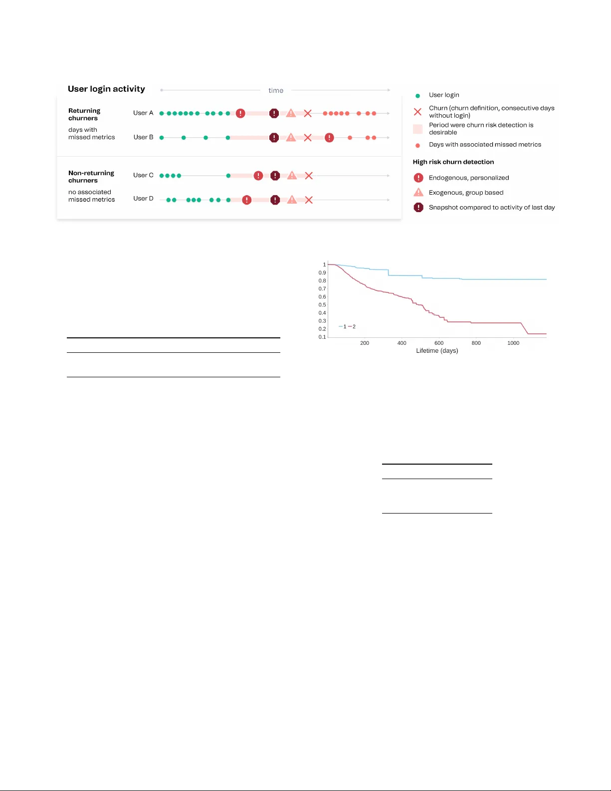
Leave a Comment