Master equation of discrete time graphon mean field games and teams

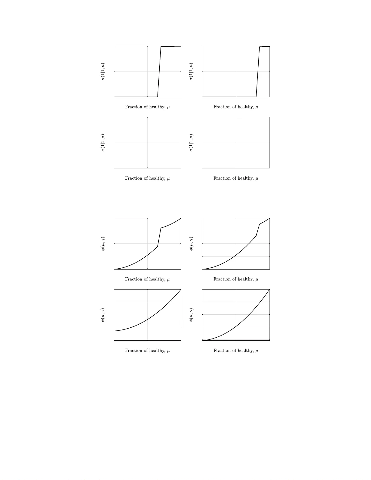
1 Master equation of discrete time graphon mean field games and tea ms Deepan s hu V asal, Raje s h Mishra and Sri ram V ishwanath Abstract In this paper , we present a sequential decomposition algorithm equiv alent of Master equation to compute graphon mean-field equillibrium (GMFE) of graphon mean-field ga mes (GM FGs) and g raphon optimal Mark ovian policies (GOMPs) of graphon mean field teams (GMFTs). W e consider a large population of players sequentially making strategic decisions where the actions of each player af fect their neighbors which is captured in a graph, generated by a kno wn graphon. Each player observ es a priv ate state and also a common information as a graphon mean-field population state which represents the empirical network ed distribution of oth er players’ types. W e consider non- stationary population state dynamics and present a nove l backward recursiv e algorithm to compute both GMFE and GOMP that depend on both, a player’ s priv ate type, and the current (dynamic) population state determined through the graphon . E ach step in computing GMFE consists of so lving a fixed-p oint equation, while compu ting GOMP in volves solving for an optimization prob lem. W e pro vide conditions on model parameters fo r which there exists such a GMFE. Using this algorithm, we obtain the GMFE and GOMP for a specific security setup in cyber physical systems for differen t graphons that capture the interactions between the nodes in the system. Index T erms Graphon mean-field teams and games, Sequential decompo sition, Signaling, Optimal Mark ov strategies I . I N T R O D U C T I O N Interaction of intercon nected agents has been an important topic of study f or many decades and its relev ance has been increa sin g rap idly wi th the p rogress of intern et pen etration an d smar tphone devices in o ur society . T he recent d ecade h a s seen tremen dous technolog ical advancement in th e field of networking ap plications th at h a s led to an un preceden ted scale o f interaction amon g pe ople a nd devices such as in ride sharin g platforms, social media apps, cyber-physical systems, auto nomou s vehicles and drones, large scale renew able en ergy , electric vehicles, cryptocu rrencies and smart grid systems. For instance, the in flu ence of social networks in the de c ision m aking of majority of individuals is a known ph enomeno n. Most decisions by in dividuals from which products to buy to whom to vote for ar e influenced by f r iends and acqu aintances. Th e emerging em pirical evidence on these issues motiv ate s the theoretical study of network effects with strategic a n d non strategic agen ts. Th e analysis, design and Deepanshu V asal is with Department of Electri cal and Compute r Engineering at Northwestern U nive rsity . Rajesh Mishra and Sriram V ishwanath are with Depart ment of Electrical and Computer Engineerin g at Uni versity of T exas, Austin. Part of the paper was presente d at [1]. 2 control of such systems that in volve such in teractions emb edded in a networked e nvironmen t could lead to m ore intelligent a n d efficient applica tio ns, and ca n enha nce our understand ing of the mechanic s of such interactio ns. Many of the ab ove men tioned application s of interest have fo llowing key features: (a) large n u mber of strategic or n on strategic play ers (b) dynam ically evolving incomp lete info rmation, and (c) an underly ing network. When the decision makers are non strategic, o ne can pose such pro blems as dece ntralized stochastic contro l problems on a network and in gen e ral such problem s are extremely hard (see [2], [3] and references th erein). When it comes to problem s with strategic interactio ns, game theor y is a natur al choice to mo del such inter actions where the pay offs obtained by individuals depen d on the action of her neig hbors. A shor tcoming of the stand ard app roach to solve dynamic network games with incomplete informa tio n is the inter depend e nce o f strategies of the play e rs across time. Moreover, as the nu mber of p layers becom e large as is the case in m any pr actical scenar ios considered here, computin g Nash equ ilibrium becomes intractable. A. Relevant Literatur e For th e decentralized team problems, W itsenh ausen p rovided a ‘simple’ two stage L QG system [2] where he showed tha t linear policies are no t o ptimal and to this day we don’t kn ow the op timal po licies fo r that sy stem showing h ow such simple lookin g de c entralized control system could be extremely hard. Decentralized contr ol systems have b een studied extensively in the literature where not too long ago Nayyar et al in [3] (see refer ences there in) presented a common agent a ppr oa ch where showed th at a class of decentralized co ntrol problem s with common inform ation ca n be posed as a sing le agent partially ob served Markov decision problems and thus in principle can be solved using d ynamic prog ramming. Arabneyd i and Mahajan p osed such a problem with large number of play ers as Mean field team problems in [4] and provided a dynamic pr ogramm in g appr o ach to find optimal M arkovian po licies for such pr oblems. There is a hug e literature o n stud ying dy namic decision pro b lems when th e users are strategic. Maskin and T iro le in [5] intro duced th e concept of Mar kov perfect equillibr ium ( M PE) for dynamic games governe d b y an under lying Markov decision p rocess (MDP). The strategies thus co mputed d epend on the present state and not on the past trajectory of the game . In g e neral, there exists a backward recur si ve m ethodolo gy to compu te MPE o f the game. Some pro minent examples of the ap plication of MPE in clude [6], [7], [ 8]. Ericso n and Pakes in [6] m odel ind ustry dynamics for firms’ entry , exit an d in vestmen t participation , throu g h a d ynamic g a m e with sym m etric in f ormation , compute its MPE, a n d p rove ergodicity of the equilibriu m process. Bergemann and V ¨ alim ¨ aki in [7] study a learnin g process in a dynamic oligop oly w ith strategic sellers and a single buyer , allowing for price co m petition among sellers. They study MPE of the g ame and its conv ergence behavior . Acemo ˘ glu and Robinson in [8] develop a theory o f p olitical transition s in a country by modelin g it as a repeate d game between th e elites a nd the poor, and study its MPE. When p layers ha ve pri vate t ypes then an ap p ropriate solution concept is perfect Bayesian equ ilibrium (PBE) an d sequen tial equilibir um ( SE). Recen tly au th ors in [9], [1 0], [11], [12], [13] presented backward recur si ve sequential decomposition method ologies to compute PBE for different classes of dynamic gam e s of incomplete informa tio n. 3 In large populatio n ga m es, compu ting MPE, PBE and SE with the methods spe c ified above become s intractable. Mean field game s (MFG) were intro duced in Huang, Malham ´ e,and Caines [14], and Lasry and Lion s [ 15] to model the strategic inter a ctions with large numbe r of players. In such game s, the individual agen ts have minimal impact of the overall outcome of the g ame an d so the agen ts tr a c k a mea n distribution of states o f other a g ents rath er than their actual states. MFGs is an excellen t and a tractable mod el to study large po pulation dy n amic game s of incomplete info rmation, a nd h as been shown to b e a go od a pproxim ation of Nash equ ilibrium (or MPE) of the original game as th e numbe r of play ers gr ow large (f or in stance see [ 16], [1 7], [18], [19], [20] an d referen ces therein). Parise and Ozdaglar in tr oduced th e notio n of grapho n games [2 1] to model large population static network games, wher e graphon is ge n erative model o f a large rando m graph inrodu ced b y Lov ¨ asz in [22]. Caines and Huang in [23] combine d the ideas of mean-field eq uillibrium (MFE) and graph o n g ames to define Grap hon Mean field ga m es ( GMFGs) wher e there a r e a large nu mber of strategic agen ts with d ynamic in c omplete inform ation who interact on an underly ing fixed network g e nerated by a k nown graphon . GMFGs com b ine the idea of n etwork games defined thr o ugh graphon s and the mean field framework of descr ib ing multi agent homo geneou s g ames and pred icting equilibrium in a tractable m anner . Large network of nodes interacting with one anoth er can be represented as graph ons and mean field ga mes deal with the stu d y o f such large inter a ction am ong d evices an d people as agents to analy z e such systems to d e sign and understan d the behavior o f such large scale interactions and their impact on our society . The progr ess in research in the mean field do main h av e be en re stricte d to cases where the ag ents inter acted in a perf ect homo g eneous en vironme nt and the interac tio ns between th e agents we re assume d to be unifo rm irrespective of the location of the agent in the network. Howe ver, in m any real world scenarios the populatio n in ter action is n ot unifo r m and there is a m easure o f how the agents intera cted with e ach o th er o r in other words, the pa yoff an d the transition to the next state is conditiona l on the r e la tive position of the agent in the network. T hen the mean field distribution would be affected b y it and so will the optimum policies and th e Nash equilibriu m thus gener ated. Th e the oretical basis for such a case has bee n p rovided in [2 3] which gener alizes the idea of me a n field g ames acro ss the populatio n with different levels of interaction s throu gh GM FG. In this pape r, we con sider both discou nted finite h orizon an d infinite-h orizon dynamic grapho n mean-field teams and gam e s where there is a large population of hom ogeneo u s p layers each having a priv ate type. Ea ch player sequentially makes decisions and is affected by oth er p la y ers in its neighbor hood th rough a graph on mean -field populatio n state. Each p layer has a private type tha t ev olves th rough a co ntrolled Markov process as a f unction of the gr a p hon, which only she observes an d all playe r s o bserve a comm on p opulation state which is the d istribution of o ther p la y ers’ typ es. In such ga m es, the graph on mean-field state ev o lves throug h McKean-Vlasov fo rward equation g iv en a po licy of the players an d the grapho n fu nction. Th e equilib r ium policy satisfies the Bellman backward equation, given the graphon mean-field states. Thus to c ompute equilibriu m, one needs to solve the coup led backward an d fo rward fixed-p oint e q uation in the grap h on mean -field and the eq uilibrium p olicy . W e prop ose a sequential decomposition algorith m to co mpute GMFEs and GOMPs by decompo sin g the problem acr o ss time. This alg o rithm is equiv alent to the Master eq uation of continu ous tim e mean field g ame [24] th at allows one to 4 compute all mean field equilibria ( M FE) of the game sequen tially . 1 In or der to demon strate the utility of our algorithm to compu te the GM FE and GOMP o f a graph on mean field game and a team for varying gra phons, we consider a cyber-security examp le of malware spr e ad pr oblem. A cluster of no des in a network o f phy sical servers get infec ted by an ind ependen t rand om proc e ss. For each nod e, there is a high er risk o f getting infected du e to negativ e externality imposed by other infec te d play ers. A grapho n functio n is defin ed that quantifies th e effect of th e effect of th e state of oth er nodes in the network on the c oncerned no d e. At each time t, a nod e pr ivately ob serves its own state a nd pub licly observes th e pop ulation o f infected n odes, based on wh ich it has to make a decision to repair or not. Upon takin g an action, the transition o f to th e next state is g overned by b oth its in dividual action and the actions affected b y the neighb oring ag ents given by a gr aphon function . Using o u r algorithm, we find eq uilibrium strategies of the p lay ers wh ich are o bserved to b e non- d ecreasing in the health y populatio n state. Similarly we fin d o ptimal Markovian policies for th e team prob lem. The p aper is structured as follows. In Section I I, we present a model of the graphon mean field game an d team, followed b y some preliminary result from ou r past research regarding MPE in strategic d ynamic games. In sectio n III, we pr esent our main results where we p r esent algo rithm to compu te MPE f or bo th finite and infinite hor izon game, a n d also present existence results. In Section IV we talk abou t th e existence o f GMFE. In Section V , we consider graphon team pro blem and provide a dyna m ic program to find optim al Markovian policies. In Section VI, we show the simulation results for the cyber-security exam p le assuming different graph ons an d conclud e in Section VII. B. Notatio n W e use upper case letter s f or ran d om variables and lowercase for their realization s. For any variable, subscrip ts represent time ind ices and sup erscripts r e present play er iden tities. W e use notation − α to represent a ll play ers othe r than player α i.e. − α = { 1 , 2 , . . . i − 1 , i + 1 , . . . , N } . W e use nota tio n a t : t ′ to re p resent th e vector ( a t , a t +1 , . . . a t ′ ) when t ′ ≥ t or an emp ty vector if t ′ < t . W e use a − α t to mean ( a 1 t , a 2 t , . . . , a i − 1 t , a i +1 t . . . , a N t ) . W e use the notation P x to r e p resent both P x and R x , an d the correct usage is deter m ined depen d ing o n the space of x . W e rem ove superscripts or subscrip ts if we want to represen t th e vector , for example a t represents ( a 1 t , . . . , a N t ) . W e denote the indicator fun ction of any set A by 1 { A } . For any finite set S , P ( S ) r epresents space of p robability measur es on S and |S | repre sen ts its card inality . W e den ote by P σ (or E σ ) th e prob ability measure generated by (or expectatio n with resp e ct to ) strategy p rofile σ . W e denote the set of real n umbers by R . For a probab ilistic strategy p rofile of players ( σ α t ) i ∈ [ N ] where probability o f action a α t condition ed o n µ G 1: t , x α 1: t is giv en by σ α t ( a α t | µ G 1: t , x α 1: t ) , we use the short hand n otation σ − α t ( a − α t | µ G 1: t , x − α 1: t ) to repre sen t Q j 6 = i σ j t ( a j t | µ G 1: t , x j 1: t ) . All equalities and inequalities in volving ran dom variables are to be interp reted in a.s. sen se. 1 Since the publishi ng an initi al version of this paper in [25], aut hors in [26] hav e computed a Master’ s equation for Linear Quadratic Gaussian (LQG) GMFG. 5 I I . M O D E L A N D B A C K G R O U N D A. Grapho n Mean F ield Gam e s and T ea ms Let us consid e r a d iscrete-time large popu lation sequen tial gam e with N homog eneous p layers with N → ∞ . The interac tions between these N players are ca ptured in a asympto tically infin ite network grap h r epresented as a graphon . Grapho ns are b ounde d sym metric L ebesgue me a su rable fun ctions W : [0 , 1] 2 → [0 , 1 ] which can be represented as weighted g r aphs o n the vertex set [0 , 1] such that G = { g ( α, β ) : 0 ≤ α, β ≤ 1 } [23]. I t is similar to an adjacency m a trix d e fined over a 2 - dimensiona l plan e wher e each en try in the matrix is th e measure of co upling between the agen ts concern ed. In each per iod t ∈ [ T ] , where [ T ] repre sents th e time horizon , a p layer α ∈ [0 , 1] observes a private ty pe x α t ∈ X and a co mmon ob ser vation µ G t , the n takes an action a α t ∈ A and rece ives a reward R ( x α t , a α t , µ G t ) . The co mmon observation is an ensemble of the mean field distributions with respect to all agents α ∈ [0 , 1] given as µ G t = { µ α t } α where µ α t ( x ) = P { x α t = x } (1) with P N x i =1 µ α t ( i ) = 1 . Player α ’ s type ev olves as a contro lled Markov process, x α t +1 = ˜ f [ x α t , a α t , µ G t ; g α ] + w α t . (2) The ra n dom variables ( w α t ) α,t are assumed to be mu tu ally indepen dent acro ss players and across time. W e also write the above upd ate of x α t throug h a kernel, x α t +1 ∼ Q α ( ·| x α t , a α t , µ G t ; g α ) which depen d s on the graph on func tio n g α = { g ( α, β ) : 0 ≤ β ≤ 1 } . The dyn a m ics of the MDP are g overne d both by the local inform ation as well as the g lobal d ynamics inv o lv ing the effect of the policy actio n o f oth er p layers in the system. T he id ea of gr aphon is to cap ture the effect of the actions of all the o ther play ers β ∈ [0 , 1 ] on pla y er α . In prio r mean field resear ch, it was assumed that there is a p erfect interaction between th e p layers and a lso tha t these interactions were un iform. In [23], they p rovide a set of differential equations that govern such interactio ns in the mean field setting. The fun ctions below show how the grapho n is u sed in d etermining th e effect of p layers on one another . T h e f unction ˜ f in (2) is g i ven as ˜ f [ x α t , a α t , µ G t ; g α ] = f 0 ( x α t , a α t ) + f  x α t , a α t , µ G t ; g α  (3) where f  x α t , a α t , µ G t ; g α  = Z β ∈ [0 , 1] X x β ∈X f  x α t , a α t , x β  g ( α, β ) µ β t ( x β ) d ( x β ) dβ (4) and f 0 represent the local effect o f th e agent when it takes any action and is ind ependen t o f th e actions taken by other agents. In th e case, when the agents do not interact a t all i.e . g ( α, β ) = 0 , the markov proce ss reduces o nly to the fun ction f 0 ignorin g the degener ate case when α = β . At instant t , the p layer α ob serves the trajec to ry ( µ G 1: t , x α 1: t ) and takes an actio n a α t accordin g to a behavioral strategy σ α = ( σ α t ) t , whe re σ α t : ( µ G ) t × X t → P ( A ) . W e denote th e space of suc h strategies as K σ . Th is imp lies A α t ∼ σ α t ( ·| µ G 1: t , x α 1: t ) . W e den ote Z t to be the space of populatio n states µ G 1: t till time t . W e den o te H α t = Z t × X t to be set of observed histories ( µ G 1: t , x α 1: t ) of p la y er α . 6 For fin ite time-h orizon g ame, G T , each player wants to maximize its total exp e c ted disco unted reward over a time horizon T , disco u nted by discount factor 0 < δ ≤ 1 , J α,T Game := E σ " T X t =1 δ t − 1 R ( X α t , A α t , µ G t ; g α ) # . (5) For the infinite time-horizo n game, G ∞ , each p la y er wants to m aximize its total expected d iscounted reward over an infin ite- time hor izon discoun ted by a discou nt factor 0 < δ < 1 , J α, ∞ Game := E σ " ∞ X t =1 δ t − 1 R ( X α t , A α t , µ G t ; g α ) # . (6) Similarly for finite time-ho rizon team , T T , all p layers wants to max im ize their average tota l expected d iscounted rew ard over a time ho rizon T , d isco unted by discoun t factor 0 < δ ≤ 1 , J T T eam := E σ   T X t =1 δ t − 1 X x α t µ α t ( x α t ) R ( x α t , A α t , µ G t ; g α )   . (7) For the infinite time -horizon team, T ∞ , each player wants to maximize its total expected discounted reward over an infin ite- time hor izon discoun ted by a discou nt factor 0 < δ < 1 , J ∞ T eam := E σ   ∞ X t =1 δ t − 1 X x α t µ α t ( x α t ) R ( x α t , A α t , µ G t ; g α )   . (8) B. So lution conc e pt: GMFE For grap hon mean field games, notion of equilibriu m is GMFE [5], which we u se in this pape r . A GM FE ( ˜ σ ) satisfies seq u ential ratio n ality such th a t fo r G T , ∀ α ∈ [0 , 1] , t ∈ [ T ] , µ G 1: t , x α 1: t , σ α , E ( ˜ σ α ˜ σ − α ) " T X n = t δ n − t R ( X α n , A α n , µ G n ; g α ) | µ G 1: t , x α 1: t # ≥ E ( σ α ˜ σ − α ) " T X n = t δ n − t R ( X α n , A α n , µ G n ; g α ) | µ G 1: t , x α 1: t # , (9) GMFE for G ∞ are defined in a similar way where summation in the above equ ations is ta ken such th at T is replaced by ∞ . C. S olution concep t: G raph on mean field tea m optimal For graph on mean field teams, we use the no tion of optimality a s follows. A po licy ( σ ∗ ) is team optimal if f or ∀ α ∈ [0 , 1 ] , t ∈ [ T ] , µ G 1: t , σ α , E σ ∗   T X n = t δ n − t X x α t µ α t ( x α n ) R ( x α n , A α n , µ G n ; g α ) | µ G 1: t   ≥ E σ   T X n = t δ n − t X x α t µ α t ( x α n ) R ( x α n , A α n , µ G n ; g α ) | µ G 1: t   , (10) The notion o f op timality for T T are d efined in a similar way where summation in th e above equ ations is taken such tha t T is replaced by ∞ . 7 I I I . A M E T H O D O L O G Y T O C O M P U T E G M F G S In this section , we will provide a backward recursive metho d ology to c o mpute GMFGs for both G T and G ∞ . W e will consider Markovian equilib rium strategies of playe r α wh ich d epend o n the common information at time t , µ G t , an d o n its current type x α t . 2 Equiv alently , player α takes a ction of th e form A α t ∼ σ α t ( ·| µ G t , x α t ) . Similar to the common agent app roach in [3], an alternate and equ ivalent way of defining th e strategies of the p layers is as follows. W e first g enerate partial fu nction γ α t : X → P ( A ) as a function of µ G t throug h an eq uilibrium gener ating fun ction θ α t : µ G → ( X → P ( A )) such th at γ α t = θ α t [ µ G t ] . T hen action A α t is generated b y app lying this prescription fun ction γ α t on p layer α ’ s curren t priv ate inform ation x α t , i. e . A α t ∼ γ α t ( ·| x α t ) . Th us A α t ∼ σ α t ( ·| µ G t , x α t ) = θ α t [ µ G t ]( ·| x α t ) . For a given pr escription func tion γ α t = θ α [ µ G t ] , the gr a phon mean - field µ G t ev olves acco rding to the discrete-time McKean Vlasov equation , ∀ y ∈ X and ∀ α ∈ [0 , 1] : µ α t +1 ( y ) = X x ∈X X a ∈A µ α t ( x ) γ α t ( a | x ) Q  y | x, a, µ G t ; g α  , (11) which im p lies µ α t +1 = φ ( µ α t , γ α t , µ G t ; g α ) (12) µ G t +1 = φ ( µ G t , γ t ; g α ) (13) A. Ba c kwar d r ecursive algo rithm for G T In this subsectio n, we will pr ovide a methodo logy to gener ate GMFE o f G T of the for m described ab ove. W e define an equilibr ium g enerating function ( θ t ) t ∈ [ T ] , where θ t : µ G → {X → P ( A ) } , where for each µ G t , we generate ˜ γ t = θ t [ µ G t ] . In addition, we generate a rew ar d -to-go fu nction ( V α t ) t ∈ [ T ] , where V α t : µ G × X → R . These quantities ar e gener ated throug h a fixed-po int equation as follows. 1) Initialize ∀ µ G T +1 , α, x α T +1 ∈ X , V α T +1 ( µ G T +1 , x α T +1 ) △ = 0 . (14) 2) F o r t = T , T − 1 , . . . 1 , ∀ µ G t , let θ t [ µ G t ] be g enerated as follows. Set ˜ γ t = ( ˜ γ α t ) α ∈ [0 , 1] = θ t [ µ G t ] , where ˜ γ t is the solution of the following fixed-point equation 3 , ∀ α ∈ [0 , 1] , x α t ∈ X , ˜ γ α t ( ·| x α t ) ∈ arg max γ α t ( ·| x α t ) E γ α t ( ·| x α t )  R ( X α t , A α t , µ G t ; g α ) + δV α t +1 ( φ ( µ G t , ˜ γ α t ; g α ) , X α t +1 ) | µ G t , x α t  , (15) where expectation in (15) is with respect to rand om variable ( A α t , X α t +1 ) th rough the probab ility measure γ t ( a α t | x α t ) Q α ( x α t +1 | x α t , a α t , µ G t ; g α ) . W e note th at the solu tion of (15), ˜ γ t , app ears b o th on the left of (15) and on the righ t side in the update o f µ G t , an d is thu s u nlike the fixed-po int equ ation found in Bayesian Nash equilibriu m . Furthermo re, u sing the quantity ˜ γ t found a bove, define ∀ α V α t ( µ G t , x α t ) △ = E ˜ γ α t ( ·| x α )  R ( X α t , A α t , µ G t ; g α ) + δV α t +1 ( φ ( µ G t , ˜ γ α t ) , X α t +1 ) | µ G t , x α t  . (16) 2 Note ho wev er , that the unilat eral dev iation s of the player are consid ered in the space of all strategie s. 3 W e discuss the existenc e of solutio n of this fixed-poi nt equation in Section IV 8 Then, an equ ilibrium strategy is defined as ˜ σ α t ( a α t | µ G 1: t , x α 1: t ) = ˜ γ α t ( a α t | x α t ) , (17) where ˜ γ t = θ [ µ G t ] . In the fo llowing theo rem, we show that the strategy thus constru cted is a GMFGs of th e ga m e. Theorem 1 . A strate gy ( ˜ σ ) constructed fr o m the ab ove algorithm is a n MPE o f the ga me i.e. ∀ t, h α t ∈ H α t , σ α , E ( ˜ σ α ˜ σ − α ) " T X n = t δ n − t R ( X α n , A α n , µ G n ; g α ) | µ G 1: t , x α 1: t # ≥ E ( σ α ˜ σ − α ) " T X n = t δ n − t R ( X α n , A α n , µ G n ; g α ) | µ G 1: t , x α 1: t # (18) Pr oof. Please see Appen dix A. B. Convers e In the fo llowing, we show that every GMFE can be fou nd using the ab ove back ward r e cursion. Theorem 2 (Converse) . Let ˜ σ b e a GMFE of the g raph on mean field g ame. Then th er e exists an equilibriu m generating function θ that satisfies ( 1 5) in backwar d r ecursion such tha t ˜ σ is defin e d using θ . Pr oof. Please see Appen dix C . C. Ba ckwar d r ecursive algo rithm for G ∞ In this section, we consider th e infinite-hor izon problem G ∞ , for which we assume the r eward fu nction R to be absolutely bo unded. W e define an equ ilibrium generating function θ : µ G → {X → P ( A ) } , where for each µ G t , we gen erate ˜ γ t = θ [ µ G t ] . In add ition, we gener ate a reward-to-go fu nction V : µ G × X → R . These qua n tities ar e generated throug h a fixed-po int equ ation as follows. For all µ G , set ˜ γ = θ [ µ G ] . T hen ( ˜ γ , V ) are solutio n of the fo llowing fixed-p oint eq uation 4 , ∀ µ G , x α ∈ X , ˜ γ α ( ·| x α ) ∈ arg max γ α ( ·| x α ) E γ α ( ·| x α ) h R ( x α , A α , µ G ; g α ) + δV α ( φ ( µ G , ˜ γ ; g α ) , X α ′ ; g α ) | µ G , x α i , (19) V α ( µ G , x α ) = E ˜ γ ( ·| x α ) h R ( x α , A α , µ G ; g α ) + δ V α ( φ ( µ G , ˜ γ ; g α ) , X α ′ ) | µ G , x α i . (20) where expectation in (1 9) is with respect to random variable ( A α , X α, ′ ) through the measure γ ( a α | x α ) Q α ( x α ′ | x α , a α , µ G ) . Then an equ ilibrium strategy is defined a s ˜ σ α ( a α t | µ G 1: t , x α 1: t ) = ˜ γ ( a α t | x α t ) , (2 1) where ˜ γ = θ [ µ G t ] . The fo llowing the o rem shows that th e strategy thu s co n structed is a GMFE of the g ame. 4 W e discuss the existenc e of solutio n of this fixed-poi nt equation in Section IV 9 Theorem 3 . A strate gy ( ˜ σ ) constructed fr o m the ab ove algorithm is a GMFE of the ga me i.e. ∀ t, h α t ∈ H α t , σ α , E ( ˜ σ α ˜ σ − α ) " ∞ X n = t δ n − t R ( X α n , A α n , µ G n ; g α ) | µ G 1: t , x α 1: t # ≥ E ( σ α ˜ σ − α ) " ∞ X n = t δ n − t R ( X α n , A α n , µ G n ; g α ) | µ G 1: t , x α 1: t # , (22) Pr oof. Please see Appen dix D. D. Conver se In the fo llowing, we show that every GMFE can be fou nd using the ab ove back ward r e cursion. Theorem 4 (Converse) . Let ˜ σ be a GMFE the graphon mean field game. Then ther e exists an eq u ilibrium generating function θ th at satisfies (15) in ba ckw ar d r ecursion such tha t ˜ σ is defin ed using θ . Pr oof. Please see Appen dix F . I V . E X I S T E N C E In this section, we discuss sufficient co n ditions fo r the existence of a so lution of the fixed-p o int equation s (15) and ( 19). Assumption 1 (A1) . Th e a ction set A is a compa ct set. Assumption 2 (A2) . ˜ f  x α t , a α t , µ G t ; g α  and R ( x α t , a α t , µ G t ; g α ) ar e Lipschitz con tin uous in x α t and un iformly continuo us with respect to a α t . Assumption 3 (A3) . The first a nd second derivatives of ˜ f  x α t , a α t , µ G t ; g α  and R ( x α t , a α t , µ G t ; g α ) with r espect to x α t ar e continu ous and bound ed. Assumption 4 (A4 ) . ˜ f  x α t , a α t , µ G t ; g α  ar e Lipschitz co ntinuou s in a α t and u niformly contin uous with respect to x α t . Assumption 5 (A5) . F or a ny v ∈ R , α ∈ [0 , 1] and any pr oba bility measur e en semble µ G , th e set S ( x α t , v ) = ar g min a α t [ v  ˜ f  x α t , a α t , µ G t ; g α   + R ( x α t , a α t , µ G t ; g α )] (23) is a singleton and the r esulting a α t as a fu nction of ( x α t , v ) is Lip schitz c o ntinuou s in ( x α t , v ) and unifo rm with r espect to µ G t and g α . Theorem 5. Un der assumption s ( A 1)-(A5 ) , ther e exists a solution of th e fixed-p oint eq uations (15) a n d (1 9) for every t . Pr oof. Under the assumption (A1)-(A5) , it has been shown in [23] tha t th ere exists a solutio n to the GM FG equations. Conc u rrently , Th e o rem 2 and Th eorem 4 show that all GMFE can be fou nd u sing backward recu rsion 10 for the finite an d infinite horizo n pro blems. This proves that u nder (A1)- (A5), there exists a solu tion of (15) and (19) at every t . V . M E T H O D O L O G Y T O C O M P U T E G R A P H O N M E A N FI E L D T E A M O P T I M A L P O L I C I E S In this section , we will p rovide a c ommon agent based back ward recursive dyn amic pro gramming meth odolog y to compute optimal policies for both T T and T ∞ . As in Section III, we will consider Mar kovian eq u ilibrium strategies of playe r α which de p end on the co mmon info rmation at time t , µ G t , and on its curr ent typ e x α t . Equivalently , player α takes actio n of the fo rm A α t ∼ σ α t ( ·| µ G t , x α t ) . As befor e, we first generate p artial function γ α t : X → P ( A ) as a f unction of µ G t throug h an equilibrium generating f unction θ α t : µ G → ( X → P ( A )) such that γ α t = θ α t [ µ G t ] . Then action A α t is g enerated b y apply ing this prescription func tio n γ α t on play er α ’ s cur rent p riv ate info r mation x α t , i. e . A α t ∼ γ α t ( ·| x α t ) . Thus A α t ∼ σ α t ( ·| µ G t , x α t ) = θ α t [ µ G t ]( ·| x α t ) . A. Ba c kwar d r ecursive algo rithm for T T In this subsectio n, we will provide a dynamic program m ing meth odolog y to generate team optimal strategies of T T of the form d escribed above. W e d efine an optimal gen erating fun ction ( θ t ) t ∈ [ T ] , where θ t : µ G → {X → P ( A ) } , where for each µ G t , we gene r ate γ ∗ t = θ t [ µ G t ] . In addition , we g enerate a r e ward-to-go fu nction ( V t ) t ∈ [ T ] , where V t : µ G t → R . These quantities ar e gener ated throug h a back ward recursive optimiza tio n equation as follows. 1) Initialize ∀ µ G T +1 , V T +1 ( µ G T +1 ) △ = 0 . (24) 2) F o r t = T , T − 1 , . . . 1 , ∀ µ G t , let θ t [ µ G t ] be generated as follows. Set γ ∗ t = θ t [ µ G t ] , wh ere γ ∗ t is the solution of the fo llowing op timization equation, γ ∗ t ∈ a rg max γ t E γ t   X α ∈ [0 , 1] X x α t µ α t ( x α t ) R ( x α t , A α t , µ G t ; g α ) + δV t +1 ( φ ( µ G t , γ t ; g α )) | µ G t   , (25) where expectatio n in (15) is with re sp ect to r andom variable A α t throug h the prob ability measure γ α t ( a α t | x α t ) . Furthermo re, u sing the quantity γ ∗ t found a bove, d efine V t ( µ G t ) △ = E ˜ γ α t ( ·| x α )   X α ∈ [0 , 1] X x α t µ α t ( x α t ) R ( x α t , A α t , µ G t ; g α ) + δV t +1 ( φ ( µ G t , γ ∗ t ; g α )) | µ G t   . (26) Then, the op timal Markovian strategy is defined as σ ∗ ,α t ( a α t | µ G 1: t , x α 1: t ) = γ ∗ ,α t ( a α t | x α t ) , (27) where γ ∗ t = θ [ µ G t ] . In th e fo llowing theorem , we show th at the strategy th us con structed is a n op timal Mar kovian strategy of the team pr oblem. 11 Theorem 6. A strate gy ( σ ∗ ) constructed fr om the a bove a lgorithm is an optimal Ma rkovian strate gy of the team pr oblem i.e. ∀ t, µ G 1: t , σ α , E σ ∗   T X n = t δ n − t X α ∈ [0 , 1] X x α t µ α t ( x α t ) R ( x α n , A α n , µ G n ; g α ) | µ G 1: t   ≥ E σ   T X n = t δ n − t X α ∈ [0 , 1] X x α t µ α t ( x α t ) R ( x α n , A α n , µ G n ; g α ) | µ G 1: t   (28) Pr oof. It is easy to see th at { µ G t , γ t } t is a controlled Markov proc e ss for this p roblem since µ G t +1 = φ ( µ G t , γ t ) and the curr ent rewards can be written as a functio n of µ G t , γ t . Thus the result is a standar d applicatio n Markov decision th eory [27]. B. Ba c kwar d r ecursive algo rithm for T ∞ In this section , we co nsider the infinite-ho rizon prob lem T ∞ , for which we assume th e rew ar d f u nction R to b e absolutely bo unded. W e define an optimal gen erating functio n θ : µ G → {X → P ( A ) } , where for each µ G t , we g enerate γ ∗ t = θ [ µ G t ] . In add ition, we gener a te a reward-to-go fu nction V : µ G → R . These qu antities are gen erated through a fixed-p oint equation as follows. For all µ G , set γ ∗ = θ [ µ G ] . T hen ( γ ∗ , V ) ar e solution of the f ollowing fixed- point equation, ∀ µ G , γ ∗ ∈ a rg max γ E γ   X α ∈ [0 , 1] X x α µ α t ( x α ) R ( x α , A α , µ G ; g α ) + δV ( φ ( µ G , γ ∗ ; g α ) | µ G   , (29) V ( µ G ) = E ˜ γ ( ·| x α )   X α ∈ [0 , 1] X x α t µ α t ( x α t ) R ( x α , A α , µ G ; g α ) + δV ( φ ( µ G , γ ∗ ; g α )) | µ G   . (30) where expe c tation in (1 9) is with respect to rando m variable ( A α ) throug h the mea sure γ ( a α | x α ) . Then the optim al Markovian strategy is defined a s σ ∗ ,α t ( a α t | µ G 1: t , x α 1: t ) = γ ∗ ,α t ( a α t | x α t ) , (31) where γ ∗ t = φ [ µ G t ] . The following theor em shows that the strategy thus co nstructed is a n op timal Markovian policy of the team problem . Theorem 7. A strate g y ( σ ∗ ) constructed fr o m the above algorithm is an o ptimal Markovian policy of the tea m pr oblem i.e. ∀ t, µ G 1: t , σ α , E σ ∗   ∞ X n = t δ n − t X α ∈ [0 , 1] X x α t µ α t ( x α t ) R ( x α n , A α n , µ G n ; g α ) | µ G 1: t   ≥ E σ   ∞ X n = t δ n − t X α ∈ [0 , 1] X x α t µ α t ( x α t ) R ( x α n , A α n , µ G n ; g α ) | µ G 1: t   , (32) 12 Pr oof. By sam e argument as proof of Theor e m 6, since { µ G t , γ t } t is a contro lled Markov proc e ss for this problem as µ G t +1 = φ ( µ G t , γ t ) a nd the cu rrent rewards can be written as a fu nction of µ G t , γ t . Also R is a bsolutely boun ded. Therefo re, th e resu lt is a standar d app lication Markov decision theo ry [2 7]. V I . N U M E R I C A L E X A M P L E In th is section, we put forth a nu merical examp le to showcase the pro posed sequ e n tial decomp osition in the context of a system where the relative p osition of the players with respect to other players in a grap h affects the state of the player as we ll as their e q uilibrium strategies. W e provid e the following definition . Definition 1 . Players α an d β ar e statistically equivalen t if φ α ( µ, γ , µ G ; g α ) = φ β ( µ, γ , µ G ; g β ) . Proposition 1. Mean fie ld games with sta tistically equ ivalent players share the same mean fi eld distribution and µ G can b e r eplaced by µ α for a ll α ∈ [0 , 1] . For a com plete, E rdos R ´ enyi, symm e tric stoch a stic block mo del, and rando m geom e tric graph on, every player is statistically eq uiv alen t. Thu s from prop osition 1, the players share the same McKean-Vlasov (MKV) mean field ev olu tion function and so the same mean field . Let n be th e total n umber of statistically different pla y ers. Th en µ G can be r e placed by { µ } i =1 ,...,n . W ith the propo sition we can represent the gr aphon mean field populatio n state as µ G = { µ } i =1 ,...,n = µ ∀ i (33) A. Cybersecurity Example W e consider a cyber-security examp le where a c lu ster o f n odes, facing a possible malware attack in a network, do a cost-benefit analysis to d etermine wh e ther to o pt f o r re p airing. T he re su lts of this analysis, however , could be extended to many different cases like the vaccination in a popu lation, entr y and exit of firms, fin ancial markets, demand respo nse in smart-gr id and so on. The dy namics of each of the nod e is affected by the action of the neighbo ring n o des conn e cted with different measures ca p tured in a network graph an d represen ted as a grap hon function G . In this example, we assum e different grapho n fu nctions and obta in the optimal policie s u sin g our sequential decompo sition alg orithm assum ing that the graph s are symmetric with respec t to the participating a g ents. In the mod el, th e node can have two states x α ∈ X = { 0 , 1 } represen ting health y and inf ected node respectively . Similarly , there are two actio n s at their disposal f or ea ch of the state a α ∈ A = { 0 , 1 } which says whether the nodes gets repa ired with a cost or takes the r isk by not undergoing repair . The chances o f a nod e getting affected by a malware attack depend s on the population as well as the state o f the neighbo ring no des according to the grap hon. The d y namics of the m odel ar e given as x α t +1 =    x α t + (1 − x α t ) w α t if a α t = 0 0 otherwise (34) where w α t ∈ { 0 , 1 } is a binary r andom variable with P { w α t = 1 } = Z β ∈ [0 , 1] X x β ∈X f  x α t , a α t , x β  g ( α, β ) µ β t ( x β ) d ( x β ) dβ (35) 13 It is assumed that the value o f P { w α t = 1 } is q w h en the graph is fully con nected i.e. g ( α, η ) = 1 an d the me an state of the neig hbors µ t ( x β ) = 1 . The value of q is a ssumed to be 0 . 9 f o r ou r game an d 0 . 4 fo r th e team simulation s. The reward fun ction is g i ven as r ( x α t , a α t , µ t ) = − k x α t − λa α t (36) The value k represents the penalty if the node g ets infected and λ repr esents th e cost of repair . Th e values k and λ are assumed as 0 . 3 and 0 . 2 r e spectiv ely fo r our simulation. Here we implement ou r algorithm to derive equ ilibrium for this p r oblem b y co n sidering th ree p opular n etwork m o dels to capture the in te r action betwee n the popu la tio n. W e consider the following grapho ns: 1) Fully Connected Graph : The g r aphon func tion is given as g ( α, β ) = 1 ∀ α, β (37) 2) Er d ¨ os Renyi Graph : The graph on f unction is given as g ( α, β ) = p ∀ α, β (38) W e assume a value p = 0 . 8 fo r our simulation. 3) Stochastic Blo ck Mo del : The graph on f unction is given as g ( α, β ) =    p if α, β ≤ 0 . 5 or α, β ≥ 0 . 5 q otherwise (39) Here, p rep resents the intr a -commun ity in teraction and is assum ed as p = . 9 for o ur simulation. Similar ly , q = . 4 rep resents the inter-community interaction p arameter . 4) Random Geometric g raph : The grapho n fu nction is giv en as g ( α, β ) = f (min( β − α, 1 − β + α )) (40) where f : [0 , . 5] → [0 , 1] is a non- in creasing function , and in our simu lation we assum e it to be f ( x ) = e x 0 . 5 − x . Figure VI- A shows the eq uilibrium policy d eriv ed for different grap hons for th e specific cyber-security examp le. The policies differ a s the interactio n of the ag e n ts with their neighbo rs influences their strategies. Figure VI-A gives the relation between µ t and µ t +1 as presented in th e (11). Fig u re VI -A shows the equilibrium me an field o r in the specific case that we c onsider when with time, the a mea n field distribution of 0 . 5 ap proache s d ifferent mean field states for different grap h ons but with the sam e state dynamics. In Figu res VI-A, VI-A, V I -A, we plot the policies and mea n field equilib rium or different grapho ns for the specific cyber-security example when th e agents coo perate as a team. V I I . C O N C L U S I O N In this pap er , we consider both finite and infinite ho rizon, large population dynamic game (with individual re wards) and team(with comm on rew ar ds) wh ere each player is affected by oth ers throug h a grap hon m ean-field populatio n state. W e presen t a novel backward r ecursive alg orithm to co m pute non-stationar y , signaling GMFG and GOMP for such games, where each player ’ s strategy depend s on its curr ent private ty pe an d th e cur rent grapho n mean-field 14 0 0.5 1 0 0.5 1 Fully Connected Graph 0 0.5 1 0 0.5 1 Erdos-Renyi Graph 0 0.5 1 0 0.5 1 Statistical Block Graph 0 0.5 1 0 0.5 1 Random Geometric Graph Figure 1. Policy action at higher state for all graphons for the game 0 0.5 1 0 0.5 1 Fully Connected Graph 0 0.5 1 0.2 0.4 0.6 0.8 1 Erdos-Renyi Graph 0 0.5 1 0.2 0.4 0.6 0.8 1 Statistical Block Graph 0 0.5 1 0.6 0.7 0.8 0.9 1 Random Geometric Graph Figure 2. Mean Field Evolutio n at differe nt mean fields for the game problem populatio n state. T he non-tr i viality in th e problem is tha t th e u pdate of pop ulation state is coupled to the strategies of the game , and is manag ed in the algorithm through uniqu e con struction of the fixed-point eq uations (15),(19) f or GMFE an d through an optimization pr oblem (25) fo r the team problem. W e proved the existence of the fixed-poin t equations (15) under certain cond itions. Using this algor ithm, we co nsidered a malware pro pagation pro blem wher e 15 0 50 100 0 0.1 0.2 0.3 Fully Connected Graph 0 50 100 0.25 0.3 0.35 0.4 0.45 Erdos-Renyi Graph 0 50 100 0.54 0.56 0.58 0.6 Statistical Block Graph 0 50 100 0.7 0.8 0.9 1 Random Geometric Graph Figure 3. Con vergenc e to GMFGs for all graphons with time for the game problem 0 0.5 1 0 0.2 0.4 0.6 0.8 1 Fully Connected Graph 0 0.5 1 0 0.2 0.4 0.6 0.8 1 Erdos-Renyi Graph 0 0.5 1 0 0.2 0.4 0.6 0.8 1 Statistical Block Graph 0 0.5 1 0 0.2 0.4 0.6 0.8 1 Random Geometric Graph Figure 4. Policy action at higher state for all graphons for the team problem we nu merically comp u ted equilibrium an d team optimal strategies of the play ers. In g eneral, this algorithm be could instrumental in studying non-station ary equilibria and o p timal contro l in a num ber of applications such as finan cial markets, social learnin g, r e n ew a b le energy and more. 16 0 0.5 1 -0.8 -0.6 -0.4 -0.2 0 Fully Connected Graph 0 0.5 1 -0.8 -0.6 -0.4 -0.2 0 Erdos-Renyi Graph 0 0.5 1 -0.6 -0.4 -0.2 0 Statistical Block Graph 0 0.5 1 -1 -0.8 -0.6 -0.4 -0.2 0 Random Geometric Graph Figure 5. Mean Field Evolutio n at differe nt mean fields for the team proble m 0 50 100 0 0.5 1 1.5 2 Fully Connected Graph 0 50 100 0.9 0.92 0.94 0.96 0.98 1 Erdos-Renyi Graph 0 50 100 0.9 0.92 0.94 0.96 0.98 1 Statistical Block Graph 0 50 100 0.94 0.96 0.98 1 Random Geometric Graph Figure 6. Con vergenc e to GMFGs for all graphons with time for the team problem A P P E N D I X A Pr oof. W e prove (28) using induction and the resu lts in L emma 1 , an d 2 proved in A p pendix B. For base case at t = T , ∀ ( µ G 1: T , x α 1: T ) ∈ H α T , σ α E ˜ σ α T ˜ σ − α T  R ( X α t , A α t , µ G t ; g α )   µ G 1: T , x α 1: T  = V α T ( µ G T , x α T ) (41a) ≥ E σ α T ˜ σ − α T  R ( X α t , A α t , µ G t ; g α )   µ G 1: T , x α 1: T  , (41b) 17 where ( 41a) follows from Lemma 2 and (41 b) follows from Lem m a 1 in Ap pendix B. Let th e indu ction hypo thesis b e that for t + 1 , ∀ i ∈ [ N ] , µ G 1: t +1 ∈ ( H c t +1 ) , x α 1: t +1 ∈ ( X ) t +1 , σ α , E ˜ σ α t +1: T ˜ σ − α t +1: T ( T X n = t +1 δ n − t − 1 R ( X α n , A α n , µ G n ; g α )   µ G 1: t +1 , x α 1: t +1 ) (42a) ≥ E σ α t +1: T ˜ σ − α t +1: T ( T X n = t +1 δ n − t − 1 R ( X α n , A α n , µ G n ; g α )   µ G 1: t +1 , x α 1: t +1 ) . (42b) Then ∀ i ∈ [ N ] , ( µ G 1: t , x α 1: t ) ∈ H α t , σ α , we have E ˜ σ α t : T ˜ σ − α t : T ( T X n = t δ n − t − 1 R ( X α n , A α n , µ G n ; g α )   µ G 1: t , x α 1: t ) = V t ( µ G t , x α t ) (43a) ≥ E σ α t ˜ σ − α t  R ( X α t , A α t , µ G t ; g α ) + δ V α t +1 ( µ G t +1 , X α t +1 )   µ G 1: t , x α 1: t  (43b) = E σ α t ˜ σ − α t  R ( X α t , A α t , µ G t ; g α )+ δ E ˜ σ α t +1: T ˜ σ − α t +1: T ( T X n = t +1 δ n − t − 1 R ( X α n , A α n , µ G n ; g α )   µ G 1: t , µ G t +1 , x α 1: t , X α t +1 )   µ G 1: t , x α 1: t ) (43c) ≥ E σ α t ˜ σ − α t  R ( X α t , A α t , µ G t ; g α )+ δ E σ α t +1: T ˜ σ − α t +1: T ( T X n = t +1 δ n − t − 1 R ( X α n , A α n , µ G n ; g α )   µ G 1: t , µ G t +1 , x α 1: t , X α t +1 )   µ G 1: t , x α 1: t ) (43d) = E σ α t ˜ σ − α t  R ( X α t , A α t , µ G t ; g α )+ δ E σ α t : T ˜ σ − α t : T ( T X n = t +1 δ n − t − 1 R ( X α n , A α n , µ G n ; g α )   µ G 1: t , µ G t +1 , x α 1: t , X α t +1 )   µ G 1: t , x α 1: t  (43e) = E σ α t : T ˜ σ − α t : T ( T X n = t δ n − t R ( X α n , A α n , µ G n ; g α )   µ G 1: t , x α 1: t ) , (43f) where (4 3a) follows from L e mma 2, (43b) f ollows from Lemma 1, (43 c) follows fr om Lemm a 2, ( 43d) follows from induction hypo thesis in (42b) and (4 3e) fo llows since the rando m variables inv olved in the right conditio n al expectation do not d epend on strategies σ α t . A P P E N D I X B Lemma 1. ∀ t ∈ [ T ] , i ∈ [ N ] , ( µ G 1: t , x α 1: t ) ∈ H α t , σ α t V α t ( µ G t , x α t ) ≥ E σ α t ˜ σ − α t  R ( X α t , A α t , µ G t ; g α ) + δV α t +1 ( µ G t +1 , X α t +1 )   µ G 1: t , x α 1: t  . (44) Pr oof. W e prove this lemma b y contr adiction. Suppose the claim is not tru e for t . This im plies ∃ i, b σ α t , b µ G 1: t , b x α 1: t such tha t E b σ α t ˜ σ − α t  R ( X α t , A α t , µ G t ; g α ) + δV α t +1 ( µ G t +1 , X α t +1 )   b µ G 1: t , b x α 1: t  > V t ( b µ G t , b x α t ) . (45) W e will show that this leads to a contrad iction. Construct b γ α t ( a α t | x α t ) =    b σ α t ( a α t | b µ G 1: t , b x α 1: t ) x α t = b x α t arbitrary otherwise. (46) 18 Then for b µ G 1: t , b x α 1: t , we have V α t ( b µ G t , b x α t ) = max γ t ( ·| b x α t ) E γ t ( ·| b x α t ) ˜ σ − α t  R ( b x α t , A α t , b µ G t ) + δ V α t +1 ( φ ( b µ G t , ˜ γ t ; g α ) , X α t +1 )   b µ G t , b x α t  , (47a) ≥ E b γ α t ( ·| b x α t ) ˜ σ − α t  R ( X α t , A α t , µ G t ; g α ) + δV α t +1 ( φ ( b µ G t , ˜ γ t ; g α ) , X α t +1 )   b µ G t , b x α t  (47b) = X a α t ,x α t +1  R ( b x α t , a α t , b µ G t ) + δV t +1 ( φ ( b µ G t , ˜ γ t ; g α ) , x α t +1 )  b γ t ( a α t | b x α t ) Q α ( x α t +1 | b x α t , a α t , b µ G t ; g α ) = X a α t ,x α t +1  R ( b x α t , a α t , b µ G t ) + δV α t +1 ( φ ( b µ G t , ˜ γ t ; g α ) , x α t +1 )  b σ t ( a α t | b µ G 1: t , b x α 1: t ) Q α ( x α t +1 | b x α t , a α t , b µ G t ; g α ) = E b σ α t ˜ σ − α t  R ( b x α t , a α t , b µ G t ) + δV α t +1 ( φ ( b µ G t , ˜ γ t ) , X α t +1 ; g α )   b µ G 1: t , b x α 1: t  (47c) > V α t ( b µ G t , b x α t ) , (47d) where (4 7a) follows from definition of V t in (16), ( 47c) follows from definition o f b γ α t and (4 7d) follows from (45). Howe ver this leads to a contr adiction. Lemma 2. ∀ i ∈ [ N ] , t ∈ [ T ] , ( µ G 1: t , x α 1: t ) ∈ H α t , V α t ( µ G t , x α t ) = E ˜ σ α t : T ˜ σ − α t : T ( T X n = t δ n − t R ( X α n , A α n , µ G n ; g α )   µ G 1: t , x α 1: t ) . (48) Pr oof. W e prove the lem ma by ind uction. For t = T , E ˜ σ α T ˜ σ − α T  R ( X α t , A α t , µ G t ; g α )   V α ertµ G 1: T , x α 1: T  = X a α T R ( X α t , A α t , µ G t ; g α ) ˜ σ α T ( a α T | µ G T , x α T ) (49a) = V α T ( µ G T , x α T ) , (49b) where (4 9 b) f ollows from the definition of V α t in (1 6). Suppose the claim is true fo r t + 1 , i.e., ∀ i ∈ [ N ] , t ∈ [ T ] , ( µ G 1: t +1 , x α 1: t +1 ) ∈ H α t +1 V α t +1 ( µ G t +1 , x α t +1 ) = E ˜ σ α t +1: T σ − α t +1: T ( T X n = t +1 δ n − t − 1 R ( X α n , A α n , µ G n ; g α )   µ G 1: t +1 , x α 1: t +1 ) . (50) 19 Then ∀ i ∈ [ N ] , t ∈ [ T ] , ( µ G 1: t , x α 1: t ) ∈ H α t , we have E ˜ σ α t : T ˜ σ − α t : T ( T X n = t δ n − t R ( X α n , A α n , µ G n ; g α )   µ G 1: t , x α 1: t ) = E ˜ σ α t : T ˜ σ − α t : T  R ( X α t , A α t , µ G t ; g α ) + δ E ˜ σ α t : T ˜ σ − α t : T ( T X n = t +1 δ n − t − 1 R ( X α n , A α n , µ G n ; g α )   µ G 1: t , µ G t +1 , x α 1: t , X α t +1 )   µ G 1: t , x α 1: t ) (51a) = E ˜ σ α t : T ˜ σ − α t : T  R ( X α t , A α t , µ G t ; g α ) + δ E ˜ σ α t +1: T ˜ σ − α t +1: T ( T X n = t +1 δ n − t − 1 R ( X α n , A α n , µ G n ; g α )   µ G 1: t , µ G t +1 , x α 1: t , X α t +1 )   µ G 1: t , x α 1: t ) (51b) = E ˜ σ α t : T ˜ σ − α t : T  R ( X α t , A α t , µ G t ; g α ) + δV α t +1 ( µ G t +1 , X α t +1 )   µ G 1: t , x α 1: t  (51c) = E ˜ σ α T ˜ σ − α T  R ( X α t , A α t , µ G t ; g α ) + δV α t +1 ( µ G t +1 , X α t +1 )   µ G 1: t , x α 1: t  (51d) = V α t ( µ G t , x α t ) , (51e) (51c) f o llows f rom the inductio n hypo thesis in ( 50), (5 1 d) follows becau se the ran dom variables inv o lved in expectation, X α t , A α t , µ G t , µ G t +1 , X α t +1 do n ot dep end on ˜ σ α t +1: T σ − α t +1: T and (51 e) fo llows f rom the definition o f V α t in (16). A P P E N D I X C Pr oof. W e prove this by co ntradiction . Suppo se for any equilibr ium gen erating function θ tha t generates an MPE ˜ σ , there exists t ∈ [ T ] , i ∈ [ N ] , µ G 1: t ∈ H c t , such that (15) is n ot satisfied for θ i.e. for ˜ γ t = θ t [ µ G t ] = ˜ σ t ( ·| µ G t , · ) , ˜ γ t ( ·| x α t ) 6∈ arg max γ t ( ·| x α t ) E γ t ( ·| x α t )  R t ( X α t , A α t , µ G t ; g α ) + V α t +1 ( φ ( µ G t , ˜ γ t ; g α ) , X α t +1 )   x α t , µ G t  . (52) Let t be the first in stance in the b ackward recursion when th is hap p ens. This implies ∃ b γ t such tha t E b γ t ( ·| x α t )  R t ( X α t , A α t , µ G t ; g α ) + V t +1 ( φ ( µ G t , ˜ γ t ; g α ) , X α t +1 )   µ G 1: t , x α 1: t  > E ˜ γ t ( ·| x α t )  R t ( X α t , A α t , µ G t ; g α ) + V α t +1 ( φ ( µ G t , ˜ γ t ; g α ) , X α t +1 )   µ G 1: t , x α 1: t  (53) 20 This implies for b σ t ( ·| µ G t , · ) = b γ t , E ˜ σ t : T ( T X n = t R n ( X α n , A α n , µ G n ; g α )   µ G 1: t − 1 , x α 1: t ) (54) = E ˜ σ α t , ˜ σ − α t ( R t ( X α t , A α t , µ G t ; g α ) + E ˜ σ α t +1: T ˜ σ − α t +1: T ( T X n = t +1 R n ( X α n , A α n , µ G n ; g α )   µ G 1: t − 1 , µ G t +1 , x α 1: t , X α t +1 )   µ G 1: t , x α 1: t ) (55) = E ˜ γ t ( ·| x t ) ˜ γ − α t  R t ( X α t , A α t , µ G t ; g α ) + V α t +1 ( φ ( µ G t , ˜ γ t ; g α ) , X α t +1 )   µ G t , x α t  (56) < E b σ t ( ·| µ G t ,x α t ) ˜ γ − α t  R t ( X α t , A α t , µ G t ; g α ) + V α t +1 ( φ ( µ G t , ˜ γ t ; g α ) , X α t +1 )   µ G t , x t  (57) = E b σ t ˜ σ − α t ( R t ( X α t , A α t , µ G t ; g α ) + E ˜ σ α t +1: T ˜ σ − α t +1: T ( T X n = t +1 R n ( X α n , A α n , µ G n ; g α )   µ G 1: t , µ G t +1 , x α 1: t , X α t +1 )   µ G 1: t , x α 1: t ) (58) = E b σ t , ˜ σ α t +1: T ˜ σ − α t : T ( T X n = t R n ( X α n , A α n , µ G n ; g α )   µ G 1: t , x α 1: t ) , (59) where ( 79) f ollows from the definitions o f ˜ γ t and L e mma 2, (8 0) fo llows f rom ( 76) an d the definitio n of b σ t , (81) follows from Lemm a 1. Howe ver, this leads to a contrad iction sinc e ˜ σ is an MPE of th e ga m e. A P P E N D I X D W e d i vide the proof into two pa rts: first we show that th e value function V is at least as big as any reward-to-go function ; seco ndly we show that under the strategy ˜ σ , reward-to-go is V α . No te th at h α t := ( µ G 1: t , x α 1: t ) . P art 1 : For a ny i ∈ [ N ] , σ α define the following reward-to-go fu nctions W σ α t ( h α t ) = E σ α , ˜ σ − α ( ∞ X n = t δ n − t R ( X α n , A α n , µ G n ; g α ) | h α t ) (60a) W σ α ,T t ( h α t ) = E σ α , ˜ σ − α ( T X n = t δ n − t R ( X α n , A α n , µ G n ; g α ) + δ T +1 − t V α ( µ G T +1 , X α T +1 ) | h α t ) . (60b) Since X , A ar e fin ite sets the reward R is absolutely bound ed, the reward-to-go W σ α t ( h α t ) is finite ∀ i, t, σ α , h α t . For any i ∈ [ N ] , h α t ∈ H α t , V α  µ G t , x α t  − W σ α t ( h α t ) = h V α  µ G t , x α t  − W σ α ,T t ( h α t ) i + h W σ α ,T t ( h α t ) − W σ α t ( h α t ) i (61) Combining r esults from Lemmas 4 and 5 in Ap pendix D, th e ter m in the first bra cket in RHS of (61) is non- negati ve. Using (6 0), the term in th e second bracket is  δ T +1 − t  E σ α , ˜ σ − α n − ∞ X n = T +1 δ n − ( T +1) R ( X α n , A α n , µ G n ; g α ) + V α ( µ G T +1 , X α T +1 ) | h α t o . (62) The summation in the expression ab ove is bound ed by a conver gent geometric ser ies. Also, V α is boun ded. Hence the ab ove q uantity can be mad e arb itrarily small by choo sing T approp riately large. Since the LHS of (61) does not d e p end on T , which implies, V α  µ G t , x α t  ≥ W σ α t ( h α t ) . (63) 21 P art 2: Since th e strategy the equilibr ium strategy ˜ σ genera te d in (31) is such that ˜ σ α t depend s on h α t only throug h µ G t and x α t , th e reward-to-go W ˜ σ α t , at strategy ˜ σ , can be written (w ith abuse of notation ) as W ˜ σ α t ( h α t ) = W ˜ σ α t ( µ G t , x α t ) = E ˜ σ ( ∞ X n = t δ n − t R ( X α n , A α n , µ G n ; g α ) | µ G t , x α t ) . (64) For any h α t ∈ H α t , W ˜ σ α t ( µ G t , x α t ) = E ˜ σ n R ( X α t , A α t , µ G t ; g α ) + δW ˜ σ α t +1  φ ( µ G t , θ [ µ G t ] , g α )) , X α t +1  | µ G t , x α t o (65a) V α ( µ G t , x α t ) = E ˜ σ n R ( X α t , A α t , µ G t ; g α ) + δV α  φ ( µ G t , θ [ µ G t ] , g α )) , X α t +1  | µ G t , x α t o . (65b) Repeated ap plication of the above for the first n time per io ds giv es W ˜ σ α t ( µ G t , x α t ) = E ˜ σ ( t + n − 1 X m = t δ m − t R ( X α t , A α t , µ G t ; g α ) + δ n W ˜ σ α t + n  µ G t + n , X α t + n  | µ G t , x α t ) (66a) V α ( µ G t , x α t ) = E ˜ σ ( t + n − 1 X m = t δ m − t R ( X α t , A α t , µ G t ; g α ) + δ n V α  µ G t + n , X α t + n  | µ G t , x α t ) . (66b) T aking differences resu lts in W ˜ σ α t ( µ G t , x α t ) − V α ( µ G t , x α t ) = δ n E ˜ σ n W ˜ σ α t + n  µ G t + n , X α t + n  − V  µ G t + n , X α t + n  | µ G t , x α t o . (67) T aking absolu te value of both sides th en using Jensen’ s inequ ality fo r f ( x ) = | x | and finally taking sup r emum over h α t reduces to sup h α t   W ˜ σ α t ( µ G t , x α t ) − V α ( µ G t , x α t )   ≤ δ n sup h α t E ˜ σ n   W ˜ σ α t + n ( µ G t + n , X α t + n ) − V α ( µ G t + n , X α t + n )   | µ G t , x α t o . (68) Now using the fact that W t + n , V ar e bou nded an d that we can choose n arbitrarily large, we get sup h α t | W ˜ σ α t ( µ G t , x α t ) − V α ( µ G t , x α t ) | = 0 . A P P E N D I X E In th is section, we pr esent three le m mas. Lem ma 3 is intermedia te tec hnical r e sults needed in the p roof o f Lemma 4. The n the results in L emma 4 and 5 are u sed in A p pendix C for the p roof of Th eorem 7. The pr o of for Lemma 3 below isn’t stated a s it an alogous to the p roof of Lemm a 1 fro m Ap pendix B, used in the pro of of Theorem 6 (the only difference being a non - zero terminal r eward in the fin ite-horizon mo d el). Define the reward-to-go W σ α ,T t for any agent i and strategy σ α as W σ α ,T t ( µ G 1: t , x α 1: t ) = E σ α , ˜ σ − α  T X n = t δ n − t R ( X α n , A α n , µ G n ; g α ) + δ T +1 − t G ( µ G T +1 , X α T +1 ) | µ G 1: t , x α 1: t  . (69) Here agent i ’ s strategy is σ α whereas all other ag ents use strategy ˜ σ − α defined above. Since X , A are assumed to be finite and G absolutely bo unded, the reward-to-go is finite ∀ i, t, σ α , µ G 1: t , x α 1: t . In the following, any quantity with a T in the superscrip t refers the finite horizon m odel with terminal rew ard G . Lemma 3. F or any t ∈ [ T ] , i ∈ [ N ] , µ G 1: t , x α 1: t and σ α , V T ,α t ( µ G t , x α t ) ≥ E σ α , ˜ σ − α  R ( X α t , A α t , µ G t ; g α ) + δV T ,α t +1  φ ( µ G t , θ [ µ G t ] , g α ) , X α t +1  | µ G 1: t , x α 1: t  . (70) 22 The result below shows that the value function from the backwards recursive algorithm is higher than any rew ard-to- g o. Lemma 4. F or any t ∈ [ T ] , i ∈ [ N ] , µ G 1: t , x α 1: t and σ α , V T ,α t ( µ G t , x α t ) ≥ W σ α ,T t ( µ G 1: t , x α 1: t ) . (71) Pr oof. W e use b ackward inductio n fo r this. At time T , using the maximizatio n proper ty fr om (15) ( m odified with terminal r ew ar d G ), V T ,α T ( µ G T , x α T ) (72a) △ = E ˜ γ α,T T ( ·| x α T ) , ˜ γ − α,T T  R ( X α t , A α t , µ G t ; g α ) + δG  φ ( µ G T , ˜ γ T T )) , X α T +1  | µ G T , x α T  (72b) ≥ E γ α,T T ( ·| x α T ) , ˜ γ − α,T T  R ( X α t , A α t , µ G t ; g α ) + δG  φ ( µ G T , ˜ γ T T )) , X α T +1  | µ G 1: T , x α 1: T  (72c) = W σ α ,T T ( h α T ) (72d) Here the secon d inequality follows from (15) and ( 16) a n d the final equality is by definition in (6 9). Assume that the result holds fo r all n ∈ { t + 1 , . . . , T } , then at time t we have V T ,α t ( µ G t , x α t ) (73a) ≥ E σ α t , ˜ σ − α t  R ( X α t , A α t , µ G t ; g α ) + δ V T ,α t +1  φ ( µ G t , θ [ µ G t ] , g α ) , X α t +1  | µ G 1: t , x α 1: t  (73b) ≥ E σ α t , ˜ σ − α t  R ( X α t , A α t , µ G t ; g α ) + δ E σ α t +1: T , ˜ σ − α t +1: T  T X n = t +1 δ n − ( t +1) R ( X α n , A α n , µ G n ; g α ) ( 7 3c) + δ T − t G ( µ G T +1 , X α T +1 ) | µ G 1: t , x α 1: t , µ G t +1 , X α t +1  | µ G 1: t , x α 1: t  = E σ α t : T , ˜ σ − α t : T  T X n = t δ n − t R ( X α n , A α n , µ G n ; g α ) + δ T +1 − t G ( µ G T +1 , X α T +1 ) | µ G 1: t , x α 1: t  (73d) = W σ α ,T t ( µ G 1: t , x α 1: t ) (73e) Here th e fir st inequ a lity follows fr o m Lem ma 3, the second ineq uality from the in duction h ypothesis, the third equality follows since th e r a ndom variables on the righ t h and side do n ot depe nd o n σ α t , and the fina l equ ality by definition (6 9). The f ollowing result h ighlights the similarities between the fixed- point equation in infin ite- horizon and the backwards recur sion in the finite-h orizon. Lemma 5. Con sider the fin ite horizon game with G ≡ V α . Th en V T ,α t = V α , ∀ i ∈ [ N ] , t ∈ { 1 , . . . , T } sa tisfi e s the backwar ds recur sive co nstruction stated above (a dapted fr om (15) a nd (1 6) ). Pr oof. Use backward in duction for this. Consider the finite horizon algorith m at time t = T , noting that V T ,α T +1 ≡ G ≡ V α , ˜ γ T ,α T ( · | x α T ) ∈ a rg max γ T ( ·| x α T ) E γ T ( ·| x α T )  R ( X α t , A α t , µ G t ; g α ) + δV α  φ ( µ G T , ˜ γ T ,α t ) , X α T +1  | µ G T , x α T  (74a) V T ,α T ( µ G T , x α T ) = E ˜ γ T T ( ·| x α T )  R ( X α t , A α t , µ G t ; g α ) + δV  φ ( µ G T , ˜ γ T t ) , X α T +1  | µ G T , x α T  . (74b) 23 Comparing the above set o f equation s with (1 9), we can see that th e pair ( V α , ˜ γ α ) arising o ut of (19) satisfies the ab ove. Now assume that V T ,α n ≡ V α for all n ∈ { t + 1 , . . . , T } . At tim e t , in the finite horiz o n construction from (15), (16), sub stituting V α in place of V T ,α t +1 from the ind uction hypo th esis, we get the same set of equ ations as (7 4). Thus V T ,α t ≡ V α satisfies it. A P P E N D I X F Pr oof. W e pr ove th is b y co ntradiction . Sup pose for the equ ilibrium g e n erating fun ction θ that g enerates MPE ˜ σ , there exists t ∈ [ T ] , α ∈ [0 , 1] , µ G 1: t ∈ H c t , such that (15) is not satisfied for θ i.e. for ˜ γ t = θ [ µ G t ] = ˜ σ ( ·| µ G t , · ) , ˜ γ α t 6∈ a rg max γ α t ( ·| x α t ) E γ t ( ·| x α t )  R ( X α t , A α t , µ G t ; g α ) + δ V α ( φ ( µ G t , ˜ γ t ) , X α t +1 )   x α t , µ G t  . (75) Let t be the first in stance in the b ackward recursion when th is hap p ens. This implies ∃ b γ α t such that E b γ α t ( ·| x t )  R ( X α t , A α t , µ G t ; g α ) + δV α ( φ ( µ G t , ˜ γ α t ; g α ) , X α t +1 )   µ G 1: t , x α 1: t  > E ˜ γ α t ( ·| x t )  R ( X α t , A α t , µ G t ; g α ) + δV α ( φ ( µ G t , ˜ γ α t ; g α ) , X α t +1 )   µ G 1: t , x α 1: t  (76) This implies for b σ α ( ·| µ G t , · ) = b γ α t , E ˜ σ α ( ∞ X n = t δ n − t R ( X α n , A α n , µ G n ; g α )   µ G 1: t − 1 , x α 1: t ) (77) = E ˜ σ α t , ˜ σ − α t  R ( X α t , A α t , µ G t ; g α )+ E ˜ σ α t +1: T ˜ σ − α t +1: T ( ∞ X n = t +1 δ n − t R ( X α n , A α n , µ G n ; g α )   µ G 1: t − 1 , µ G t +1 , x α 1: t , X α t +1 )   µ G 1: t , x α 1: t ) (78) = E ˜ γ α t ( ·| x t ) ˜ γ − α t  R ( X α t , A α t , µ G t ; g α ) + δV α ( φ ( µ G t , ˜ γ α t ; g α ) , X α t +1 )   µ G t , x α t  (79) < E b σ α t ( ·| µ G t ,x α t ) ˜ γ − α t  R ( X α t , A α t , µ G t ; g α ) + δV α ( φ ( µ G t , ˜ γ α t ; g α ) , X α t +1 )   µ G t , x α t  (80) = E b σ α t ˜ σ − α t  R ( X α t , A α t , µ G t ; g α )+ E ˜ σ α t +1: T ˜ σ − α t +1: T ( ∞ X n = t +1 δ n − t R ( X α n , A α n , µ G n ; g α )   µ G 1: t , µ G t +1 , x α 1: t , X α t +1 )   µ G 1: t , x α 1: t ) (81) = E b σ α t , ˜ σ α t +1: T ˜ σ − α t : T ( ∞ X n = t δ n − t R ( X α n , A α n , µ G n ; g α )   µ G 1: t , x α 1: t ) , (82) where (7 9) follows fro m the definitions o f ˜ γ t and Append ix D, (80) follows from (76) and the defin ition of b σ t , (81) fo llows fro m Appe n dix D. However , this lea ds to a contradictio n since ˜ σ is a GMFE o f the game . R E F E R E N C E S [1] D. V asal, R. K. Mishra, and S. V ishwanat h, “Sequenti al decompositi on of graphon mean field games, ” Pr oceedi ngs of the A merican Contr ol Confer ence , vol. 2021-May , pp. 730–73 6, jan 2020. [Online ]. A va ilable : https://arxi v .org/abs/2001.05633v1 [2] H. W itsenha usen, “ A counterex ample in stochastic optimum control, ” SIAM J ournal on Contr ol , vol. 6, no. 1, pp. 131–147, 1968. [3] A. Nayyar , A. Mahajan, and D. T eneketz is, “Decen traliz ed stochastic control with partial history sharing: A common informatio n approac h, ” Automat ic Contr ol, IEEE T ransacti ons on , vo l. 58, no. 7, pp. 1644–1658, 2013. 24 [4] J. Arabne ydi and A . Mahajan, “T eam Optimal Control of Coupled Subsystems with Mean-Field Sharin g, ” dec 2020. [Online]. A vail able: https:/ /arxi v . org/abs/2012.01418v1 [5] E. Maskin and J. Tirole, “Mark ov perfect equilibri um: I. observ able acti ons, ” J ournal of Economic Theory , vol. 100, no. 2, pp. 191–219, 2001. [6] R. Ericson and A. Pakes, “Marko v-perfect industry dynamics: A frame work for empirica l work, ” The Revie w of Economic Studies , vol. 62, no. 1, pp. 53–82, 1995. [7] D. Bergemann and J. V ¨ alim ¨ aki , “Learning and strateg ic pricing, ” E conometrica: Journal of the Econometric Society , pp. 1125–1149, 1996. [8] D. Acem ˘ oglu and J. A. Robinson, “A theory of politic al transitions, ” American Economic Revi ew , pp. 938–963, 2001. [9] D. V asal , A. Sinha, and A. Anastasopoulos, “ A systemati c process for ev aluatin g structur ed perfect bayesian equilibri a in dynamic games with asymmetric information , ” IEEE T ransacti ons on Automatic Contr ol , 2018. [10] D. V asal and A. Anastasopoulos, “ A systematic process for ev aluating structure d perfect Bayesia n equilibria in dynamic games with asymmetric information, ” in A m erican Contr ol Confer ence , Boston, US, 2016, a v ailabl e on arXi v . [11] H. T . Jahormi, “On design and analysis of c yber-ph ysical systems with strate gic agents, ” Ph.D. dissertati on, Univ ersity of Michig an, Ann Arbor , 2017. [12] N. Heydaribeni and A. Anastasopou los, “Struc tured Equilibri a for Dynamic Games with Asymmetric Information and Dependent T ypes, ” sep 2020. [Online]. A vai lable: https:// arxi v . org/ abs/2009.04253v1 [13] Y . Ouyang, H . T av afoghi, and D. T enek etzis, “Dynamic games with asymmetric information : Comm on information based perfect bayesia n equili bria and sequent ial decomposition , ” IEEE T ransactions on Automatic Contr ol , vol. 62, no. 1, pp. 222–237, 2017. [14] M. Huang, R. P . Malham ´ e, and P . E. Caines, “Larg e population stochast ic dynamic games: closed-l oop mckean-vl asov systems and the nash certainty equi valen ce princip le, ” Communicati ons in Informatio n & Systems , vol. 6, no. 3, pp. 221–252, 2006. [15] J.-M. Lasry and P .-L. Lions, “Mea n field games, ” J apanese Journal of Mathema tics , vol. 2, no. 1, pp. 229–260, 2007. [16] P . Cardalia guet, F . Delarue , J.-M. Lasry , and P .-L. Lions, “The master equation and the con ver gence problem in mean field games, ” arXiv pre print arX iv:1509.025 05 , 2015. [17] D. L ack er , “ A general characteri zation of the mean field limit for stochastic dif ferential games, ” Proba bility Theory and R elate d F ields , vol. 165, no. 3-4, pp. 581–648, 2016. [18] M. Fischer et al. , “On the connectio n between symm etric n -player games and mean field games, ” The A nnals of Applied P r obability , vol. 27, no. 2, pp. 757–810, 2017. [19] D. Lacke r , “On the con ver gence of close d-loop nash equilibria to the mean field game limit, ” arXiv pre print arXiv:180 8.02745 , 2018. [20] F . Delarue, D. Lacke r , and K. Ramanan, “From the master equati on to mean field game limit theory: a central limit theore m, ” Electr on. J . Pr obab. , vol. 24, p. 54 pp., 2019. [Online]. A va ilabl e: https://doi.or g/10.1214/19- EJP298 [21] F . Parise and A. Ozdagla r , “Graphon games, ” in Proce edings of the 2019 ACM Confer ence on Economics and Computati on , 2019, pp. 457–458. [22] L. Lov ´ asz, Larg e networks and graph limits . Ame rican Mathematical Soc., 2012, vol. 60. [23] P . E. Caines and M. Huang, “Graphon mean field games and the gmfg equations, ” in 2018 IEE E Confer ence on Decision and Contr ol (CDC) . IEEE, 2018, pp. 4129–4134. [24] P . Cardaliaguet , F . Delarue, J.-M. Lasry , and P .-L. Lions, “The master equati on and the con ver gence problem in mean field games, ” Annals of Mathemati cs Studies , vol . 2019-Janua, no. 201, pp. 1–222, sep 2015. [Online]. A vaila ble: https://a rxi v .org/ab s/1509.02505v1 [25] R. Mishra, D. V asal, and S. V ishwanath, “Mode l-free Reinforce ment L earni ng for Stochastic Stack elber g Security Games, ” 2020. [26] R. F . Tchuendom, P . E. Caines, and M. Huang, “On the Master Equation for Linear Quadrat ic Graphon Mean Field Games, ” P r oceedings of the IEEE Conferen ce on Decision and Contr ol , vol. 2020-Decem, pp. 1026–103 1, dec 2020. [27] P . Kumar and P . V arai ya, “Stochast ic systems, ” 1986. R E F E R E N C E S [1] D. V asal, R. K. Mishra, and S. V ishwanat h, “Sequenti al decompositi on of graphon mean field games, ” Pr oceedi ngs of the A merican Contr ol Confer ence , vol. 2021-May , pp. 730–73 6, jan 2020. [Online ]. A va ilable : https://arxi v .org/abs/2001.05633v1 [2] H. W itsenha usen, “ A counterex ample in stochastic optimum control, ” SIAM J ournal on Contr ol , vol. 6, no. 1, pp. 131–147, 1968. [3] A. Nayyar , A. Mahajan, and D. T eneketz is, “Decen traliz ed stochastic control with partial history sharing: A common informatio n approac h, ” Automat ic Contr ol, IEEE T ransacti ons on , vo l. 58, no. 7, pp. 1644–1658, 2013. 25 [4] J. Arabne ydi and A . Mahajan, “T eam Optimal Control of Coupled Subsystems with Mean-Field Sharin g, ” dec 2020. [Online]. A vail able: https:/ /arxi v . org/abs/2012.01418v1 [5] E. Maskin and J. Tirole, “Mark ov perfect equilibri um: I. observ able acti ons, ” J ournal of Economic Theory , vol. 100, no. 2, pp. 191–219, 2001. [6] R. Ericson and A. Pakes, “Marko v-perfect industry dynamics: A frame work for empirica l work, ” The Revie w of Economic Studies , vol. 62, no. 1, pp. 53–82, 1995. [7] D. Bergemann and J. V ¨ alim ¨ aki , “Learning and strateg ic pricing, ” E conometrica: Journal of the Econometric Society , pp. 1125–1149, 1996. [8] D. Acem ˘ oglu and J. A. Robinson, “A theory of politic al transitions, ” American Economic Revi ew , pp. 938–963, 2001. [9] D. V asal , A. Sinha, and A. Anastasopoulos, “ A systemati c process for ev aluatin g structur ed perfect bayesian equilibri a in dynamic games with asymmetric information , ” IEEE T ransacti ons on Automatic Contr ol , 2018. [10] D. V asal and A. Anastasopoulos, “ A systematic process for ev aluating structure d perfect Bayesia n equilibria in dynamic games with asymmetric information, ” in A m erican Contr ol Confer ence , Boston, US, 2016, a v ailabl e on arXi v . [11] H. T . Jahormi, “On design and analysis of c yber-ph ysical systems with strate gic agents, ” Ph.D. dissertati on, Univ ersity of Michig an, Ann Arbor , 2017. [12] N. Heydaribeni and A. Anastasopou los, “Struc tured Equilibri a for Dynamic Games with Asymmetric Information and Dependent T ypes, ” sep 2020. [Online]. A vai lable: https:// arxi v . org/ abs/2009.04253v1 [13] Y . Ouyang, H . T av afoghi, and D. T enek etzis, “Dynamic games with asymmetric information : Comm on information based perfect bayesia n equili bria and sequent ial decomposition , ” IEEE T ransactions on Automatic Contr ol , vol. 62, no. 1, pp. 222–237, 2017. [14] M. Huang, R. P . Malham ´ e, and P . E. Caines, “Larg e population stochast ic dynamic games: closed-l oop mckean-vl asov systems and the nash certainty equi valen ce princip le, ” Communicati ons in Informatio n & Systems , vol. 6, no. 3, pp. 221–252, 2006. [15] J.-M. Lasry and P .-L. Lions, “Mea n field games, ” J apanese Journal of Mathema tics , vol. 2, no. 1, pp. 229–260, 2007. [16] P . Cardalia guet, F . Delarue , J.-M. Lasry , and P .-L. Lions, “The master equation and the con ver gence problem in mean field games, ” arXiv pre print arX iv:1509.025 05 , 2015. [17] D. L ack er , “ A general characteri zation of the mean field limit for stochastic dif ferential games, ” Proba bility Theory and R elate d F ields , vol. 165, no. 3-4, pp. 581–648, 2016. [18] M. Fischer et al. , “On the connectio n between symm etric n -player games and mean field games, ” The A nnals of Applied P r obability , vol. 27, no. 2, pp. 757–810, 2017. [19] D. Lacke r , “On the con ver gence of close d-loop nash equilibria to the mean field game limit, ” arXiv pre print arXiv:180 8.02745 , 2018. [20] F . Delarue, D. Lacke r , and K. Ramanan, “From the master equati on to mean field game limit theory: a central limit theore m, ” Electr on. J . Pr obab. , vol. 24, p. 54 pp., 2019. [Online]. A va ilabl e: https://doi.or g/10.1214/19- EJP298 [21] F . Parise and A. Ozdagla r , “Graphon games, ” in Proce edings of the 2019 ACM Confer ence on Economics and Computati on , 2019, pp. 457–458. [22] L. Lov ´ asz, Larg e networks and graph limits . American Mathe matical Soc., 2012, vol. 60. [23] P . E. Caines and M. Huang, “Graphon mean field games and the gmfg equations, ” in 2018 IEE E Confer ence on Decision and Contr ol (CDC) . IEEE, 2018, pp. 4129–4134. [24] P . Cardaliaguet , F . Delarue, J.-M. Lasry , and P .-L. Lions, “The master equati on and the con ver gence problem in mean field games, ” Annals of Mathemati cs Studies , vol . 2019-Janua, no. 201, pp. 1–222, sep 2015. [Online]. A vaila ble: https://a rxi v .org/ab s/1509.02505v1 [25] R. Mishra, D. V asal, and S. V ishwanath, “Mode l-free Reinforce ment L earni ng for Stochastic Stack elber g Security Games, ” 2020. [26] R. F . Tchuendom, P . E. Caines, and M. Huang, “On the Master Equation for Linear Quadrat ic Graphon Mean Field Games, ” P r oceedings of the IEEE Conferen ce on Decision and Contr ol , vol. 2020-Decem, pp. 1026–103 1, dec 2020. [27] P . Kumar and P . V arai ya, “Stochast ic systems, ” 1986.