On Constant Distance Spacing Policies for Cooperative Adaptive Cruise Control

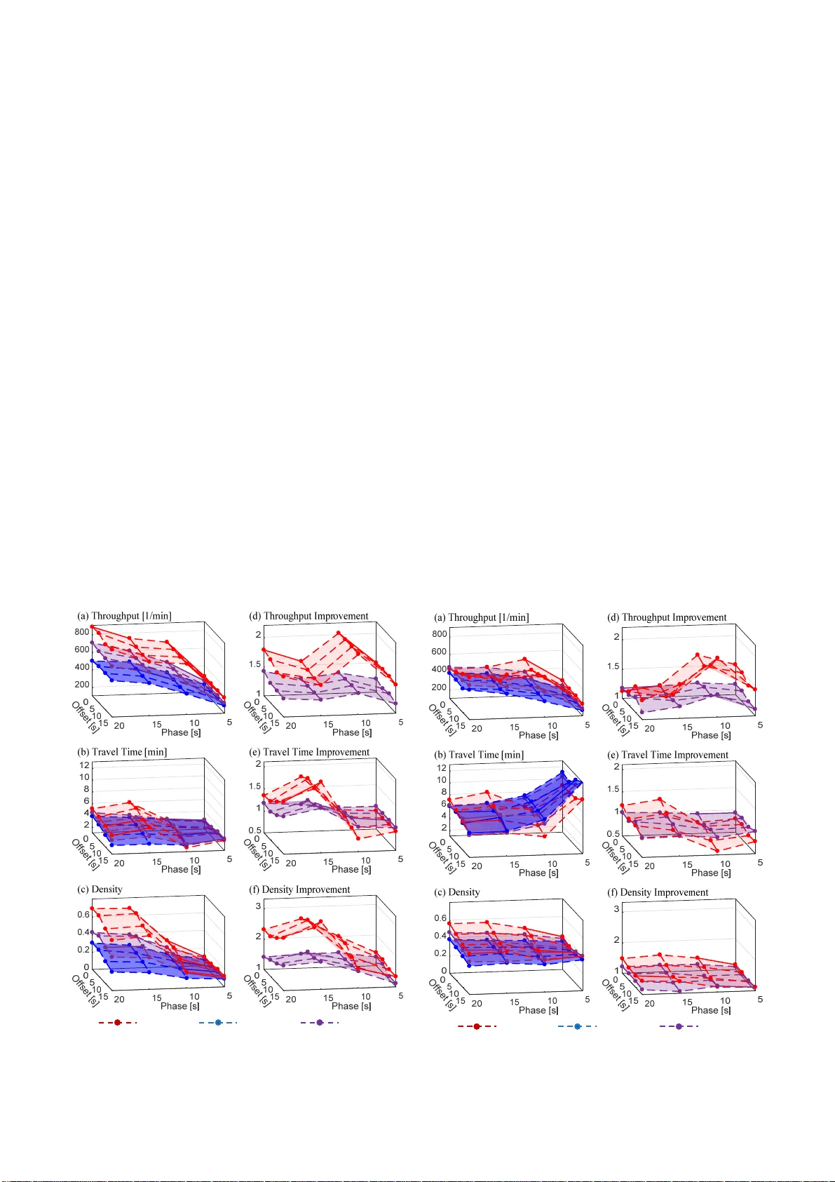
A short ver sion of th is st ud y was pub lished in t he Vehicular Technology S ection in IEE E Access und er the title “A numerical stud y on constant spacing polic ies for s tarting plat oons at oversat urated inters ections ” . https:// ieeexplore.i eee.org/d ocument/97 57221 K. Massow, I. Rad usch and R. Shorten, "A Num erical Stu dy on Constant Spacing Pol icies for St arting Platoo ns at Oversatur ated Intersect ions," in I EEE Access , vol. 10, pp. 43766 - 43786, 2022, doi: 10.1109/ACC ESS.2022. 3167424. First version (v1) submitted to IEEE Access on 21 -Oct- 20 21 , resubmission (v2) on 31 - J an - 2022 , accept ance (v3) on 09 - Mar - 20 22 1 Abst ract — Cooperative Adaptive Cruise Control (CACC) systems are con sidered as key potential enablers to improve driving safe ty and traffic e fficiency . They allow for automated vehicle following using wireless communication in addition to onboard sensors. To achieve string stabilit y in CACC platoons, constant time gap (CTG) spacing policies have p revailed in research; namel y, vehicle interspacing gro ws with the speed. While constant distan ce gap (CDG) spacing policies p rovide superior potential to increase traffic capacity than CTG, a major drawback is a smaller safety margin at h igh velocities and string stability can not be achieved using a one-vehicle look-ah ead communication. The h ypothesis of this work is to apply CDG on ly in few driving situations, when traffic throu ghput is of highest importance and safet y requirements can be met due to comparably low velocities. As the mo st relevant situations where CDG could be applied, we identif y starting platoons at signalized intersections. In this paper, we illustrate this idea. Specifically, we compare CTG with CDG regarding its potent ial to increase the capacity of traff ic lights. Starti ng with the elementar y situation of single traff ic lights we expand our scope to whole traffic networks including several thousand vehicles in s imulation. Using real world data to calibrate and validate vehi cle dynamics simula tion and traffic simulation, the study discusses the most relevant working parameters of CDG, CTG, and the traffic system in which both are applied. Index Terms —CACC, Cooperative Adapti ve Cruise Control, Constant Spacing, Traff ic Light, Signalized Intersection, Vehicle Simulation, Tra ffic Simulation, Capacity, Throu ghput I. I NTRODUCTION ACC is the extension of A daptive Cruise Control (ACC), a driver assistance system which au tomatically adjusts the speed of a road vehicle to m aintain a safe distance from vehicles ahead [1]. Today’s ACC system s use radar sensors to measure this distance. CACC extends ACC by additional communication components to exchange information with preceding vehicles. This inf ormation exchange helps to increase the density of platoons of vehicles with activated ACC and to potentially tackle string instabilities occurring in such platoons. String instability in vehicle pl atoons is caused by radar sensor delays and the dynamics of the vehicles and their power trains. To achieve overall string stability, constant time gap (CTG) spacing policies have prevailed in research, i.e. the target distance between vehicles grows with the speed. However, growing distances entail efficiency loss. This fact is reflected by the recent decision of Daimler to cancel their truck platooning program, which aimed on a 0.68 seconds ti me gap (15 m at 80 Km /h) and did not achieve th e expected efficiency in terms of fuel saving [2]. In this work, a constan t distance gap (CDG) policy for CACC is considered. Although CDG can improve traffic throughput enormously, its applicability in real traffic has been proven to be very limited, as it is not suitable to achieve robust string- stability without significant loss of efficiencies [3]. The hypothesis of this work is to apply CDG only in f ew driving situations when the following circum stances occur:  traffic throughput is of high importance.  platoon sizes are short enough that string instability or communication topology complexity can be handl ed, e.g. employing mini-platoon control strategy [3].  velocities are low enough to cover safety requirements, acceleration is smooth and predictable. While there are several use cases in which such conditions prevail, clearly, traffic-light-controlled intersections are one of the most relevant. In particular, th e traffic flow of two crossing streets share one spot in a time duplex manner. Thus, exhibiting the highest possible traffic density on this spot i s of high importance. Intersections controlled by traffic light s in addition provide clearly regulated right-of-way, i.e. during a green light phase, a platoon can pass this spot as a whole without paying attention to the cross traff ic. Moreover, starting up f rom a stop line when the traffic light changes to green results in a smooth and predictable acceleration maneuver. Thus, we will focus on traffic-light-controlled intersections, with other si tuations presented in future work. In what follows we shall assume urban speeds of up to 50 km/h and stable platoons on intersection either achieved by limited length or capable communication topologies [3]. The research questions discussed in the rest of this paper focus on capacity improvement of CDG over CTG at signalized intersections. Our model for car following dynamics is based on the controller design presented in [31], parameterized using real wo rld data. On Constant Distance Spacing Policies for Cooperative Adaptiv e Cruise Control Kay Massow, Ilja R adusch, and Robert Shorten C Manuscript received May 24, 2014; revised July 10, 2014; accepted July 20,2014. Date of publication September 9, 2014; date of current ve rsion March27, 2015. K. Massow is with the Daimler Center for Automotive IT Innovations at Technical Un iversity Berlin, Berlin, German y (e-mail: kay.massow@dcaiti.com). I. Radusch is with Fraunhofer Ins titute FOKUS Berlin, Berlin, Germany (e-mail: ilja.radusch@f okus.fraunhofer.de). R. Shorten is with the Dyson School of Design Engineering, Imperial College London, SW7 2AZ London, U.K. (e-m ail: r.shorten @ im p erial.ac.u k ) . 2 Comment: Before proceeding some comments on string stability are in order. Altho ugh string stability is an important aspect for realizing CDG in platoons (see related work in the next section), we do not address string stability nor related control theory in this work. Instead we f ocus on assessing the traffic performance of CDG over other spacing policies. Whi le there are many other publications dealing with string stability, the rationale for this work is the usefulness of pl atoons, string stability permitting, in the context of specific use-cases. O ur objective here is to study one such situation in detail, and to illustrate the effectiveness of platoons in an elementary situation in which string stability is not likely to be a serious technical issue. A. Main findings of this work and th e structure this paper Assessing the benefit of CDG for signalized intersections requires a comp rehensive and thorough consideration of a whole traffic system. This includes many microscopic and macroscopic aspects and aggregating partial results. From the authors’ perspective, these should be presented as a whole and not be split apart in different papers. With this in mind our paper is structured as follows. After discussing related work in the Section II, the remainder of the paper is struct ured as follows.  In Section III, we define our research scope and asses the CDG capacity improvement at a single traffic light on a straight road. For this purpose, we parameterize a CDG policy for vehicle simulation using real world data. CDG shows traffic throughput improvement over the CTG baseline of up to 140%.  In Section IV, we extend our study to a whole intersection, in order to cover traffi c related aspects which lo wer the throughput, e.g. turning vehicles and right-of-way. Vehicle simulations, including 160 vehicles, showed that these aspects can lower the CDG throughput imp rovement down to 27% in worst case. We f urther found that CDG benefit on throughput grows superli near with the CDG penetration rate among vehicles.  In Section V, we present a method to calibrate a traff ic simulation model using vehicle dynamics simulation. This is a prerequisite to em ploy many thousands of vehicles to simulate CDG in a whole traffic system, while generating the same results as the vehicle dynamics simulation regarding relevant metrics.  In Section VI we study the impact of CDG on m utually influencing intersections of a traffic system. A synthetic arterial scenario of five intersections revealed that CDG situationally creates backlogs of adjacent intersections, which block the cross traffic. A syntheti c grid scenario of 25 intersections revealed that CDG is vulnerable to create gridlocks. We show the impact of these eff ects on traffic throughput and how to tackle them by adjusting the traffic light configurations regarding green light times and o ffset.  In Section VII, we compl ement our findings with studying CDG in a real world road network simulation scenario including ten intersections in Berlin, Germany. CDG gains a throughput improvement of 70%, while a penetration of 50% CDG reached an improvement of 25%. To exhibit its full potential in urban traffic, CDG needs to enable cu tting in and to prevent junction blocking by cooperative aspects. We conclude this paper in Section VIII. In order to help the reader to follow the f indings arising throughout the study, each section concludes with a discussion of its main findings. II. RELATED WORK The most relevant goals for the d esign of CACC systems are to create small gaps between vehicles to increase road capacity, guarantee string stability [5], while k eeping the communication topology realizable, i.e. as sim ple as possible [1]. The latter is, in the best case, reduced to each v ehicle in a platoon receiving data from its direct preceding v ehicle. Further possible communication structures may include receiving data f rom the platoon leader, multiple predecessors, the successor, or from a fully networked platoon [26]. Each of them entail different advantages regarding control quality, string stab ility and, thus, on the minimum gap size. Further goals on control optimization are ride comfort and fuel/energy consumption, which are both dependent from acceleration profiles. A. Constant Time Headway Policy (CTG) The constant time gap policy refers to maintaining a time gap between vehicles in a platoon, which means that the gap increases with the velocit y. It has received most attention in t he literature for being known to improve string stability even with the simplest communication structure [5], [6]. It also contributes to safety, driving comfort, and imitates the human driver behavior. However, the downside of the v elocity dependent gaps is the platoon length growing with the velocity and the associated required road space. Even very s mall time- gaps of 0.6 s [7] relates to additional road space of 8 m at 50km/h compared to stand still. B. Constant Distance Gap Policy (CDG) The constant distance gap policy refers to a fixed gap between vehicles, independent form the velocity. This policy entails the maximum efficiency in term s of road capacity, however string stability cannot be achieved using the information of the preceding vehi cle only. In [8] it was shown that including additional information from the plat oon leader is required. In order to address string stability, further communication topologies like mini-platoons or multiple vehicles look ahead are reviewed in [3]. Cyclic as well as bidirectional communication is discussed in [9]. C. Adaptive Headway Policies There are different approaches that either combine CDG and CTG in one policy, or further include different control goals by making the gap dependent from more parameters than velocity. In [10] a variable tim e gap (VTG) policy is proposed, takin g traffic flow aspects into account fo r calculating the desired gap. Further work has been done to integrate safety aspects and vehicle limitations in the spacing [11], or to adapt it to human behavior [12]. These adaptive policies gain their positive eff ect mostly at shorter distances at lower speeds com pared to CTG. 3 D. Cooperative Maneuvers Regarding Cross/Parallel Traffic Another important aspect regarding the spacing of CACC platoons, is related to cooperative m aneuvering [13]. Since platoons need to allow for cut-in m aneuvers of other vehicles, the required gaps have to be provided on demand. For urban applications, cooperation is especially required at intersections when platoons need to be crossed by oth er vehicles. Such applications [14] which extend CACC to accommodate cross traffic and parallel traffic are cu rrently researched e.g. in the German research project IMAGinE [37]. Its applications relevant for remainder of this work are cooperative lane merging and cooperative decentralized intersection to ensure clearing intersections for cross traffic. E. Cooperative Start-Up at Intersections In the field of combining CACC with traffic-light con trol, most research aimed at synchronization of platoons and green lights phases, so that stop and go can be prevented, such as [15]. Very few works focus on start-up control coordinated among vehicles and traffic lights, so that as m any vehicles as possible can pass an intersection after stand still. [16 ] studies platoons of vehicles waiting in front of a traffic-light regulated intersection, using SUMO [38]. A coordinated start-up initiated by a V2X message SPAT (SAE 2735) of the traffic light is proposed and the underlying algorithm also addresses the p roblem of low market penetrations. [17] considers a cooperative start-up of real world platoons at traffic lights. Findings indicate that a constant and preferably small gap is essential for increasing the throughput at traffic light regulated intersections. [18] presents an automatic start-up control to start up vehicles with less delay (47.2%) to improve traffic throughput, while [19] addresses an optimized acceleration profile to reduce fuel con sumption. F. Platoons in Signalized Networks In order to assess the im pact of CACC on whole traffic systems, it is not sufficient to consider isol ated traffic lights and intersections. In fact, multiple mutually influencing intersections such as signalized arterials need to be considered. This becomes especially relevant for dense platoons of vehicles passing. [20] presents and algo rithm to optimize signals at arterials based on real-time platoon information. Different penetration rates are evaluated on an eight-intersection arterial using the VISSIM simulator. While most other research in this field focus on the control of traffic lights, [21] addresses optimization from the p erspective of the vehicles in a cooperative way. Clusters of vehicles are formed that approach and depart at intersection on signalized arterials. The approach requires a penetration rate of 100% and aims on increasing traffic throughput while reducing energy consumption. [25] showed, by means of a 16-in tersection arterial, that throughput can be doubled by reducing hum an delay and time gap without changing the signal control. [22] and [23] ai m on preventing stops by slowing down until the queue waiting at the intersection starts moving. Penetration rates lower than 100% are considered in [22]. In [24] splitting up platoons and predicting trajectories aim on ideally passing green l ight phases. However, this requires a certain space while approachin g the intersection and may hardly work f or arterials with sm all intersection interspaces. III. SINGLE TRAFFIC LIGHT PERFORMANCE In this section we begin researching th e performance of CDG on a single traffic light, bef ore considering whole intersections and traffic systems in the subsequent sections. For this purpose, we first need to define a baseline for comparison with other spacing policies and how performance can be m easured. In this regard, we define the research scop e of this work, including preliminary assumptions. From this scope, we derive the determining working parameters for all policies e.g. the standstill distance, as these param eters have a big influence on the performance. Once these parameters are identified, w e use real world data to calibrate them. Finally, we describe the implementation of the p olicies we use for sim ulation with the PHABMACS simulator [15] and we evaluate th e results. A. Research Scope The most relevant m etric to assess traffic light perfo rmance is its capacity, which is defined by its maximum throughput, i.e. the maximum possible number of vehicles passing per time unit [27]. The relevant relationship between throughput and platoons passing the traffic-light, hence, is the number of vehicles per platoon length. The portion of platoon length pertaining to each vehicle in a CTG platoon is depending on the parameters depicted in Fig. 1. The constant portion is the vehicle length plus the standstill distance, while the dynamic portion is the time gap, which grows with the platoon velocity. The dynamic part is zero in CDG platoons, i.e. the CDG platoon len gth is always the same like in standstill, which makes the CD G so effective. Another relevant parameter, especially f or the start-up at traffic lights, is the drivers’ reaction time. This tim e refers to the delayed start-up of a vehicle in the platoon with regard to the start-up of its preceding v ehicle. In contrast to CTG, wh ich is similar to hum an drivers’ vehicle following behavior, C DG can hardly be realized by humans. Thus, for CDG we assume a fully automated longitudinal control w ith no driver in the loop. This consideration is especially relevant for the start-up at traffic lights, as human reaction time would make notable difference here. Since we aim on comparing the f ollowing behavior of CDG with other policies, we neglect the reaction time for all policies in t his work. Accordin gly, in order to compare CDG with CTG, we need to parametrize the constant portion , vehicle length and the stand still distance with the same values. Furthermore, these values should be chosen as realistic as possible for com parison, as their ratio to the tim e gap makes a considerabl e difference. Finally, Fig. 1. A platoon of i vehicles, where l i is the length, r i is the standstill distance, h i is the time gap, ng i is the net gap, and gg i is t he gr oss g ap of the i th vehicle in the platoon 4 we also need to parameterize the time gap of CTG as realistic as possible. Indications for all these param eters could be derived from HCM [27] and the German HBS [28]. The HCM indicates a capacity on average roads of 2400 vehicles per hour, while the HBS indicates 2000 vehicles per hour. Besides the fact that both values differ considerably (gross time between vehicles of 1.8 s and 1.5 s) we have no indication on how to split that time in the dynamic and the constant portion . Recent work [14] on the other hand indicates that time gaps for CTG of below 0.6 s (the dynamic portion only) can be realized for string stable platoons with automated CACC. Remark: Due to th is large range of reasonable values, we decided not to define our baseline for comparison based on theoretic values from the standard works such as [27], nor on best possible time gaps a chieved in current research, such as [14]. Instead we decide to assume for this study, th at future CACC distance behavior in series production will be of similar performance as skilled human drivers and wit h no reaction time. For this purpose, we derive our baseline (time ga p and standstill distance) from real world data collected during the field trial simTD [29 ]. For the sake of fairness, in this section, we will also present results of using parameterization of best achievable time gaps of current research. We further assume that the velocities in our study is low enough so that CDG can keep the standstill distance. The resulting parametrization is presented in the nex t subsection. Furthermore, as earlier m entioned, CDG should not be applied at arbitrary high v elocities due to safety aspects an d stability issues arising when the one-vehicle look-ahead communication pattern is ap plied. Thus, there is a spee d limit at which the CDG spaci ng policy is required to be switched to CTG. As most traffic light scenarios are locat ed in urban areas we limit our study to veloci ties below 50 Km/h. For the sake of completeness, we define and st udy a policy that switches from CDG to CTG at 30 Km/h. This policy will be referred to as SWITCH in the remainder of t his work. B. Calibration of Simulation on Real World Data As motivated in the previous subsection, we employ real world data to calibrate th e policy parameters for simulation, as well as the baseline for evaluation. The data we used has been captured at simTD [29], a larg e scale field trial for testin g V2X applications conducted over a period of six month, including a test fleet of 100 controlled vehicles. For the calibration of t he simulation model, we consider start -up situations at traffic lights. The relevant calibration data for parameterization includes the acceleration profile in order to model the first vehicle of a platoon, the standstill distance and the time gap. Therefore, we filtered situations from the logged test data according to the following constraints:  start-up after standstill, preceding vehicl e is present;  vehicle accelerates, target speed 40km/h – 65 km /h;  accelerator is not released during the situation. The filtered data included 3,546 start-up situ ations from 27,642 logged trips d riven by 98 different drivers (73 male, 25 female). Fig. 2. depicts the resulting data, inspired by the m odel matching process for acceleration maneuvers described in [13]. All situations were aligned time-wise, at the point time when the preceding vehicle starts moving. The resulting curves of velocity and distance to the preceding vehicle were averaged. The averaged time gap settles at 0.87 s and the average standstill distance is 2.95m. We used t hese values to f eed our simulation models. The black dotted lines represent the 95% confid ence interval, which m ark the band for simu lation model validity according to [13]. We calibrated the a cceleration profile of the platoon leader in our simulation to match the average speed trajectory of real world data. The speed profile in simulation matches the confidence band of t he real world data, except for some dents in the graph during gear shifts. Thus, we consider the simulation model as valid representation of the real world data. In this way we w ere able to determine all relevan t parameters as defined for our research scope, except f or the vehicle length. For the vehicle length we assum e 5.15 m due to the following considerations. According to [30] in 2011 we can assume an average length of passenger vehicles of 4.75 m. We add further 0.4 m to represent the increased length of vehicles since 2011 and some heavy duty traffi c. C. Spacing Policies Using the parameters derived in the previous subsection, we finally define the following spacing policies for studies in simul ation. 1) CDG-Constant Distance Gap The constant distance gap policy CDG is defined by the vehicle length of 5.15 m and the stand sti ll distance of 2.95 m determined in the previous subsection. 2) CTG-Constant Time Headway According to the calibration with real world data we de fine the baseline policy for this w ork with 0.87 s time gap, in the following referred to as CTG-Ref . At 50 Km/h a gap of 15 m is reached. For comparison, we also def ine a policy CTG- HCM to match the American HCM a t maximum speed in urban areas (50 Km/h). Assuming the gross ti me gap between vehicles of 1.5 s (HCM at 2400 vehicles per hour) together with vehicle length and standstill distance (as defi ned above), this results in a net time gap of 0.9 2 s. CTG-HBS represents the German HBS 5 1 0 1 52 02 5 3 03 5 Time [ s] 10 20 30 40 50 60 Distance driver avg.  [m] Speed  driver av g.  [km/h] Averaged distance [m] Average  speed [km/h] Conf.  intervals Time  gap [s] Speed  simulation [km/h] Speed  pred ecessor [ km/h] Fig. 2. Averaged Velocity and following distance proc essed from real w orl d start-up situations to derive CDG and CTH controller parameters 5 with 2 000 veh icl es per hour and, th us, with 1.22 s ti me gap. 3) Switch Based on the parameters of CDG and CTG-Ref we define two polices to switch between both of them at a predefined velocity of 30 Km/h. SWI TCH- 1 renders the time gap using the difference between the current velocity and 30 Km /h, i.e. at 50 Km/h a gap of 6 m is reached. SWITCH-2 increases the gap from 0 m at 30 Km/h to 15 m at 50 Km/h, so that the same distance as with CTG-Ref is reached. 4) Mix In order to enable studying a certain rate of CDG penetration, we define the Mix p olicy. The penetration rate is set to 50 % with a randomly alternating pattern on CD G and CTG-Ref . D. Realization All spacing policies described above haven been implemented in the PHABMACS simulator [13], for subsequent evaluation. Further, all policies rely on t he one- vehicle look-ahead communication pattern [26]. The evaluati on scenario simply consists of a straight single lane road with a single traffic light, generated manually. In order to m easure the maximum achievable throughput of all policies we create the same initial condition for each policy simulated. All vehicles approach the traffic light while red and queue up to standstill at the stop line. Once all vehicles have stopped the traffic lig ht turns green and the platoon starts accelerating up to 50 Km /h. Vehicles passing the stop line are counted for evaluati on. 1) CTG The basis controller for the vehicles is a Java implementation of the cascaded PID framework presented in [31] (see Fig. 3), integrated as longitudinal controller in th e PHABMACS driving controller hierarchy (see [13] f or explanation). As the controller design is discussed in detail in [31], we just brie fly describe its main components.   represents the low-level controller  acting on the veh icle model  , where  r epresents the   vehicle in the platoon.  is different from the low-level controller in [5] and was initially presented in [32]. The input of  is the control value   represented by the desired acceleration of the vehicle, while the output is the desired torque for the engine and the brake, which are fed directly to the vehicle model as described in [13].  ,  is a PD-type feedback controller that acts on a locally sensed distance to the preceding vehicle with a simulated sensor delay of 150 ms.   implements the spacing policy. Fo r CTG the policy   is defined by 1 +  ,  [31] (here s is the Laplace transform variable) which is the transf er function representation of  ,     ,   in the time domain, where  , is the desired spacing,   is the standstill distance,  , is the time gap and   the velocity.  , is a feedforward filter described in [31] using the communicated information of the directly preceding vehicle, i.e. the current and de sired acceleration   and   , as well as t he current time l ag of the vehi cle model    . In contrast to [31] we treat   as a dynamic value for each vehicle, which is taken online from a calibrated m ap depending on the current gear, requested torque (drive/brake), and current engine rotational speed. 2) CDG For the CDG poli cy, two aspects differ from the setup described above. The spacing policy   is expressed by  ,    in the time domain and   1 in the frequency domain. The feedforward controller   , is the implementation of the optimization problem depicted in Fig. 4. An acceleration curve is predicted for the preceding vehicle, based on the received information   󰇛󰇜 ,    󰇛󰇜 , and   󰇛󰇜 . Taking the latest measured communication delay into account,   is calculated so that   meets   in a predefined time interval in the future. 3) SWITCH By combining CDG and CTG according to the parameters described above, we realized SWI TCH as a simple change between both policies at 30 Km/h. E. Evaluation Fig. 5 depicts the results of six sim ulation runs with one graph each for the seven des cribed polices. The graphs ca n be interpreted as a vehicle counter passing the traffic light stop line over time. The counter starts at time 0 when the traffic light turns green after red. The vertical lines in the f igure mark the throughput of different green phase len gths. The throughput of the alternative spacing policies for a specific green phase leng th can be read from the figure at the point where its vehicle counter graph crosses the vertical lines. For inst ance, the number of passing vehicles at a green phase of 15 s is 17 for CDG , 13 fo r SWITCH1/2 , 11 for MIX , 8 for CTG-Ref , and 7 for CTG- HBS . In order to enable comparing the performances of all policies at each phase, we exceptionally applied a deterministi c alternating pattern on the Mix policy. In this way we create the same portion of CDG for each phase. The shift between the time scale Fig. 3. Control structure of the longitudinal model Fig. 4. Concep t of the p redictive CDG feed forward co ntroller, wh ere   is the current point in time,   is the next future point in time,   is the communication delay, n is th e length of the acc eleration trajectory [    ..   ] 6 in Fig. 5 and the vertical l ines representing the green phases is caused by the yellow phase of three seconds. Note that at time 15[s] the platoon leader reaches m aximum speed of 50 Km/h. In case of the CDG policy that means the whole p latoon is already at maximum speed and CDG can fully exhibit its performance benefit. Accordingly, its throughput graph turns from a curve into a straight line. In case of CTG , in c ontrast, vehicles start moving one by one, while the CDG platoon is moving as a whole from the point in time when the platoon leader starts up. This is the key eff ect which makes CDG effective at traffic lights. For a more performance oriented view on the results, Fig. 6 compares the throughput improvement of all policies with the baseline CTG-Ref over ti me. While the throughput improvement of SWITCH1ch and MIX reach their saturation around 50 % around 20 s, CDG approaches an improvement of about 140 %. In order to illustrate the impact of different standstill distances, we ran one simulation with the double standstill distance of 6 m (CDG-6m) . It improved the throughput by 70%. F. Conclusion Our studies of CDG on start-up at a sin gle traffic light show a performance benefit over CTG and the other policies. This performance benefit grows with the green phase length, and reaches 120 % at 10 s green time and then reaches a saturation of around 140 % for longer green phases. A penetration rate of 50 % CDG in a mix with the baseline policy only reaches 45 %, i.e. the CDG benefit does not scale linear with the penetration rate. In order to provide a com parison between the policies, the base parameters of the policies were calibrated on real world data and human reaction time was neglected. It m ust be noted, that for green phases of more than 30 s, th e CDG plat oon exceeds a length of 43 vehicles, which already coul d give rise to string stability issues. For that reason, for a real world implementation, counter measurements such as splitting up into mini -plat oons mu st be con sider ed [3], w hich m ight aff ect th e performance. The SWITC H1 policy, which switches from CDG to CTG at 30 Km/h reaches a performance gain of 60 %. IV. SINGLE INTE RSECT ION PERFORMANCE In this section we expand t he analysis of CDG from a sing le traffic light to a whole intersec tion. The performance of CDG policies, described in the previou s section, are to a large ext ent due to the fact that th e platoon could pass the traffic light in a free flow. However, at whole intersections the impact of traffic flow reducing factors need to be taken into account for performance comparison. This in cludes reduced velocities while turning, stops due to g iving way while turning, as well as the fact that green light phases cannot b e arbitrary long as they share the full cycle time with cross traffic and turn phases. As before, we start with the definition of an intersection layout that covers all aspects relevant for this research. Subsequently, we define further metrics to assess CDG perfo rmance at intersections and we finally evaluate results gained from simulating a whole intersection. A. Intersection Layout and Simulation Setup Intersection layouts in urban areas include many possible constellations of elements which may have eac h different impact on the performance of CDG [27], [33]. As we have to handle and permute many paramete rs apart from the layout, our objective now is to define a reference layout that covers as many layout related aspects as possible and can be a fixed parameter for further studies. Note t hat a literature review ended up with no results on the question of what are realistic portions of left and right turning vehicles. We, thus, decide to permute both as parameters of the simulation. Fig. 7 depicts our reference layout with two lanes in each direction. Each right lane mixes straight driving with protected right tu rning vehicles, as there are no pedestrians. Each left l ane mixes straight driving with unprotected left turning vehicles, which always need to wait for oncoming vehicles. This is ensured as there are always more vehicles waiting in front of red traffic lights from each direction than can pass it during the green phase. This oversaturation at the intersection inlets i s also necessary to allow the different policies to exploit its full potential of passing vehicle per green lig ht phase. The radius of the intersection is 20 m and turning velocity is 7 m/s which results from a maximum lateral acceleration of 2.5 m /s² [34]. Left turning vehicles entering the i ntersection consequently block their lane until the end of the green light phase. This reduces the random effect s in the resulting throughput, independent from the desired parameterization of the simulation. We choose this particular intersection l ayout due to the following considerations. We should cover protected Fig. 5. Throughput comparison for the diff erent spacing policies 0 5 10 15 20 25 30 Time  [s] 0 5 10 15 20 25 30 35 40 45 Phas e:5  s  Phase:10  s  Phase:15  s  Phase:20  s  Phase:25  s  CDG CTG ‐ Ref. CTG ‐ HBS CDG  Mix  50% Switch1 Switch2 Vehicle Count [ 1] CDG ‐ 6m Fig. 6. Throughput improvement compar ison for the different spacing policies 50 100 150 200 250 5 1 01 52 02 53 0 Throughput [%] Time  [s] 7 turning (turning signal phase - no yielding required) due to the reduced velocity while turning and unprotected turning (yielding required) due to it s blocking effect on the f ollowing vehicles. We do not need to consider dedicated turning lanes, as they would just shift the block ing effect to occur at a higher portion of turning vehicles. We also do not need to consider dedicated traffic light phases for turni ng, as we already cover protected turning. We also deci de to avoid lane changes in the whole scenario, in order to ex clude the impact of lane changes on the simulation results. Lane changing is difficult to model, it depends on many parameters of rand om character, and we have no ground truth for calibration. Lane changing would further enlarge the parameter space for our sim ulation, while having a considerable random influence on the results. For the metrics discussed in the next subsection, m issing lane changes are only relevant for the travel time of single vehicles on the blocked left lane when the right lane is free. However, we assume these to be averaged out by faster vehicles on the rig ht lane. B. Metrics For comparing the performance of CDG and CTG at intersections, we basi cally measure the m aximum intersection capacity [28] for both. While oversaturating th e intersection inlets, we choose to measure the following m etrics:  throughput – vehicles passing per tim e;  travel time – average time vehicles nee d to pass;  densit y – po rti on of roa d met ers occu pied b y vehi cles . Note that the German HBS and the American HCM [27], [28] define the metrics for sign alized intersections based on waiting time and waiting queue length in front of traffic lights. They also consider the adjustment factors which are to be taken into account while designing signalized intersections. These metrics are not suitable for our study, as we are not aiming on optimization of configuration for the traffic light. Furthermore, measurement of waiting times contradicts our approach of oversaturating the inflows of the intersection, which is required to reveal the full potential of CDG. Thus, we decide to apply the metrics defined by HBS for open roadways (throughput, average speed, densit y) and permute the configuration parameters of t he traffic light setup. Instead of average speed, we measure the travel ti me, as it is independent from the actual travelled distance, which is difficult to be determined for random routes in SUMO [35]. The configuration parameters to be permuted are the green p hase length and the ratio of left and right turns per lane. C. Evaluation As earlier stated, o ur goal is not to f ind an optimization for the traffic light setup but to study the per formance of CDG vs. CTG under all potentially occurring traffic conditions. In order to map this span of conditions, the sim ulation ran with 504 permutations of the following conditions, as motivat ed in the previous subsections:  Intersection layout is fixed.  Traffic flow at the intersection inlets is oversaturated, so that there are always m ore vehicles waiting at a red light than can pass during one green phase.  Port ion of righ t (0%, 10%, 3 0%) an d lef t t urns (0 %, 5 %, 15 %, 30 %) are permuted.  Penetration rate of CDG and CTG are permuted with (0 %, 10 %, 25 %, 37 %, 50 %, 75 %, 100 %).  Green light phase is permuted from 5 s to 30 s. In one permutation, the green time is th e same for all directions.  Simulation time is five full traffi c light cycles. The intersection layout and the simulation setup as described in Section IV.A, as well as the policies as described in Section III.C were implement ed in the PHABMACS vehicl e simulator [13]. Fig. 8 depicts a view on the intersection during simulation. The colored circles represent the radius for travel time measurement (40 m) and density (20 m ). Throughput is calculated from vehicles leaving the 20 m radius per time. For the randomness to generate and equally distribute turnings and penetration ratios, PHABMACS employs the Mersenne Twister algorithm [36]. On average around 160 vehicles were in the simulation at the same tim e, 40 vehicles per direction. The results of the simu lations for 15 s green phase, captured in accordance with the previous section, are depicted in Fig. 9. The throughput of different CD G penetration rates is depicted in vehicles per hour on the vertical axis, f or each permutation of left and right turn ratio on the horizontal axis. The highest throughputs were measured with no turning vehicles, at 11,550 CDG and 5,254 CTG-Ref , an improvement of 120%. The lowest throughput at 30% right turns and 3 0% left turns is at 4,281 CDG and 3,016 CTG-Ref , an improv emen t of 42 %. The improvement without turning is similar to the Fig. 7. Four way, two lane refere nce intersection layout for simulation Fig. 8. Simulation of a single in tersection in PHABMACS simulator 8 improvement measured at a single traffic light in the previous section. With a ratio of 30% right turns on the right lane, the improvement falls to 88% due to the reduced velocit y while turning. Additional 30% left turns on the left lane alm ost stops the throughput on the left lane, i.e. all vehicle passing the inters ecti on ar e affec ted by the reduc ed spe ed of the righ t turn s, which results in a drop of t he improvement to 42%. The travel time drops from 55 s ( CTG-Ref ) to 34 s ( CDG ), which corresponds to a travel tim e reduction of 38 %. The lowest time reduction of 12 % results with 30 % l eft turns and 30 % right turns. Throughput and travel time reduction correlate with an increased density on t he intersection. While the average densit y of CTG-Ref is a roun d 35 % for all per mutati ons, the density of CDG depends visibly on the turning ratios. With no turns, the density f or CDG peaks at 47 %. For different CDG penetration rates, the same superlinear impact becomes apparent on throughput, travel time and density. At the first glance all graphs seem to follow an approximately uniform course. However, there are some irregularities recognizable in the pattern due to the random ness in the simulation, which affects the measured result at certain co nstellations during the simulation. For instance, at 5 % left turns, 10 % right turns and 50 % penetration, the throughput is the same as with 25 % penetration due to that circumstance. Moreover, although the travel time falls with an in creasing CDG penetration, the travel time gain is of less m agnitude as the throughput improvement. This is due to the fact that during the red for all directions portion of the traffic light cycle, no time benefit can be achieved by CDG . Discretization effects of the traffic light queue, become apparent at 15 % lef t turns and 25 % penetration with a higher throughput than for CTG-Ref, yet wit h a higher travel time. Table 1 finally summ arizes the throughput improvement over CTG-ref at all green light phases simulated. All values are rounded to the depicted number of digits. For the sake of simplicity, the table only lists the extreme values of 100 % ( CDG ) and 50 % ( Mix ) penetration with no turns, 30 % right turns only, 30 % left turns on ly, both at the same time. The penetration dependent improvement ratio (PIR) on the throughput is calculated by   to compare the im provement of CDG and Mix . While th e absolute improvement of CDG falls with falling green phase and increasing turning ratio, the PIR grows for short green phases and high turn ratio. At 15 s green phase length with lef t and right turns, the PIR p eaks at 0.55 for 50 % penetration. D. Conclusion In thi s sec tio n we broa dene d th e stud y of CDG from a single traffic light to a whole intersect ion, including different ratios of protected and unprotected turning. As expected, the presence of turnings at the intersection reduced the benefit of CDG compared with a single traffic light. The lowest benefit was measured at 10 s green phase lengt h, where the throughput impro veme nt s hrank fro m 81 % withou t tur ning to 2 7 % wi th turnings. The specific impact of turnings depends on presence and length of turning lanes. In our studies we omit such lanes in order to reduce parameter space. Thus, in our studies, one turning vehicle already blocks a complete lane. 0 2 4 6 8 10 12 100% 75% 50% 37% 25% 10% 0% CDG Penetr ation Vehi c les P as sed per H our [1000 ] Left 30 Right 40 50 60 70 Travel Time[ s] 00 . 1 0 . 3 00 . 1 0 . 3 0 0.1 0.3 0 0.1 0.3 0 0.05 0.15 0.3 Turning Ratio 30 40 50 Density [%] Fig. 9. Throughput, travel time, density on a single intersec tion CDG vs. CTH TABLE 1 T HROUGHPUT IMPROVEMENT OF CDG AT SINGLE INTERSECTIO N Turn ratios Metric Green Phase [s] 5 10 15 25 25 30 no tur ns CDG [%] 50 81 120 134 140 135 Mix [%] 21 25 33 41 42 37 PIR 0. 42 0.31 0.27 0.30 0.30 0.27 right turns 30 % CDG [%] 50 64 85 91 94 107 Mix [%] 21 19 25 28 29 28 PIR 0. 42 0.31 0.30 0.31 0.31 0.26 left turns 30 % CDG [%] 45 64 94 92 112 109 Mix [%] 19 26 17 21 29 30 PIR 0. 43 0.42 0.18 0.23 0.26 0.28 left + rig ht turns 30 % CDG [%] 59 27 42 50 45 46 Mix [%] 28 10 23 21 16 19 PIR 0. 47 0.39 0.55 0.42 0.35 0.41 9 Summary of Section IV : Vehicle simulations, including 160 vehicles, showed that th e presence of turnings at the intersection can lower the CDG throughput improvement to 27% in worst case, co mpared with 140% at a single intersection. The CDG penetration rate among CTG has a nonlinear effect on its benefit. This fact is a potential hurdle for market-introduction. However, with falli ng absolute benefit of CDG, due to high turning rates and short green phases, the relative benefit of CDG penetration rate increases. V. MODEL CALIBRATION FOR MACROSCOPIC SIMULATION The next step for our studies on CDG i s to evaluate its impact on whole traffic system s, i.e. on multiple mutually influencing intersections. As motivated earlier, developm ent and evaluation of longitudinal control like CACC in sim ulation requires realistic mapping of physics. Fine differences in m apping physics and the control system interacting with its environment may lead to considerable differences to t he resulting behavior. Thus, for studying CDG at a sin gle traffic light, the sub- microscopic vehicle simulator PHABMACS is the appropriate tool (for explanations of the terms microscopic, macroscopic, and sub-microscopic simulation models see [13] or [39]). Thanks to its ability to scale out physics and control algorithms, simulating a whole intersection i ncluding hundreds of vehicles for hundreds of simulation runs is enabled [13]. However, in order to re search whole traffic systems including many thousands of vehicles, PHABMACS becomes out of scope for two reasons. First, mapp ing that many vehicles would still require considerable time and computation capacity. Second, traffic systems under research from such macroscopic perspective may also produce realistic results, provided that an appropriate model is leveraged, which maps the microscopic behavior sufficiently in a macroscopic scale. In the following, we propose a m ethodology to calibrate and validate a sub-microscopic simulation model against a microscopic simulation model, in order to enable macroscopic traffic analysis including several thousand vehicles. We use this methodology to match the implementation of CACC controllers in PHABMACS and its validated vehicle model to the SUMO [38] traffic simulator. Calibration and validation are essential here in order to ensure that the traff ic simulation model in SUMO generates the same results regarding relevant metrics as vehicle dynamics simulation model in PHABMACS. A. Mode l In order to map CACC in SUMO, we ch oose the Krauß car- following model [39] as the basis implementation. The model is directly applicable for CTG. For CDG, however, w e need an adaption of the model, as fixed following distances cannot be realized for t he following reason. Alth ough, the Krauß m odel has a parameter for the velo city dependent time gap, setting this parameter to 0 s does not make the vehicles start up at the same time. Each vehicle starts exactl y one simulation time step later than its predecessor. Since all vehicles follow the same acceleration trajectory, the i nter vehicle distance is constantl y growing while accelerating and shrinking while decel erating. For this reason we modified the Krauß m odel according to (1). As with the Krauß m odel, we base our m odel on the calculation of a m aximum safe speed   . If th e dista nce  to the predecessor is greater than the stan dstill distance   , we apply the Krauß model with a small modification. The tolerance band    is added to   for the calculation. In this way, a tolerance band around   is created. This allows the vehicle to overshoot the stand still distance by   , which is requ ired as a buff er for driving with constant d istances. If the distance  is within this tolerance band,   is set to the pred ecessors velocity   . If the band is undershot,   is set to the   reduced by a factor  (0.95), to make the vehicle return to the tolerance band. The simulations step size needs to be aligned with   , in our case   equals 0.5 m at a simulation step size of 0.1 s.                              2󰇛   󰇛     󰇜󰇜   (1) This looks like a hack of the car-following-system designed for SUMO and we would recomm end to use this model for specific applications only. However, f or our use-case, it works sufficiently good, as demonstrated in the next subsection. Another required modification, is to enable followers to catch up with their predecessors who drive with maximum speed. For this purpose, we lowered the maximum speed of vehicles without predecessors to 95% of the speed restriction of the current link in SUMO. This is also do ne for the Krauß model. B. Calibration and Validation Method Our proposed validation methodology consist of two steps. First the models of bot h simulations, vehicle simulation (PHABMACS) and traffi c simulation (SUMO) are calibrat ed. This calibration aims to the match of ti me and location of each vehicle during the simulation for the same scenario in both simulators. Second, the m etrics determined to evaluate simulation results, are determined in both sim ulators for the same scenario and validated against each other. This model validation method was designed following the consideration of balance between effort and valu e of model confidence, presented in [13]. Accordingly, this method does not aim at finding the limits of model validity, but to assure validity of the considered simulation scenario to generate valid m etrics. Fig. 10. Calibration setup SUMO - PHABMACS …… …… … … 100 m 12.5 m 100 m 96.5 m 10 1) Step I Timing In order to calibrate the timing and location of a vehicle (time-space domain), we first need to place detectors in both simulations at crucial, scenario specific locations. In our case our objective is to consider multiple mutually influencin g intersections, i.e. our scenario includes one central intersection and one adjacent intersection in each direction as depicted in Fig. 10. As the intersection layout is iden tical from each direction, we just need to regard vehicles incoming from one direction at the central intersection. The distances between the intersection, as well as the traffic light cycle times and their offset between the intersectio ns are chosen in accordance with the next section. The detectors are placed according to Fig. 10. In this way, start-up characteristics, travel t ime through and between intersections are covered. Again, lane changing is disregarded for the aforementioned reasons. Left turns stop the traffic on the left lane and the turning ve hicle is the only one passing the traffic light for the current cycle . In order to validate that timing in both simulations is similar, we run both simulations for all relevant perm utations of simulation parameters and compare the vehicle counter for all detectors. This is performed automatically, so that the shortest cycle time possible of manually tuning the model parameters and validation is achieved. We need to assure that for all permutations of CDG penetration, traffic light cycle times and offsets, the correct num ber of vehicles pass per traffic light cycle. As the shortest traffic light cycle tim e to be studied is 5 seconds, a lim it for the maximum difference between corresponding detectors in both simulations of 1 second is sufficient. For the assessment of validity, we propose the objective timing criterion as described above, complemented by a subjective criterion as motivated in [13]. If a simulation scenario ran invalid and the num ber of detector that show higher differences than 1 second is s mall, the verdict of validi ty can be changed manually if reasonable. One example for such a subjective verdict is depicted in Fig. 11. While the objective criterion can be applied automatically, th e subjective criterions needs to be assessed m anually. The idea here is to apply automatization to the greatest extent, while reducing manually effort to assess the edge cases. For further inf ormation on this methodology, please refer to [13]. The count on each detectors is depicted with the corresponding color of Fig. 11. The sim ulation ran at a traffic light cycle of 15 s, no offset between intersections, with vehicle queue from south of: 6 left ( CTG ), 6 right ( CTG ), 18 straight ( CTG ), 8 left ( CDG ), 8 right ( CDG ) , 2 1 s t r a i g h t ( CDG ). Around simulation time 150 s, a slight high er compactness of the CTG platoon in SUMO causes a time difference at the intermediate straight detector of 1.2 s. Around time 239 s, the CDG plat oon of 20 vehicl es st ops in fron t of th e north inters ecti on. Th e 15th vehicle stops right on the same detectors in PHABMACS, while in SUMO the corresponding vehicle stops slightly in front of the detector. Thus, a tim e difference of a full cycle tim e is measured. The final parameterization (notation acco rding to [42]) of the SUMO model after calibration is listed below. Fig. 11. Subjective validation criterion – example: gre en light 15 s, offset 0 s 100 150 200 250 300 Time [s] 0 10 20 30 40 50 60 70 Vehicl e count [1] SUM O Phabm acs 1.4 s 21.7 s subject ive judgement required Fig. 12. CDG model metrics validation SUMO - PHABMACS 0 2 4 6 8 10 12 100% 50% 0% Confidence Inter vals CDG Pen etr ati on Left 30 Right 40 50 60 70 Travel Ti me[ s] 00 . 1 0 . 3 00 . 1 0 . 3 0 0.1 0.3 0 0. 1 0.3 0 0.05 0.15 0.3 Turnin g Ratio 30 40 50 Dens ity [%] Vehicles Passed per Hour [1000] 11 2) Step II Metrics Validation In step II, the calibration completed in step I is validated. The approach of our proposed validation method is based on the statistical analysis of the same simulation scenario in both simulators. By proceeding in a similar fashion to the validation of a sub-microscopic simulation model against a real world vehicle in [13], we validate a microscopic traffic sim ulator (SUMO) against a sub-microscopic vehicle simulator (PHABMACS). As described in [40] we employ the 9 5 % confidence interval of the relevant met ric measured at multiple simulation repetitions for analysis. The m etrics to be validated in this case are throughput, density, and travel time. The confidence intervals for each metric depicted in Fig. 12. CDG model metrics validation SUMO - PHABMACS fo r the 15 s phase time simulation run corresponding with Fig . 9. The confidence intervals are determ ined as described in [13], using the MATLAB® implementations of the Student’s t inv erse cumulative distribution function “ tinv ”, and the standard deviation “ std ” for σ , where v is the degree of freedom (the number of simulations, six in this case) and µ is the mean value of dat a. ,    󰇥 ∓   √  󰇦 ,    󰇛 0.95,  󰇜 ,    1  (2) All 504 permutations (see previous section) were simula ted six times in PHABMACS and in SUMO. We consider val idity as achieved if the average metric measured in SUMO is inside the confidence band measured in PHABMACS, which is the case as shown in Fig. 12. VI. MULT I INTE RSECT ION PERFORMANCE In this section, we anal yze the crucial traffic hi ndrance situations caused by CDG, which lead to a decreased performance of CDG comp ared with the single intersection analyzed earlier. Two main f actors lead to such a lowered performance. First, congested intersection outlets that lead to obstructed off-flowing traffic, and second, reduced in-flowing traffic. Both can be caused by the influ ences of the overall traffic system. Thus, the m ain question to be discussed in this context is the impact of CDG on the traffic system , or more precisely on multiple mutually influencing intersections. To proceed, for consistency with our previo us discussion, we apply the same intersection layout. We combine this layout to two synthetic simulation scenarios, an arterial sign alized corridor [41] with five intersections and a coordinated grid network [41] of 25 intersections. Including up t o 5500 vehicles per run, bo th scenarios are simulated with multiple permutations of traffic light configurations and turning ratios. With regard to simulation runtime we can afford such a number of vehicles and this span of permutations, thanks to t he calibration of the CDG and CTG model with the traffic simulator SUMO. The results are calculated counting vehicles entering/leaving the simulation 20 m far from the outer intersections, i.e. exclu ding the unbound queues. All trips end outside this area. Final values are captured when all metrics increased to a steady state level and keep it for five hours simulation time. For all sim ulation scenarios, we assume a maximum possible traffic inflow and an unobstructed outflow of the traffic system. Finally, we model a real world road network simulation scenario using a real world traffic layout and traffic light configurations in the subsequent section. The topology of the arterial scenario and the grid scenario is based on an urban area in t he South of Market neighborhood in San Francisco (see Fig. 1 3). We choose this area as it h as an even grid of intersection a ll with the same distan ce of 276.5m NW bound and 192.5m SE bound. These constant intersection interspaces enable isolating the impact of interspace length on the simulation results from the other simulation parameters. Although this area partially consists of one-way streets in real world, we unify the simulation scenario with two way streets and intersection layouts according to Section IV.A. A. Traffic Hindrance Situations Applying CDG at the constellation of intersection in the described way, leads to three traffic hindrance situations. The disturbance effects resulting from these three situations depicted in Fig. 14 are described in the f ollowing. 1) Situation 1 – Junction Blo cking Assuming the traffic backlog from a traffic light reaches the adjacent intersection as shown in Fig. 14 (a). Under certain circumstances vehicles come to a stop o n the middle of the intersection and do not leave before the traffic light switches to TABLE 2 SUMO M ODEL P ARAMETERS Mode l Parameter in SUMO decel (  ) accel (  ) tau (  ) minGap (   ) Sigma CTH 4 .7 0 1.70 0.9 2.95 0.4 CDG 4.70 1.40 0.02 2.45 (+   0.5) 0.02 Fig. 13. Simulation scenarios arterial and grid base d on urban are in, San Francisco (South of Market) , CA, between Market St. and Harris on St. Fig. 14. Traffic hindrance s ituations (c) Gridlo ck (a) Junction blocking (b) Turn blocking Red / green light Straight- driving Right- turning Kartendaten  ©  2019  Googl e  Deutschland 12 the phase for the cross traff ic. In this situation, the cross tra ffic has to wait for a full traffic light cycle u ntil the intersection is clear again. Due to the close distances in a CDG platoon and the one-vehicle look-ahead pattern, this event occurs m ore often than with CTG. CTG by its very natu re creates a contraction of the platoon while stopping and thereby more space on the intersection area. In order to create spaces o n the intersection, CDG would require a coordination between vehicles, such as described in [37]. In SUMO t here is a heuristic mechanism ( no- block-heuristic ) that helps vehicles to anticipate a possible hold at a position which blocks the cross traffic. H owever, as in the real world, in some specific situations, this predictive mechanism does not alw ays work out. 2) Situation 2 – Turn Blocking Even if vehicles stop to prevent a junction blocking, traffic backlogs might prevent vehicles from turning. In this case, as depicted in Fig. 14 (b), the cross traffic behind the turning vehicle is blocked for the current traffic lig ht cycle. This applies for right and left turning vehicles. This event is also more likely to happen with CDG than with CTG for the aforemention ed reasons. 3) Situation 3 – Gridlock If situation 2 occurs at four intersections at the same tim e, this leads to a com plete standstill beyond subsequent traffic light cycles (see Fig. 14 (c)). For such situations, SU MO offers a mechanism ( teleport [42]) to model the real-life behavior of eventually finding a way around the blocking vehicle and so resolving the gridlock. For all experiments described in the following subsections, we set the waiting time in SUMO for each vehicle to resolve g ridlocks and turn blockings to three full traffic light cycles. Solving junction b lockings is set to the ti me of two green light p hases. B. Arterial Signalized Corridor – Simulation Scenario The arterial scenario consists of five adjacent intersections of a major street with a distance of 192.5 m, as depicted in Fig. 15. The two lane layout of sections IV.A, as depicted in Fig. 7, is applied. The arrows in the Fi g. 15 mark the high traff ic inflows. As described earlier, lane changes are suppressed in order to exclude the imp act of a lane chang e model on the sim ulation results. This scenario represents coordinated intersectio ns on a major street. Thus, the green light portion of the cy cle time is longer for the major street than for the minor s treets. The following parameters were applied for the sim ulation:  turning rates on minor roads: left 2 0 %, right 40 %;  turning rates on m ain road is permuted with two different parameterizations: 1 (no turning), 2 (left 10 %, right 20%);  penetration rates are permuted with 0 % ( CTG ), 50 % ( Mix ), and 100 %( CDG );  green light portion for the m ajor street is permuted with 25 s, 30 s, and 35 s with corresponding 10 s, 7 s, and 5 s for the minor streets;  offset time (time shift between the traffic light cycles) between intersections is permuted with 0 s and 15 s. 1) Impact of Green Phase and Offset Time Between Coordinated Intersections for CDG on Arterials For a better understanding of the arterial scenario simulation results, we present some preli minary considerations in the following. The performance of CDG in such a scenario is heavily influenced by the ratio of platoon length and intersection interspace. Assuming that there are no turnings and lane changes, the platoon length is indirectly controlled by the green light phase. Fig. 16 d epicts four different situations to be distinguished regarding the named ratio: Situ ation 1 – Fig. 16 (a) - Platoon length (81.5 m at 10 s green phase) is shorter than intersection interspace and traffic lights are synchronized, i.e. of same cycle time and no offset between their cycles. After starting up, the platoon needs about 1 5 s to travel to the next intersections a t 50 Km/h. However, as the full cycle time is 36 s, additional waiting time at the next intersection results in a travel tim e of 36 s per intersection. Situ ation 2 – Fig. 16 (b) - Same parameters like Situation 1 with an additional offset between the t raffic light cycles of 15 s (from left to right in Fig. 16). This offset reduces the travel time to 15s per intersection in one direction, as the platoon does not need to stop. In the o pposite direction, the platoon still need s to stop, however, the waiting time is reduced by 15 s to 21 s. This results in an average travel time for both directions of 18 s per intersection. This shows that synchronized traff ic lights are always the worst case in terms o f travel time. Any offset has a positive impact. Situ ation 3 – Fig. 16 (c) - Platoon length is lon ger than the intersection interspaces (in our case for green times longer than 15 s). The platoons stopping at a traffic light protrude into the Fig. 15. Layo ut arteria l signaliz ed corridor with five intersections … 192,5  m … 192,5  m … 192,5  m … 192,5  m Fig. 16. Impact of green phase and off set time between coordinated intersections for CDG on arterials 36 s 36 s 36 s 36 s 36 s 36 s 15 s 15 s 15 s 21 s 21 s 21 s (a) Green time: <15 s offset: 0 (b) Green time: <15 s offset: 0 (c) Junction blocking green time: >15 s (d) Flushing effect green time: >>15 s 13 adjacent intersection, which leads t o the traffic hindrance situations junction blocking and turn blocking as described in the previous subsection. This leads to a falling traff ic throughput and an increased travel ti me compared with Situation 1 and 2. Situation 4 – Fig. 16 (d) - Relat ively long green times on the major road lead to a platoon length which spans m ultiple intersections and results in a flushing effect. While junction blocking still occurs, its ne gative effect on throughput and average travel time is compensated by the flushing of traffic. The throughput increases due to the short red time (long green time) portion on the major road and t he travel time falls as vehicles don’t need to stop at each intersection. 2) Results Fig. 17 depicts the simulation results without turnings on the major road. Fig. 18 depicts the simulation results done with 10 % left turnings and 20 % right turnings on the major road. In both figures, sub-figures a, b, c depict the t hroughput, travel time and density measured for CDG , CTG , and Mix . Sub- figures d, e, f depict the im prove ment of CD G and Mix over CTG . In each sub-figure the relevant metric is plotted at the vertical axis on a ground plane which represents the permutation of green time and off set. 3) Discussion of results without turnings on the major street Throughput - Fig. 17 (a) and (d): CTG and CDG throughpu t both increase with green tim e length, while an offset has a slightly negative effect on both above 30 s green time. CDG shows an im provement of around 50 % in average, while Mix is around 35 %. This means that in contrast to a single traffic light scenario, the CDG improvement for this scenario scales better than linear with the penetration rate. This is due to the fact, that disturbance effects resulting from the named traffic hindrance situations have a higher negative influence, t he higher the CDG penetration rate is. Th e overall improvement is lower than for a single intersection, since all green times simulated are above 15 s, which means in all cases the disturbance effects junction blocking and turn blocking occur. Offset impact o n throughput - The negative im pact of the offset on the throughput above 30 s green time can be explained as follows. The longer the green time, the higher is normally the negative impact of disturbance effects, due the resulting increased the cycle times and, thus, less opportunities per tim e to clear the intersection. The fl ushing effect compensates this negative impact, as its positive im pact increases with the green time length. The flushing effect, however is negatively influenced by the offset, as it reduces the time when all intersections are green coevally. All these f acts together lead to throughput minimum of CDG at 30 s green time and 15 s offset. On the other hand, the offset has a posit ive impact on the throughput of the minor streets. It mitigates the junction blocking problem, as the intersection is always cleared in one direction due to the shifted red tim e at the adjacent intersection. However, due to the high portion of left turnings on the minor streets in our simulation, this positive impact is of low significance and, hence, the negative impact of the offset prevails in the resulting throughput. A separate simulation without turnings o n the minor streets, not depicted in the figures, resulted with a CDG th roug hput improvement of 65 % at 25 s green tim e and 85 % at 35 s green Fi g . 17 Arterial scenario simulati on results without turnin g s CDH CTH Mix Fig. 18. Arterial scenario simulation results with tu rnings CDH CT H Mix 14 time. We measured the same throughput with and without offset for each green tim e length. This sim ulation revealed that without turnings, the positive offset im pact on the junction blocking could completely compensate the negative offset impact on f lushing. Travel time - Fig. 17 (b) and (e): While the travel time of CTG is approximately equal for all green times and offsets, CDG travel time no tably benefits from offset. The travel time imp rovem ent of CDG and Mix over CTG are both around 20 % without offset and around 30 % with offset. In general, high green times have a p ositive impact for both. The off set related difference correlates with the lo wer throughput and density of CDG with offset. Here, CDG increases the throughput at the expense of density and travel time. Another indicator for this relationship is shown by the fact th at throughput of CDG is higher than Mix , while their travel tim es are almost equal. The most remarkable permutation regarding travel time is at 25 s gree n time wi thou t offse t. Th is per mutat ion re sults in the highest travel time for CDG , mainly caused by the turn blocking problem. Turnings from the minor streets canno t enter the main street, which is notably mitigated when offset is present and compensated in average by the flushing effect at higher green times. 4) Discussion of results with turnings on the major street Throughput - Fig. 18 (a) and (d): A notably increased throughput for CDG can be seen in the results with additional turnings present on the m ain street. While the CTG throug hput is in saturation at 30 s green ti me, the CDG throughput increases linear with the green tim e length. Its improvement o ver CTG peaks at 110 % at 35 s green time. Th is difference is caused by the vehicles leaving gaps on the main street platoons when turning. In this way the platoons can contract at red ligh ts, which mitigates the junction blocking and turn blocking effect. CTG on the other hand is negatively influenced by the turnings, especially at longer green times. The offset shows the earlier explained influence on the f lushing effect for CDG . Its positive impact on blocked turning s at minor streets does not come int o effect, as the gaps on th e major street already mitigate turn blocking. Travel time - Fi g. 18 (b) an d (e): Intro duci ng tu rning s on t he major street results in halving of the density in simulation for all policies. This leads to an overall reduced travel ti me. The travel time improvement of CDG rang es from 20 % t o 45 %, while Mix goes in s aturation around 30 % at 30 s green tim e. Here , CDG travel time is not affected by the offset, while there is a slightly negative im pact on CTG . 5) Arterial Signalized Corridor Simulation Results Summary From the simulation results we observe th e following facts about CDG applied in traffic syste m (specifically at adjacent and mutually influencing intersection on arterial streets).  In contrast to single (or isolated) intersections, the high traffic density caused by the CDG platoons may lead to the disturbance effects, junction blocking and turn bl ocking.  These effects lower the room f or improvement of CDG over CTG . Lower penetration rates ( Mix ) are less vulnerable to these effects, which increases their relative benefit.  The overall high density on the major street is usually mitigated by turnings leaving gaps in the platoons on the major street.  Additional countermeasures to lower the density are offsets and green times which create platoons shorter than intersection interspaces.  Long green times that entail platoons spanning multiple intersections cause a flushing effect in the major street that improves throughput and travel time, however vehicles on minor streets still suffer from disturbance effects.  Offsets in general reduce travel time for CDG and can reduce disturbance effects in one direction, however lower the flushing effect. C. Grid Scenario The grid scenario includes all 25 adjacent intersections marked in Fig. 13. A gain, the two-lane layout of section IV.A as depicted in Fig. 7 is applied and lane changes are suppressed. Maximum possible traffic inflows are specified at the 20 inlets. This scenario represents a coordinated grid network [41] of intersections that connect major streets. Thus, the green light portion of the cycle time is equal for bo th directions. The following parameters were applied for the simulation:  turning rates are permuted with two d ifferent parameterizations: 1 (no turnings), 2 (left 5 %, right 10 %);  penetration rates are permuted with 0% ( CTG ), 50% ( Mix ), and 100 % ( CDG );  green light portion is perm uted with 5 s, 10 s, 15 s, 20 s;  offset time between intersections is perm uted with 0 s, 5 s, 10 s, and 15 s. 1) Results Figure Fig. 19 depict the grid simulation results done without turnings and Fig. 20 with 5 % left turnings and 10 % right turnings. The sub-figure structure is sim ilar to Fig. 17 / Fig. 18. 2) Discussion of results without turnings in th e grid Throughput - Figure Fig. 19 (a) and (d): CTG and CDG throughput both increase with green time length. While CTG goes in saturation at 15 s g reen time, CDG shows a dent at 15 s, which is caused by the junction blocking beginning on the shorter axis of the grid. At the longer axis, junction blocking occurs from 20 s green tim e on, however, in sum we see a further increasing throughput. The improvement of CD G has it s maximum of 100 % at 10 s green ti me and approaches 70 % above 20 s. This value matches the results of the arterial scenario without turnings on the minor streets (not depicted in the figures). The offset has no notable influence on all policies. Travel time - Fig. 19 (b) and (e): The travel time in creases for CTG from 2.5 min at 5 s green time to 3.3 min at 20 s green time, due to the increased cycle ti mes. Up to 10 s green time CDG saves travel time as expected, while above 15 s green time, the junction blocking lead to a considerably increasing traffic density and, thus, to an increased travel time. Here, throughput is increased to th e expense of travel time again. In 15 contrast to the arterial scenario, junction blocking effects both directions. Thus, the average travel time is affected in both directions by many vehicle which need to wait two cycles at the same in ters ectio n. Mix has no significant travel time improvement and the offset h as a positive impact in all policies. 3) Discussion of results with turnings in the grid Throughput - Figure Fig. 20 (a) and (d): CTG shows similar characteristics to the case without turning s but with approximately 20 % lower throughput. For CDG the throughput drops significantly at 15 s green time. This drop results from gridlocks occurring in addition to the junction blocking and turn blocking as discussed earlier. While Mix shows an average throughput impro vemen t to ab out 20 %, CDG drops f rom 60 % to 20 % at this significant threshold. With out offset, Mix even generates a higher throughp ut than CDG at 20 s green ti me. Offse t show s an ov era ll pos it ive i mpac t on CDG as it creates free spaces and so counterac ts gri dlocks . In con trast to t he arterial scenario, longer gree n times don’t lead to pla toons spanning multiple intersectio ns, i.e. intersection are not cleared which contributes to arising g ridlocks. Rather, gridlocks are a local. This becomes apparent by observing the traffic density, which is even lower on a verage than in the cas e without turni ngs. CTG and Mix do not suffer f rom gridlocks in this scenario. Travel time - Fig. 20 (b) and (e): At short green times the travel time is for all policies higher than without turning s. This is explained by the f act, that without turnings, the vehi cle need to stop once at each in tersection. Vehicles turning in from cross traffic enlarge the platoons, so that the whole platoon cannot pass in one traf fic light cycle. The travel tim e improvement of CDG and Mix , as well as the im pact of the offset show similar characteristics to the case without turnings. 4) Grid Scenario Simulation Results Summary From the simulation we l earned the following about CDG applied on mutually influencing intersection in grids layout.  In contrast to arterial scenarios, gridlocks m ay occur when CDG platoons longer than intersection interspaces arise.  Gridlocks drastically reduce the benefit of CDG (in our scenario down to 15 %) with a simultaneous increased travel time.  Countermeasures to avoid gridlocks are green times short enough to create platoons shorter than intersection interspaces.  Offsets can mitigate gridlocks for one travelling direction.  At very short green times, travelling times increase considerably, which is the case for all policies studied .  Lower CDG penetration rates (Mix) are less vulnerable to gridlocks and of little potential for improvem ent. D. Vulnerability of CTG and CDG with respect to Gridlocks From the grid layout simulation we observed that instability of the traffic flow increases with longer green ti mes, high inflow rates (maximum possible in our case) and turn rates. This applies for CDG as well as for CTG and Mix . However, CDG is more sensitive in this regard. The high traffic density cause by the dense CDG platoons provides n o buffer space like the CTG platoons which contract while slowing down. Hen ce, with CTG the traffic flow is stable for higher turn rates at maximum possible inflow rates than with CDG . In order t o further explore Fig. 19. Grid scenario simulation results without turnings CDH CTH Mix Fig. 20. Grid scenario simulation results with turnings CDH CTH Mix 16 this relationship, Fig. 2 1 compares the traffic flow stability of the grid scenario simulations. We distinguish between three states of stability which are d etermined from the metrics measured during simulation.  Stable: all metrics increase to a steady state level at the beginning and keep that state for the whole simulation time (20,000 seconds). No gridlocks occur.  Unstable: all metrics increase to a steady state level and at a certain point in time, the traffic flow collapses as e.g. depicted in Fig. 22. The throughput falls on a significant lower level, density and trav el time increase, while the teleport [42] rate exceeds 1 %. This chart c haracteristic shows a completely jamm ed part in the middle of the grid due to gridlocks, while the outer intersections still have traffic throughput.  Semi-stable: Gridlocks occur, however they can be dissolved so that metrics stay on a steady state level , while the teleport rate (see section VI.A) stays below 1 % of the throughput. Fig. 21 shows that with maximum possible traffic inflow and 5 % / 10 % turnings CDG b ecomes unstable at 20 s green time when no offset is present, while CTG and Mix are stable. This correlates with the results depict ed in Fig. 20. However, if the turning rate is raised to 10 % / 30 %, CTG also gets unstable. With the same turning rates and a lowered traffic inflow of 600 vehicles per hour, CDG gets even more stable than CTG . This is because of the higher throughput of CDG , which creates more free spaces than CTG . A further finding here is that of fsets appear to have a negative influence on CTG stability as the only stable permutations are green times below 30 s without offset. E. Conclusion Multi Intersection Performan ce Fig. 23 compares the throughput improvement of the grid scenario with single intersection and the arterial scenario with the single traffic light. Min and m ax refer to the offset with the best and the worst improvement respectively. The performance of CDG in the grid withou t turnings is approximately the same as for a sing le traffic light up to 10 s green times. Above 10 s, the disturbance effects (see section VI.A) result in a considerable perf ormance drop. A similar picture can be observed with turnings, with an additional performance drop when no offset i s present. Additionally, the gridlock impact is higher wi th turnings at longer green times. The performance drop of Mix is qui te les s for a ll cons tella tion s. An exceptional case is 5 s green tim e where we have a very high performance at the single traffic light, due to discretizatio n effects. In the arterial scenario with 25 s to 35 s green time, disturbance effects are present for all CDG permutations. As CTG is not affected by them, we see an overall worse throughput improvement of CDG here. Additionally, CTG Fig. 21. Traffic flow stability in the grid scenario simulation Phase Offset 0% 50% 100% 5 0 xxx 5 10 - oo 15 10 0 xxx 5 ooo 10 ooo 15 o x o 15 0 x oo 5 oo 10 ooo 15 ooo 20 0 o 5 10 15 25 0 5 10 15 oo 30 0 5 10 15 oo Phase Offset 0% 50% 100% 5 0 xxx 5 - o x 10 - x 15 - x 10 0 xx 5 o x 10 o x 15 o x 15 0 xx 5 o x 10 o x 15 o x 20 0 xx 5 x 10 x 15 o x 25 0 xx 5 x 10 x 15 o x 30 0 o x 5 x 10 x 15 o x Phase Offset 0% 50% 100% 5 0 xxx 5 xxx 10 xxx 15 xxx 10 0 xxx 5 xxx 10 xxx 15 xxx 15 0 xxx 5 xxx 10 xxx 15 xxx 20 0 x x o 5 x x - 10 x x - 15 x x x 25 0 x 5 x 10 x - 15 xx 30 0 ?x 5 x 10 x 15 xx Turning-ratio le ft/right: Traffic-inflow: 5% /10% ∞ 10% /30% ∞ 10% /30% 600/m in Stable Semi-sta ble Unstable Fig. 22. Unstable simulation run 0 2000 4000 6000 8000 10000 12000 14000 16000 18000 time [s] 0 100 200 300 400 500 600 700 800 Throughput [1/min] Density [%]*10 Average T ravel Time [s] Average Speed [m/s]*100 Halts [1/min]/10 T eleports [%]*10 Fig. 23. Results of arterial and grid scenario si mulation 0 50 100 150 5 1 01 52 0 Throughput Im pr. [%] Phase [s] 0 50 100 150 5 1 01 52 0 Throughput Im pr. [%] Phase [s] 0 50 100 150 25 30 35 Throughput I m pr. [%] Phase [s] Singl e traff ic l ight CDG Singl e traf fic lig ht Mix Ar ter ial scenari o CDG (m in/ma x Ar ter ial scena rio Mix ( min/m ax ) (a) Arter ial without turnings (b) Arte rial with turnin gs Single i nt ersecti on CDG Single i nt ersecti on Mix Gr id sce nario CDG (min/m ax) Gr id scen ario Mix ( min/max ) (c) G rid w itho ut turnings (d) G rid w ith turnings 0 50 100 150 25 30 3 5 Throughput I mpr. [ %] Phase [s] 17 shows comparably high throughput in absolute numbers at long green times, which mak es the impact of disturbance effects on the performance comparison with CDG grow. Thus, the arterial chart without turnings apparently is an extension of the grid chart. With turnings, the CDG benefit comes to the fore notably, as the flushing effect (see sec tion VI.B) gets interrupted more often by the turning vehicles and CD G can reap the benefits of more start-ups similar to shorter green times. In co nclusi on we f ound t hat CDG and CTG performance in multi intersection scenarios is influenced by many different effects. Their impact can be observed as a superposition in the measured metrics. In addition to the results presented in this work, the authors conducted furth er studies on each effect in order to explain them correctly. However, isol ating each effect requires many more simulation scenarios, chart analytics and visual observation of simulations, which i s beyond the scope of this work. Remark : For some cases in b oth scenarios, grid and arterial, we observed that an improved throughput of CDG over CTG, comes with less improvement o f the travel time or even with a setback. Actually one would assume intuitively that travel time and throughput should be improved approximately proportionally. However, this is not the c ase when different inter vehicle distances are considered in signalized networks. If e.g. for situation 1 and 2 in section VI.B.1) th e distances are halved, the throughput is approximately doubled, while traveling through the intersections takes the same time for each vehicle, except for a little le ss waiting time at the first queue. Our objective in this work was to present the overall benefit of one -veh icle look -ahe ad CDG in most common traffic scenarios. Our most relevant f indings are summed up as follows.  If the ratio of in tersection interspaces and green time length is too high, CDG leads to disturbance e ffects in the traffic flow in the form of junction and turn blocking.  In grid scenarios these disturbances provoke gridl ocks when the traffic inflow is m aximum possible, more likely than with CTG. For limited inflows, CD G is less sensitive for gridlocks than CTG.  Offset positively counteracts such disturbance eff ects  CDG penetration rates below 100 % are less sensitive to the disturbances. This improves the ratio between penet rati on ra te and pe rfor mance be nef it of CDG considerably over single intersectio n scenarios. For some edge cases, a penetration of 50 % CDG even outperforms 100 % of CDG penetration .  For all scenarios and parameter permutation tested, CDG improves traffic throughput. However for some situations, this improvement of CDG is bought by higher travel times due to its vulnerability to disturbance eff ects. Summary of Section VI : The perform ance of CDG in grids and arterial scenarios is sensitive to the traffic light configuration in relation to intersection interspaces. Green times above a certain threshold may lead to disturbance effects (junction blocking and turn blocking). An offset positively counteracts such disturbance effects. CDG showed an improvement over the CTG baseline, i n all cases. Finally, we emphasize that the discussed disturbance effects could be prevented by adding a cooperative aspect to CDG. If the vehicles in a platoon could anticipate an unintended stop within the intersection area, the general performance of CDG could be improved considerably. VII. REAL WORLD ROAD NETWORK In order to confirm the results gained in Section IV to VI using synthetic simulation scenarios, we n ow attempt to assess the real world performance of CDG in this section. For this purpose, we model a simulation scenario cov ering a heavily frequented arterial road in Berlin, G ermany, as depicted in Fig. 24. This includes th e Bismarckstraße between Theodor-Heuß- Platz and Ernst-Reuter-Platz with ten traff ic light coordinated intersections with interspaces between 160 m and 500 m (266 m on average). The main difference to the synthetic scenarios in the previous section is the real world i ntersection layout, interspaces, and traffic light program including offset. While the road layout and the traffic light configuration is c aptured from real data, we again assume a maximum possible traffic inflow and an unobstructed outflow. F urther assumptions without validation are the following.  No pedestrians are blocking vehicles while turning.  While assuming a capable cooperatio n concept to enable negotiation of lane changes between vehicles at high penetration rates of CDG , we excluded lane changing by respective route design in the previous sections. We n ow employ the SUMO lane changing model [38] without validating it analogous to Section V. As this m odel does not support opening gaps for m erging parallel traffic, we accept a performance drop of CDG .  Due to traffic backlog and quite large intersection interspaces, platoons of very large size appear, wh ich in reality needs to be split to achieve platoon stability (see Section II.B for explanation). This splitting wo uld slightly lower the performance of CDG . A. Simulation Setup The traffic light program was observed on week-days between 10 am and 12 am . Public authorities indicated a fixed schedule for this period (dynamic priority p hases e.g. for buses neglected). Table 3 lists the phase times of the program for each intersection in the following order: 1) green on m ajor road, 2) yellow, 3) clearance interval, 4) protected left turning major road, 5) green on m inor road, 6) yellow, 7) clearance interval. Fig. 24. Real world scen ario: arte rial ro ad with nine intersections in B erlin Kartenda ten  ©  2019  GeoBasis ‐ DE/BKG  (©200 9),  Google 18 The base ratio for turning was estimated by observation at 80 %, 12 %, 8 % (straight, right, left) on average on the major roads and 75 % / 16 % / 9 % on the minor roads. The final turning configuration was adjusted based on the number of lanes per direction at each int ersection, as listed in Tab le 3. Combining the real world traffic light program with this setup leads to a simulation setup using SUMO’s def ault driver model, with all lanes evenly occupied and without traff ic jams. B. Evaluation Fig. 26 compares the results of two simulation runs with CDG and CTG for the first two h ours simulation time. In addition to the m etrics used before, the figure also separately indicates the ingoing traff ic flow from east, west, an d from the minor roads (north and sou th). CTG reaches a steady state l evel for all metrics after 15 minutes simulation time, with a throughput of around 210 vehicles per minute. CDG reaches around 380 vehicle per minute, however the density and the travel time keep rising slightly. After minute 65 the metrics begin to stabilize while the throughput drops slightly to aroun d 355 vehicle per minute. This behavior is the result of an east bound traffic backlog at Suarezstr. The traffic light there shows a slightly lower capacity than Kaiser-Friedrich-Str. in the simulation scenario. As CDG leverages the longer green times better than CTG , assuming a m aximum possible traffic inflow, this leads to a larger capacity difference and, thus, to a ri sing backlog. The backlog reaches Am Schillertheater at minute 54 and finally reaches the east traffic inflow at m inute 65. This becomes apparent with the declined i nflow rate east. Once the traffic jam emerges, vehicles have difficul ties finding gaps for lane changes, due to th e close vehicle interspaces of CDG an d missing cooperative lane change maneuvers. Thus, some vehicle reach the intersection in the wrong l ane and block that lane for a whole cycle. This further reduces the int ersection capacity and the traffic jam cannot be dissolved. However, even with the named drawback s, in terms of throughput, CDG still outperforms CTG . Applying, a switch to CTG at 30 Km/h solves this problem completely. As shown in Fig. 25, SWITCH1 reaches the same throughput on average as CDG . C. Conc lusi on In the previous section, we used synthetic sim ulation scenarios to reveal the relationship of different constellations between road topology and traffic light configuration. This real world road network scenario in contrary shows the perf ormance of CDG in a real world t raffic system including a plet hora of such constellations at the same time. Moreover, in the previous section we neglected the impact of lane changes by route design, as we assume a cooperative merging feature com ing with 100 % p enetration of CDG . In this section we included unco ordi nate d lane chan gin g whic h led to a j amme d con dit ion for CDG . However, we showed that t his effect would not necessarily occur in real world, as it is due to the non- cooperative character of m erging in the simulation models of SUMO combined with small gaps. Besides that, even with a big part of the scenario in a jamm ed condition, CDG still outperforms CT G in terms of traffic throughput. Wh ile the travel time raises by 60 %, the CD G throughput is 70 % higher than CTG . The following consideration pertain to the performance of CDG before the jamming occurred. Regarding throughput improvement of CDG , the real world road network scenario matches the results o f the arterial scen ario in Section VI.B for the configuration of 25 s green time and no offset. The throughput improvement of MIX is sli ghtly lower. We observe no negative impact by th e presence of offset an d no considerable disturbance effects (see section VI.A) before TABL E 3 B ERLIN S IMULATION S CENARIO C ON FIGURATION Minor street name Traffic light program Off set, Distance Turnings majo r Turnings minor Königin-Elisabeth-Str. 22/3/8/3/11/3/ 10 54, 500 .8/.12/.08 .4/.3/.3 Sophie-Charlotte-Str. 24/3/9/0/12/3/9 19, 160 .8/.12/.08 .5/.3/.2 Witzlebenplatz 27/3/9/0/9/3/9 31, 390 .88/.12/0 0 /1/0 Suarezstr 24/3/9//012/3/9 55, 290 .8/.12/.08 .75/.16/.09 Kaiser-Friedrich-Str. 28/3/9/0/8/3/9 32, 250 .8/.12/.08 .75/.13/.12 Wilmersdorfer Str. 23/3/9/0/13/3/9 46, 280 .8/.12/.08 .75/.16/.09 Krumme Str. 24/3/9/0/12/3/9 31, 160 .8/.12/.08 .7 5/.16/.09 Pedestrian Lights 29/3 /9/0/7/3/9 42 (31), 210 1/0/0 0/0/0 Leibnitzstr. 22/3/9/0/14/3/9 5, 160 .8/.12/.08 .5/.3/.2 Am Schillertheater 27/3/9/0/ 9/3/9 0, 0 .88/.12/0 0/1/0 Fig. 26. Simulation results real world scenario Berlin CDG / CTH 0 2 04 06 08 0 1 0 0 1 2 0 0 100 200 300 400 500 600 Throughp ut [1/min] Density [%]*10 Average travel time [ s] Throughp ut ea st [1/min] Throughp ut no rth/south [1/min] Throughp ut w est [1/min ] CDG metrics CTG metrics Simula tion time [m in] minute 65 minute 54 Fig. 25. Simulation results real world sc enario Berlin Mix / Switch1 / Switch2 0 20 40 60 80 100 120 0 100 200 300 400 500 600 Throughput [1/min] Density [%]*10 Averag e travel time [s] Throughput east [1/min] Throughput north/south [1/min] Throughput west [1/min] Mix metrics Switch1 metrics Switch2 metrics Simulatio n time [min] 19 minute 65. This becomes apparent in particular by the steady inflow from the minor roads. Th e absence of disturbance effects is a result of the very well balancing o f traffic light configuration to the intersection interspaces done by the B erlin traffic management. Given the assumption that we usually find such well bal ancing in traffic management, CDG can exploit much of its potential in traffic systems, not only at single intersections. Surprisingly, the travel time is almost equal for all policies. Even with visually observing the sim ulation, we could not f ind a clear cause. The most reasonable explanation here is the following. As w e learned from the previous section that CDG can buy throughput by travel time, the specific configuration of the scenario might lead to levelling out the travel time by different throughputs and densities for each policy . Summary of Section VII : In a real world network with a well-balanced traffic light configuration, CDG can exploit much of its potential in traffic systems, not only at single intersections. Comparing the performance of SWITCH 1 and CDG in this scenario and in Section II I, we could deduce the following finding. In dense, urban traffic systems a switch from CDG to CTG at 30km/h is recom mended in order to create gaps for lane changes. At sing le intersections, for example, on crossing rural roads, this is not required and CDG without switching results with a considerably better performance. VIII. CONCLUSION & FUTURE WORK In this paper, we comp rehensively investigated the impact of applying a constant distance gap (CDG) p olicy for starting platoons at traffic lights. The applicability of CDG in real traff ic is limited, due to its demand on complex communication topologies in order to achieve string stability. However, we were able to show its capability to increase the capacity of traffic light controlled intersections. As a baseline for comparison, we calibrated a constant distance gap (CDG) policy in the vehicle dynamics simulation PHABMACS using real word drivin g data. Compared with this baseline, CDG increased the capacity of a single intersection by up to 140%, depending on the green light time and the ratio of turning vehicles. The penetratio n rate of CDG in m ixtures with CTG does not have a lin ear impact on the capacity enhancem ent on single intersections, which is a clear downside. A p enetration of 50% still peaked with a capacit y enhancement of 40%. For large scale analysis of CDG performance on multiple adjacent intersections in traffic systems, we employed traffic simulation with several thousand vehicles. To achieve t his scaling, we proposed a method for calibrating and validating traffic simulation against vehicle dynamics simulation. This calibration enables traffic simul ation to render the same results as vehicle dynamics simulation regarding the relevant metrics. The large scale analysis yielded the f ollowing conclusions:  Compared to single intersections, a full penetration of CDG reaches a lower performance at arterial roads and grids with multiple intersections due to occurring disturbance effects. This performance drop is less pronounced at lower CDG penetration rates.  CDG outperformed CTG regarding throughput in all cases observed in this work. Although, a 50 % penetration rate of CDG has less potential for im provement, it is less vulnerable to disturbance effects and appears as stable as CTG in traffic systems.  While CDG is more prone to gridlocks in traffic grids at maximum traffic inflow, it is less prone to gridlocks than CTG if the inflow is limited.  CDG gains a considerable travel time improvement on arterial roads. However, the increased throughp ut of CDG comes with a higher density in traffi c grids, which may lead to an increased average travel tim e. After exposing the edge cases using synthetic scenarios with uniform parameterization, we finally modeled a real w orld road network scenario which includes a mixture of parameterizations. This mixture originates from the heterogeneous road geometry in Berlin, Germany and its wel l calibrated traffic light configuration. CDG im proved the traffic throughput by 80% at the same average travel time as CTG. Given the average green light time and turning rates, this improvement confirms the results of a single intersectio n. The simulation results revealed a potential performance drop of CDG originating from prevented lan e changing and blocked intersections due to missing coordination and small gaps. Both problems could be tackled by a close range coordination between vehicles [37], to creat e gaps for merging and prevent entering intersections when a stop within the intersection area is likely. Given such coordination, the potential of performance improvement for CDG in a traffic system seems similar to the single intersections. Our future work includes implem enting a coordination strategy as described above and a real world road network scenario for traffic grids. Replacing the maximum traffic inflow by real world traffic flows at rush hours will reveal info rmation about the benefit of CDG by a market introduction in today’s traffic. R EFER ENCE S [1] S. E. Shladover, C. Nowak owski, X. Y. Lu, R. Fer lis, "Cooperativ e adaptive cruise control (CACC) d efi nitions and operating concepts", Transportation Research Board, N ov. 2014. [2] Daimler North America, “ Press Inform a tion: Daimler Trucks invests hal f a billion Euros in highly automated trucks”, Jan 20 19 [3] D. Swa roop, J. K. Hedrick, "Cons tan t spacing strategies for platooning in automated hig hway syste ms", J. Dyna. Syst. Me asure. Cont rol, vol. 121, pp. 462-470, 1999. [4] Sugiyama, Y., et al. Traffic Jams without Bottlenecks - Experimental Evidence for the Physical Mechanism of the Formation of a Jam, New Journal of Physics, Vol. 10 (033001), No. 7, 2008 [5] G. Naus, R. Vug ts, J. Ploeg, M . van de Moleng raft, and M. Steinbu ch, "String-stable cacc de sign and experimental validation: A f requency domain approach, " Vehicular Technology, IEEE Transactions on, vol. 59, no. 9, pp. 4268-4279, 2010. [6] J. Ploeg, "Analysi s and design of cont rollers for coop erative and automated driving", Eindhoven University of Technology, 2014. [7] A. Geiger, M. Lauer, F. Moosmann, B. Ranft, H. Rapp, C. Stiller, J. Ziegler, "Team annieway's entry to the 2011 grand cooperative driving challenge", IEEE Tran s. Intell. T ransp. Syst., v ol. 13, no. 3, p p. 1008 - 1017, 2012. [8] S. E. Shladover, “Longitudin al cont rol of automated guideway tran sit vehicles with in plato ons,” J. D ynamic S yst., Meas. and Contr ., vol. 1 00, pp. 302-310, Dec. 1978. 20 [9] A. A Peters, “Stability and String Stability Analysis of Formation Control Architectures for Platooning”, Diss. National University of Ireland Maynooth, 2015. [10] J. Wang and R. Rajamani, “Should adaptive cruise control systems be designed to maintain a constant time gap between vehicles?,” IEEE Trans. Veh. Tech., v ol. 53 , no. 5, pp . 1480–1 490, 200 4. [11] Yi-H sien Chiang and J yh-Ching Juang, "Longitudinal vehicle control with the spacing policy in consideration of brake input limits," 2007 IEEE International Conference on Systems, Man and Cybernetics, Montreal, Que., 2007, pp. 1705-1710. [12] T. Ki m and D. J. Lovell, “Observation of real driving behavior in carfollowing: Preliminary results,” in Proc. IE EE 61s t Veh. Te chnol. Conf., Stockholm, Sweden, 2005, pp. 2939–29 43 [13] K. Massow and I. Radusch, “A Rapid Prototyping Environme nt for Cooperative Ad vanced Driver Assistan ce Systems,” Jo urnal of Adva nced Transportation, vol. 2018, 2018. [14] J. Ploeg, et al. ,“Coo perative auto mated maneuve ring at the 20 16 grand cooperative driving challenge,” IE EE Transactions on Intelligent Transportation Systems, vol. 19, no. 4, pp. 1213–1226 [15] Z. Wang, G. Wu, P. Hao and M. J. B arth, "Cluster-Wise Coopera tive Eco- Approach and Departure A pplica tion for Connected and Automated Vehicles Along Signalized Arterials," in IEEE Transaction s on Intelligent Vehicles, vol. 3, no. 4, pp. 404-413, Dec. 2018. [16] H.-J. Gunther, S. Kleinau, O. Trauer, and L. Wolf, “Platooning at traf fic lights,” in Proc. 4th 2016 IEEE Intell. Veh. Symp., 2016 , pp. 1047–1053. [17] E. V. Nun en, M. R. J. A. E. Kwakkerna at, J. Ploeg, and B. D. Netten, “Cooperative competition for future mobility,” IEEE Trans. Intell . Transp. Sy st., vol. 13, no. 3 , pp. 1018– 1025, Sep. 2012. [18] J. Wang, Y. Bian, B. Xu, H. Qin, M. H u, and B. Huan g, “V2I-based start- up assistance system at signalized intersections,” Adv. Mech. Eng., vol. 7, no. 8, pp. 1–11, 2015. [19] S. E. Li, S. Xu, X. Huang, B. Cheng, and H. Peng, “Eco-departure of connected vehicles with V2X communi cation at signalized intersections,” IEEE Trans. Veh. Technol., vol. 64 , no. 12, p p. 5439–5449, Dec. 2015. [20] Q. He, K. L. Head, and J. Ding, “PAMSCOD: Platoon-based arterial multi-modal signal control with online data,” Tran sp. Res. C, Emerging Technol., vol. 20, no. 1, pp. 164–184, Feb. 2012. [21] Z. Wang, G. Wu, P. Hao, and M. J. Barth, “Cluste r-Wise Cooperative Eco-Approach and Departure Application for Connected and Automa ted Vehicles along Signalized Arterials,” IEEE Trans. Intell. Vehicles, vol. 3, no. 4 pp. 404-413, 2018. [22] H. Yang, H. Rakha, and M. V. Ala, ‘‘Eco-cooperative adaptive cruise control at signalized intersections conside ring queue e ffects,’’ I EEE Trans. Intell. Transp. Syst., vol. 18, no. 6, pp. 1575–1585, Jun. 2016. [23] L. Kang, H. Shen, and A. Sarker, “Velocity optimization of pure electric vehicles with tra ffic dynamics consid eration,” in Proc. of ICDCS, 2017. [24] B. Liu and A. El Kamel, “V2X-based decentr alized cooperative adaptive cruise control in the vicinity of inte rsections,” IEEE Trans. Intell. Transp. Syst., vol. 17, no. 3, pp. 644–658, Mar. 2016. [25] J . L i o r i s , R . P e d a r s a n i , F . Y . T a s c ikaraoglu, and P. Varaiya, “Doubling throughput in urban roads by platooning,” in Proc. IFAC Symp. Control Transp. Syst., Istanbul, Turkey, 2016, vol. 49, no. 3, pp. 49–54. [26] Y. Zheng , S. E. Li, J. Wang, L. Y. Wang, and K. Li, “Influence of information flow topology on closed-loop stability of vehicle platoon with rigid formation,” in Proc. IEEE 17 th ITSC, 2014, pp. 2094–2100. [27] H ighway Capac ity Manual, Tran sp. Res. Board , Washingto n, DC, USA, 2010. [28] Handbu ch fuer Bem essung von Straßenverkehrsanlage n: HBS (German Highway Capacity Manual), Forsc hungsgesellschaf t fuer Strassen- und Verkehrswe sen, Colo gne, 20 15. [29] H. Stübing et al., “simTD: A Ca r-to-X Sys tem Architecture f or Field Operational Tests,” IEEE Commun. Mag., vol. 48, no. 5, May 2010, pp. 148–54. [30] W. S chnabel and D. Lohse, Grundlagen der Stra ßenverkehrstechnik und der Verkehrsplanung. Deutsches Institut für Normen e.V. , 2011. [31] S. On cu, J. Ploeg, D. W. N. van, and H. Ni jmeijer, “Co operativ e adaptive cruise control: Network-aware analysis of string stability,” IEEE Trans. Intell. Transp. Syst., vol. 15, no. 4, pp. 1527–1537, Aug. 2014. [32] S. Bunk, “A Situation Aware Vehicle D ynamics Co ntroller Hie rarchy”, TU-Berlin, Berlin, Germany, 2016. [33] K. Fi tzpatrick, M.D. Wooldridge, J.D. Blaschke, Urban intersection design guide. Research Report N o. FHWA/TX-05/0-4365-P2, Texas Transportation Institute, College Station, TX, 2005. [34] S. Sch midl, “ Untersuch ung des Fa hrverhaltens in unterschiedlichen Kurvenradien bei trockener Fahrbahn“ , BOKU Wien, Austria, 2011. [35] P. A. Lopez et al., "Microscopic Traffic Si mulation using SUMO," 2018 21st International Conference on Intelligent Transportation Systems (ITSC), Maui, HI, 2018, pp. 2575-2582. [36] M. Matsumoto and T. Nishimura, “Mersenne Twis ter: a 623- dimensionally equidistributed uniform pseudo-random number generator,” ACM Transactions on Modeling and Computer Simulation, vol. 8, no. 1, pp. 3–30, 1998. [37] IMAGinE-Kon sortium, Kooperative F unktionen. [Online] Available: https://imagine-online.de /kooperative-funktionen/. Accessed on: May. 31 2019. [38] P. A. Lopez et al., "Microscopic Traffic Si mulation using SUMO," 2018 21st International Conference on Intelligent Transportation Systems (ITSC), Maui, HI, 2018, pp. 2575-2582. [39] S. Kr auss, “Mi croscopic mo deling of traffic flow: Investigation of collision free vehicle dynamics”, Universität zu Köln, 1 998. [40] G. J. Heydinger, W. R. Garrott, J. P. Chrstos, and D. A. Guenther , “A methodology for validating vehicle d ynamics simulations,” SAE, Paper 900128, 1990. [41] T. Urbanik, A. Tanaka, B. Lozner, E. Lindst rom, K. Lee, S Quayle, S. Bea ird, S. Ts oi, P. Ryus, D. Gettma n, A.Z . Phoe nix, "Si gnal Timing Manual", National Cooperative Research Program, pp. 03-103, 2014. [42] SUMO User Docu mentation [online] Available:, http://sumo.dlr.de/docs/. Kay Massow received the Diploma in computer engineering from the Tech nical University o f Berlin, Berlin, Germany, in 2008. In the past, he has worked for Daimler and Volkswagen of America. He i s now team leader at the Department of Automotive Services and Communication Technologies, Fraunhofer Instit ute for Open Communi cation Systems, Berlin. Additionally , he assist s teaching and research at the Daimler Center for Automotive IT Innovations, a joint initiative of the Daimler AG and the Technical University of Berlin. He is currently working in the fields of intelligent transport systems, cooperativ e driving applications, digital high definition maps, and autom otive big data analytics. Ilja Radusch r eceived the Ph.D. deg ree in engineering from Technical University of Berlin, Berlin, Germany. He i s currently the Head of the Department for Automotive Services an d Communication Technologies, Fraunh ofer Institute for Open Communication Systems, Berlin, and the Managing Director of the Da imler Center for Automotive Information Technology Innovations, Technical University of Berlin. His resea rch and teaching interests incl ude (secure) car -to-X communications, Inter net-based tele matics services, and simulation for cooperative vehicles . Robert Shorten (SM’17) received the B.E. degree in electronic engineering and Ph.D. degree from the University Colleg e Dublin, Dublin, Ireland, in 1990 and 1996, respectively. From 1993 to 1996, he was the holder of a Marie Curie Fellowship and wa s with the Daimler-Benz Research, Berlin, Germany, to conduct research in the ar ea of smart gear-box systems. Following a brief spell with the C enter for Systems Science, Yale University, working with Pro f. K. S. Narendra, he returned to Ir eland as the holder of a European Presidency Fellowship in 1997. He is a cofounder of Hamilton Institute, National University o f Irelan d , Maynooth, Ireland, where he w as a Full Professor until March 2013. He was also a Visiting Profe ssor with the Technical University of Berlin from 2011 to 2012. From 2013 to 2015 , he led the Control and Optimization tea m at IB M Research, Dublin. He was Profess or of Control engineering and Decision sc ience with University College Dublin from 2015-2019 as well as with IBM Research, and is now Pr ofessor of Cyber- Physical Systems De sign at Imperial College London. His research spans a number of areas. He has been ac tive in computer networking, automotive research, collaborative mobility (includi ng smart transportation and electric vehicles), as well as basic control theory and linear algebra. His ma in fi eld of theoretical research has been the st udy of hy brid dy nami cal sy stem s.