baymedr: An R Package and Web Application for the Calculation of Bayes Factors for Superiority, Equivalence, and Non-Inferiority Designs

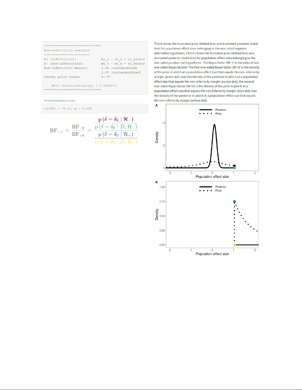
BA YMEDR 1 ba ymedr: An R P ac kage and W eb Application for the Calculation of Ba y es F actors for Superiority , Equiv alence, and Non-Inferiority Designs Maximilian Linde 1 and Don v an Ra v enzwaaij 1 1 Unit of Psyc hometrics and Statistics, Departmen t of Psychology , F acult y of Behavioural and So cial Sciences, Univ ersit y of Groningen, Groningen, The Netherlands A uthor Note Maximilian Linde h ttps://orcid.org/0000-0001-8421-090X Don v an Ra v enzwaaij h ttps://orcid.org/0000-0002-5030-4091 This researc h w as supp orted by a Dutc h scientific organization VIDI fello wship gran t a warded to Don v an Rav enzwaaij (016.Vidi.188.001). Corresp ondence concerning this article should b e addressed to: Maximilian Linde, Universit y of Groningen, Departmen t of Psyc hology , Grote Kruisstraat 2/1, Heymans Building, ro om 217, 9712 TS Groningen, The Netherlands, Phone: (+31) 50 363 2702, E-mail: m.linde@rug.nl BA YMEDR 2 Abstract Clinical trials often seek to determine the sup eriorit y , equiv alence, or non-inferiorit y of an exp erimen tal condition (e.g., a new drug) compared to a con trol condition (e.g., a placeb o or an already existing drug). The use of frequentist statistical metho ds to analyze data for these t yp es of designs is ubiquitous ev en though they hav e several limitations. Ba y esian inference remedies man y of these shortcomings and allo ws for intuitiv e interpretations. In this article, w e outline the frequen tist conceptualization of sup eriority , equiv alence, and non-inferiorit y designs and discuss its disadv an tages. Subsequen tly , w e explain how Ba yes factors can b e used to compare the relativ e plausibilit y of comp eting hypotheses. W e presen t ba ymedr, an R package and w eb application, that provides user-friendly tools for the computation of Ba y es factors for sup eriority , equiv alence, and non-inferiorit y designs. Instructions on ho w to use ba ymedr are provided and an example illustrates ho w already existing results can b e reanalyzed with ba ymedr. K eywor ds: Ba y es factor, baymedr, equiv alence, non-inferiority , sup eriorit y BA YMEDR 3 ba ymedr: An R P ac kage and W eb Application for the Calculation of Ba y es F actors for Sup eriority , Equiv alence, and Non-Inferiority Designs In tro duction Researc hers generally agree that the clinical trial is the b est metho d to determine and compare the effects of medications and treatmen ts (E. Christensen, 2007; F riedman et al., 2010). Although clinical trials are often similar in design, differen t statistical pro cedures need to b e emplo y ed dep ending on the nature of the research question. Commonly , clinical trials seek to determine the sup eriorit y , equiv alence, or non-inferiorit y of an exp erimen tal condition (e.g., sub jects receiving a new medication) compared to a con trol condition (e.g., sub jects receiving a placeb o or an already existing medication; Lesaffre, 2008; Piaggio et al., 2012). F or these goals, statistical inference is often conducted in the form of testing. Usually , the frequen tist approach to statistical testing forms the framework in whic h data for these researc h designs are analyzed (Cha v alarias et al., 2016). In particular, researc hers often rely on n ull hypothesis significance testing (NHST), which quantifies evidence through a p -v alue. This p -v alue represents the probability of obtaining a test statistic (e.g., a t -v alue) at least as extreme as the one observ ed, assuming that the null h yp othesis is true. In other words, the p -v alue is an indicator of the unusualness of the obtained test statistic under the n ull h yp othesis, forming a “pro of by con tradiction” (R. Christensen, 2005, p. 123). If the p -v alue is smaller than a predefined T yp e I error rate ( α ), typically set to α = . 05 (but see, e.g., Benjamin et al., 2018; Lak ens, Adolfi, et al., 2018), rejection of the n ull h yp othesis is warran ted; otherwise the obtained data do not justify rejection of the n ull h yp othesis. The NHST approac h to inference has b een criticized due to certain limitations and erroneous in terpretations of p -v alues (e.g., Berger & Sellk e, 1987; Cohen, 1994; Dienes, 2011; Gigerenzer et al., 2004; Go o dman, 1999a, 1999b, 2008; Loftus, 1996; v an Ra v enzw aaij & Ioannidis, 2017; W agenmak ers, 2007; W agenmak ers et al., 2018; W asserstein & Lazar, BA YMEDR 4 2016; W etzels et al., 2011), whic h w e briefly describ e b elow. As a result, some metho dologists ha v e argued that p -v alues should b e mostly abandoned from scientific practice (e.g., Berger & Delampady, 1987; Go o dman, 2008; McShane et al., 2019; W agenmak ers et al., 2018). An alternativ e to NHST is statistical testing within a Bay esian framew ork. Ba y esian statistics is based on the idea that the credibilities of well-defined parameter v alues (e.g., effect size) or mo dels (e.g., n ull and alternativ e hypotheses) are up dated based on new observ ations (Krusc hk e, 2015). With explo ding computational p o w er and the rise of Mark o v chain Mon te Carlo metho ds (e.g., Gilks et al., 1995; v an Rav enzwaaij et al., 2018) that are used to estimate probabilit y distributions that cannot b e determined analytically , applications of Ba y esian inference hav e recently b ecome tractable. Indeed, Ba y esian metho ds are seeing more and more use in the biomedical field (Berry, 2006) and other disciplines (v an de Sc ho ot et al., 2017). Despite the fact that statistical inference is slo wly c hanging from frequentist metho ds to w ards Bay esian metho ds, a ma jorit y of biomedical research still employs frequen tist statistical tec hniques (Chav alarias et al., 2016). T o some exten t, this migh t b e due to a biased statistical education in fa v or of frequentist inference. Moreo v er, researc hers migh t p erceiv e statistical inference through NHST and rep orting of p -v alues as prescriptive and, hence, adhere to this con v ention (Gigerenzer, 2004; Winkler, 2001). W e b eliev e that one of the most crucial factors is the una v ailabilit y of easy-to-use Bay esian to ols and soft w are, leaving Ba yesian h yp othesis testing largely to statistical exp erts. F ortunately , imp ortan t adv ances ha ve b een made to wards user-friendly in terfaces for Bay esian analyses with the release of the Ba y esF actor softw are (Morey & Rouder, 2018), written in R (R Core T eam, 2021), and p oin t-and-clic k softw are like JASP (JASP T eam, 2021) and Jamovi (The jamo vi pro ject, 2021), the latter t wo of whic h are based to some extent on the Ba y esF actor softw are. Ho w ev er, these to ols are mainly tailored tow ards research designs in the so cial sciences. Easy-to-use Bay esian to ols and corresp onding accessible softw are for BA YMEDR 5 the analysis of biomedical researc h designs sp ecifically (e.g., sup eriorit y , equiv alence, and non-inferiorit y) are still missing and, th us, urgently needed. In this article, w e pro vide a softw are package and a web application for conducting Ba y esian hypothesis tests for sup eriority , equiv alence, and non-inferiorit y designs. Although implemen tations for the sup eriorit y and equiv alence test exist elsewhere, the implemen tation of the non-inferiorit y test is nov el. Firstly , w e outline the traditional frequen tist approac h to statistical testing for each of these designs. Secondly , w e discuss the k ey disadv an tages and p otential pitfalls of this approac h and motiv ate why Bay esian inferen tial tec hniques are b etter suited for these research designs. Thirdly , w e explain the conceptual bac kground of Ba yes factors (Go o dman, 1999b; Jeffreys, 1939, 1948, 1961; Kass & Raftery, 1995). F ourthly , we provide and introduce baymedr (Linde & v an Rav enzwaaij, 2021), an op en-source softw are written in R (R Core T eam, 2021) that comes together with a web application (h ttps://maxlinde.shin yapps.io/ba ymedr/), for the computation of Ba y es factors for common biomedical designs. W e pro vide step-by-step instructions on how to use ba ymedr. Finally , we present a reanalysis of an existing empirical study to illustrate the most imp ortant features of the baymedr R pac kage and the accompanying w eb application. F requentist Inference for Sup eriority , Equiv alence, and Non-Inferiority Designs The sup eriorit y , equiv alence, and non-inferiorit y tests are concerned with research settings in whic h t wo conditions (e.g., con trol and exp erimental) are compared on some outcome measure (E. Christensen, 2007; Lesaffre, 2008). F or instance, researc hers migh t w an t to inv estigate whether a new antidepressan t medication is sup erior, equiv alent, or non-inferior compared to a w ell-established an tidepressant. F or a con tin uous outcome v ariable, the b et w een-group comparison is typically made with one or t wo t -tests. The three designs differ, ho w ever, in the precise sp ecification of the t -tests (see Fig 1). In the follo wing, w e will assume that higher scores on the outcome measure of in terest represen t a more fav orable outcome (i.e., sup eriority or non-inferiorit y) than low er scores. F or example, high scores are fav orable when the measure of in terest represen ts the BA YMEDR 6 n um b er of so cial interactions in patien ts with so cial anxiety , whereas lo w scores are fa v orable when the outcome v ariable is the num b er of depressive symptoms in patien ts with ma jor depressiv e disorder. W e will also assume that the outcome v ariable is con tin uous and that the residuals within b oth conditions are Normal distributed in the p opulation, sharing a common p opulation v ariance. Throughout this article, the true p opulation effect size ( δ ) reflects the true standardized difference in the outcome b etw een the exp erimen tal condition (i.e., e) and the con trol condition (i.e., c): δ = µ e − µ c σ . (1) The Sup eriorit y Design The sup eriorit y design tests whether the exp erimen tal condition is sup erior to the con trol condition (see the first ro w of Fig 1). Conceptually , the sup eriorit y design consists of a one-sided test due to its inherent directionalit y . The null h yp othesis H 0 states that the true p opulation effect size is zero, whereas the alternativ e h yp otheses H 1 states that the true p opulation effect size is larger than zero: H 0 : δ = 0 H 1 : δ > 0 . (2) T o test these h yp otheses, a one-sided t -test is conducted. 1 The Equiv alence Design The equiv alence design tests whether the exp erimen tal and con trol conditions are practically equiv alen t (see the second ro w of Fig 1). There are m ultiple approac hes to equiv alence testing (see, e.g., Meyners, 2012). A comprehensive treatmen t of all approaches is b ey ond the scop e of this article. Here, we fo cus on one p opular alternative: the tw o 1 Researc hers often conduct a t wo-sided t -test and then confirm that the observed effect go es in the exp ected direction. W e do not describ e this approach because w e hav e the opinion that a one-sided t -test should b e conducted for the superiority test, whose name already implies a uni-directional alternative h yp othesis. BA YMEDR 7 N on- superiorit y Superiorit y N on-equiv alenc e E quiv alenc e N on-equiv alenc e Inf eriorit y N on-inf eriorit y − c 0 c δ Figure 1 Schematic depiction of the sup eriority, e quivalenc e, and non-inferiority designs. The x -axis r epr esents the true p opulation effe ct size ( δ ), wher e c is the standar dize d e quivalenc e mar gin in c ase of the e quivalenc e test and the standar dize d non-inferiority mar gin in c ase of the non-inferiority test. Gr ay r e gions mark the nul l hyp otheses and white r e gions the alternative hyp otheses. The r e gion with the diagonal black lines is not use d for the one-side d sup eriority design. Note that the diagr am assumes that high values on the me asur e of inter est r epr esent sup erior or non-inferior values and that a one-side d test is use d for the sup eriority design. one-sided tests pro cedure (TOST; Ho dges & Lehmann, 1954; Sc h uirmann, 1987; W estlake, 1976; see also Meyners, 2012; Senn, 2008). An equiv alence interv al must b e defined, which BA YMEDR 8 can b e based, for example, on the smallest effect size of in terest (Lakens, 2017; Lak ens, Sc heel, et al., 2018). The sp ecification of the equiv alence interv al is not a statistical question; th us, it should b e set b y exp erts in the resp ective fields (Meyners, 2012; Sc h uirmann, 1987) or comply with regulatory guidelines (Garrett, 2003). Imp ortan tly , ho w ever, the equiv alence in terv al should b e determined indep endent of the obtained data. TOST in v olves conducting t wo one-sided t -tests, each one with its o wn null and alternativ e h yp otheses. F or the first test, the n ull h yp othesis states that the true p opulation effect size is smaller than the lo w er b oundary of the equiv alence interv al, whereas the alternativ e h yp othesis states that the true p opulation effect size is larger than the lo w er b oundary of the equiv alence interv al. F or the second test, the n ull h yp othesis states that the true p opulation effect size is larger than the upp er b oundary of the equiv alence in terv al, whereas the alternativ e hypothesis states that the true p opulation effect size is smaller than the upp er b oundary of the equiv alence in terv al. Assuming that the equiv alence in terv al is symmetric around the n ull v alue, these hypotheses can b e summarized as follo ws: H 0 : δ ≤ − c OR δ ≥ c H 1 : δ > − c AND δ < c , (3) where c represen ts the margin of the standardized equiv alence in terv al. T w o p -v alues ( p − c and p c ) result from the application of the TOST pro cedure. W e reject the n ull h yp othesis of non-equiv alence and, th us, establish equiv alence if max ( p − c , p c ) < α (cf. Meyners, 2012; W alk er & No wac ki, 2011). In other w ords, b oth tests need to reac h statistical significance. The Non-Inferiorit y Design In some situations, researc hers are in terested in testing whether the exp erimental condition is non-inferior or not w orse than the con trol condition by a certain amount. This is the goal of the non-inferiorit y design, whic h consists of a one-tailed test (see the third ro w of Fig 1). Realistic applications migh t include testing the effectiv eness of a new medication that has few er undesirable adv erse effects (Chadwick & Vigabatrin Europ ean BA YMEDR 9 Monotherap y Study Group, 1999), is c heap er (Kaul & Diamond, 2006), or is easier to administer than the curren t medication (V an de W erf et al., 1999). In these cases, w e need to p onder the cost of a somewhat lo w er or equal effectiveness of the new treatment with the v alue of the just men tioned b enefits (Hills, 2017). The n ull h yp othesis states that the true p opulation effect size is equal to a predetermined threshold, whereas the alternativ e h yp othesis states that the true p opulation effect size is higher than this threshold: H 0 : δ = − c H 1 : δ > − c , (4) where c represen ts the standardized non-inferiorit y margin. As with the equiv alence in terv al, the non-inferiorit y margin should b e defined indep endent of the obtained data. Limitations of F requentist Inference T ests of sup eriorit y , equiv alence, and non-inferiorit y hav e great v alue in biomedical researc h. It is the wa y researchers conduct their statistical analyses that, we argue, should b e critically reconsidered. There are several disadv antages asso ciated with the application of NHST to sup eriorit y , equiv alence, and non-inferiorit y designs. Here, w e limit our discussion to tw o disadv an tages; for a more comprehensiv e exp osition we refer the reader to other sources (e.g., Go o dman, 1999a; In ternational Committee of Medical Journal Editors, 1997; Rennie, 1978; W agenmak ers et al., 2018). First, researc hers need to stic k to a predetermined sampling plan (Rouder, 2014; Sc hön bro dt & W agenmak ers, 2018; Sc hön bro dt et al., 2017). That is, it is not legitimate to decide based on in terim results to stop data collection (e.g., b ecause the p -v alue is already smaller than α ) or to contin ue data collection b eyond the predetermined sample size (e.g., b ecause the p -v alue almost reac hes statistical significance). In principle, researchers can correct for the fact that they insp ected the data b y reducing the required significance threshold through one of sev eral tec hniques (Ranganathan et al., 2016). Ho w ever, suc h correction metho ds are rarely applied. Esp ecially in biomedical research, the p ossibility of optional stopping could reduce the w aste of resources for exp ensiv e and time-consuming BA YMEDR 10 trials (Chalmers & Glasziou, 2009). Second, with the traditional frequen tist framew ork it is imp ossible to quantify evidence in fa v or of the null h yp othesis (Gallistel, 2009; Rouder et al., 2009; v an Ra v enzwaaij et al., 2019; W agenmak ers, 2007; W agenmakers et al., 2018). Often times, the p -v alue is erroneously in terpreted as a p osterior probabilit y , in the sense that it represents the probabilit y of the n ull hypothesis (Berger & Sellke, 1987; Gelman, 2013; Go o dman, 2008; Haller & Krauss, 2002). How ever, a non-significant p -v alue do es not only o ccur when the null h yp othesis is in fact true but also when the alternativ e hypothesis is true, yet there w as not enough p o wer to detect an effect (Bakan, 1966; v an Ra venzw aaij et al., 2019). As Altman and Bland (1995, p. 485) put it: “Absence of evidence is not evidence of absence” . Still, a large prop ortion of biomedical studies falsely claim equiv alence based on statistically non-significan t t -tests (Greene et al., 2000). Y et, estimating evidence in fa v or of the n ull h yp othesis is essential for certain designs lik e the equiv alence test (Blackw elder, 1982; Ho ekstra et al., 2018; v an Ra v enzwaaij et al., 2019). The TOST pro cedure for equiv alence testing pro vides a workaround for the problem that evidence for the n ull h yp othesis cannot b e quantified with frequen tist techniques by defining an equiv alence in terv al around δ = 0 and conducting tw o tests. Without this in terv al the TOST pro cedure w ould inevitably fail (see Meyners, 2012, for an explanation of wh y this is the case). As w e will see, the Ba y esian equiv alence test do es not hav e this restriction; it allo ws for the sp ecification of in terv al as well as p oin t null hypotheses. Ba y esian T ests for Sup eriority , Equiv alence, and Non-Inferiority Designs The Ba y esian statistical framework pro vides a logically sound metho d to up date b eliefs ab out parameters based on new data (Go o dman, 1999b; Krusc hk e, 2015). Ba y esian inference can b e divided in to parameter estimation (e.g., estimating a p opulation correlation) and mo del comparison (e.g., comparing the relativ e probabilities of the data under the n ull and alternativ e hypotheses) pro cedures (see, e.g., Kruschk e & Liddell, 2018b, for an o v erview). Here, w e will fo cus on the latter approac h, which is usually BA YMEDR 11 accomplished with Ba y es factors (Go o dman, 1999b; Jeffreys, 1939, 1948, 1961; Kass & Raftery, 1995). In our exp osition of Bay es factors in general and sp ecifically for sup eriority , equiv alence, and non-inferiorit y designs, w e mostly refrain from complex equations and deriv ations. F ormulas are only provided when we think that they help to communicate the ideas and concepts. W e refer readers interested in the mathematics of Bay es factors to other sources (e.g., Etz & V andek erc khov e, 2018; Jeffreys, 1961; Kass & Raftery, 1995; O’Hagan & F orster, 2004; Rouder et al., 2009; W agenmak ers et al., 2010). The precise deriv ation of Ba y es factors for sup eriority , equiv alence, and non-inferiorit y designs in particular is treated elsewhere (v an Ra v enzwaaij et al., 2019; see also Gronau et al., 2020). The Ba y es F actor Let us supp ose that w e ha ve t wo h yp otheses, H 0 and H 1 , that w e w ant to con trast. Without considering an y data, w e hav e initial b eliefs ab out the probabilities of H 0 and H 1 , whic h are giv en by the prior probabilities p ( H 0 ) and p ( H 1 ) = 1 − p ( H 0 ) . Now, we collect some data D . After having seen the data, we hav e new and refined b eliefs ab out the probabilities that H 0 and H 1 are true, whic h are giv en by the p osterior probabilities p ( H 0 | D ) and p ( H 1 | D ) = 1 − p ( H 0 | D ) . In other w ords, we up date our prior b eliefs ab out the probabilities of H 0 and H 1 b y incorp orating what the data dictates w e should b eliev e and arriv e at our p osterior b eliefs. This relation is expressed in Ba y es’ rule: p ( H i | D ) | {z } Posterior = Likelihood z }| { p ( D | H i ) Prior z }| { p ( H i ) p ( D | H 0 ) p ( H 0 ) + p ( D | H 1 ) p ( H 1 ) | {z } Marginal Likelihoo d , (5) with i = { 0 , 1 } , and where p ( H i ) represen ts the prior probabilit y of H i , p ( D | H i ) denotes the lik eliho o d of the data under H i , p ( D | H 0 ) p ( H 0 ) + p ( D | H 1 ) p ( H 1 ) is the marginal lik eliho o d (also called evidence; Krusc hk e, 2015), and p ( H i | D ) is the p osterior probabilit y of H i . As we will see, the likelihoo d in Equation 5 is actually a marginal lik eliho o d b ecause eac h mo del (i.e., H 0 and H 1 ) con tains certain parameters that are in tegrated out. The BA YMEDR 12 denominator in Equation 5 (lab eled marginal lik eliho o d) serv es as a normalization constan t, ensuring that the sum of the p osterior probabilities is 1. Without this normalization constan t the p osterior is still prop ortional to the pro duct of the lik eliho o d and the prior. Therefore, for H 0 and H 1 w e can also write: p ( H i | D ) ∝ p ( D | H i ) p ( H i ) , (6) where ∝ means “is prop ortional to” . Rather than using p osterior probabilities for eac h h yp othesis, let the ratio of the p osterior probabilities for H 0 and H 1 b e: p ( H 0 | D ) p ( H 1 | D ) | {z } Posterior odds = p ( D | H 0 ) p ( D | H 1 ) | {z } Bay es factor, BF 01 p ( H 0 ) p ( H 1 ) | {z } Prior o dds . (7) The quan tit y p ( H 0 | D ) /p ( H 1 | D ) represents the p osterior o dds and the quantit y p ( H 0 ) /p ( H 1 ) is called the prior o dds. T o get the p osterior o dds, we hav e to multiply the prior o dds with p ( D | H 0 ) /p ( D | H 1 ) , a quan tit y known as the Ba yes factor (Go o dman, 1999b; Jeffreys, 1939, 1948, 1961; Kass & Raftery, 1995), whic h is a ratio of marginal lik eliho o ds: BF 01 = R θ 0 p ( D | θ 0 , H 0 ) p ( θ 0 | H 0 ) d θ 0 R θ 1 p ( D | θ 1 , H 1 ) p ( θ 1 | H 1 ) d θ 1 , (8) where θ 0 and θ 1 are v ectors of parameters under H 0 and H 1 , resp ectiv ely . In other words, the marginal lik eliho o ds in the n umerator and denominator of Equation 8 are weigh ted a v erages of the likelihoo ds, for which the w eights are determined by the corresp onding prior. In the case where one hypothesis has fixed v alues for the parameter v ector θ i (e.g., a p oin t n ull h yp othesis), in tegration o v er the parameter space and the sp ecification of a prior is not required. In that case, the marginal likelihoo d b ecomes a likelihoo d. The Ba y es factor is the amount b y which we w ould up date our prior o dds to obtain the p osterior o dds, after taking in to consideration the data. F or example, if we had prior o dds of 2 and the Ba y es factor is 24, then the p osterior o dds would b e 48. In the sp ecial case where the prior o dds is 1, the Ba y es factor is equal to the p osterior o dds. A ma jor BA YMEDR 13 adv an tage of the Ba yes factor is its ease of interpretation. F or example, if the Ba y es factor (BF 01 , denoting the fact that H 0 is in the n umerator and H 1 in the denominator) equals 10, the data are ten times more lik ely to hav e o ccurred under H 0 compared to H 1 . With BF 01 = 0 . 2 , we can say that the data are five times more likely under H 1 compared to H 0 b ecause w e can simply tak e the recipro cal of BF 01 (i.e., BF 10 = 1 / BF 01 ). What constitutes enough evidence is sub jectiv e and certainly dep ends on the con text. Nev ertheless, rules of th um b for evidence thresholds hav e b een prop osed. F or instance, Kass and Raftery (1995) lab eled Ba y es factors b etw een 1 and 3 as “not worth more than a bare mention”, Ba yes factors b et ween 3 and 20 as “p ositive”, those b et w een 20 and 150 as “strong”, and an ything ab o v e 150 as “very strong”, with corresp onding thresholds for the recipro cals of the Ba yes factors. An alternative classification scheme was already prop osed b efore, with thresholds at 3, 10, 30, and 100 and similar lab els (Jeffreys, 1961; see also Lee & W agenmak ers, 2013, for up dated lab els). Of course, w e need to define H 0 and H 1 . In other words, b oth mo dels contain certain parameters for whic h w e need to determine a prior distribution. Here, w e will assume that the residuals of the t w o groups are Normal distributed in the p opulation with a common p opulation v ariance. The shap e of a Normal distribution is fully determined with the lo cation (mean; µ ) and the scale (v ariance; σ 2 ) parameters. Thus, in principle, b oth mo dels con tain t wo parameters. No w, w e mak e tw o imp ortan t changes. Firstly , in the case where w e ha ve a p oin t null hypothesis, µ under H 0 is fixed at δ = 0 , leaving σ 2 for H 0 and µ and σ 2 for H 1 . Parameter σ 2 is a n uisance parameter b ecause it is common to b oth mo dels. Placing a Jeffreys prior (also called right Haar prior), p ( σ 2 ) ∝ 1 /σ 2 , on this n uisance parameter (Gönen et al., 2005; Gronau et al., 2020; Jeffreys, 1961) has sev eral desirable prop erties that are explained elsewhere (e.g., Ba yarri et al., 2012; Berger et al., 1998). Secondly , µ under H 1 can b e expressed in terms of a p opulation effect size δ (Gönen et al., 2005; Rouder et al., 2009). This establishes a common and comparable scale across BA YMEDR 14 exp erimen ts and p opulations (Rouder et al., 2009). The prior on δ could reflect certain h yp otheses that w e wan t to test. F or instance, w e could compare the n ull hypothesis ( H 0 : δ = 0 ) to a tw o-sided alternative hypotheses ( H 1 : δ 6 = 0 ) or to one of tw o one-sided alternativ e h yp otheses ( H 1 : δ < 0 or H 1 : δ > 0 ). Alternatively , w e could compare an in terv al h yp othesis for the null h yp othesis ( H 0 : − c < δ < c ) with a corresp onding alternativ e h yp othesis ( H 1 : δ < − c OR δ > c ). 2 The c hoice of the sp ecific prior for δ is a delicate matter, whic h is discussed in the next section. In the most general case, the Ba y es factor (i.e., BF 01 ) can b e calculated through division of the p osterior o dds b y the prior o dds (i.e., rearranging Equation 7): BF 01 = p ( H 0 | D ) p ( H 1 | D ) ! p ( H 0 ) p ( H 1 ) ! = p ( H 0 | D ) p ( H 0 ) ! p ( H 1 | D ) p ( H 1 ) ! ; (9) accordingly , w e can also calculate BF 10 : BF 10 = p ( H 1 | D ) p ( H 0 | D ) ! p ( H 1 ) p ( H 0 ) ! = p ( H 1 | D ) p ( H 1 ) ! p ( H 0 | D ) p ( H 0 ) ! . (10) Calculating Ba y es factors this wa y often inv olves solving complex in tegrals (see, e.g., Equation 8; also cf. W agenmak ers et al., 2010). F ortunately , there is a computational shortcut for the sp ecific but v ery common scenario where w e hav e a p oint n ull hypothesis and a complemen tary in terv al alternative h yp othesis. This shortcut, whic h is called the Sa v age-Dic key densit y ratio, takes the ratio of the density of the prior and p osterior at the n ull v alue under the alternativ e hypothesis to calculate the Bay es factor; this is explained in more detail elsewhere (Dick ey & Lientz, 1970; Kass & Raftery, 1995; v an Rav enzwaaij & Etz, 2021; W agenmak ers et al., 2010). 2 Note that the hypotheses represent exactly the opposite of the hypotheses in TOST (i.e., H 0 of equiv alence corresp onds to H 1 of equiv alence in TOST, and vice versa). Evidence in fa vor of equiv alence in TOST can only b e obtained b y rejecting tw o n ull h yp otheses: H 0 : δ < − c and H 0 : δ > c . F or the Bay esian equiv alence test w e use the more intuitiv e null hypothesis of equiv alence (i.e., H 0 : − c < δ < c ). BA YMEDR 15 Default Priors Un til this p oin t in our exp osition, we w ere quite v ague ab out the form of the prior for δ under H 1 . In principle, the prior for δ within H 1 can b e defined as desired, conforming to the b eliefs of the researc her. In fact, this is a fundamen tal part of Ba yesian inference b ecause v arious priors allo w for the expression of a theory or prior b eliefs (Morey et al., 2016; V anpaemel, 2010). Most commonly , ho w ever, default or ob jectiv e priors are emplo y ed that aim to increase the ob jectivity in sp ecifying the prior or serv e as a default when no sp ecific prior information is a v ailable (Consonni et al., 2018; Jeffreys, 1961; Rouder et al., 2009). W e employ ob jective priors in baymedr. In the situation where we ha ve a p oin t null h yp othesis and an alternative h yp othesis that in v olves a range of v alues, Jeffreys (1961) prop osed to use a Cauch y prior with a scale parameter of r = 1 for δ under H 1 . This Cauch y distribution is equiv alent to a Student’s t distribution with 1 degree of freedom and resembles a standard Normal distribution, except that the Cauc h y distribution has less mass at the center but instead hea vier tails (see Fig 2; Rouder et al., 2009). Mathematically , the Cauch y distribution corresp onds to the com bined sp ecification of (1) a Normal prior with mean µ δ and v ariance σ 2 δ on δ ; and (2) an inv erse Chi-square distribution with 1 degree of freedom on σ 2 δ . Integrating out σ 2 δ yields the Cauc h y distribution (Liang et al., 2008; Rouder et al., 2009). The scale parameter r defines the width of the Cauc h y distribution; that is, half of the mass lies b etw een − r and r . Cho osing a Cauc h y prior with a lo cation parameter of 0 and a scale parameter of r = 1 has the adv antage that the resulting Bay es factor is 1 in case of completely uninformativ e data. In turn, the Bay es factor approaches infinity (or 0 ) for decisive data (Ba y arri et al., 2012; Jeffreys, 1961). Still, b y v arying the Cauc hy scale parameter, w e can set a differen t emphasis on the prior credibilit y of a range of effect sizes. More recen tly , a Cauc h y prior scale of r = 1 / √ 2 is used as a default setting in the Ba yesF actor soft ware (Morey & Rouder, 2018), the p oin t-and-clic k softw are JASP (JASP T eam, 2021), and Jamo vi (The jamo vi pro ject, 2021). W e ha v e adopted this v alue in baymedr as a default BA YMEDR 16 0 0.1 0.2 0.3 0.4 0.5 -4 -3 -2 -1 0 1 2 3 4 δ D ensit y S tand ard Normal S tand ard C auch y Figure 2 Comp arison of the standar d Normal pr ob ability density function (solid line) and the standar d Cauchy pr ob ability density function (dashe d line). setting. Nevertheless, ob jective priors are often criticized (see, e.g., Kruschk e & Liddell, 2018a; T endeiro & Kiers, 2019); researc hers are encouraged to use more informed priors if relev an t kno wledge is av ailable (Gronau et al., 2020; Rouder et al., 2009). Using ba ymedr With the ba ymedr soft ware (BA Y esian inference for MEDical designs in R; Linde & v an Ra v enzwaaij, 2021), written in R (R Core T eam, 2021), and the corresp onding web application (accessible at h ttps://maxlinde.shin yapps.io/ba ymedr/) one can easily calculate Ba y es factors for sup eriority , equiv alence, and non-inferiorit y designs. The R BA YMEDR 17 pac kage can b e used b y researchers who ha ve only rudimentary kno wledge of R; if that is not the case, researc hers can use the w eb application, which do es not require any kno wledge of programming. In the following, we will demonstrate how Bay es factors for sup eriorit y , equiv alence, and non-inferiorit y designs can b e calculated with the baymedr R pac kage; a thorough explanation of the w eb application is not necessary as it strongly o v erlaps with the R package. Subsequen tly , w e will show case (1) the baymedr R pac kage and (2) the corresp onding w eb application b y reanalyzing data of an empirical study by Basner et al. (2019). The R P ac kage Instal l and L o ad b ayme dr T o install the latest release of the ba ymedr R package from The Comprehensiv e R Arc hiv e Netw ork (CRAN; https://CRAN.R-project.org/package=ba ymedr), use the follo wing command: install.packages("baymedr") The most recen t v ersion of the R package can b e obtained from GitHub (h ttps://gith ub.com/maxlinde/baymedr) with the help of the devto ols pac kage (Wickham et al., 2019): devtools::install_github("maxlinde/baymedr") Once ba ymedr is installed, it needs to b e loaded in to memory , after which it is ready for usage: library("baymedr") Commonalities A cr oss Designs F or all three researc h designs, the user has three options for data input (function argumen ts that ha ve “x” as a name or suffix refer to the control condition and those with “y” as a name or suffix to the exp erimen tal condition): (1) pro vide the ra w data; the BA YMEDR 18 relev an t argumen ts are x and y ; (2) provide the sample sizes, sample means, and sample standard deviations; the relev an t argumen ts are n_x and n_y for sample sizes, mean_x and mean_y for sample means, and sd_x and sd_y for sample standard deviations; (3) pro vide the sample sizes, sample means, and the confidence in terv al for the difference in group means; the relev an t argumen ts are n_x and n_y for sample sizes, mean_x and mean_y for sample means, and ci_margin for the confidence in terv al margin and ci_level for the confidence lev el. The Cauc h y distribution is used as the prior for δ under the alternativ e h yp othesis for all three tests. The user can set the width of the Cauc h y prior with the prior_scale argumen t, th us, allowing the sp ecification of differen t ranges of plausible effect sizes. In all three cases, the Cauc h y prior is centered on δ = 0 . F urther, ba ymedr uses a default Cauch y prior scale of r = 1 / √ 2 , complying with the standard settings of the Ba y esF actor softw are (Morey & Rouder, 2018), JASP (JASP T eam, 2021), and Jamo vi (The jamovi pro ject, 2021). Once a sup eriorit y , equiv alence, or non-inferiorit y test is conducted, an informative and accessible output message is prin ted in the console. F or all three designs, this output states the t yp e of test that w as conducted and whether raw or summary data were used. Moreo v er, the corresp onding null and alternativ e hypotheses are restated and the sp ecified Cauc h y prior scale is shown. In addition, the lo w er and upp er b ounds of the equiv alence in terv al are presen ted in case an equiv alence test was emplo yed; similarly , the non-inferiorit y margin is prin ted when the non-inferiority design was c hosen. Lastly , the resulting Ba y es factor is shown. T o a v oid any confusion, it is declared in brack ets whether the Ba y es factor quantifies evidence to wards the null (e.g., equiv alence) or alternativ e (e.g., non-inferiorit y or sup eriorit y) hypothesis. Conducting Sup eriority, Equivalenc e, and Non-inferiority T ests The Ba y esian sup eriority test is p erformed with the super_bf() function. Dep ending on the researc h setting, lo w or high scores on the measure of interest represent BA YMEDR 19 “sup eriorit y”, whic h is sp ecified by the argumen t direction . Since w e seek to find evidence for the alternativ e h yp othesis (sup eriority), the Ba yes factor quan tifies evidence for H 1 relativ e to H 0 (i.e., BF 10 ). The Ba y esian equiv alence test is done with the equiv_bf() function. The desired equiv alence in terv al is sp ecified with the interval argumen t. Sev eral options are p ossible: A symmetric equiv alence in terv al around δ = 0 can b e indicated by providing one v alue (e.g., interval = 0.2 ) or by pro viding a vector with the negativ e and the p ositive v alues (e.g., interval = c(-0.2, 0.2) ). An asymmetric equiv alence interv al can b e sp ecified by pro viding a v ector with the negative and the p ositiv e v alues (e.g., interval = c(-0.3, 0.2) ). The implementation of a p oint n ull hypothesis is achiev ed by using either interval = 0 or interval = c(0, 0) , whic h also serves as the default sp ecification. The argument interval_std can b e used to declare whether the equiv alence in terv al w as sp ecified in standardized or unstandardized units. Since w e seek to quan tify evidence to w ards equiv alence, we con trast the evidence for H 0 relativ e to H 1 (i.e., BF 01 ). The Ba y es factor for the non-inferiority design is calculated with the infer_bf() function. The v alue for the non-inferiority margin can b e sp ecified with the ni_margin argumen t. The argument ni_margin_std can b e used to declare whether the non-inferiorit y margin w as given in standardized or unstandardized units. Lastly , dep ending on whether high or lo w v alues on the measure of in terest represent “non-inferiorit y”, one of the options “high” or “lo w” should b e set for the argument direction . W e wish to determine the evidence in fav or of H 1 ; therefore, the evidence is expressed for H 1 relativ e to H 0 (i.e., BF 10 ). Demonstration of ba ymedr T o illustrate ho w the R pac kage and the web application can b e used, we pro vide one example of an empirical study that emplo y ed non-inferiority tests to inv estigate differences in the amoun t of sleep, sleepiness, and alertness among medical trainees follo wing either standard or flexible dut y-hour programs (Basner et al., 2019). The authors BA YMEDR 20 list sev eral disadv an tages of restricted duty-hour programs, suc h as: (1) “[t]ransitions [as a result of restricted dut y hours] in to and out of night shifts can result in fatigue from shift-w ork-related sleep loss and circadian misalignmen t”; (2) “[p]reven ting interns from participating in extended shifts ma y reduce educational opp ortunities”; (3) “increase[d] handoffs”; (4) “reduce[d] con tin uity of care”; and (5) “[r]estricting duty hours ma y increase the necessity of cross-cov erage, contributing to work compression for b oth interns and more senior residen ts” (Basner et al., 2019, p. 916). As outlined ab ov e, the calculation of Bay es factors for equiv alence and sup eriorit y tests is done quite similarly to the non-inferiorit y test, so w e do not pro vide sp ecific examples for those tests. F or the purp ose of this demonstration, w e will only consider the outcome v ariable sleepiness. P articipan ts w ere monitored o v er a p erio d of 14 days and w ere asked to indicate each morning ho w sleepy they w ere b y completing the Karolinska sleepiness scale (Åkerstedt & Gillb erg, 1990), a 9 -p oin t Lik ert scale ranging from 1 (extremely alert) to 9 (extremely sleepy , figh ting sleep). The dep endent v ariable consisted of the a v erage sleepiness score ov er the whole observ ation p erio d of 14 da ys. The research question was whether the flexible duty-hour program was non-inferior to the standard program in terms of sleepiness. The null h yp othesis w as that medical trainees in the flexible program are sleepier b y more than a non-inferiorit y margin than trainees in the standard program. Con v ersely , the alternativ e h yp othesis was that trainees in the flexible program are not sleepier by more than a non-inferiorit y margin than trainees in the standard program. The non-inferiorit y margin w as defined as 1 p oin t on the 9 -p oint Lik ert scale. All relev an t summary statistics can b e obtained or calculated from T able 1 and the Results section of Basner et al. (2019). T able 1 indicates that the flexible program had a mean of M e = 4 . 8 and the standard program had a mean of M c = 4 . 7 . F rom the Results section we can extract that sample sizes w ere n e = 205 and n c = 193 in the flexible and standard programs, resp ectively . F urther, the margin of the 95% CI of the difference b et ween the t wo conditions w as 0 . 31 − 0 . 12 = 0 . 19 . Finally , low er scores on the sleepiness scale constitute fav orable BA YMEDR 21 (non-inferior) outcomes. The R Package Using this information, w e can use the ba ymedr R package to calculate the Bay es factor as follo ws: infer_bf(n_x = 193, n_y = 205, mean_x = 4.7, mean_y = 4.8, ci_margin = 0.19, ci_level = 0.95, ni_margin = 1, ni_margin_std = FALSE, prior_scale = 1 / sqrt(2), direction = "low") Note that we decided to use a Cauc h y prior scale of r = 1 / √ 2 for this reanalysis. Since our Cauc h y prior scale of choice represen ts the default v alue in baymedr, it would not ha ve b een necessary to pro vide this argumen t; how ever, for purp oses of illustration, w e men tioned it explicitly in the function call. The output pro vides a user-friendly summary of the analysis: ****************************** Non-inferiority analysis ------------------------ Data: summary data H+ (inferiority): mu_y - mu_x > ni_margin H- (non-inferiority): mu_y - mu_x < ni_margin Non-inferiority margin: 1.04 (standardised) 1.00 (unstandardised) Cauchy prior scale: 0.707 BF-+ (non-inferiority) = 8.56e+10 BA YMEDR 22 ****************************** This large Ba y es factor supp orts the conclusion from Basner et al. (2019) that medical trainees in the flexible dut y-hour program are non-inferior in terms of sleepiness compared to medical trainees in the standard program ( p < . 001 ). In other words, the data are 8 . 56 × 10 10 more lik ely to ha ve o ccurred under H 1 than H 0 . The W eb Application Similarly , we can use the w eb application to calculate the Bay es factor. F or this, the w eb application should first b e op ened in a w eb browser (h ttps://maxlinde.shin yapps.io/ba ymedr/). The just-op ened w elcome page offers a brief description of the three researc h designs and Ba yes factors and lists several further useful resources for the in terested user. Since we wan t to conduct a non-inferiority test with summary data, w e clic k on “Non-inferiority” and then “Summary data” on the navigation bar at the top (see Fig 3). The summary statistics for the example reanalysis of Basner et al. (2019) can b e inserted in the corresp onding fields, as sho wn in Fig 3. F or some fields a small green question mark is sho wn, whic h provides more details and help when the user clic ks on them. F urthermore, the scale of the prior distribution can b e sp ecified, whic h b y default is set to 1 / sqrt(2) . A small dynamic plot accompanies the field for the Cauc h y prior scale. That is, once the prior scale is c hanged, the plot up dates automatically , so that users obtain an impression of what the distribution lo oks lik e and what effect sizes are included. Once the “Calculate Bay es factor” button is click ed, the output is displa y ed. Fig 4 sho ws the output of the calculations. The top of the left column displa ys the same output that is giv en with the R pac kage. F urther, up on clicking on “Show frequentist results”, the results of the frequen tist non-inferiorit y test are shown and clicking on “Hide frequen tist results” in turn hides those results. Belo w that output is the form ula for the Ba y es factor, with different elemen ts printed in colors that corresp ond to dots in matching colors in the plots on the righ t column of the results output. The upp er plot sho ws the prior and p osterior for con trasting H 0 : δ = c with H 1 : δ < c . The tw o distributions are BA YMEDR 23 Figure 3 Shown is p art of the b ayme dr web applic ation demonstr ating how summary statistics c an b e inserte d and further p ar ameters sp e cifie d for a Bayesian non-inferiority test. In this sp e cific c ase, the summary statistics c orr esp ond to the ones obtaine d fr om Basner et al. (2019). Se e text for details. truncated, meaning that they are cut off at δ = c . Similarly , the low er plot shows the truncated prior and p osterior for con trasting H 0 : δ = c with H 1 : δ > c . Through a heuristic called the Sa v age-Dic key densit y ratio (Dick ey & Lientz, 1970; Kass & Raftery, 1995; v an Ra v enzwaaij & Etz, 2021; W agenmakers et al., 2010), the ratio of the heights of the colored dots giv es us the Ba yes factor (see the colored expressions in the formula on the righ t side BA YMEDR 24 Figure 4 Shown is p art of the b ayme dr web applic ation showing the r esults of a Bayesian non-inferiority test. In this sp e cific c ase, the r esults c orr esp ond to a r e analysis using summary statistics obtaine d fr om Basner et al. (2019). Se e text for details. of the results output). The text ab ov e the tw o plots explains the plots as w ell. BA YMEDR 25 Discussion T ests of sup eriorit y , equiv alence, and non-inferiorit y are imp ortant means to compare the effectiv eness of medications and treatmen ts in biomedical research. Despite sev eral limitations, researc hers ov erwhelmingly rely on traditional frequentist inference to analyze the corresp onding data for these researc h designs (Cha v alarias et al., 2016). W e b eliev e that Ba yes factors (Go o dman, 1999b; Jeffreys, 1939, 1948, 1961; Kass & Raftery, 1995) are an attractiv e alternativ e to NHST and p -v alues b ecause they allow researc hers to quan tify evidence in fa vor of the n ull hypothesis (Gallistel, 2009; v an Rav enzwaaij et al., 2019; W agenmak ers, 2007; W agenmak ers et al., 2018) and p ermit sequential testing and optional stopping (Rouder, 2014; Sc hön bro dt & W agenmakers, 2018; Sc hönbrodt et al., 2017). In fact, we b elieve that the p ossibility for optional stopping and sequential testing has the p oten tial to largely reduce the w aste of scarce resources. This is esp ecially imp ortan t in the field of biomedicine, where clinical trials migh t b e exp ensive or ev en harmful for participan ts. Our ba ymedr R pac kage and web application (Linde & v an Rav enzw aaij, 2021) enable researc hers to conduct Ba yesian sup eriorit y , equiv alence, and non-inferiority tests. ba ymedr is c haracterized by a user-friendly implemen tation, making it conv enient for researc hers who are not statistical exp erts. F urthermore, using baymedr, it is p ossible to calculate Ba y es factors based on raw data and summary statistics, allowing for the reanalysis of published studies, for whic h the full data set is not av ailable. Comp eting in terests The authors declare no comp eting in terests. BA YMEDR 26 References Åk erstedt, T., & Gillb erg, M. (1990). Sub jectiv e and ob jective sleepiness in the activ e individual. International Journal of Neur oscienc e , 52 (1-2), 29–37. h ttps://doi.org/10.3109/00207459008994241 Altman, D. G., & Bland, J. M. (1995). Absence of evidence is not evidence of absence. BMJ , 311 (7003), 485–485. h ttps://doi.org/10.1136/bmj.311.7003.485 Bakan, D. (1966). The test of significance in psyc hological researc h. Psycholo gic al Bul letin , 66 (6), 423–437. h ttps://doi.org/10.1037/h0020412 Basner, M., Asch, D. A., Shea, J. A., Bellini, L. M., Carlin, M., Eck er, A. J., Malone, S. K., Desai, S. V., Sternberg, A. L., T onascia, J., Shade, D. M., Katz, J. T., Bates, D. W., Ev en-Shoshan, O., Silb er, J. H., Small, D. S., V olpp, K. G., Mott, C. G., Coats, S., . . . Dinges, D. F. (2019). Sleep and alertness in a dut y-hour flexibility trial in in ternal medicine. New England Journal of Me dicine , 380 (10), 915–923. h ttps://doi.org/10.1056/NEJMoa1810641 Ba y arri, M. J., Berger, J. O., F orte, A., & García-Donato, G. (2012). Criteria for Bay esian mo del c hoice with application to v ariable selection. The A nnals of Statistics , 40 (3), 1550–1577. h ttps://doi.org/10.1214/12- AOS1013 Benjamin, D. J., Berger, J. O., Johannesson, M., Nosek, B. A., W agenmak ers, E.-J., Berk, R., Bollen, K. A., Brem bs, B., Bro wn, L., Camerer, C., Cesarini, D., Cham b ers, C. D., Clyde, M., Co ok, T. D., De Bo ec k, P ., Dienes, Z., Dreb er, A., Easw aran, K., Efferson, C., . . . Johnson, V. E. (2018). Redefine statistical significance. Natur e Human Behaviour , 2 (1), 6–10. h ttps://doi.org/10.1038/s41562- 017- 0189- z Berger, J. O., & Delampady , M. (1987). T esting precise h yp otheses. Statistic al Scienc e , 2 (3), 317–335. h ttps://doi.org/10.1214/ss/1177013238 BA YMEDR 27 Berger, J. O., P ericc hi, L. R., & V arshavsky , J. A. (1998). Bay es factors and marginal distributions in in v arian t situations. Sankhy¯ a: The Indian Journal of Statistics , 60 , 307–321. Berger, J. O., & Sellk e, T. (1987). T esting a p oin t null h yp othesis: The irreconcilabilit y of p v alues and evidence. Journal of the A meric an Statistic al A sso ciation , 82 (397), 112–122. h ttps://doi.org/10.2307/2289131 Berry , D. A. (2006). Ba y esian clinical trials. Natur e R eviews Drug Disc overy , 5 (1), 27–36. h ttps://doi.org/10.1038/nrd1927 Blac kw elder, W. C. (1982). "proving the n ull hypothesis" in clinical trials. Contr ol le d Clinic al T rials , 3 (4), 345–353. https://doi.org/10.1016/0197- 2456(82)90024- 1 Chadwic k, D., & Vigabatrin Europ ean Monotherap y Study Group. (1999). Safety and efficacy of vigabatrin and carbamazepine in newly diagnosed epilepsy: A m ulticen tre randomised double-blind study. The L anc et , 354 (9172), 13–19. h ttps://doi.org/10.1016/S0140- 6736(98)10531- 7 Chalmers, I., & Glasziou, P . (2009). A v oidable w aste in the pro duction and rep orting of researc h evidence. The L anc et , 374 (9683), 86–89. h ttps://doi.org/10.1016/S0140- 6736(09)60329- 9 Cha v alarias, D., W allac h, J. D., Li, A. H. T., & Ioannidis, J. P . A. (2016). Evolution of rep orting p v alues in the biomedical literature, 1990-2015. Journal of the A meric an Me dic al A sso ciation , 315 (11), 1141–1148. https://doi.org/10.1001/jama.2016.1952 Christensen, E. (2007). Metho dology of sup eriorit y vs. equiv alence trials and non-inferiorit y trials. Journal of Hep atolo gy , 46 (5), 947–954. h ttps://doi.org/10.1016/j.jhep.2007.02.015 Christensen, R. (2005). T esting Fisher, Neyman, Pearson, and Ba y es. The A meric an Statistician , 59 (2), 121–126. h ttps://doi.org/10.1198/000313005X20871 Cohen, J. (1994). The earth is round (p < .05). A meric an Psycholo gist , 49 (12), 997–1003. h ttps://doi.org/10.1037/0003- 066X.49.12.997 BA YMEDR 28 Consonni, G., F ouskakis, D., Liseo, B., & Ntzoufras, I. (2018). Prior distributions for ob jectiv e Ba yesian analysis. Bayesian A nalysis , 13 (2), 627–679. h ttps://doi.org/10.1214/18- BA1103 Dic k ey , J. M., & Lientz, B. P . (1970). The weigh ted likelihoo d ratio, sharp hypotheses ab out c hances, the order of a Mark ov c hain. The A nnals of Mathematic al Statistics , 41 (1), 214–226. h ttps://doi.org/10.1214/aoms/1177697203 Dienes, Z. (2011). Ba y esian versus ortho do x statistics: Which side are you on? Persp e ctives on Psycholo gic al Scienc e , 6 (3), 274–290. https://doi.org/10.1177/1745691611406920 Etz, A., & V andek erc khov e, J. (2018). Introduction to Bay esian inference for psychology. Psychonomic Bul letin and R eview , 25 (1), 5–34. h ttps://doi.org/10.3758/s13423- 017- 1262- 3 F riedman, L. M., F urb erg, C. D., DeMets, D. L., Reb oussin, D. M., & Granger, C. B. (2010). F undamentals of clinic al trials (4th). Springer. Gallistel, C. R. (2009). The imp ortance of pro ving the n ull. Psycholo gic al R eview , 116 (2), 439–453. h ttps://doi.org/10.1037/a0015251 Garrett, A. D. (2003). Therap eutic equiv alence: F allacies and falsification. Statistics in Me dicine , 22 (5), 741–762. h ttps://doi.org/10.1002/sim.1360 Gelman, A. (2013). p v alues and statistical practice. Epidemiolo gy , 24 (1), 69–72. h ttps://doi.org/10.1097/EDE.0b013e31827886f7 Gigerenzer, G., Krauss, S., & Vitouch, O. (2004). The null ritual: What y ou alw ays w anted to kno w ab out significance testing but w ere afraid to ask. In D. Kaplan (Ed.), The sage handb o ok of quantitative metho dolo gy for the so cial scienc es (pp. 391–408). Sage. Gigerenzer, G. (2004). Mindless statistics. The Journal of So cio-Ec onomics , 33 (5), 587–606. h ttps://doi.org/10.1016/j.so cec.2004.09.033 Gilks, W. R., Ric hardson, S., & Spiegelhalter, D. (1995). Markov chain Monte Carlo in pr actic e . Chapman & Hall/CRC. BA YMEDR 29 Gönen, M., Johnson, W. O., Lu, Y., & W estfall, P . H. (2005). The Ba yesian t wo-sample t test. The A meric an Statistician , 59 (3), 252–257. h ttps://doi.org/10.1198/000313005X55233 Go o dman, S. N. (1999a). T o w ard evidence-based medical statistics. 1: The p v alue fallacy. A nnals of Internal Me dicine , 130 (12), 995–1004. h ttps://doi.org/10.7326/0003- 4819- 130- 12- 199906150- 00008 Go o dman, S. N. (1999b). T o w ard evidence-based medical statistics. 2: The Bay es factor. A nnals of Internal Me dicine , 130 (12), 1005–1013. h ttps://doi.org/10.7326/0003- 4819- 130- 12- 199906150- 00019 Go o dman, S. N. (2008). A dirt y dozen: T w elve p-v alue misconceptions. Seminars in Hematolo gy , 45 (3), 135–140. h ttps://doi.org/10.1053/j.seminhematol.2008.04.003 Greene, W. L., Concato, J., & F einstein, A. R. (2000). Claims of equiv alence in medical researc h: Are they supp orted b y the evidence? A nnals of Internal Me dicine , 132 (9), 715–722. h ttps://doi.org/10.7326/0003- 4819- 132- 9- 200005020- 00006 Gronau, Q. F., Ly , A., & W agenmak ers, E.-J. (2020). Informed Bay esian t-tests. The A meric an Statistician , 74 (2), 137–143. h ttps://doi.org/10.1080/00031305.2018.1562983 Haller, H., & Krauss, S. (2002). Misinterpretation of significance: A problem students share with their teac hers? Metho ds of Psycholo gic al R ese ar ch , 7 (1), 1–20. Hills, R. K. (2017). Non-inferiority trials: No b etter? no w orse? no change? no pain? British Journal of Haematolo gy , 176 (6), 883–887. https://doi.org/10.1111/bjh.14504 Ho dges, J. L., & Lehmann, E. L. (1954). T esting the appro ximate v alidit y of statistical h yp otheses. Journal of the R oyal Statistic al So ciety. Series B (Metho dolo gic al) , 16 (2), 261–268. Ho ekstra, R., Monden, R., v an Ra v enzwaaij, D., & W agenmak ers, E.-J. (2018). Bay esian reanalysis of n ull results rep orted in medicine: Strong y et v ariable evidence for the BA YMEDR 30 absence of treatmen t effects. PL oS ONE , 13 (4), e0195474. h ttps://doi.org/10.1371/journal.p one.0195474 In ternational Committee of Medical Journal Editors. (1997). Uniform requiremen ts for man uscripts submitted to biomedical journals. Patholo gy , 29 , 441–447. h ttps://doi.org/10.1080/00313029700169515 JASP T eam. (2021). JASP (V ersion 0.15)[Computer soft w are]. https://jasp- stats.org/ Jeffreys, H. (1939). The ory of pr ob ability . The Clarendon Press. Jeffreys, H. (1948). The ory of pr ob ability (2nd). The Clarendon Press. Jeffreys, H. (1961). The ory of pr ob ability (3rd). Oxford Universit y Press. Kass, R. E., & Raftery , A. E. (1995). Ba yes factors. Journal of the A meric an Statistic al A sso ciation , 90 (430), 773–795. h ttps://doi.org/10.2307/2291091 Kaul, S., & Diamond, G. A. (2006). Go o d enough: A primer on the analysis and in terpretation of noninferiorit y trials. A nnals of Internal Me dicine , 145 (1), 62–69. h ttps://doi.org/10.7326/0003- 4819- 145- 1- 200607040- 00011 Krusc hk e, J. K. (2015). Doing Bayesian data analysis: A tutorial with R, JA GS, and Stan (2nd). A cademic Press. Krusc hk e, J. K., & Liddell, T. M. (2018a). Bay esian data analysis for newcomers. Psychonomic Bul letin and R eview , 25 (1), 155–177. h ttps://doi.org/10.3758/s13423- 017- 1272- 1 Krusc hk e, J. K., & Liddell, T. M. (2018b). The Bay esian new statistics: Hyp othesis testing, estimation, meta-analysis, and p o w er analysis from a Bay esian p ersp ective. Psychonomic Bul letin and R eview , 25 (1), 178–206. h ttps://doi.org/10.3758/s13423- 016- 1221- 4 Lak ens, D. (2017). Equiv alence tests: A practical primer for t tests, correlations, and meta-analyses. So cial Psycholo gic al and Personality Scienc e , 8 (4), 355–362. h ttps://doi.org/10.1177/1948550617697177 BA YMEDR 31 Lak ens, D., A dolfi, F. G., Alb ers, C. J., Anv ari, F., Apps, M. A. J., Argamon, S. E., Baguley , T., Bec k er, R. B., Benning, S. D., Bradford, D. E., Buchanan, E. M., Caldw ell, A. R., V an Calster, B., Carlsson, R., Chen, S.-C., Chung, B., Colling, L. J., Collins, G. S., Cro ok, Z., . . . Zw aan, R. A. (2018). Justify your alpha. Natur e Human Behaviour , 2 (3), 168–171. h ttps://doi.org/10.1038/s41562- 018- 0311- x Lak ens, D., Sc heel, A. M., & Isager, P . M. (2018). Equiv alence testing for psychological researc h: A tutorial. A dvanc es in Metho ds and Pr actic es in Psycholo gic al Scienc e , 1 (2), 259–269. h ttps://doi.org/10.1177/2515245918770963 Lee, M. D., & W agenmak ers, E.-J. (2013). Bayesian c o gnitive mo deling: A pr actic al c ourse . Cam bridge Univ ersity Press. Lesaffre, E. (2008). Sup eriorit y , equiv alence, and non-inferiorit y trials. Bul letin of the NYU Hospital for Joint Dise ases , 66 (2), 150–154. Liang, F., P aulo, R., Molina, G., Clyde, M. A., & Berger, J. O. (2008). Mixtures of g priors for Ba y esian v ariable selection. Journal of the A meric an Statistic al A sso ciation , 103 (481), 410–423. h ttps://doi.org/10.1198/016214507000001337 Linde, M., & v an Ra v enzwaaij, D. (2021). b ayme dr: Computation of Bayes factors for c ommon biome dic al designs [R package v ersion 0.1.1]. h ttps://CRAN.R- pro ject.org/package=ba ymedr Loftus, G. R. (1996). Psyc hology will b e a muc h b etter science when we change the wa y we analyze data. Curr ent Dir e ctions in Psycholo gic al Scienc e , 5 (6), 161–171. h ttps://doi.org/10.1111/1467- 8721.ep11512376 McShane, B. B., Gal, D., Gelman, A., Rob ert, C., & T ac kett, J. L. (2019). Abandon statistical significance. The A meric an Statistician , 73 (sup1), 235–245. h ttps://doi.org/10.1080/00031305.2018.1527253 Meyners, M. (2012). Equiv alence tests – a review. F o o d Quality and Pr efer enc e , 26 (2), 231–245. h ttps://doi.org/10.1016/j.fo o dqual.2012.05.003 BA YMEDR 32 Morey , R. D., Romeijn, J.-W., & Rouder, J. N. (2016). The philosoph y of Bay es factors and the quan tification of statistical evidence. Journal of Mathematic al Psycholo gy , 72 , 6–18. h ttps://doi.org/10.1016/j.jmp.2015.11.001 Morey , R. D., & Rouder, J. N. (2018). BayesF actor: Computation of Bayes factors for c ommon designs [R pac kage v ersion 0.9.12-4.2]. h ttps://CRAN.R- pro ject.org/package=Ba yesF actor O’Hagan, A., & F orster, J. (2004). Kendal l’s advanc e d the ory of statistics: V ol. 2B. Bayesian infer enc e (2nd). Arnold. Piaggio, G., Elb ourne, D. R., P o co c k, S. J., Ev ans, S. J. W., & Altman, D. G. (2012). Rep orting of noninferiorit y and equiv alence randomized trials. Journal of the A meric an Me dic al A sso ciation , 308 (24), 2594–2604. h ttps://doi.org/10.1001/jama.2012.87802 R Core T eam. (2021). R: A language and envir onment for statistic al c omputing . R F oundation for Statistical Computing. Vienna, A ustria. h ttps://www.R- pro ject.org/ Ranganathan, P ., Pramesh, C. S., & Buyse, M. (2016). Common pitfalls in statistical analysis: The p erils of m ultiple testing. Persp e ctives in Clinic al R ese ar ch , 7 (2), 106–107. h ttps://doi.org/10.4103/2229- 3485.179436 Rennie, D. (1978). Viv e la différence (p<0.05). New England Journal of Me dicine , 299 , 828–829. h ttps://doi.org/10.1056/NEJM197810122991509 Rouder, J. N. (2014). Optional stopping: No problem for Ba ye sians. Psychonomic Bul letin & R eview , 21 (2), 301–308. h ttps://doi.org/10.3758/s13423- 014- 0595- 4 Rouder, J. N., Sp ec kman, P . L., Sun, D., Morey , R. D., & Iverson, G. (2009). Ba yesian t tests for accepting and rejecting the n ull h yp othesis. Psychonomic Bul letin & R eview , 16 (2), 225–237. h ttps://doi.org/10.3758/PBR.16.2.225 Sc hön bro dt, F. D., & W agenmakers, E.-J. (2018). Ba yes factor design analysis: Planning for comp elling evidence. Psychonomic Bul letin and R eview , 25 (1), 128–142. h ttps://doi.org/10.3758/s13423- 017- 1230- y BA YMEDR 33 Sc hön bro dt, F. D., W agenmakers, E.-J., Zehetleitner, M., & P erugini, M. (2017). Sequential h yp othesis testing with Ba yes factors: Efficien tly testing mean differences. Psycholo gic al Metho ds , 22 (2), 322–339. https://doi.org/10.1037/met0000061 Sc h uirmann, D. J. (1987). A comparison of the tw o one-sided tests pro cedure and the p o w er approach for assessing the equiv alence of a verage bioa v ailability. Journal of Pharmac okinetics and Biopharmac eutics , 15 (6), 657–680. h ttps://doi.org/10.1007/BF01068419 Senn, S. (2008). Statistic al issues in drug development (2nd). John Wiley & Sons. T endeiro, J. N., & Kiers, H. A. L. (2019). A review of issues ab out null h yp othesis Ba y esian testing. Psycholo gic al Metho ds , 24 (6), 774–795. https://doi.org/10.1037/met0000221 The jamo vi pro ject. (2021). jamo vi (V ersion 1.6) [Computer Softw are]. h ttps://www.jamo vi.org v an de Sc ho ot, R., Win ter, S. D., Ry an, O., Zonderv an-Zwijnenburg, M., & Depaoli, S. (2017). A systematic review of Ba y esian articles in psychology: The last 25 years. Psycholo gic al Metho ds , 22 (2), 217–239. https://doi.org/10.1037/met0000100.supp V an de W erf, F., A dgey , J., Ardissino, D., Armstrong, P . W., A ylward, P ., Barbash, G., Betriu, A., Bin brek, A. S., Califf, R., Diaz, R., F anebust, R., F ox, K., Granger, C., Heikkilä, J., Husted, S., Jansky , P ., Langer, A., Lupi, E., Maseri, A., . . . White, H. (1999). Single-b olus tenecteplase compared with fron t-loaded alteplase in acute m y o cardial infarction: The ASSENT-2 double-blind randomised trial. The L anc et , 354 (9180), 716–722. h ttps://doi.org/10.1016/S0140- 6736(99)07403- 6 v an Ra v enzwaaij, D., Cassey , P ., & Brown, S. D. (2018). A simple in tro duction to Marko v c hain Mon te–Carlo sampling. Psychonomic Bul letin & R eview , 25 (1), 143–154. h ttps://doi.org/10.3758/s13423- 016- 1015- 8 v an Ra v enzwaaij, D., & Etz, A. (2021). Sim ulation studies as a to ol to understand Bay es factors. A dvanc es in Metho ds and Pr actic es in Psycholo gic al Scienc e , 4 , 1–20. h ttps://doi.org/10.1177/2515245920972624 BA YMEDR 34 v an Ra v enzwaaij, D., & Ioannidis, J. P . A. (2017). A simulation study of the strength of evidence in the recommendation of medications based on tw o trials with statistically significan t results. PL oS ONE , 12 (3), e0173184. h ttps://doi.org/10.1371/journal.p one.0173184 v an Ra v enzwaaij, D., Monden, R., T endeiro, J. N., & Ioannidis, J. P . A. (2019). Bay es factors for sup eriorit y , non-inferiorit y , and equiv alence designs. BMC Me dic al R ese ar ch Metho dolo gy , 19 (1), 71. h ttps://doi.org/10.1186/s12874- 019- 0699- 7 V anpaemel, W. (2010). Prior sensitivit y in theory testing: An ap ologia for the Bay es factor. Journal of Mathematic al Psycholo gy , 54 (6), 491–498. h ttps://doi.org/10.1016/j.jmp.2010.07.003 W agenmak ers, E.-J. (2007). A practical solution to the p erv asiv e problems of p v alues. Psychonomic Bul letin & R eview , 14 (5), 779–804. h ttps://doi.org/10.3758/BF03194105 W agenmak ers, E.-J., Lo dewyc kx, T., Kuriyal, H., & Grasman, R. (2010). Bay esian h yp othesis testing for psyc hologists: A tutorial on the Sav age-Dick ey metho d. Co gnitive Psycholo gy , 60 (3), 158–189. h ttps://doi.org/10.1016/j.cogpsyc h.2009.12.001 W agenmak ers, E.-J., Marsman, M., Jamil, T., Ly , A., V erhagen, J., Lov e, J., Selker, R., Gronau, Q. F., Šmíra, M., Epskamp, S., Matzk e, D., Rouder, J. N., & Morey , R. D. (2018). Ba y esian inference for psychology . part I: Theoretical adv an tages and practical ramifications. Psychonomic Bul letin & R eview , 25 (1), 35–57. h ttps://doi.org/10.3758/s13423- 017- 1343- 3 W alk er, E., & No wac ki, A. S. (2011). Understanding equiv alence and noninferiority testing. Journal of Gener al Internal Me dicine , 26 (2), 192–196. h ttps://doi.org/10.1007/s11606- 010- 1513- 8 BA YMEDR 35 W asserstein, R. L., & Lazar, N. A. (2016). The ASA’s statemen t on p-v alues: Context, pro cess, and purp ose. The A meric an Statistician , 70 (2), 129–133. h ttps://doi.org/10.1080/00031305.2016.1154108 W estlak e, W. J. (1976). Symmetrical confidence in terv als for bio equiv alence trials. Biometrics , 32 (4), 741–744. h ttps://doi.org/10.2307/2529259 W etzels, R., Matzk e, D., Lee, M. D., Rouder, J. N., Iverson, G. J., & W agenmak ers, E.-J. (2011). Statistical evidence in exp erimen tal psyc hology: An empirical comparson using 855 t tests. Persp e ctives on Psycholo gic al Scienc e , 6 (3), 291–298. h ttps://doi.org/10.1177/1745691611406923 Wic kham, H., Hester, J., & Chang, W. (2019). devto ols: T o ols to make developing R p ackages e asier [R package version 2.2.0]. h ttps://CRAN.R- pro ject.org/package=devtools Winkler, R. L. (2001). Wh y Ba yesian analysis hasn’t caught on in healthcare decision making. International Journal of T e chnolo gy A ssessment in He alth Car e , 17 (1), 56–66. h ttps://doi.org/10.1017/S026646230110406X