Searching for new physics with profile likelihoods: Wilks and beyond

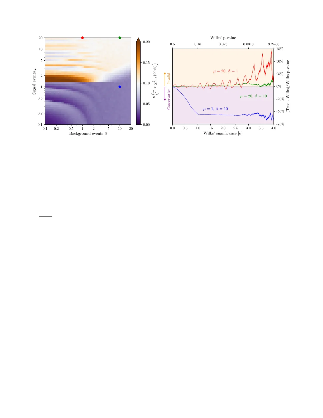
Sear ching f or ne w ph ysics with pr ofile likelihoods: Wilks and be y ond Sara Algeri 1 , Jelle Aalbers 2 , Knut Dundas Mor ˚ a 2,3 , and Jan Conrad 2,* 1 School of Statistics, Univ ersity of Minnesota, Minneapolis (MN), 55455, USA 2 Ph ysics Depar tment and Oskar Klein Centre, Stoc kholm University , Stockholm, Sw eden 3 Ph ysics Depar tment, Columbia University , New Y ork, NY 10027, USA * e-mail: conrad@fysik.su.se ABSTRA CT P ar ticle ph ysics experiments use likelihood ratio tests e xtensively to compare h ypotheses and to constr uct confidence intervals . Often, the null distribution of the likelihood ratio test statistic is appro ximated b y a χ 2 distribution, f ollowing a theorem due to Wilks. Howe v er , many circumstances rele vant to modern e xper iments can cause this theorem to f ail. In this paper , we re view how to identify these situations and construct valid inf erence. Ke y points Necessary conditions for the Likelihood Ratio T est to be approximated χ 2 include the following. • The sample size must be sufficiently large. If not, higher-order asymptotic results e xist or one can rely on Monte Carlo simulations. • The true values of the parameters must lie in the interior of the parameter space. If not, both asymptotic results and simulations must be ad- justed accordingly . • The parameters must be identifiable. If not, look- elsewhere ef fect correction methods can be of help to address this problem. • The models under comparison must be nested. If not, one can construct a comprehensive model which includes the models considered as special cases. • The models under comparison must be specified correctly . If not, adding nuisance parameters can be of help, otherwise one must rely on nonpara- metric methods. W ebsite summary: The goal of this manuscript is to identify situations in particle physics where the lik elihood ratio test statistic cannot approximated by a χ 2 distribution and propose adequate solutions. 1 Introduction Modern particle physics emplo ys elaborate statistical methods to enhance the physics reach of e xpensiv e experiments and large collaborations. The field’ s standard for reporting results is frequentist hypothesis testing. At its heart, this is a two-step recipe for distinguishing a null hypothesis H 0 (e.g. the stan- dard model) from a more general case H 1 (e.g. the standard model with a new particle): Frequentist hypothesis testing 1. Summarize the data collected by the e xperiment with a test statistic T whose absolute value is smaller under H 0 than it is under H 1 . 2. Compute a p-v alue, i.e., the probability that T is larger than its observ ed v alue when H 0 is true. H 0 is rejected if the p-value is belo w some thresh- old α (e.g. 2 . 9 × 10 − 7 , corresponding to a 5 σ significance lev el). Commonly , H 0 dif fers from H 1 for some fix ed v alues of the parameter(s) of inter est which we denote by µ , i.e., H 0 : µ = µ 0 versus H 1 : µ > µ 0 (or µ 6 = µ 0 ) . (1) The model under study may also be characterized by a set of nuisance par ameter(s) , namely θ , whose v alue is not of direct interest for the test being conducted, but it still needs to estimated under both hypotheses. F or example, in a search for a new ph ysics, µ may correspond to the rate or cross-section of signal e vents and θ could include detector ef ficiencies or uncertain background rates. T o assess the presence of the signal we test The first step of hypothesis testing requires the specification of a test statistic T . Among the wide variety of testing proce- dures av ailable in statistical literature, a popular choice is the profile (or generalized) Likelihood Ratio T est (LR T), due to its statistical power 1 , 2 and simple implementation. The LR T has been used in sev eral seminal studies in particle physics, from the discov ery of the Higgs boson 3 , 4 and measurements of the neutrino properties 5 to direct 6 – 8 and indirect 9 , 10 searches for dark matter . Gi ven a lik elihood function , L , that measures the probability of the observ ed data for a gi ven value of the parameters µ and θ , the LR T is defined as T = − 2 log L ( µ 0 , b θ 0 ) L ( b µ , b θ ) . (2) Here µ 0 is the v alue of µ specified under the null hypothesis in ( 1 ) , whereas b θ 0 is the best-fit of the nuisance parameter under H 0 , i.e., the value of θ that maximize L giv en that µ = µ 0 . Similarly , b µ and b θ are the best-fit parameters under H 1 . In the ne w physics signal search example, µ 0 = 0 (i.e., the only value of µ allowed under the null hypothesis zero); it follo ws that T is zero if b µ = 0, and it is positiv e otherwise. The second step of hypothesis testing is to quantify the evidence in f av or of H 1 by means of a p-value, i.e., the proba- bility that, when the null hypothesis is true, T is much larger than its value observ ed on the data. Finally , H 0 is excluded if the p-value if smaller than the predetermined probability of false discov ery α . An equiv alent statement on the validity of H 0 can be made by constructing a confidence interv al for µ . The latter corre- sponds to the set of possible v alues µ 0 for which the probabil- ity that T is smaller or equal than its value observ ed is 1 − α . An experiment can exclude a certain v alue µ 0 at a confidence lev el (or covera ge ) 1 − α if such value is not contained in the confidence interval. Both test of hypothesis and confidence intervals rely on the distribution of T under H 0 . A famous result from W ilks 11 states that the null distrib ution of the LR T in ( 2 ) is approxi- mately χ 2 distributed if sufficient data is acquired, pro vided some regularity conditions are met. These same results pro- vide the underpinning for the common χ 2 fitting and goodness- of-fit computations. Therefore, they are subject to the same regularity conditions, which, if incorrectly assumed, can yield to in valid claims of e xclusions or discov eries. In this paper , we present a set of necessary conditions for W ilks’ theorem to hold using language and examples familiar to particle physicists. Furthermore, when they fail, we gi ve recommendations on when extensions of W ilks’ result apply . Generally speaking, a viable alternati ve when Wilks or similar results fail to hold is to estimate the null distrib ution of T by Monte Carlo or toy simulations, i.e. simulating man y datasets under H 0 , and computing T for each. Howe ver , as discussed in Sections 3.2 and 4 , besides the computational burden, additional complications may arise and consistec y of the numerical solution is not guaranteed. 2 Wilks’ theorem and conditions W ilks’ theorem 11 can be stated as follows: Theorem (W ilks, 1938) . Under suitable r e gularity conditions, when H 0 in ( 1 ) is true, the distrib ution of T con verg es to χ 2 m . Here χ 2 m is a chi-squared random v ariable with degrees of freedom m equal to the number of parameters in µ . Instruc- tions on constructing confidence regions and tests based on W ilks’ theorem can be found elsewhere 12 ; here, we focus on − 5 − 4 − 3 − 2 − 1 0 1 2 3 4 5 E [arbitrary units] 0 . 0 0 . 5 1 . 0 1 . 5 2 . 0 2 . 5 3 . 0 Exp ected ev en ts / dE µ β γ φ 0 φ 1 E ( i ) Figure 1. An illustration of the example model used in this paper . The figure sho ws the distributions of ener gies of particles measured by an experiment. In the analysis, the aim is to constrain the mean number µ of signal ev ents from the Gaussian signal (red) centered at E = γ , on top of the polynomial background (blue) with distribution B ( E ) = φ 0 + φ 1 E + . . . and β expected number of ev ents. The model shown here is µ = 4, β = 10, γ = 0, φ 0 = 1, φ 1 = − 0 . 1 , { φ j } j ≥ 2 = 0 . The black dots show one dataset of ev ents { E ( i ) } N i = 1 that the experiment might observe under this model. the conditions needed for this theorem to apply . A formal statement of the regularity conditions required by W ilks can be found in 13 and 14 , but fi ve necessary conditions cov er most practical cases: Necessary conditions for W ilks’ theorem A S Y M P T OT I C : Suf ficient data is observed. I N T E R I O R : Only v alues of µ and θ which are far from the boundaries of their parameter space are admitted. I D E N T I FI A B L E : Dif ferent values of the parame- ters specify distinct models. N E S T E D : H 0 is a limiting case of H 1 , e.g. with some parameter fixed to a sub-range of the entire parameter space. C O R R E C T : The true model is specified either under H 0 or under H 1 . T o illustrate these conditions, we consider an experi- ment that measured N particles with ener gies E ( i ) , with i ∈ { 1 , 2 , . . . , N } , and the interest is in the mean number µ of signal ev ents on top of an expected background of β expected ev ents. The signal’ s ener gies are assumed to fol- low a Gaussian distribution with mean γ and standard devi- ation 1, while the background distribution B is polynomial, i.e. B ( E ) = k ( φ 0 + φ 1 E + φ 2 E 2 + . . . ) , with k a normalization 2/ 9 0.1 0.2 0.5 1 2 5 10 20 Bac kground ev en ts β 0.1 0.2 0.5 1 2 5 10 20 Signal ev en ts µ 0 . 00 0 . 05 0 . 10 0 . 15 0 . 20 P  T > χ 2 d =1 (90%)  0 . 0 0 . 5 1 . 0 1 . 5 2 . 0 2 . 5 3 . 0 3 . 5 4 . 0 Wilks’ significance [ σ ] -75% -50% -25% 0% 25% 50% 75% (T rue - Wilks)/Wilks p-v alue µ = 20, β = 10 µ = 1, β = 10 µ = 20, β = 1 In v alid Conserv ativ e 0.5 0.16 0.023 0.0013 3.2e-05 Wilks’ p-v alue Figure 2. Difference between true and W ilks-based p-values for the e xample experiment (see Figure 1 and eq. 3 ) with a flat background ( B ( E ) = φ 0 ), no nuisance parameters, and only allowing µ ≥ 0. Left : T rue p-v alue of T ’ s with a W ilks-based p-v alue of 0.1 ( T = χ 2 m = 1 ( 90% ) ≈ 2 . 71 ), for dif ferent true µ and β . Each square on the figure represents the model at its center , based on 10 5 toy simulations. Right : Relative error in W ilks-based p-values for dif ferent significance lev els, based on 10 7 toy simulations. Each curve corresponds to a model indicated with a dot of the same color on the left panel. constant, e.g., Figure 1 . For an (extended) unbinned analysis, the likelihood func- tion is: L = 1 µ + β Poisson ( N | µ + β ) N ∏ i = 1 h β B ( E ( i ) ) + µ Gauss ( E ( i ) − γ ) i . (3) Here, Poisson ( N | µ + β ) is the probability mass function of the Poisson distribution with mean µ + β , and Gauss the prob- ability density function of a standard normal. For a disco very test, H 0 typically specifies as µ = 0 and H 1 is either µ > 0 (when only positiv e signals are allowed) or µ 6 = 0 (as in some neutrino oscillation experiments 5 ). Finally , we consider as nuisance parameters collected in θ the set ( β , γ , φ 0 , φ 1 , . . . ) . W e can no w describe each of the conditions necessary for W ilks to hold. • T echnically , A S Y M P T OT I C I T Y requires N → ∞ . W e will consider practical requirements in the next section. • The true values of the both the parameters of interest and the nuisance parameters are in the I N T E R I O R of their respectiv e parameter space. For instance, under H 0 , it would fail if only positiv e signals were allowed ( µ ≥ 0 ). • Each parameter is I D E N T I FI A B L E –i.e., different values of the parameters specify different models. In our example, this holds if the signal location γ is known. Whereas, the model is not identifiable when γ is unknown and the signal is absent ( µ = 0). • In our example, H 0 : µ = 0 is a limiting case of H 1 : µ > 0 (or H 1 : µ 6 = 0 ) hence we say that the models are N E S T E D . This would not be the case, for instance, when testing H 0 : µ = 0 versus H 1 : µ = 1. • The experiment’ s model is C O R R E C T . It would fail e.g. if the experiment has an additional unmodeled background component. If the abov e-mentioned conditions hold, under H 0 , the dis- tribution of T follows a χ 2 m . In our e xample, m = 1 since our hypotheses differ only in a single parameter µ , i.e., the expected number of signal e vents. 3 Failures of Wilks in practice 3.1 Insufficient data Physics searches, e.g. for dark matter or neutrinoless double- beta decay , often look for rare signals on top of backgrounds they attempt to minimize. If the signal is weak or the back- ground is low , e.g. because the experiment ran only for a short time, there may be insuf ficient data for an A S Y M P T OT I C approximation such as W ilks to be valid or to be able to dis- criminate the signal from the background distribution. The left panel of Figure 2 sho ws the dif ference between true and W ilks’-based p-v alues for our example experiment, for a flat background B = φ 0 and while increasing the num- ber of signal ev ents µ 0 expected under H 0 . The case of low background and moderate signal (red in Figure 2 ), clearly illustrates the ef fect of a non- A S Y M P TO T I C test. The true significance for a certain χ 2 -threshold undulates around the desired significance, due to the discrete number of observ ed ev ents and ultimately the Poisson term in equation 3 . Only if both β and µ 0 are large (green in Figure 2 ) W ilks’ approxima- tion becomes accurate. 3/ 9 γ T ( γ ) c 0 Figure 3. Upcrossings (red crosses) of a threshold c 0 by { T ( γ ) } (blue line). Mathematically , W ilks’ requirement of asymptoticity en- sures that the best-fit parameters, in our example b µ and b θ , known as maximum-lik elihood estimates (MLEs), are nor- mally distrib uted with mean equal to their true v alue. Con- sequently , the χ 2 approximation deriv ed by W ilks holds to order O ( N − 1 ) . Higher-order lik elihood theory giv es alterna- tiv e test statistics whose distrib utions con verge to O ( N − 3 / 2 ) , as re viewed comprehensively in [ 15 , Sec 2.2]. Howe ver , these statistics are often dif ficult to implement 16 , 17 ; therefore, using simulations to estimate the null distribution of T is often more practical. 3.2 Parameter s with bounds In many cases, parameters of statistical models may be con- strained ov er a closed interval. Examples include particle masses or e vent rates that can only take positiv e values. In our example, this corresponds to the situation where µ ∈ [ 0 , ∞ ) . Therefore, µ = 0 is a boundary point and thus, under H 0 , µ is not in the I N T E R I O R of its parameter space. In this situa- tion, W ilks theorem ultimately fails because the distrib ution of MLE is normal 50% times and it takes value zero on the remaining 50%. When one or more of the parameters of interest are tested on the boundary of their parameter space, the limiting distri- bution of T under H 0 is not χ 2 , but it may still enjoy a simple approximation. In our positive-signal example, the limiting T distribution at the boundary µ = 0 is 1 2 χ 2 m = 1 + 1 2 δ ( 0 ) , with δ ( 0 ) being the delta-Dirac function centered at zero. This scenario was first studied by Chernoff 18 and later extended by others (e.g., 19 ) to more general situations. Specifically , Self and Liang 19 show that, if the true v alues of the nuisance parameters also lie on boundaries, the distribution of T under H 0 becomes more complex. In this setting, the limiting distri- bution may dif fer over dif ferent re gions of the parameter space and its asymptotic approximation may become particularly challenging (e.g., [ 19 , Case 7]). Unfortunately , when the true values of the nuisance param- eters lie on the boundaries of the parameter space, simulations based on the MLE can lead to inconsistent results 20 . Howe ver , estimators designed can be used instead of the MLE to av oid this problem 20 – 22 . As a more specific example of a boundary , when the true value of µ mov es close to the boundary in µ = 0 in figure 2 , the MLE of µ ends up at the border more often, and the test statistic distribution morphs from W ilks’ result to Chernoff ’ s 1 2 χ 2 m = 1 + 1 2 δ ( 0 ) at µ = 0 . T oy Monte Carlo simulations may be necessary to determine if the signal is lar ge/small enough to be at either extreme. This will also depend on the signif- icance level desired, as shown for the model shown in blue in figure 2 (with β = 10 and µ 0 = 1 ), where Chernoff ’ s theo- rem approximately holds for significances corresponding to p = 0 . 1 , with 0 . 05 of tests exceeding χ 2 1 ( 90% ) . This extends to the entire lo wer right re gion, with µ . 1 and β & 5 for confidence lev els of 0 . 05. 3.3 Non-identifiability and look-elsewhere effects Sev eral theories of new physics often feature unknown pa- rameters, such as the mass of a new particle. F or the model in ( 3 ) , this corresponds to the situation where the location of the signal, γ , is unknown. If the signal is absent ( H 0 : µ = 0 ), γ is a non-identifiable parameter: one that does not actually change the predictions of the experiment. Non-identifiability of a nuisance parameter implies that the limit of the respective MLE does not exist. Consequently , consistency and normality of the MLE are not guaranteed and W ilks’ theorem fails to hold. Searches for ne w particles typically consider any v alue of γ to which the experiment is sensiti ve. If the experiment wishes to report a separate confidence for each location, as may be the case with upper limits, a series of test statistics { T ( γ ) } , one for each v alue of γ fixed, can be employed. The most significant result (i.e. the lo west p-v alue) can then be identified as an excess if it e xceeds the field-specific thresholds. Howe ver , when sev eral tests are conducted simultaneously the, look-elsewher e effect (LEE) applies, i.e., the inference must be adjusted to preserve the desired (global) significance lev el α , i.e., the probability of having at least one false detec- tion among all the tests considered. Unfortunately , classical multiple h ypothesis testing procedures such as Sidak’ s or Bon- ferroni’ s corrections (see [ 23 , Ch. 3]) either assume the tests are independent one another or are e xcessiv ely conservati ve. Unfortunately , the assumption of independence among the tests typically does not apply when γ corresponds to the sig- nal location as models testing for signals in nearby locations can only be weakly distinguished and thus the resulting tests would be highly correlated. Gross and V itells 24 introduced a nov el approach to reduce the amount of Monte Carlo samples needed when nuisance parameters are not I D E N T I FI A B L E under the null hypothe- sis. Their method aims to approximate the null distribution of max γ { T ( γ ) } to deriv e a (global) p-v alue for the test H 0 : µ = 0 versus H 1 : µ > 0 . When µ can take both positi ve and ne gativ e values, and assuming that the process { T ( γ ) } is distrib uted as a χ 2 random process, the probability that max γ { T ( γ ) } ex- ceeds a high threshold c can be approximated by the expected number of times { T ( γ ) } upcrosses a lo wer threshold c 0 (see 4/ 9 0 1 2 3 4 5 6 7 t P ( T ≥ t ) (log 10 −scale) β = 100 χ m = 1 2 T for φ 0 + φ 1 x T for φ 0 + φ 1 x + φ 2 x 2 T for φ 0 + φ 1 x + φ 2 x 2 + φ 3 x 3 T for φ 0 + φ 1 x + φ 2 x 2 + φ 3 x 3 + φ 4 x 4 0.01 0.1 0.5 0 1 2 3 4 5 6 7 t P ( T ≥ t ) (log 10 −scale) β = 1000 χ m = 1 2 T for φ 0 + φ 1 x T for φ 0 + φ 1 x + φ 2 x 2 T for φ 0 + φ 1 x + φ 2 x 2 + φ 3 x 3 T for φ 0 + φ 1 x + φ 2 x 2 + φ 3 x 3 + φ 4 x 4 0.01 0.1 0.5 0 1 2 3 4 5 6 7 t P ( T ≥ t ) (log 10 −scale) β = 10000 χ m = 1 2 T for φ 0 + φ 1 x T for φ 0 + φ 1 x + φ 2 x 2 T for φ 0 + φ 1 x + φ 2 x 2 + φ 3 x 3 T for φ 0 + φ 1 x + φ 2 x 2 + φ 3 x 3 + φ 4 x 4 0.01 0.1 0.5 Figure 4. P-values approximations for ( 1 ) with µ 0 = 0 when increasing the number of nuisance parameters and the expected number of ev ents. The bias-variance trade-of f plays a prominent role in approaching the χ 2 m = 1 distribution (black solid line). When β = 100 (left panel) the sample size is not lar ge enough to achieve a reliable χ 2 m = 1 approximation for none of the models considered. When increasing the expected number of e vents to β = 1000 (central panel) both the 3 rd and 4 t h degree polynomials (green dashed line and blue solid line, respectiv ely) approach the χ 2 approximation. In this case, despite the 4 t h degree polynomial has zero bias, it suf fers from higher variance than the cubic polynomial and thus the y both lead to a reasonable χ 2 approximation. Howe ver , when β = 10000 (right panel) only the 4 t h polynomial leads to a reliable χ 2 m = 1 approximation. Figure 3 ) and denoted by E [ N c 0 | H 0 ] . Specifically , as c → ∞ P ( max γ { T ( γ ) } > c | H 0 ) ≈ P ( χ 2 m = 1 > c ) + E [ N c 0 | H 0 ] e − ( c − c 0 ) 2 (4) Despite E [ N c 0 | H 0 ] has to be estimated by simulation, it re- quires less Monte Carlo toys than those needed to estimate accurately the p-value of the high threshold c directly . Fur - thermore, although the approximation in equation ( 4 ) is valid as c → ∞ , the right hand side bounds the left hand side from abov e for small values of c . Thus, the approximation yields to inference that might be overly conserv ativ e, but will not ov erstate an excess. 3.4 Non-nestedness Many problems in physics in volve the comparison of models which are not N E S T E D , i.e., one cannot be specified as a limiting case of the other . Examples include when testing the sign of an ef fect with known rate, or more commonly , when deciding between two incompatible functional forms such as (broken) po wer-la ws and an exponential energy cutof f 25 . The issue arising in this setting is that, despite the MLEs of the parameters of the two models are Gaussian, they do not share the same parameter space and thus T is not guaranteed to be χ 2 distributed. A simple solution to the non-nested problem is to enlarge the model to one that co vers both models under comparison as special cases. For example, suppose the goal is to decide be- tween tw o models f and g (e.g., two distributions of ener gies), each characterized by its own set of unknown parameters. W e consider the comprehensi ve model h = η f + ( 1 − η ) g . Here 0 ≤ η ≤ 1 is a ne w parameter with no physical meaning b ut it is of crucial importance to perform inference. Specifically , two tests are constructed, i.e., H 0 : η = 0 versus H 1 : η > 0 (5) H 0 : η = 1 versus H 1 : η < 1 . (6) and f is selected if ( 5 ) rejects H 0 but ( 6 ) does not. Whereas, g is selected if H 0 is rejected in ( 6 ) but it is not in ( 5 ) . In all the other cases the test is said to be inconclusiv e. In this construction η is not in the I N T E R I O R of parameter space. Moreover , the parameters in f and g are not I D E N T I FI - A B L E under H 0 in ( 5 ) or ( 6 ) . Howe ver , recent work 26 – 29 has shown that the result of Gross and V itells can be extended to cov er this case; the χ 2 m = 1 term in equation ( 4 ) acquires a factor 1 / 2 because the parameter µ is tested on a boundary . Exten- sions of 24 and 26 to multiple dimensions are presented in 28 – 30 , whereas 28 , 31 discuss the precise conditions that guarantee the validity of the resulting inference. It is important to point out that if f and g do not contain an y unknown parameters, the problem is substantially simplified since, because of the Central Limit Theorem, the ratio of the likelihoods follo ws a Normal distribution 32 . 3.5 Uncer tain models and n uisance parameters Experiments often have uncertainties on the nuisance parame- ters, such as detection ef ficiencies or background rates. As a result, the models under either H 0 or H 1 may not be correctly 5/ 9 Figure 5. Distribution of T for a counting experiment with true signal expectation of µ = 2 ev ents, a known background of β = 0 . 5 events, and a detection ef ficiency ε = 0 . 9. The efficienc y is either considered known (gray), or as a nuisance parameter . In the latter case, a constraint term Gaussian (( ε − ε measured ) / σ ε ) corresponding to the distribution of a subsidiary measurement ε measured is added to the likelihood (eq. 3 ). The T distribution for σ = 0 . 02 (blue) and σ = 0 . 3 (orange) is plotted. specified and thus the last of our necessary conditions fails to hold. A common remedy is to introduce additional nuisance pa- rameters in order to increase the fle xibility of the model and reduce its bias , i.e., the discrepancy between the true underly- ing model and the model considered. On the other end, adding more parameters may substantially increase the variance of the MLEs. Therefore, when specifying the background and/or signal models one must account for the trade-of f between bias and variance. T o illustrate this phenomenon, we consider once again our example e xperiment. Suppose that the true (unknown) back- ground is distributed as a fourth-order polynomial which we attempt to model with increasingly higher order polynomials. W e aim to test H 0 : µ = 0 versus H 0 : µ 6 = 0 . In order to av oid boundary problems we allow µ to be ne gativ e. As Figure 4 sho ws, when the e xperiment assumes a lin- ear background (red chained lines), the null distribution is substantially different from the one obtained assuming the true model (blue solid lines). Whereas, as expected, the fit gets closer and closer to the truth when the polynomial or- der increases as this leads to a reduction of the bias. More interesting, howe ver , is the effect played by the v ariance. Specifically , when the sample size decreases, the quadratic (orange chained lines) and cubic (green dashed lines) fits get closer to the one obtained with a fourth degree polynomial. This is because, the v ariance increases when the sample size decreases but it is reduced for models with a smaller number of parameters. This is further emphasizes by the fact that for small or only moderately large sample sizes, e.g., β = 100 or β = 1000 both the fourth and the third degree polynomial provide a similar fit. Howe ver , when the expected number of ev ents increases substantially ( β = 1000) the v ariance is dra- matically reduced while the bias of the cubic fit is preserved. Remarkably , introducing nuisance parameters can some- times help the achiev e a χ 2 approximation in non-asymptotic conditions, as illustrated in Figure 5 . Here, we consider an experiment with indistinguishable signal and background (a ‘counting experiment’) and lo w expected counts. If the detec- tion ef ficiency ε is kno wn, T ’ s distribution is that of a (scaled) low-count Poisson, which de viates strongly from the asymp- totic χ 2 -distribution. Howe ver , if ε is a nuisance parameter with a relativ ely broad constraint, the test statistic distrib ution is smeared out, and the asymptotic approximation performs better . When the model imposes a functional form which is sub- stantially different from the true model, e.g. imposing a double exponential structure to fit data generated from a po wer law , additional nuisance parameters are unlikely to solve the prob- lem. In this case, one can resort to nonparameteric methods 33 , or other conserv ativ e procedures 34 , 35 to correct mismodelling. 4 Recommendations When applying Wilks theorem, or more generally , when using the χ 2 formalism to calculate p-values or confidence intervals, one has to be a ware of the regularity conditions that make this possible. Here we presented fi ve conditions necessary for W ilks to hold and which should be suf ficiently practical to serve as rules of thumbs on the applicability of the χ 2 approx- imation for the LR T . Specifically , the conditions I N T E R I O R , I D E N T I FI A B L E , N E S T E D and C O R R E C T refer to specific prop- erties of the model under study . Thus, by studying the model in depth, it should be possible to understand whether they are fulfilled. The condition A S Y M P TO T I C refer to the size of the data av ailable. Therefore, its v alidity is typically dictated by the specifics of the experiment being conducted. T able 1 outlines the solutions proposed in this paper to address the failure of each of the necessary conditions consid- ered. Specifically , our recommendations can be summarized as follows. • If the data is not suf ficiently lar ge to guaranteed the v a- lidity of classical A S Y M P T OT I C results, one can refer to approximations based on higher-order asymptotic lik eli- hood theory or Monte Carlo simulations. Ho we ver , the reader must keep in mind that the former suf fers from substantial mathematical complexity while the latter re- quires the av ailability of sufficient computational po wer . • If the true v alues of the parameters are not in the I N - T E R I O R of their parameter space, one can implement boundary corrections for the p-values on the basis of the results of Chernoff 18 , Self and Liang 19 and related works. Con versely , when aiming to address the prob- lem by means of simulations, classical estimators of the 6/ 9 A S Y M P T OT I C I N T E R I O R I D E N T I F I A B L E N E S T E D C O R R E C T W ilks’ theorem 3 3 3 3 3 Higher order asymptotics 7 3 3 3 3 Boundary corrections 3 7 3 3 3 LEE corrections 3 : 7 3 3 T ests for non-nested models 3 3 3 7 3 Monte Carlo methods 7 : 7 7 3 Use of nuisance parameters : : : : : Nonparametric methods 7 7 7 7 7 T able 1. Inference under non-re gular settings. Green check marks indicate that the condition in the respective column must hold for the method on the left to be reliable. Orange plus marks indicate that extensions exists to co ver situations where the respectiv e condition does not hold (see text). Red cross marks indicate that the method on the left can be applied e ven if the condition in the respectiv e column does not hold. nuisance parameters must be replaced by more efficient estimators 20 – 22 to guarantee consistency of the solution. • If nuisance parameters are not I D E N T I FI A B L E and a fully simulated solution is excessi vely e xpensiv e, corrections for the LEE such as Gross and V itells 24 and respectiv e extensions allow to perform inference while reducing drastically the number of simulations required. • If the models under comparison are non- N E S T E D , a sim- ple solution is to specify a model which include the models under study as special cases 33 . • If the likelihood specified is not C O R R E C T , one may attempt to recover the structure of the true underlying model by adding nuisance parameters and apply an y of the abov e mentioned inferential methods. As any other modelling strategy , ho wev er , the bias-variance trade-of f must be taken into account. Finally , if none of the assumptions above holds, or the correct models cannot be recovered by simply adding nuisance parameters, the only solution is to refer to nonparameteric methods (e.g., 33 ) for both statistical modelling and inference. References 1. Neyman, J. & Pearson, E. S. Ix. on the problem of the most efficient tests of statistical hypotheses. Philos. T rans- actions Royal Soc. London. Ser. A, Containing P ap. a Math. or Phys. Character 231 , 289–337 (1933). 2. Karlin, S. & Rubin, H. The theory of decision pro- cedures for distributions with monotone likelihood ra- tio. Ann. Math. Stat. 27 , 272–299, DOI: 10.1214/aoms/ 1177728259 (1956). 3. Aad, G. et al. Observation of a ne w particle in the search for the Standard Model Higgs boson with the A TLAS detector at the LHC. Phys. Lett. B716 , 1–29, DOI: 10. 1016/j.physletb .2012.08.020 (2012). 1207.7214 . 4. Chatrchyan, S. et al. Observ ation of a New Boson at a Mass of 125 GeV with the CMS Experiment at the LHC. Phys. Lett. B716 , 30–61, DOI: 10.1016/j.physletb .2012. 08.021 (2012). 1207.7235 . 5. An, F . P . et al. Observation of electron-antineutrino disap- pearance at Daya Bay. Phys. Re v . Lett. 108 , 171803, DOI: 10.1103/PhysRe vLett.108.171803 (2012). 1203.1669 . 6. Aprile, E. et al. Dark Matter Search Results from a One T on-Y ear Exposure of XENON1T. Phys. Rev. Lett. 121 , 111302, DOI: 10.1103/PhysRe vLett.121.111302 (2018). 7. PandaX-II Collaboration et al. Dark Matter Results from 54-T on-Day Exposure of PandaX-II Experiment. Phys. Rev. Lett. 119 , 181302, DOI: 10.1103/PhysRe vLett.119. 181302 (2017). 8. Akerib, D. S. et al. Results from a search for dark matter in the complete LUX exposure. Phys. Re v. Lett. 118 , DOI: 10.1103/PhysRe vLett.118.021303 (2017). 1608.07648 . 9. Abdallah, H. et al. Search for γ -Ray Line Signals from Dark Matter Annihilations in the Inner Galactic Halo from 10 Y ears of Observations with H.E.S.S. Phys. Rev . Lett. 120 , 201101, DOI: 10.1103/PhysRe vLett.120. 201101 (2018). 1805.05741 . 10. Ackermann, M. et al. Updated search for spectral lines from Galactic dark matter interactions with pass 8 data from the Fermi Large Area T elescope. Phys. 7/ 9 Rev . D91 , 122002, DOI: 10.1103/PhysRe vD.91.122002 (2015). 1506.00013 . 11. W ilks, S. The large-sample distribution of the likelihood ratio for testing composite hypotheses. The Annals Math. Stat. 9 , 60–62 (1938). Definition of Wilks’ theor em . 12. Cow an, G., Cranmer , K., Gross, E. & V itells, O. Asymptotic formulae for likelihood-based tests of new physics. The Eur. Phys. J. C 71 , 1554, DOI: 10.1140/epjc/s10052- 011- 1554- 0, 10.1140/epjc/ s10052013- 2501- z (2011). [Erratum: Eur . Phys. J.C73,2501(2013)] Collects likelihood ratio test statistics used for discov- ery significance and confidence intervals in physics, and descibes their asymptotic properties. 13. Cox, D. R. & Hinkley , D. V . Theor etical statistics (Chap- man and Hall/CRC, 1979). P .281. 14. Protassov , R., V an Dyk, D. A., Connors, A., Kashyap, V . L. & Siemigino wska, A. Statistics, handle with care: detecting multiple model components with the likelihood ratio test. The Astr ophys. J. 571 , 545 (2002). 15. Brazzale, A. R. & V alentina, M. Likelihood asymptotics in nonregular settings. a revie w with emphasis on the likelihood ratio. W orking P aper Series 4 , Department of Statistical Sciences, Univ ersity of Pado va (2018). 16. Sev erini, T . A. An empirical adjustment to the likelihood ratio statistic. Biometrika 86 , 235–247 (1999). 17. He, H., Sev erini, T . A. et al. Higher-order asymptotic normality of approximations to the modified signed like- lihood ratio statistic for regular models. The Annals Stat. 35 , 2054–2074 (2007). 18. Chernoff, H. On the distribution of the likelihood ra- tio. Ann. Math. Stat. 25 , 573–578, DOI: 10.1214/aoms/ 1177728725 (1954). Examines the distribution of the Log-Likelihood ra- tio when the true value lies at the boundary separat- ing the null and alternativ e hypothesis. 19. Self, S. G. & Liang, K.-Y . Asymptotic properties of maximum likelihood estimators and likelihood ratio tests under nonstandard conditions. J. Am. Stat. Assoc. 82 , 605–610 (1987). An extension of Chernoffs r esult on likelihood ratio tests where one or more parameters lie on bound- aries. 20. Andrews, D. W . Inconsistency of the bootstrap when a parameter is on the boundary of the parameter space. Econometrica 68 , 399–405 (2000). 21. Geyer , C. J. Likelihood ratio tests and inequality con- traints. T ech. Rep., University of Minnesota (1995). 22. Cav aliere, G., Nielsen, H. B., Pedersen, R. S. & Rahbek, A. Bootstrap inference on the boundary of the parameter space with application to conditional v olatility models. A vailable at SSRN 3282935 (2018). 23. Efron, B. Lar ge-scale infer ence: empirical Bayes meth- ods for estimation, testing, and pr ediction , vol. 1 (Cam- bridge Univ ersity Press, 2012). 24. Gross, E. & V itells, O. T rial factors for the look elsewhere effect in high energy physics. The Eur. Phys. J. C 70 , 525–530 (2010). 25. Aharonian, F . et al. Spectrum and variability of the Galactic center VHE γ -ray source HESS J1745-290. As- tr on. Astr ophys. 503 , 817–825, DOI: 10.1051/0004- 6361/ 200811569 (2009). 0906.1247 . 26. Algeri, S., Conrad, J. & van Dyk, D. A. A method for comparing non-nested models with application to astro- physical searches for ne w physics. Mon. Not. Roy . As- tr on. Soc. 458 , L84–L88, DOI: 10.1093/mnrasl/slw025 (2016). Extends the Gr oss and V itells method to the pr oblem of non-nested hypothesis testing , 1509.01010 . 27. Algeri, S. & van Dyk, D. A. T esting one hypothesis mul- tiple times. Stat. Sinica (to appear). (2019). 28. Algeri, S. & van Dyk, D. A. T esting one hypothesis mul- tiple times: The multidimensional case. arXiv pr eprint arXiv:1803.03858 (2018). 29. Algeri, S. et al. Statistical challenges in the search for dark matter . arXiv pr eprint arXiv:1807.09273 (2018). 30. V itells, O. & Gross, E. Estimating the significance of a signal in a multi-dimensional search. Astr opart. Phys. 35 , 230–234 (2011). Efficient method for computing the look-elsewher e ef- fect with toy-Monte Carlos . 31. Davies, R. B. Hypothesis testing when a nuisance param- eter is present only under the alternati ve. Biometrika 74 , 33–43 (1987). 32. Cox, D. R. T ests of separate families of hypotheses. In Pr oceedings of the fourth Berkele y symposium on mathe- matical statistics and pr obability , v ol. 1, 23 (1961). 33. Algeri, S. Detecting new signals under background mis- modelling. arXiv preprint arXiv:1906.06615 (2019). 34. Priel, N., Rauch, L., Landsman, H., Manfredini, A. & Budnik, R. A model independent safeguard for un- binned Likelihood. J. Cosmol. Astr opart. Phys. 2017 , 013–013, DOI: 10.1088/1475- 7516/2017/05/013 (2017). 1610.02643 . 35. Y ellin, S. Finding an Upper Limit in the Presence of Unknown Background. Phys. Rev. D 66 , DOI: 10.1103/ PhysRe vD.66.032005 (2002). physics/0203002 . 8/ 9 Ackno wledgements J.C., J.A. and K.D.M. gratefully acknowledge support from the Knut and Alice W allenber g Foundation, and the Swedish Research Council. A uthor contributions The authors contributed equally to all aspects of the article. Competing interests The authors declare no competing interests. 9/ 9