Lossless Image and Intra-frame Compression with Integer-to-Integer DST

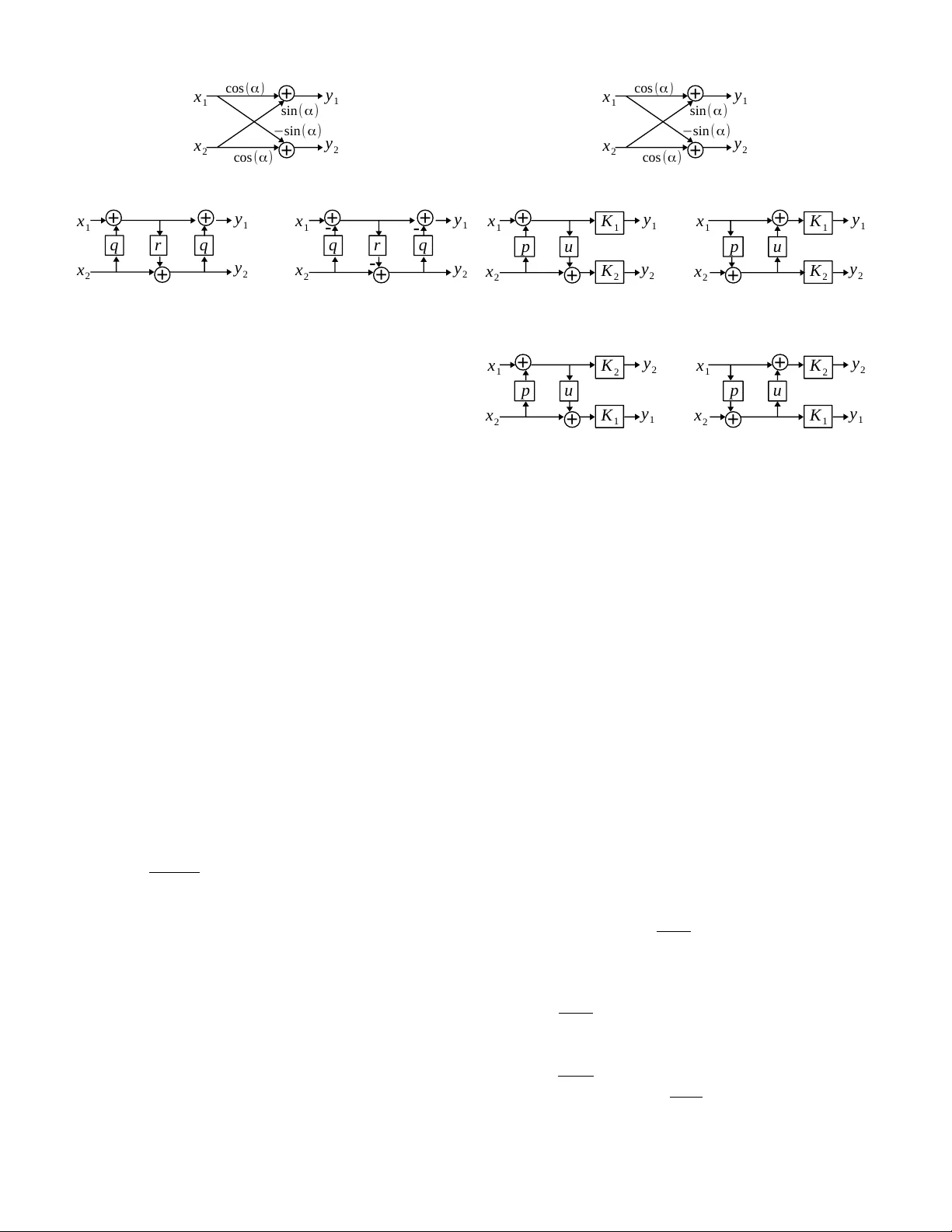
1 Lossless Image and Intra-frame Compression with Inte ger -to-Inte ger DST Fatih Kamisli, Member , IEEE Abstract —V ideo coding standards are primarily designed f or efﬁcient lossy compression, b ut it is also desirable to support efﬁcient lossless compression within video coding standards using small modiﬁcations to the lossy coding architecture. A simple approach is to skip transform and quantization, and simply entropy code the prediction residual. Howev er , this approach is inefﬁcient at compression. A more efﬁcient and popular approach is to skip transf orm and quantization b ut also process the r esidual block with DPCM, along the horizontal or vertical direction, prior to entropy coding. This paper explores an alternati ve approach based on processing the residual block with integer-to- integer (i2i) transforms. I2i transforms can map integer pixels to integer transform coefﬁcients without incr easing the dynamic range and can be used for lossless compression. W e focus on lossless intra coding and develop novel i2i approximations of the odd type-3 DST (ODST -3). Experimental r esults with the HEVC refer ence software show that the developed i2i approximations of the ODST -3 improve lossless intra-frame compression efﬁciency with respect to HEVC version 2, which uses the popular DPCM method, by an av erage 2.7% without a signiﬁcant effect on computational complexity . Index T erms —Image coding, V ideo Coding, Discrete cosine transforms, Lossless coding, HEVC I . I N T RO D U C T I O N V ideo coding standards are primarily designed for efﬁcient lossy compression, but it is also desirable to support efﬁcient lossless compression within video coding standards. Howe ver , to av oid increase in the system complexity , lossless compres- sion is typically supported using small modiﬁcations to the lossy coding architecture. Lossy compression in modern video coding standards, such as HEVC [1] or H.264 [2], is achieved with a block-based approach. First, a block of pixels are predicted using pixels either from a previously coded frame (inter prediction) or from previously coded regions of the current frame (intra prediction). The prediction is in many cases not sufﬁciently accurate and in the next step, the block of prediction error pixels (residual) are computed and then transformed to reduce remaining spatial redundancy . Finally , the transform coefﬁ- cients are quantized and entropy coded together with other relev ant side information such as prediction modes. T o support also lossless compression within the block-based lossy coding architecture summarized abov e, the simplest approach is to just skip the transform and quantization steps, and directly entropy code the prediction residual block. This approach is indeed used in HEVC version 1 [1]. While this is a simple and low-comple xity approach, it is well known that prediction residuals are not sufﬁciently decorrelated in F . Kamisli is with the Department of Electrical and Electronics Engineering at the Middle East T echnical Univ ersity , Ankara, T urkey . many re gions of video sequences and directly entropy coding a prediction residual block is inefﬁcient at compression. Hence, a large number of approaches hav e been proposed to develop more efﬁcient lossless compression methods for video coding. A more ef ﬁcient and popular approach is to skip transform and quantization but process the residual block with differen- tial pulse code modulation (DPCM) prior to entropy coding [3], [4]. While there are many v ariations of this approach [3], [4], [5], [6], video coding standards HEVC and H.264 include the simple horizontal and vertical DPCM due to their low complexity and reasonable compression performance. This paper explores an alternati ve approach for lossless compression within video coding standards. Instead of DPCM, integer -to-integer (i2i) transforms are used to process the residual block. I2i transforms can map inputs that are on a uniform discrete lattice to outputs on the same lattice and are in vertible [7]. In other words, i2i transforms can map integer pixels to integer transform coefﬁcients. Note ho wev er that unlike the integer transforms used in HEVC for lossy coding [8], i2i transforms do not increase the dynamic range at the output and can therefore be easily employed in lossless coding. While there are many papers that employ i2i approximations of the discrete cosine transform (DCT) in lossless image compression [9], we could not come across a work which explores i2i transforms for lossless compression of prediction residuals in video coding, or particularly in H.264 or HEVC. This paper focuses on lossless compression for intra coding. For lossless inter coding, some of our preliminary results are provided in [10]. In lossy intra coding, it is kno wn that a hybrid separable 2D transform based on the odd type-3 discrete sine transform (ODST -3) and the DCT [11], [12] or simply a 2D ODST -3 [1] provides improv ed compression performance ov er the traditional 2D DCT at transform coding block-based spatial prediction residuals. While the literature includes great previous research on i2i DCTs [9], [13], [14], we could not ﬁnd any i2i approximations of the ODST -3. Therefore in this paper , we ﬁrst explore the design of i2i approximations of the ODST -3 and then provide lossless intra-frame compression results with the dev eloped i2i approximations of the ODST -3. Our experimental results performed using the HEVC reference software indicate that using the de veloped i2i approximations of ODST -3, the lossless intra-frame compression of HEVC version 2, which uses the popular DPCM method along the horizontal or vertical direction, can be improved by an average 2 . 7% without signiﬁcant complexity increase. The remainder of the paper is organized as follows. In Section II, a brief overvie w of related previous research on lossless video compression is provided. Section III discusses i2i transforms and their design based on plane rotations and the 2 lifting scheme. Section IV presents a framew ork for designing computationally efﬁcient i2i approximations of the ODST -3. Section V presents experimental results with the designed i2i approximations of the ODST -3 within HEVC and compares them with those of HEVC version 1 and 2. Finally , Section VI concludes the paper . Note that some preliminary results of this work were presented in [10], [15]. I I . P R E V I O U S R E S E A R C H O N L O S S L E S S V I D E O C O M P R E S S I O N One of the simplest methods to support lossless compression within video codecs primarily designed for lossy coding is to just skip the transform and quantization steps, and directly entropy code the prediction residual block. This approach is indeed used in HEVC version 1 [1]. While this is a low- complexity approach, it is inefﬁcient at compression since prediction residuals are typically not well decorrelated. Hence, a large number of approaches hav e been proposed to develop more efﬁcient lossless compression methods for video coding. These approaches can be categorized into three groups, which we brieﬂy review as follows. A. Methods based on residual DPCM The ﬁrst group of methods are based on processing the residual blocks, obtained from the block-based spatial or temporal prediction of the lossy coding architecture, with differential pulse code modulation (DPCM) prior to entropy coding and are typically called residual DPCM (RDPCM) methods. There are many v ariations of RDPCM methods in the literature for both lossless intra and inter coding [3], [4], [5], [6]. RDPCM methods process the prediction residual block with some speciﬁc pix el-by-pixel prediction method, which is typically the distinguishing feature among the many RDPCM methods. One of the earliest RDPCM methods was proposed in [3] for lossless intra coding in H.264. Here, after the block- based spatial prediction is performed, a simple pix el-by- pixel differencing operation is applied on the residual pixels in only horizontal and vertical intra prediction modes. In the horizontal intra mode, from each residual pixel, its left neighbor is subtracted and the result is the RDPCM pixel of the block. Similar differencing is performed along the vertical direction in the vertical intra mode. Note that the residuals of other angular intra modes are not processed in [3] because directional pixel-by-pixel prediction with different interpolation for each angular prediction mode is required to account for the directional correlation of the residuals and the additional improvement in compression does not justify the complexity increase. The same RDPCM method as in [3] is now included in HEVC version 2 [16], [17] for intra and inter coding. In inter coding, RDPCM is applied either along the horizontal or vertical direction or not at all, and a ﬂag is coded in each transform unit (TU) to indicate if it is applied, and if so, another ﬂag is coded to indicate the direction. In intra coding, RDPCM is applied only when intra prediction mode is either horizontal or vertical and no ﬂag is coded since the RDPCM direction is inferred from the intra prediction mode. B. Methods based on pixel-by-pixel spatial prediction The second group of methods can be used only in lossless intra coding and are based on replacing the block-based spatial prediction method with a pix el-by-pixel spatial prediction method. Since the transform is skipped in lossless coding, a pixel-by-pix el spatial prediction approach can be used instead of block-based prediction for more efﬁcient prediction. The literature contains many lossless intra coding methods based on the pixel-by-pix el prediction approach [18], [19], [20]. The so-called Sample-based Angular Prediction (SAP) method is a well-known such method [18]. In the application of the SAP method to HEVC [18], only the angular intra modes are modiﬁed and the DC and planar intra modes remain unmodiﬁed. In these modiﬁed angular intra modes, the same angular projection directions and linear interpolation equations of HEVC’ s intra prediction are used, but the used reference samples are modiﬁed. Instead of the the block neighbor pixels, the immediate neighbor pixels are used as reference pix els for prediction, resulting in a pixel-by-pixel prediction version of HEVC’ s block-based intra prediction. Instead of using the HEVC intra prediction equations for pixel-by-pix el spatial prediction, a more general pixel-by- pixel spatial prediction method based on using 3 neighboring pixels in each intra mode of HEVC is dev eloped in [21], and the results report one of the best lossless intra coding performances within HEVC. While the lossless intra coding methods based on pixel-by- pixel spatial prediction can provide competitiv e compression performance, their distinguishing feature can also be a draw- back. Their pixel-based nature is not congruent with the block- based architecture of video coding standards and introduces undesired pixel-based dependencies in the prediction architec- ture that can reduce throughput in the processing pipeline of video encoders and decoders [18], [21]. C. Methods based on modiﬁed entr opy coding The third group of methods considers entropy coding. In lossy coding, transform coefﬁcients of prediction residuals are entropy coded, while in lossless coding, the prediction residuals are entropy coded. Considering the difference of the statistics of quantized transform coef ﬁcients and prediction residuals, se veral modiﬁcations in entropy coding were pro- posed for lossless coding [22], [23], [24]. The HEVC v ersion 2 includes reversing the scan order of coefﬁcients, using a dedicated context model for the signiﬁcance map and other tools [16], [25]. I I I . I N T E G E R - T O - I N T E G E R ( I 2 I ) T R A N S F O R MS Integer -to-integer (i2i) transforms map integer inputs to integer outputs and are inv ertible [7]. Note that unlike the integer transforms in HEVC [8], which also map integer residual pixels to integer transform coefﬁcients by implement- ing the transform operations with ﬁxed-point arithmetic, i2i transforms considered here do not increase the dynamic range at the output. Therefore they can be easily used in lossless compression. 3 + c os ( α ) + x 1 x 2 y 1 y 2 c os ( α ) s i n ( α ) − s i n ( α ) (a) Plane rotation + + q + q r x 1 x 2 y 1 y 2 (b) Decomposition with three lifting steps + + q + q r x 1 x 2 y 1 y 2 - - - (c) Inv erse structure Fig. 1. (a) Plane rotation and (b) its decomposition into a structure with three lifting steps and (c) the inv erse structure. One possible method to obtain an i2i transform is to decompose a known orthogonal transform into a cascade of plane rotations, and then approximate each plane rotation with a lifting structure [7], [26], which can map integer inputs to integer outputs. A. Plane r otations and the lifting scheme A plane rotation can be represented with the 2x2 matrix giv en below in Equation (1) and also shown with a ﬂow-graph in Figure 1 (a). P ( α ) =  cos( α ) sin( α ) − sin( α ) cos( α )  (1) The signiﬁcance of plane rotations comes from the capability to design orthogonal transforms by cascading multiple plane rotations. A plane rotation can be decomposed into a structure with three lifting steps or a structure with two lifting steps and two scaling factors [9]. Consider ﬁrst the decomposition into a structure with three lifting steps as shown in Figure 1 (b), which is represented in matrix form as  cos( α ) sin( α ) − sin( α ) cos( α )  =  1 q 0 1   1 0 r 1   1 q 0 1  (2) where q = cos( α ) − 1 sin( α ) and r = sin( α ) . Each lifting step can be inv erted with another lifting step because  1 q 0 1  − 1 =  1 − q 0 1  ,  1 0 r 1  − 1 =  1 0 − r 1  . (3) In other words, each lifting step is in verted by subtracting out what was added in the forward lifting step. Thus, the in verse of the decomposition structure with 3 lifting steps is obtained by cascading the same lifting steps with subtraction instead of addition in reverse order , as shown in Figure 1 (c). Consider now the decomposition of a plane rotation into a structure with two lifting steps and two scaling f actors. There are four such possible decompositions, as shown in Figure 2. Note that the type-3 and type-4 decompositions in Figure 2 (d) and (e) hav e permuted outputs. In other words, output y 2 + c os ( α ) + x 1 x 2 y 1 y 2 c os ( α ) s i n ( α ) − s i n ( α ) (a) Plane rotation + + p u K 1 K 2 x 1 x 2 y 1 y 2 (b) T ype-1 decomposition with 2 lifting steps and 2 scaling factors + + p u K 1 K 2 x 1 x 2 y 1 y 2 (c) T ype-2 decomposition with 2 lifting steps and 2 scaling factors + + p u K 2 K 1 x 1 x 2 y 2 y 1 (d) T ype-3 decomposition with 2 lifting steps and 2 scaling factors + + p u K 2 K 1 x 1 x 2 y 2 y 1 (e) T ype-4 decomposition with 2 lifting steps and 2 scaling factors Fig. 2. (a) Plane rotation and its decomposition into structures with two lifting steps and two scaling factors. There are four possible decompositions as shown in (b), (c), (d) and (e). The decomposition in (d) and (e) have permuted outputs. (and scaling factor K 2 ) is now in the upper branch and output y 1 (and scaling factor K 1 ) in the lower . These decompositions can also be represented in matrix form. For example, the decomposition in Figure 2 (b) can be represented as in Equation (4) below .  cos( α ) sin( α ) − sin( α ) cos( α )  =  K 1 0 0 K 2   1 0 u 1   1 p 0 1  (4) The lifting parameters p and u and the scaling factors K 1 and K 2 in all four types of decompositions can be related to the rotation angle α of the plane rotation by ﬁrst writing the linear equations relating the inputs to the outputs for the decompositions and the plane rotation and then equalizing the linear equations. This results in the following relations. For the type-1 decomposition in Figure 2 (b), the lifting and scaling parameters are related to rotation angle α as follo ws : • p = tan( α ) , u = − sin( α ) cos( α ) • K 1 = cos( α ) , K 2 = 1 cos( α ) . For the type-2 decomposition in Figure 2 (c), the relations are as follows : • p = − tan( α ) , u = sin( α ) cos( α ) • K 1 = 1 cos( α ) , K 2 = cos( α ) . For the type-3 decomposition in Figure 2 (d), the relations are as follows : • p = − 1 tan( α ) , u = sin( α ) cos( α ) • K 2 = − sin( α ) , K 1 = 1 sin( α ) . Finally , for the type-4 decomposition in Figure 2 (e), the lifting and scaling parameters are related to rotation angle α as follows : 4 • p = 1 tan( α ) , u = − sin( α ) cos( α ) • K 2 = − 1 sin( α ) , K 1 = sin( α ) . Note that all for types of decomposition structures in Figure 2 are equi valent with the abo ve parameters, i.e. the y hav e the same input-output relation. Note also that all four types of decompositions are equiv- alent to the plane rotation in Figure 2 (a), i.e. they hav e the same input-output relation, except that type-3 and type-4 decompositions have permuted outputs, which is just a simple reordering of the output signal. Howe ver , when designing i2i transforms, the lifting parameters p and u can be quantized and the scaling factors K 1 and K 2 can become important, and therefore one type of decomposition can be preferred over the others despite all having the same input-output relation. This issue will be discussed in more detail in Section IV -D where we discuss the design of i2i approximation of the odd type-3 DST (ODST -3) based on lifting decompositions of cascaded plane rotations. In version of decompositions with two lifting steps and two scaling factors can be achiev ed by going in the rev erse direction and in verting ﬁrst the scaling factors and then the lifting steps. B. Integ er-to-inte ger mapping pr operty Consider now the inte ger-to-inte ger mapping property of the lifting steps. In all of the above decompositions, each lifting step can map integers to integers by introducing a simple rounding operation. If the result of multiplying integer input samples with lifting paramters p or u is rounded to integers, each lifting step performs mapping from integer inputs to integer outputs [7], [9]. Notice that as long as the same rounding operation is applied in both forward and in verse lifting steps, inv ersion of a lifting step remains the same, i.e. subtract what was added in the forward lifting step. In summary , each lifting step can map integers to integers (and is still easily inv erted) by introducing rounding operations after multiplications with lifting parameters p or u . The scaling factors in the decompositions in Figure 2 violate integer -to-integer mapping property if scaling factors are not integers. If they are inte gers, they just introduce artiﬁcial scaling that is unnecessary . Thus scaling factors seem to pose a problem for integer -to-integer mapping property of the lifting decompositions in Figure 2, howe ver , we discuss in Section IV -D how to deal with scaling factors when designing i2i transforms from cascaded lifting decompositions. Floating point multiplications can be a voided in lifting steps if the lifting parameters p and u are approximated with rationals of the form k / 2 l ( k and l are integers), which can be implemented with only integer addition and bitshift operations (integer multiplications can be performed with addition and bitshift). Note that the bitshift operation implicitly includes a rounding operation, which provides integer-to-inte ger map- ping, as discussed above. Integers k and l can be chosen depending on the desired accuracy to approximate the lifting operation and the desired level of computational complexity . √ 2 s i n ( 3 π / 8 ) − √ 2 s i n ( 3 π / 8 ) √ 2 c o s ( 3 π / 8 ) √ 2 c o s ( 3 π / 8 ) - + + + + + + + + - - r [ 0] r [ 1] r [ 2] r [ 3] R [ 0] R [ 2] R [ 1] R [ 3] 1 2 1 2 1 2 1 2 Fig. 3. Factorization of 4-point DCT . C. I2i DCT A signiﬁcant amount of work on i2i transforms has been done to dev elop i2i approximations of the discrete cosine transform (DCT). One of the most popular methods, due its to lower computational complexity , is to utilize the factorization of the DCT into plane rotations and butterﬂy structures [27], [28], [9]. T wo well-known factorizations of the DCT into plane rotations and butterﬂies are the Chen’ s and Loefﬂer’ s factorizations [27], [28]. Loefﬂer’ s 4-point DCT factorization is sho wn in Figure 3. It contains three butterﬂies, one plane rotation and a scaling factor of 1 2 at the end of each branch. Consider ﬁrst the three b utterﬂy structures shown in Figure 3. A butterﬂy structure maps integers to integers because the output samples are the sum and difference of the inputs. It is also easily in verted by itself followed by division of output samples by 2. The plane rotation in Figure 3 can be decomposed into three lifting steps or two lifting steps and two scaling factors, as discussed in Section III-A, to obtain integer -to-integer mapping. Using two lifting steps reduces the complexity and the two scaling factors can be combined with the other scaling factors at the output. The scaling factors at the output can be absorbed into the quantization stage in lossy coding. In lossless coding, all scaling f actors can be omitted. Ho we ver , care is needed when omitting scaling factors since for some branches, the dynamic range of the output may become too high when scaling factors are omitted. For example, in Figure 3, the DC output sample (i.e. R [0] ) becomes the sum of all input samples when scaling factors are omitted, howe ver , it may be preferable that it is the av erage of all input samples, which can improv e the entropy coding performance [9]. Hence, to obtain an i2i DCT for use in lossless coding, the butterﬂies of Figure 3 are replaced with lifting steps to adjust the dynamic range at the output of each branch (or equiv alently to adjust the norm of each analysis basis function) and the scaling factors at the output are omitted, resulting in the i2i DCT sho wn in Figure 4 [9]. I V . I N T E G E R - T O - I N T E G E R A P P R OX I M A T I O N O F O D D T Y P E - 3 D S T T o the best of our kno wledge, an inte ger-to-inte ger (i2i) ap- proximation of the odd type-3 DST (ODST -3) has not appeared in the literature. T o de velop such an i2i approximation of the ODST -3, we ﬁrst approximate the ODST -3 with a cascade of plane rotations, and approximate these rotations with lifting 5 + + - r [ 0] r [ 1] r [ 2] r [ 3] R [ 0] R [ 2] R [ 3] R [ 1] ½ + + - ½ + + - ½ - - - + p - u - + Fig. 4. Lifting-based i2i approximation of DCT for lossless compression. steps to obtain i2i approximations of the ODST -3 for use in lossless intra-frame coding. An ov erview of this section is as follo ws. In Section IV -A, the auto-correlation expression of the block-based spatial prediction residual and its optimal transform as the correlation coefﬁcient approaches 1, i.e. the ODST -3, are re vie wed. Next, in Section IV -B, a coding gain expression is presented. In Section IV -C, an algorithm to approximate the 4-point ODST - 3 through plane rotations is presented. In Section IV -D, the plane rotation based approximation is used to obtain i2i approximations of the 4-point ODST -3. Finally , in Section IV -E, i2i approximations of ODST -3 for large block sizes are discussed. A. Block-based spatial pr ediction, auto-correlation of its r esidual and the odd type-3 DST (ODST -3) Block-based spatial prediction, or also commonly called intra prediction, is a widely used technique for predictiv e coding of intra-frames in modern video coding standards [2], [29]. In this well-kno wn method, a block of pixels are pre- dicted by copying the block’ s spatially neighbor pixels (which reside in the previously reconstructed left and upper blocks) along a predeﬁned direction inside the block [29]. While H.264 supports 8 such directional intra prediction modes (each copying spatial neighbors along different directions) in 4x4 and 8x8 blocks, HEVC supports 33 such modes (shown in Figure 5) for blocks of sizes 4x4, 8x8, 16x16 and 32x32. The prediction residual block, obtained by subtracting the prediction block from the original block, is transformed and quantized in lossy coding or processed with DPCM in lossless coding in these standards, prior to entropy coding. The optimal transform for the lossy coding of the spa- tial prediction residual block was determined as the hybrid DCT/ODST -3 based on modeling the image pixels with a ﬁrst- order Markov process [11], [12]. Depending on the copying direction of the prediction mode, the DCT or the ODST -3 is applied in either the horizontal and/or vertical direction forming a hybrid 2D transform. In particular , if the copying direction of the prediction mode is horizontal, the ODST -3 is applied along the horizontal direction and the DCT is applied along the v ertical direction. Similarly , if the copying direction of the prediction mode is vertical, the ODST -3 is applied along the vertical and the DCT along the horizontal direction. Note that although a mode-dependent h ybrid transform approach was deriv ed in [11], compression experiments hav e 2 10 18 26 34 .. . . . . . . . .. . Fig. 5. Copying directions of intra prediction modes in HEVC. Modes 2-34 are angular copying modes with the above shown directions and modes 0 and 1 are non-angular DC and planar prediction modes, respectively [29]. u ( 0 ) u ( 1 ) u ( 2 ) u ( 3 ) u ( 4 ) Fig. 6. A 4-pixel image row ( white pixels u ( i ) , i = 1 , .., 4 ) and its neighbor pixel ( gray pixel u (0) ) modeled with a ﬁrst-order Markov process. The spatial prediction pixels ( ˆ u ( i ) , i = 1 , .., 4 ) of the block are obtained by copying the block neighbor pixel u (0) , in other words, ˆ u ( i ) = u (0) , i = 1 , .., 4 . shown that using the 2D ODST -3 for all intra modes giv es similar compression performance in lossy coding in HEVC, and the HEVC standard uses 2D ODST -3 for all 4x4 intra modes [1]. Based on this result, we also use i2i approximations of 2D ODST -3 for all intra modes in our experiments in Section V. Now , we brieﬂy revie w the deri v ation of the auto-correlation of the block-based spatial prediction residual because it will be used to dev elop i2i transforms that approximate the ODST - 3 for lossless intra-frame compression. W e use a 1D signal in our discussion for simplicity and because the result can be used for 2D signals by constructing separable 2D transforms as in [11], [12]. A ﬁrst-order Markov process, which is used to model image pixels horizontally within a row (as shown in Figure 6) or vertically within a column, is represented recursi vely as u ( i ) = ρ · u ( i − 1) + w ( i ) (5) where ρ is the correlation coefﬁcient, u ( i ) are zero-mean, unit variance process samples and w ( i ) are zero-mean, white noise samples with variance 1 − ρ 2 . The auto-cov ariance or correlation of the process is giv en by E [ u ( i ) · u ( j )] = ρ | i − j | . (6) It is well kno wn that the Discrete Cosine Transform (DCT) is the optimal transform for the ﬁrst-order Marko v process as its correlation coefﬁcient ρ approaches the value 1 [30]. The spatial prediction block is obtained by copying the neighbor pixel of the block, i.e. u (0) , inside the block. In other words, the spatial prediction pixels ˆ u ( i ) = u (0) , i = 1 , .., N , where N is the block length. The residual block pixels r ( i ) , i = 1 , .., N , are obtained by subtracting the spatial prediction pixels ˆ u ( i ) from the original pixels u ( i ) : r ( i ) = u ( i ) − ˆ u ( i ) = u ( i ) − u (0) . (7) 6 The auto-correlation of the residual pixels is giv en by E [ r ( i ) r ( j )] and is obtained as follows : E [ r ( i ) r ( j )] = E [( u ( i ) − u (0))( u ( j ) − u (0))] = ρ | i − j | − ρ i − ρ j + 1 , i, j ∈ { 1 , ..., N } (8) Such an auto-correlation e xpression results in a special auto- correlation matrix as the correlation coefﬁcient ρ approaches 1. In particular, for a block size of N = 4 , the following correlation matrix K 4 is obtained : K 4 =     1 1 1 1 1 2 2 2 1 2 3 3 1 2 3 4     . (9) The eigen vectors of such correlation matrices have been deter- mined to be the basis vectors of the odd type-3 discrete sine transform (ODST -3) giv en by [11], [31], [12] [ S ] m,n = 2 √ 2 N + 1 sin ( (2 m − 1) nπ 2 N + 1 ) , m, n ∈ { 1 , ..., N } (10) where m and n are integers representing the frequency and time index of the basis functions, respecti vely . Hence, the optimal transform for the spatial prediction residual block is the ODST -3, as ρ approaches 1. An important observation regarding the ODST -3 is that its ﬁrst ( m = 1 ) and most important basis function has smaller values at the beginning (i.e. closer to the prediction boundary) and larger values towards the end of the block. This trend in the values of the basis function is due to the fact that block pixels closer to the prediction boundary are predicted better than those further a way from it, i.e. the v ariance of the prediction residual signal samples grows with the distance of the samples from the prediction boundary [11], [31], [12]. B. Coding gain in lossy and lossless transform coding In lossy transform coding, the transform design problem re- duces to searching for an orthogonal transform that minimizes the product of the transform coefﬁcient variances [32]. The optimal solution, i.e. transform, is giv en by the eigen vectors of the source correlation matrix, and the most commonly used name for this transform is the Karhunen-Loeve transform (KL T). Based on the transform design problem, a ﬁgure of merit called the coding gain G of an orthogonal transform T is deﬁned in the literature as follows : G ( T , K N ) = 10 log 10 ( Q N i =1 σ 2 r,i ) 1 N ( Q N i =1 σ 2 R,i ) 1 N (11) Here, N is the block length of the signal r ( i ) , i = 1 , ..., N , K N is the correlation matrix of the signal with diagonals σ 2 r,i , i.e. σ 2 r,i is the variance of the i th input sample, σ 2 R,i is the variance of the i th transform coefﬁcient, i.e. i th output sample. Note that this coding gain expression is obtained under assumptions such as Gaussian source, high-rate quantization and optimal bit allocation [32]. In this paper, we are primarily interested in lossless coding, in particular with integer -to-integer (i2i) transforms. Goyal shows in [7] that under similar assumptions such as Gaussian source and optimal bit allocation, the i2i transform design problem for lossless coding reduces to a similar search for a transform that minimizes, again, the product of the transform coefﬁcient variances, but the search is ov er all transforms with a determinant of 1 (instead of over orthogonal transforms as in lossy transform coding.) Since we construct i2i transforms in this paper from cascaded lifting steps, all of the i2i transforms in this paper hav e a determinant of 1 (since each pair of p and u lifting steps has a determinant of 1). Hence, in this paper we use the same coding gain expression in Equation (11) to design and ev aluate performances of also i2i transforms to be used for lossless compression. Notice that the search in the i2i transform design problem is over all transforms with a determinant of 1, instead of ov er all orthogonal transforms as in transform design for lossy transform coding [7]. Since all orthogonal transforms have a determinant of 1, the search in the i2i transform design is over a larger set of transforms and thus the coding gain obtained with i2i transforms can be larger than that of the KL T , i.e. the maximum obtainable with orthogonal transforms [7]. In summary , one of the most important metrics of a trans- form used in compression applications is the coding gain. A transform with higher coding gain can achie ve higher compres- sion performance (provided following processing stages such as quantization – if present – and entrop y coding are performed properly .) In this paper, we use the coding gain expression in Equation (11) to design i2i transforms for lossless compression and to evaluate/compare performances of various transforms. C. Appr oximation of 4-point odd type-3 DST (ODST -3) thr ough plane r otations While the widely used DCT has computationally efﬁcient factorizations based on butterﬂy structured implementations [27], [28], [9], such exact factorizations of the odd type-3 DST (ODST -3) do not exist. This is because the denominator 2 N + 1 of the ODST -3’ s basis function in Equation (10) is not a composite number (i.e. can not be decomposed into product of small integers), in particular , not a power of 2 [33]. While exact factorizations based on butterﬂies and plane rotations are not possible for the ODST -3, it is still possible to seek approximations of the transform by cascading plane rotations. In this section, we discuss a general framework for such approximations and measure the approximation accuracy via the coding gain, deﬁned in Equation (11). A plane rotation with an angle α that processes the i th and j th branches of a length N signal can be represented with the following N x N matrix : P ( i, j, α ) =              1 · · · 0 · · · 0 · · · 0 . . . . . . . . . . . . . . . 0 · · · cos α · · · sin α · · · 0 . . . . . . . . . . . . . . . 0 · · · − sin α · · · cos α · · · 0 . . . . . . . . . . . . . . . 0 · · · 0 · · · 0 · · · 1              (12) 7 where the four sinusoidal terms appear at the intersections of the i th and j th rows and columns. In particular , the non-zero elements of P ( i, j, α ) are giv en by : [ P ( i, j, α )] i,i = cosα [ P ( i, j, α )] j,j = cosα [ P ( i, j, α )] j,i = − sinα [ P ( i, j, α )] i,j = sinα [ P ( i, j, α )] k,k = 1 , k 6 = i, j. (13) When cascading plane rotations, the de grees of freedom for each plane rotation P ( i, j, α ) are the pair of branches ( i , j ) to process with the plane rotation, and the rotation angle α . Hence, in cascading plane rotations to approximate the ODST - 3, the problem reduces to ﬁnding a given number L of ordered branch-pairs ( i k , j k ) and rotation angles α k so that the coding gain of the cascaded plane rotations, i.e. the obtained overall transform Π L k =1 P ( i k , j k , α k ) , is maximized for a block-based spatial prediction residual signal r ( i ) , i ∈ { 1 , ..., N } , with cor- relation matrix K N whose entries are given by the correlation expression in Equation (8). This problem can be formalized as the following optimization problem : max i 1 ,j 1 ,α 1 ,...,i L ,j L ,α L G ( Π L k =1 P ( i k , j k , α k ) , K N ) (14) subject to i k 6 = j k , α k ∈ [0 , π / 2) . This optimization problem does not hav e a simple solution. The optimization parameters i k and j k , k ∈ { 1 , ..., L } are discrete and each of them takes an integer value from the set { 1 , ..., N } . Thus the search space for all the discrete optimiza- tion parameters ( i 1 , j 1 , i 2 , j 2 , ..., i L , j L ) contains about  N 2  L points since there are about  N 2  L many ways to choose the L ordered branch-pairs to which cascaded plane rotations can be applied. The optimization function G does not ha ve an y special properties over this discrete search space and each point in it must be exhausti vely searched. For each search point, i.e. each possible ordered branch-pair , the rotation angles ( α 1 , ..., α L ) need to be searched, too, to ﬁnd the maximum of the optimiza- tion function G , i.e. ov erall coding gain. In summary , to ﬁnd an optimal or near-optimal solution to the optimization problem in Equation (14), one needs to exhausti vely search the space of the discrete optimization parameters ( i 1 , j 1 , i 2 , j 2 , ..., i L , j L ), and for each point in the search space, the rotation angles ( α 1 , ..., α L ) can be searched by employing a gradient-descent type algorithm. As block size N increases, the described solution approach becomes quickly computationally unmanageable. The number of points  N 2  L in the search space of the discrete parameters grows quickly with N . In particular , assuming a total of L = N 2 log 2 N plane rotations (i.e. similar number of rotations as in an N-point FFT [34]) the total number of search points  N 2  L ' ( N 2 2 ) N 2 log 2 N . For a block size of N = 4 , this corresponds to about 2 12 search points, which is manageable, howe v er , for a block size of N = 8 , the number of search points becomes about 2 60 , which is too large. Hence for block sizes larger than N = 4 , a different approach is required. A possible approach is to use a faster but sub- optimal greedy algorithm, as in [35], to solve the optimization T ABLE I T H EO R E T IC A L C O DI N G G A I NS ( IN D B ) O F V A R IO U S O RT H OG O NA L T R AN S F O RM S R E L A T IV E T O T H A T O F T H E K L T, A L L A P P LI E D T O T HE B L OC K - BA S ED S P A T I A L P R E D IC T I ON R E SI D UA L W I T H A B LO C K S I Z E O F N = 4 A N D C O RR E L A T IO N PA R AM E T ER ρ = 0 . 95 . DCT ODST -3 A ODST -3 (2) A ODST -3 (3) A ODST -3 (4) A ODST -3 (5) -0.6211 -0.0009 -0.7593 -0.1023 -0.0059 -0.0001 problem in a stage-by-stage manner . In each stage, only one rotation P ( i k , j k , α k ) is considered and its coding gain is maximized by using the output signal of the pre vious stage as the input. Howe v er , such a greedy approach provides solutions with signiﬁcantly lower coding gains than the KL T in our implementation results. An alternative approach is to use the ev en type-3 DST (EDST -3) [31], which can be factored into a cascade of plane rotations [36], as an approximation to the ODST -3 [33]. W e pursue the latter approach for designing i2i transforms for lossless compression of block-based spatial prediction residuals with large blocks and discuss this topic further in Section IV -E. In this section, we continue our discussion for a block size of N = 4 . Hence, for a spatial prediction residual block of size N = 4 and a correlation parameter of ρ = 0 . 95 , we solve the optimization problem in Equation (14) with the abov e described solution approach. In particular, we exhaustiv ely search the space of the discrete optimization parameters ( i 1 , j 1 , i 2 , j 2 , ..., i L , j L ), and for each point in the search space, we search for the best rotation angles ( α 1 , ..., α L ) by employing the optimization toolbox of Matlab . W e obtain the solutions for different number of total plane rotations L . The coding gains calculated from Equation (11) of the resulting approximations, along with other common transforms, are shown in T able I. The results in T able I are giv en in terms of coding gain relativ e to that of the optimal transform, KL T , which achiev es a coding gain of 10 . 0039 dB. The DCT has, as expected, a big coding gain loss of 0 . 6211 dB. The ODST -3 has a coding gain loss of only 0 . 0009 dB, since it is optimal as ρ approaches 1. The remaining transforms A ODST -3 ( L ) in T able I represent the obtained approximations to the ODST -3 with L cascaded plane rotations. Their coding gain losses are 0 . 7593 dB with 2 cascaded plane rotations, and drop to 0 . 1023 dB and 0 . 0059 dB with 3 and 4 cascaded plane rotations, respecti vely . W ith 5 plane rotations, the coding gain loss is only 0 . 0001 dB. The approximation with four cascaded plane rotations, A ODST -3 (4) , is shown in Figure 7 with the branch pairs and rotation angles of each plane rotation. The output branches are labeled according to their variances, i.e. R [0] has the largest variance and R [3] the smallest. A ODST -3 (4) has a very small coding gain loss relativ e to the KL T and also uses the same number of rotations as the factorization of DCT in Figure 3. Hence, we focus on A ODST -3 (4) in the ne xt section to design i2i approximations of the 4-point ODST -3. Note that the coding gains for the A ODST -3 ( L ) we have listed in T able I are the best coding gains we obtained from our optimization problem using our described solution approach. Ho wev er , we observed from our solution approach that there are also other near-optimal solutions, i.e. cascaded 8 α 1 = 4 5 . 0 ˚ + + + + + + + + r [ 0] r [ 1] r [ 2] r [ 3] R [ 0] R [ 2] R [ 3] R [ 1] α 2 = 3 4 . 6 ˚ α 3 = 4 7 . 9 ˚ α 4 = 5 1 . 4 ˚ Fig. 7. AODST -3 (4) , the obtained cascade of 4 plane rotations to approximate the 4-point ODST -3. The output branches are labeled according to their variances, i.e. R [0] has the largest variance and R [3] the smallest. plane rotations that hav e very close coding gains to the ones in T able I. Note also that the obtained approximations with smaller number of rotations are not necessarily preﬁxes of the ones with more rotations. For example, A ODST -3 (3) is not equi v a- lent to the cascade of the ﬁrst three plane rotations in Figure 7. In particular , A ODST -3 (3) has both different branch-pairs and rotation angles than the ﬁrst three rotations in Figure 7. Finally , note that the plane rotations in the obtained A ODST - 3 ( L ) can, in general, not be applied in parallel unlike in the DCT factorization in Figure 3, where the ﬁrst two and last two rotations can be performed in parallel. Of course, our solution to the optimization problem can be modiﬁed so that only ordered branch pairs that can be implemented in parallel are used in the search. In this case, the best transform with a total of L = 4 rotations becomes the one with ordered branch- pairs of (2,4), (1,3), (3,4) and (1,2), and achieves a coding gain of - 0 . 1206 dB relativ e to the KL T . D. I2i appr oximation of 4-point odd type-3 DST (ODST -3) This section discusses the design of integer-to-inte ger (i2i) transforms that approximate the 4-point odd type-3 DST (ODST -3) based on the approximations A ODST -3 ( L ) we ob- tained in the previous section. Although the design approach is general and can be applied to any transform obtained from cascaded plane rotations, we focus on the A ODST -3 ( L ) and provide examples based on A ODST -3 (4) . An ov erview of the remainder of this section is as follows. W e ﬁrst provide a summary of our design approach. Then we discuss how the design approach was de veloped. Finally , we pro vide theoretical coding gains for lossless compression with the obtained i2i approximations of the ODST -3. 1) Summary of design appr oach: Our approach to design- ing i2i approximations of the ODST -3 can be summarized in 3 steps as follows. Step 1 : Giv en any A ODST -3 ( L ) , ﬁrst, each plane rotation is replaced with one of four possible decompositions into two lifting steps and two scaling factors (sho wn in Figure 2). For A ODST -3 (4) in Figure 7, a possible result is shown in Figure 8 1 . Step 2 : Next, the scaling parameters K 1 and K 2 of each decomposition are commuted with the lifting structures of the following decompositions so that all scaling factors are pushed to the end of each signal branch. (This commutativ e property is discussed in Figure 9.) For A ODST -3 (4) with the lifting decompositions in Figure 8, the result of this step is sho wn in Figure 10. Step 3 : Finally , multiple scaling factors K m,n at the end of each signal branch are combined into one scaling factor B i per branch, and the updated parameters ˜ p and ˜ u of the lifting structures are quantized for approximation with rationals of the form k / 2 l ( k and l are integers) so that multiplications with them and following rounding op- erations can be implemented with only integer addition and bit-shift operations. A possible result of this step applied to Figure 10 is shown in Figure 11. The resulting i2i approximation of the 4-point ODST -3 in Figure 11 consists of sev eral cascaded lifting structures, with quantized lifting parameters ˆ p m and ˆ u m followed by scaling factors B i at the end of each branch. The cascaded lifting structures provide an i2i transform and the scaling factors B i at the end can be absorbed into the quantization stage in lossy coding, and omitted in lossless coding. 2) Development of the design appr oach: Our 3-step design approach described abov e was dev eloped using the following observations. Consider ﬁrst the follo wing observ ations re garding Step 1. A plane rotation has equiv alent input-output relation with all four types of lifting decompositions into two lifting steps and two scaling factors (see Figure 2), as discussed in Section III-A. This implies that a plane rotation can be replaced with any of the four types of lifting decompositions. Howe ver , when the lifting parameters are quantized, then the input-output relation of the decompositions deviates from that of the plane rotation, and each type of decomposition may incur different quantiza- tion error and different deviation. In addition, although all four types of decompositions have equiv alent input-output relation, their scaling factors K 1 , K 2 are different, which can become important after steps 2 and 3 are performed, as discussed in sub-section IV -D3. Thus, the type of decomposition used for each rotation is important and sub-section IV -D3 discusses how to choose the type for each rotation. Note that type-3 and type-4 lifting decompositions have permuted outputs (see Figure 2), which means that when a type-3 or type-4 lifting decomposition is used to replace a plane rotation, then the output signals in the lower and upper branches are swapped. Hence, when replacing plane rotations in an A ODST -3 ( L ) (e.g. Figure 7), the sw apping of signals in branches has to be kept track of so that the correct branches are connected in the following lifting decompositions. For 1 Note that the second and fourth rotations of A ODST -3 (4) in Figure 7 connect branches 2 to 4 and 1 to 2, respectively . Howev er , the lifting decompositions of the second and fourth rotations in Figure 8 connect branches 2 to 1 and 4 to 3, respectiv ely . This discrepancy comes from using a type-3 or type-4 decomposition, which ha ve permuted outputs, for one or more preceding plane rotations. This issue is discussed in more detail in sub- section IV -D2. 9 α 1 = 45.0 ˚ + r[0 ] r[1 ] r[2 ] r[3 ] R[ 1] R[ 3] R[ 2] R[ 0] α 2 = 34.6 ˚ α 3 = 47. 9 ˚ α 4 = 5 1. 4 ˚ K 1 , 1 = − 1 s i n α 1 K 1 , 2 = s i n α 1 u 1 = − s i n α 1 c o s α 1 p 1 = 1 t a n α 1 p 2 = − t a n α 2 u 2 = s i n α 2 c o s α 2 K 2 , 2 = c o s α 2 + u 3 = s i n α 3 c o s α 3 K 3 , 1 = − s i n α 3 K 3 , 2 = 1 s i n α 3 p 3 = − 1 t a n α 3 + + K 2 , 1 = 1 c o s α 2 + p 4 = − t a n α 4 u 4 = s i n α 4 c o s α 4 K 4 , 2 = c o s α 4 + K 4 , 1 = 1 c o s α 4 + + Fig. 8. Each plane rotation of the A ODST -3 (4) in Figure 7 is replaced with one of four types of decompositions into two lifting steps and two scaling factors. When a type-3 or type-4 decomposition is used, then the output signal of that decomposition is permuted, which needs to be taken into account for the branches to pair in the following decompositions. The used types for each plane rotation are type-4, type-2, type-3 and type-2, respectively , in this ﬁgure. + p K b K a u K a K b + K b K a + p u + K a K b Fig. 9. The order of scaling factors K a , K b and a following lifting structure can be changed so that the scaling factors K a , K b follow a lifting structure with modiﬁed lifting parameters. Note that the above two structures are end- to-end equivalent, i.e. they have the same input-output relation. example, the ﬁrst plane rotation in Figure 7 is replaced with a type-4 lifting decomposition in Figure 8, which means that the output signal of the ﬁrst plane rotation in the top (bottom) branch in Figure 7 is in the bottom (top) branch in Figure 8. Hence, although the second plane rotation in Figure 7 connects branches 2 to 4, the second lifting decomposition in Figure 8 must now connect branches 2 to 1. In summary , after each lifting decomposition, one must keep track of which branch in this ne w transform structure (e.g. Figure 8) contains which branch from the A ODST -3 ( L ) structure (e.g. Figure 7), and connect the branches of the follo wing lifting decompositions accordingly . Now , consider the following observations re garding Step 2. The order of scaling factors and a follo wing lifting structure can be changed so that the scaling factors follow a lifting structure with modiﬁed parameters. This change of order does not change the input-output relation of this local structure and is discussed in Figure 9. Applying this reordering repeatedly to all scaling factors in an A ODST -3 ( L ) implementation with lifting decompositions results in a new transform structure that has the same ov erall input-output relation but all lifting steps are at the beginning and all scaling factors are at the end of the new ov erall transform structure. For the A ODST -3 (4) implementation in Figure 8, the repeated reordering giv es the new transform structure in Figure 10. It can be veriﬁed that this ne w transform structure in Figure 10 has the same input- output relation as the transform structure in Figure 8 or the A ODST -3 (4) in Figure 7. Finally , consider the following observ ations regarding Step 3. The lifting parameters ˜ p m and ˜ u m are quantized for approximation with rationals of the form k / 2 l ( k and l are integers) so that multiplications with them and follo wing rounding operations can be implemented with only integer addition and bit-shift operations, which is a desirable property in video compression. Quantization of lifting parameters also means that the overall transform starts deviating from the A ODST -3 ( L ) and the coding gain tends to drop. The choice of l provides a trade-off between approximation accuracy (i.e. coding gain loss) and implementation complexity . A possible result of this step applied to Figure 10 is shown in Figure 11, where l = 3 . Note that such a transform structure where all lifting steps are at the beginning and all scaling factors are at the end is con venient for obtaining an i2i transform since the lifting steps at the beginning can provide integer -to-integer mapping (as discussed in Section III), and the scaling factors B i at the end of each branch can be absorbed into the quantization stage in lossy coding, and omitted in lossless coding. In lossy coding, the scaling factors B i can be absorbed into the quantization stage, and this does not change the coding gain of the ov erall system [37], [32]. In lossless coding, when the scaling factors B i are omitted (i.e. replaced with 1) the coding gain for lossless compression with the i2i transform, again, does not change and can be explained as follows. The denominator of the coding gain expression in Equation (11) becomes ( Q N i =1 σ 2 R,i B − 2 i ) 1 N when the scaling factors are omitted, where B i are the aggregate scaling factors at the end of the i th branch. Note that B i are obtained by products of sev eral scaling factors K m,n (where m = 1 , 2 , ..., L represents the plane rotation number and n = 1 , 2 indicates either of two scaling coef ﬁcients of the decompo- sition) and the product Q N i =1 B i = Q L m =1 K m, 1 K m, 2 . Since K m, 1 = ± 1 K m, 2 (see Figure 2), the product Q N i =1 B i = ± 1 and hence the coding gain does not change when the scaling factors B i are omitted. In summary , giv en an A ODST -3 ( L ) , all plane rotations are replaced with one of four types of lifting decompositions into two lifting steps and two scaling factors. The scaling factors from all lifting decompositions are pushed to the end of each branch using the equality in Figure 9. The lifting parameters are quantized to rationals of the form k / 2 l so that integer arithmetic can be used for the computations. The cascade of lifting steps at the beginning of the structure provides an i2i transform, and the scaling f actors at the end of each branch can 10 + r[0 ] r[1 ] r[2 ] r[3 ] R[ 1] R[ 3] R[ 2] R[ 0] ~ u 1 = − s i n α 1 c o s α 1 ~ p 1 = 1 t a n α 1 ~ p 2 = t a n α 2 s i n α 1 ~ u 2 = s in α 2 c o s α 2 − s i n α 1 + ~ u 3 = s in α 3 c o s α 3 c o s α 2 ~ p 3 = − c o s α 2 ta n α 3 + + + ~ p 4 = − t a n α 4 s i n α 3 s i n α 1 ~ u 4 = s in α 4 c o s α 4 s in α 3 s in α 1 + + + K 4 , 1 = 1 c o s α 4 K 1 , 2 = s i n α 1 K 4 , 2 = c o s α 4 K 3 , 2 = 1 s i n α 3 K 3 , 1 = − s i n α 3 K 2 , 1 = 1 c o s α 2 K 2 , 2 = c o s α 2 K 1 , 1 = − 1 s i n α 1 Fig. 10. The transform structure obtained after all scaling factors K m, 1 and K m, 2 in Figure 8 are commuted with follo wing lifting structures so that all scaling factors are pushed to the end of each signal branch. Note that this new transform structure has the same input-output relation as the transform structure in Figure 8 or the A ODST -3 (4) in Figure 7. + r[0 ] r[1 ] r[2 ] r[3 ] R[1 ] R[3 ] R[2 ] R[0 ] B 1 = − c o s α 2 s i n α 1 B 3 = c o s α 4 s i n α 3 + B 2 = − s i n α 3 c o s α 2 B 4 = s i n α 1 c o s α 4 + + ^ p 1 = 8 8 ^ u 1 = − 4 8 + + + + ^ p 2 = 4 8 ^ u 2 = − 5 8 ^ p 3 = − 6 8 ^ u 3 = 5 8 ^ p 4 = − 5 8 ^ u 4 = 7 8 Fig. 11. An i2i approximation of the odd type-3 DST (ODST -3) consisting of four cascaded lifting structures with quantized lifting parameters ˆ p and ˆ u . The following scaling factors B i can be absorbed into the quantization stage in lossy coding, and omitted in lossless coding. The quantized lifting parameters ˆ p m and ˆ u m are rationals of the form k / 2 l ( k and l are integers) so that multiplications with them and following rounding operations can be implemented with only integer addition and bit-shift operations. be absorbed into the quantization stage in lossy coding, and omitted in lossless coding, which do not change the coding gains in lossy or lossless coding. 3) Choice of lifting decomposition type for each plane r otation: One issue that was not addressed yet in our i2i transform design approach is which one of the four types of lifting decompositions should be used to replace each plane rotation in a giv en A ODST -3 ( L ) . Although all four types of lifting decompositions have the same input-output relation as the plane rotation, there are two reasons why one type of decomposition may be preferred over the others to replace a particular plane rotation. The ﬁrst reason comes from the quantization of the lifting parameters ˜ p m and ˜ u m in Step 3 of our design approach. When the lifting parameters ˜ p m and ˜ u m are quantized, then each dif ferent type of decomposition may incur dif ferent quantization error for a particular plane rotation with angle α m and can affect the overall transform differently . The second reason comes from the obtained scaling factors B i at the end of each branch in Step 3 of our design approach. When scaling factors B i are omitted in lossless coding, the obtained i2i transform is a scaled A ODST -3 ( L ) because with the scaling factors B i , it has the same input-output relation as the A ODST -3 ( L ) . Then the obtained i2i transform by omitting the scaling factors B i is simply equal to the A ODST -3 ( L ) with its i th analysis basis function multiplied by B − 1 i . While this scaling does not change the theoretical coding gain for lossless compression as discussed in sub-section IV -D2, it can have a signiﬁcant impact on compression performance if the entropy coder is not a ware of this scaling. In our experiments, we use the reference software of HEVC and its standard entropy coder that is designed for the statistics of the orthogonal DCT or ODST -3. In our compression e xperiments, we have observed that the best compression performance were achiev ed by i2i approximations of the ODST -3 where all scaling factors B i were close to ± 1, i.e. the scaling was as small as possible so that the i2i transform was as close as possible to being orthogonal. F or example, the scaling factors B i in Figure 11 are equal to − 1 . 1644 , − 0 . 9013 , 0 . 8400 and 1 . 1344 , respectively . This i2i ODST -3 is one of the ”least scaled” i2i approximations of A ODST -3 (4) and provides the best compression performance results in our experiments. In summary , the two reasons why the choice of lifting de- composition type is important when replacing plane rotations are the quantization of the lifting parameters ˜ p m and ˜ u m , and the omission of the scaling factors B i in lossless coding that causes a scaled i2i approximation of A ODST -3 ( L ) . One simple approach to choose the type of lifting decomposition for each plane rotation in a giv en A ODST -3 ( L ) is to go through all possible combinations of decomposition types for all plane rotations in the A ODST -3 ( L ) (i.e. there will be a total of 4 L combinations), apply Steps 2 and 3 in the design approach, and choose the combination of types that provides the best coding gain and also the ”least scaled” i2i transforms, i.e. scaling factors B i close to 1. This is how we chose the types of decompositions in Figure 8 and we used the resulting i2i approximation of the ODST -3 in Figure 11 in our experimental results. 4) Coding gains for lossless compr ession: W e now provide coding gains for lossless compression with the i2i approx- imations of the 4-point ODST -3 we designed based on the approach discussed so far . In particular , the lifting decom- position based representation of the A ODST -3 (4) in Figure 8 and its equiv alent form in Figure 10 provide one of the best transform structures for i2i approximation of the 4-point ODST -3. Using this transform structure, we provide coding gains for lossless compression based on Equation (11) under different quantization lev els of the lifting parameters ˜ p m and ˜ u m . W e quantize the lifting parameters to rationals of the form k / 2 l ( k and l are integers) and provide the obtained coding 11 T ABLE II T H EO R E T IC A L C O DI N G G A I NS ( IN D B , R E L A T IV E T O T H A T O F T HE K L T ) F O R L O S S LE S S C O MP R E S SI O N W I T H I 2 I A P PR OX I MAT IO N S O F 4 - PO I N T O D ST- 3 W I T H V A RY I N G L E V E LS O F Q UA N T I ZATI O N O F L I F TI N G PAR A M E TE R S , A LL A P PL I E D TO T H E B L O CK - BA S E D S P A T I A L P R E D IC T I O N R E SI D UA L W I T H B L O C K S I Z E O F N = 4 A N D C O RR E L A T IO N PA R AM E T E R ρ = 0 . 95 . l 8 7 6 5 4 3 2 1 G -0.0059 -0.0060 -0.0056 -0.0104 -0.0165 -0.0158 -0.0973 -1.0565 gains for various values of l . The results are given in T able II. T able II provides the coding gains relative to the coding gain of the KL T . Note that as the quantization step size becomes arbitrarily small, i.e. l grows arbitrarily large, the obtained i2i transform approaches the A ODST -3 (4) . Hence, the i2i transform with large l ( l = 8 ) has the same coding gain loss ( 0 . 0059 dB ) as the A ODST -3 (4) in T able I. As l is reduced, the coding gain losses increase in general since the obtained i2i transforms deviate more signiﬁcantly from the A ODST -3 (4) . The coding gain loss for l ≥ 3 is not signiﬁcant in practice. For l = 2 , the coding gain drop is about 0 . 0973 dB and this can be important in practice. Thus, the quantization lev el l = 3 seems to be a good trade-off between coding gain loss and complexity of the i2i transform and we choose this l v alue, for which the quantized lifting parameters are shown in Figure 11, for our compression experiments within HEVC in Section V. Note that the coding gain for lossless compression with the RDPCM approach, discussed in Section II-A, can also be calculated from Equation (11). The coding gain of simple DPCM, applied to the (one-dimensional) block-based spatial prediction residual with a block size of N = 4 and correlation parameter ρ = 0 . 95 , is only 0 . 0039 dB lo wer than that of the KL T . This coding gain loss is slightly better than that ( 0 . 0158 dB) of the i2i transform with l = 3 that we use in our experiments. Howe v er , note that the simple DPCM method is used only along the horizontal or vertical direction in the horizontal and vertical intra modes in HEVC or H.264 and is not used in the other angular intra modes. This is because in the other angular intra modes, the residual exhibits 2D directional correlation and a corresponding directional DPCM, designed separately for each angular intra mode, is required to account for the directional 2D correlation. Howe ver , the additional compression beneﬁts do not justify the additional complexity increase and HEVC or H.264 do not use such directional DPCM methods. On the other hand, a 2D i2i transform based on the designed i2i approximations of the ODST -3 can be used for all intra modes and does not need to be redesigned or optimized for ev ery intra mode. E. I2i transforms for bloc k-based spatial pr ediction r esiduals with larg e block sizes The approach we used in Section IV -C to obtain approxi- mations of the odd type-3 DST (ODST -3) by cascading plane rotations works well for small block sizes, such as N = 4 , but becomes computationally unmanageable for block sizes equal to or larger than N = 8 . Hence, a different approach is required to approximate the ODST -3 for large block sizes. T ABLE III T H EO R E T IC A L C O DI N G G A I NS ( IN D B ) O F O D S T - 3, E DS T-3 A ND D C T R E LAT IV E T O T H A T O P T H E K L T, A L L A P P L IE D T O T H E B L O C K - B AS E D S P A T I A L P R E D IC T I O N R E S ID U AL W IT H C O R R EL A T I O N PA R AM E T E R ρ = 0 . 95 A N D V A RY I NG B L O C K S I Z E S . Block size 4 8 16 32 ODST -3 -0.0009 -0.0024 -0.0045 -0.0072 EDST -3 -0.2174 -0.1376 -0.0797 -0.0468 DCT -0.6211 -0.5611 -0.4108 -0.2640 One possible approach is to use the e ven type-3 DST (EDST -3) [31], which can be factored into a cascade of plane rotations [36], as an approximation for the ODST -3 [33]. Han et al. use the EDST -3 in lossy coding within the VP9 codec to transform the block-based spatial prediction residuals of 8x8 blocks and report compression results very close to those with the ODST -3 [33]. The basis functions of the EDST -3 are giv en by [ E ] m,n = r 2 N sin ( (2 m − 1)(2 n − 1) π 4 N ) , m, n ∈ { 1 , ..., N } (15) where m and n are integers representing the frequency and time index of the basis functions, respecti vely . When the ﬁrst ( m = 1 ) and most important basis function is plotted, one can see that, similar to the ﬁrst basis function of the ODST -3 in Equation (10), it has smaller values at the beginning (i.e. closer to the prediction boundary) and larger values to wards the end of the block, which implies that the EDST -3 may hav e good coding gain, in particular better than the conv entionally used DCT , for block-based spatial prediction residuals. T able III lists the coding gain losses of ODST -3 and EDST - 3 with respect to the KL T for a spatial prediction residual block with correlation coefﬁcient ρ = 0 . 95 at various block sizes. It can be seen from the table that the coding gain loss of EDST -3 with respect to the ODST -3 becomes smaller as block size N increases. The coding gain loss of EDST -3 with respect to ODST -3 is 0 . 2165 dB for a block size of N = 4 , drops to 0 . 1352 dB for a block size of N = 8 , and drops further for larger block sizes. The coding gains of the DCT are also shown in T able III for comparison. For large block sizes, the coding gain loss arising from using the EDST -3 instead of the ODST -3 can be a good trade-off for the reduction in computational complexity , since the ODST -3 must be implemented with a general matrix multiplication (with complexity ∝ N 2 ) while the EDST -3 can be implemented with a cascade of plane rotations with complexity ∝ N l og 2 N . The coding gains in T ables I and III indicate that the A ODST -3 (4) deriv ed in Section IV -C has better coding gain than the EDST -3 for a block size of N = 4 . In particular, their coding gain losses with respect to that of the KL T are 0 . 0059 and 0 . 2174 dB, respecti vely . For larger block sizes, the approach we used in Section IV -C to obtain the A ODST - 3 (4) becomes computationally unmanageable and we use the EDST -3 to approximate the ODST -3. As block size increases, the EDST -3 becomes a better approximation of the ODST -3, i.e. the coding gain loss arising from using the EDST -3 instead of the ODST -3 reduces. For 12 example, for N = 8 and N = 16 , the coding g ain losses drop to 0 . 1352 and 0 . 0752 dB, respecti vely . While these coding gain losses may still be considered signiﬁcant in some contexts, they become insigniﬁcant in HEVC, which we use for our experimental results, because these block sizes larger than N = 4 are used rarely in lossless compression in HEVC. The block sizes av ailable in HEVC for intra prediction and transform range from 4x4 to 32x32. Howe v er in lossless compression, large block sizes such as N = 8 or N = 16 (i.e. 8x8 and 16x16 intra prediction blocks) are used much less frequently than the block size of N = 4 (i.e. 4x4 intra prediction blocks), as we show in the experimental results in Section V. This is because the bitrate of the prediction residual dominates the ov erall bitrate in lossless compression (i.e. bitrate of side information, such as intra modes, is a very small fraction of the o verall bitrate), and to reduce the bitrate of the residual, better prediction is needed, which is best at the smallest available block size, i.e. 4x4 block size. Thus in lossless compression within HEVC (or any other codec that has 4x4 block intra prediction and transforms), lossless compression efﬁcienc y of the block size of N = 4 dominates the overall lossless compression efﬁciency of the system, and the sub-optimal performance at larger block sizes has an insigniﬁcant effect on the overall compression results, as we show in Section V. Nev ertheless, to demonstrate this insigniﬁcant ef fect, we design an i2i transform based on the EDST -3 for only the block size N = 8 (i.e. 8x8 intra prediction blocks) and provide experimental results with it in Section V. The approach we use to design the 8-point i2i transform based on the 8-point EDST -3, in particular its representation as a cascade of plane rotations, is the same as presented in Section IV -D. W e apply the same 3-step procedure. First, each plane rotation in the 8-point EDST -3 is replaced with one of four possible decompositions into two lifting steps and two scaling factors. Next, the scaling factors from all decomposi- tion are pushed to the end of each branch. Finally , multiple scaling factors at the end of each branch are combined into a single scaling factor per branch, and all lifting parameters are quantized for approximation with rationals of the form k / 2 l , where we use l = 8 . W e also chose the type of lifting decomposition for each plane rotation so that the ov erall i2i transform is as close as possible to being orthogonal. The resulting 8-point i2i transform has a coding gain loss of only 0 . 0001 dB relative to the 8-point EDST -3. V . E X P E R I M E N TA L R E S U LT S The i2i approximation of the 4-point ODST -3 in Figure 11 and the i2i approximation of the 8-point ODST -3 discussed in Section IV -E are implemented into the HEVC version 2 Range Extensions (RExt) reference software (HM-15.0+RExt- 8.1) [38] to provide experimental results of these developed i2i transforms for lossless intra-frame compression. Both of these i2i transforms are applied along ﬁrst the horizontal and then the vertical direction to obtain 4x4 and 8x8 i2i approximations of the 2D ODST -3 for 4x4 and 8x8 intra prediction residual blocks, respecti vely . These 2D i2i transforms are used in lossless compression to transform 4x4 and 8x8 block intra prediction residuals of both luma and chroma pictures. A. Experimental Setup T o e v aluate the performance of the de veloped i2i transforms, the following systems are deriv ed from the reference software 2 and compared in terms of lossless intra-frame compression performance and complexity : • HEVCv1 • HEVCv2 • i2iDST4 • i2iDST4+RDPCM • i2iDST4&8 • i2iDST4&8+RDPCM. The emplo yed processing in each of these systems is summa- rized in T able IV and discussed below . The HEVCv1 system represents HEVC version 1, which just skips transform and quantization and sends the prediction residual block without any further processing to the entropy coder , as discussed in Section II. The HEVCv2 system represents HEVC version 2, in which horizontal RDPCM is applied in the horizontal intra mode at all av ailable block sizes from 4x4 to 32x32, and vertical RDPCM is applied in the vertical intra mode at all a vailable block sizes. For all the other 33 intra modes at all available block sizes, the prediction residual is not processed and sent to the entropy coder . The remaining systems employ the dev eloped i2i approxi- mations of the ODST -3. In the i2iDST4 system, the RDPCM system of the HEVC reference software is disabled in 4x4 intra prediction blocks and the 4x4 i2i 2D ODST -3 is used in all modes of 4x4 intra prediction residual blocks. In larger blocks, the default HEVCv2 processing, i.e. RDPCM in horizontal and vertical modes, is used. In the i2iDST4+RDPCM system, the i2i transform and RDPCM methods are combined in 4x4 block intra coding. In other words, in intra coding of 4x4 intra prediction blocks, the RDPCM method of HEVCv2 is used if the intra prediction mode is horizontal or vertical, and the 4x4 i2i 2D ODST -3 is used for other intra prediction modes. In larger blocks, the default HEVCv2 processing, i.e. RDPCM in horizontal and vertical modes, is used. In the i2iDST4&8 system, the RDPCM system of the HEVC reference software is disabled in 4x4 and 8x8 intra prediction residual blocks and the 4x4 and 8x8 i2i 2D ODST -3 are used in all modes of 4x4 and 8x8 intra prediction residual blocks. In larger residual blocks, such as 16x16 or 32x32 blocks, the default HEVCv2 processing, i.e. RDPCM in horizontal and vertical modes, is used. Finally , in the i2iDST4&8+RDPCM system, the i2i trans- form and RDPCM methods are combined in 4x4 and 8x8 block intra coding. In other words, in intra coding of 4x4 and 8x8 intra prediction blocks, the RDPCM method of HEVCv2 is used if the intra prediction mode is horizontal or v ertical, and the 4x4 or 8x8 i2i 2D ODST -3 is used for other intra prediction modes. In larger blocks, the default HEVCv2 processing, i.e. RDPCM in horizontal and vertical modes, is used. 2 W e are planing to share the source code of our modiﬁed reference software, from which all these systems can be obtained, on github.com. 13 T ABLE IV P RO C ES S I N G O F I N T R A P R E D IC T I ON R E SI D UA L B L O CK S P R I OR T O E N T RO P Y C O D I NG I N E A CH S Y S T EM HEVCv1 HEVCv2 i2iDST4 i2iDST4 i2iDST4&8 i2iDST4&8 +RDPCM +RDPCM 4x4 hor/ver intra - hor/ver rdpcm 4x4 i2i 2D DST hor/ver rdpcm 4x4 i2i 2D DST hor/ver rdpcm 4x4 other intra - - 4x4 i2i 2D DST 4x4 i2i 2D DST 4x4 i2i 2D DST 4x4 i2i 2D DST 8x8 hor/ver intra - hor/ver rdpcm hor/ver rdpcm hor/ver rdpcm 8x8 i2i 2D DST hor/ver rdpcm 8x8 other intra - - - - 8x8 i2i 2D DST 8x8 i2i 2D DST larger hor/ver intra - hor/ver rdpcm hor/ver rdpcm hor/ver rdpcm hor/ver rdpcm hor/ver rdpcm larger other intra - - - - - - T ABLE V A V E R AG E P E RC E N T AG E ( % ) B I T RAT E R E D U CT I O N A N D E N CO D I N G / D E CO D I N G T I M E S O F S E V E RA L S Y S TE M S W I T H R E S P EC T T O T H E H E V C V 1 S YS T E M I N L O SS L E SS I N TR A C O D IN G F O R A L L - I N T RA - M A IN S E T T IN G S . HEVCv2 i2iDST4 i2iDST4 i2iDST4&8 i2iDST4&8 +RDPCM +RDPCM Class A 7.2 11.7 12.1 12.1 12.6 Class B 4.5 6.3 6.5 6.4 6.7 Class C 5.3 6.3 7.0 6.3 7.1 Class D 7.5 8.4 9.4 8.2 9.5 Class E 8.2 9.2 10.5 8.8 10.5 A verage 6.4 8.3 8.9 8.2 9.1 Enc. T . 94 . 6% 99 . 0% 99 . 6% 107 . 2% 103 . 1% Dec. T . 92 . 9% 95 . 3% 98 . 0% 95 . 8% 97 . 0% T able IV summarizes the processing in all systems. In all systems, except HEVCv1 system, available RExt tools, such as a dedicated context model for the signiﬁcance map, Golomb rice parameter adaptation, intra reference smoothing and residual rotation [16], [25], are used. Howe ver , the residual rotation RExt tool is not used with i2i transforms since i2i transforms already compact the residual energy into the lo wer frequency transform coefﬁcients. B. Lossless Intra-fr ame Compression Results For the e xperimental results, the common test conditions in [39] are followed, except that only the ﬁrst 150 frames are coded from every sequence due to our limited computational resources. The results are shown in T able V, which include av- erage percentage ( % ) bitrate reductions and encoding/decoding times of all systems with respect to HEVCv1 system for All- Intra-Main encoding settings [39]. Consider ﬁrst the results of the HEVCv2, i2iDST4 and i2iDST4+RDPCM systems in T able V. Their average (av er- aged over all sequences in all classes) bitrate savings with respect to HEVCv1 system are 6 . 4% , 8 . 3% and 8 . 9% , re- spectiv ely . Notice also from the results in the table that the systems employing the dev eloped 4-point i2i ODST -3, i.e. i2iDST4 and i2iDST4+RDPCM, achieve consistently larger bitrate reductions than HEVCv2 in all classes. Note also that the i2iDST4+RDPCM system performs better than the i2iDST4 system in all classes. In other words, the re- sults indicate that if RDPCM is used for horizontal and vertical intra modes, and i2i 2D ODST -3 for other intra modes, as in the i2iDST4+RDPCM system, the best lossless compression performance is achieved. This is because the residual in the horizontal and vertical intra modes can be modeled well with separable 2D correlation (with much larger correlation along the prediction direction than the perpendicular direction) [40] and thus the simple horizontal or vertical DPCM is a great ﬁt and can achiev e very good compression performance in these modes, as indicated by its good theoretical coding gain discussed in sub-section IV -D4. In the remaining intra modes, the horizontal or vertical RDPCM method would not work well (see sub-section IV -D4) but the designed i2i ODST -3 can provide good compression gains. Consider now also the results of the i2iDST4&8 and i2iDST4&8+RDPCM systems in T able V. As sho wn in T able IV, these systems use an i2i approximation of ODTS-3 also in 8x8 blocks, in addition to that in 4x4 blocks. The bitrate savings achie ved by these systems, howe ver , do not provide signiﬁcant or consistent increases on top of those provided by the i2iDST4 and i2iDST4+RDPCM systems. In other words, using i2i ODST -3 in 4x4 blocks seems to pro vide most of the achiev able compression gain and using also an i2i approxi- mation of ODST -3 in 8x8 blocks does not seem to provide signiﬁcant increase in lossless compression performance. This is reminiscent of the similar situation in lossy coding, where HEVC uses the ODST -3 in only 4x4 intra blocks, and the additional compression gains from using the ODST -3 (instead of the con ventional DCT) in lossy coding of larger intra blocks is small and does not justify the additional computational complexity burden of the ODST -3 over the DCT [41]. Finally , consider also the average encoding and decoding times of all systems in T able V. They are compared to those of HEVCv1, assuming HEVCv1 system spends 100% time on encoding and decoding. The HEVCv2, i2iDST4, and i2iDST4+RDPCM systems achiev e lower encoding and decoding times than HEVCv1, despite their additional pro- cessing of the residuals, mainly due to their lower bitrates which allow the complex entropy coding/decoding to ﬁnish faster . The i2iDST4&8 and i2iDST4&8+RDPCM systems hav e longer encoding times than HEVCv1 since the 8-point i2i approximation of ODST -3 requires more computation than the 4-point i2i ODST -3 or the DPCM method, howe ver , the decoding times are shorter than those of HEVCv1 since the 8-point in verse i2i ODST -3 is rarely used at the decoder, as we discuss in section V -C. The results of the i2iDST4&8 and i2iDST4&8+RDPCM systems in T able V indicate that when i2i ODST -3 is used in 4x4 blocks, using i2i approximation of ODST -3 in also 8x8 blocks does not improve lossless intra frame compression signiﬁcantly or consistently . T o analyze this result further , we perform a new set of experiments. W e disable the use of 4x4 intra prediction blocks in all systems so that the smallest block 14 T ABLE VI A V E R AG E P E RC E N T AG E ( % ) B I T RAT E R E D U CT I O N O F S EV E R A L S Y S T EM S W I TH M IN I M U M A L L OW E D B L OC K S I Z E O F 8 X 8 F O R I N TR A P R E DI C T I ON W I TH R ES P E C T T O H E V C V 1 T H A T H A S M I NI M U M A LL O WE D B L O C K S I Z E O F 4 X 4 HEVCv1 HEVCv2 i2iDST4&8 i2iDST4&8 +RDPCM Class A -7.2 5.4 9.4 10.1 Class B -4.4 3.3 5.3 5.7 Class C -6.6 2.3 3.2 4.3 Class D -7.8 4.7 4.7 6.6 Class E -6.7 6.4 6.3 8.3 A verage -6.4 4.3 5.7 6.9 size for intra prediction is 8x8, which allows us to in vestig ate how the systems compare when only the 8-point i2i ODST -3 is available. In other words, in this new set of experiments, the processing of intra prediction residual blocks prior to entropy coding is the same as in T able IV, except that the top two rows with 4x4 block processing are not allo wed in all systems. (Note that in this case the i2iDST4 and i2iDST4+RDPCM systems become identical to HEVCv2.) The compression results are presented in T able VI. Note that the results in T able VI are bitrate savings with respect to HEVCv1 in the initial set of e xperiments, i.e. HEVCv1 that has access to all block sizes from 4x4 to 32x32, so that these results can also be easily compared to those in T able V. The results in T able VI indicate that in this new set of experiments, systems employing i2i approximations of ODST - 3 achiev e similar compression gains with respect to HEVCv2. In particular, the i2iDST4&8+RDPCM system achiev es an av erage bitrate reduction of 2 . 7% and 2 . 6% with respect to HEVCv2 in T ables V and VI, respecti vely . In summary , from the results in T ables V and VI, it can be concluded that the dev eloped 8-point i2i approximation of the ODST -3 can achiev e signiﬁcant compression gains if it is the smallest point i2i ODST -3 used in the system, but its contribution to the ov erall compression performance becomes insigniﬁcant if it is used together with the 4-point i2i ODST -3. C. Block size and intra mode statistics It is also useful to obtain additional insights by looking at the statistics re garding how often av ailable block sizes and intra modes are used in lossless compression within the systems we compare in this section. For this purpose, we use the initial experiments where all block sizes from 4x4 to 32x32 are av ailable for intra prediction in all systems. Figure 12 shows the percentage of pixels that are coded in each av ailable block size in the systems HEVCv1, HEVCv2, i2iDST4+RDPCM and i2iDST4&8+RDPCM for all classes and T able VII summarizes the av erage of these statistics (av eraged over all sequences in all classes.) The most important observ ation from the percentages in Figure 12 is that 4x4 block size is by far the most frequently used block size in all of the systems for all sequence classes. This is because the bitrate of the prediction residual dominates the overall bitrate in lossless compression (i.e. bitrate of side information, such as intra modes, is a very small fraction of the ov erall bitrate), and to reduce the bitrate of the residual, better prediction is needed, which is typically best at the smallest av ailable block size, i.e. 4x4 block size. A closer look at the percentages in T able VII shows that while the percentages of pixels coded in 4x4 and 8x8 blocks are 89 . 6% and 8 . 6% in HEVCv1, respectiv ely , the y change to 77 . 2% and 17 . 7% in HEVCv2. This is because HEVCv1 does not process the block-based spatial prediction residual and the encoder chooses 4x4 blocks almost exclusiv ely , except in very ﬂat regions where prediction with 4x4 or 8x8 blocks is almost identical. In HEVCv2, the prediction residual is processed with RDPCM in horizontal and vertical intra modes, which improv es the prediction performance in larger (and smaller) blocks and thus larger blocks are used more often in HEVCv2. Let us also observe what these percentages are in the systems utilizing i2i approximations of the ODST -3. In the i2iDST4+RDPCM system, the percentage of pixels coded in 4x4 blocks increases back to 88 . 1% while the percentage of pixels coded in 8x8 blocks decreases to 8 . 7% . This change is due to the i2i ODST -3 in 4x4 blocks, which improv es the lossless compression performance in 4x4 blocks and thus the encoder chooses 4x4 blocks more often. In the i2iDST4&8+RDPCM system, the percentage of pixels coded in 4x4 blocks decreases back to 79 . 4% , while the percentage of pixels coded in 8x8 blocks increases back to 17 . 4% . This change is due to using i2i ODST -3 also in 8x8 blocks, which can slightly improve lossless compression performance in 8x8 blocks and thus the encoder chooses 8x8 blocks more often. T able VIII shows ho w the percentages of the 4x4 and 8x8 blocks in T able VII are distributed to the 35 intra modes. In particular , we consider the aggregate of the horizontal and vertical intra modes and the the aggregate of the remaining intra modes. T able VIII shows that in HEVCv1, 15 . 0% of pixels are coded in 4x4 block horizontal and vertical intra modes and 74 . 6% in the remaining modes, and these num- bers change to 41 . 2% and 36 . 0% in HEVCv2. This change happens because HEVCv2 uses RDPCM in horizontal and vertical modes and RDPCM improves compression perfor- mance, causing the encoder to choose the modes more often. In the i2iDST4+RDPCM system, i2i ODST -3 is used in T ABLE VII P E RC E N T AG E O F P I X EL S T H A T A R E C O DE D I N E AC H A V A IL A B L E B L O C K S I ZE I N S E V E RA L S Y S T EM S ( A V ER A GE O VE R A L L S E QU E N C ES ) Block size HEVCv1 HEVCv2 i2iDST4 i2iDST4&8 +RDPCM +RDPCM 4x4 89.6 77.2 88.1 79.4 8x8 8.6 17.7 8.7 17.4 16x16 1.8 5.1 3.2 3.2 32x32 0 0 0 0 T ABLE VIII D I ST R I BU T I O N O F P E R C EN TAG E S O F T H E 4 X 4 A N D 8 X 8 B L OC K S I N T AB L E V I I T O H O R IZ O N T A L & V E RT I CA L A N D R E MA I N I NG I NT R A M O D ES Intra modes HEVCv1 HEVCv2 i2iDST4 i2iDST4&8 +RDPCM +RDPCM 4x4 hor&ver 15.0 41.2 25.9 23.9 4x4 other 74.6 36.0 62.2 55.5 8x8 hor&ver 0.6 12.0 4.5 5.1 8x8 other 8.0 5.7 4.2 12.3 15 HEVCv1 HEVCv2 i2iDST4+RDPCM i2iDST4&8+RDPCM HEVCv1 HEVCv2 i2iDST4+RDPCM i2iDST4&8+RDPCM HEVCv1 HEVCv2 i2iDST4+RDPCM i2iDST4&8+RDPCM HEVCv1 HEVCv2 i2iDST4+RDPCM i2iDST4&8+RDPCM HEVCv1 HEVCv2 i2iDST4+RDPCM i2iDST4&8+RDPCM HEVCv1 HEVCv2 i2iDST4+RDPCM i2iDST4&8+RDPCM 0 20 40 60 80 100 Class A Class B Class C Class D Class E A verage Percentage (%) 4x4 8x8 16x16 32x32 Fig. 12. Percentage of pixels that are coded in each av ailable block size in several systems for all sequence classes. the 4x4 block other modes (i.e. not horizontal or vertical) and this increases the percentage of these modes to 62 . 2% since the i2i ODST -3 improves compression performance and thus the encoder chooses these modes more often. In the i2iDST4&8+RDPCM system, i2i approximation of ODST -3 is also used in the other modes of 8x8 blocks and this increases the percentage of the 8x8 other modes to 12 . 3% compared to the 4 . 2% in the i2iDST4+RDPCM or the 5 . 7% in the HEVCv2 systems, which do not process these intra modes prior to entropy coding. V I . C O N C L U S I O N S This paper explored an alternati ve approach for lossless intra-frame compression. A popular and computationally ef- ﬁcient approach, used also in H.264 and HEVC, is to skip transform and quantization but also process the residual block with DPCM, along he horizontal or vertical direction, prior to entropy coding. This paper explored an alternativ e ap- proach based on processing the residual block with integer- to-integer (i2i) transforms. In particular , we dev eloped nov el i2i approximations of the odd type-3 DST (ODST -3) that can be applied to the residuals of all intra prediction modes in lossless intra-frame compression. Experimental results with the HEVC reference software showed that the dev eloped i2i approximations of the ODST -3 impro ve lossless intra- frame compression efﬁcienc y with respect to HEVC version 2, which uses the popular DPCM method along the horizontal or vertical direction, by an av erage 2.7% without a signiﬁcant effect on computational complexity . A C K N O W L E D G M E N T W e thank V i vek K Goyal for his valuable comments. R E F E R E N C E S [1] G. Sulliv an, J. Ohm, W .-J. Han, and T . Wie gand, “Overvie w of the High Efﬁciency Video coding (HEVC) standard, ” Cir cuits and Systems for V ideo T echnology , IEEE T ransactions on , vol. 22, no. 12, pp. 1649– 1668, Dec 2012. [2] T . Wie gand, G. Sulliv an, G. Bjontegaard, and A. Luthra, “Overview of the H.264/A VC video coding standard, ” Cir cuits and Systems for V ideo T echnology , IEEE T r ansactions on , vol. 13, no. 7, pp. 560–576, July 2003. [3] Y .-L. Lee, K.-H. Han, and G. Sullivan, “Improved lossless intra coding for H.264/MPEG-4 A VC, ” Image Processing , IEEE T ransactions on , vol. 15, no. 9, pp. 2610–2615, Sept 2006. [4] S.-W . Hong, J. H. Kw ak, and Y .-L. Lee, “Cross residual transform for lossless intra-coding for HEVC, ” Signal Pr ocessing: Imag e Communi- cation , vol. 28, no. 10, pp. 1335 – 1341, 2013. [5] G. Jeon, K. Kim, and J. Jeong, “Impro ved residual DPCM for HEVC lossless coding, ” in Graphics, P atterns and Images (SIBGRAPI), 2014 27th SIBGRAPI Conference on , Aug 2014, pp. 95–102. [6] X. Cai and J. S. Lim, “ Adaptive residual DPCM for lossless intra coding, ” in IS&T/SPIE Electr onic Imaging . International Society for Optics and Photonics, 2015, pp. 94 100A–94 100A. [7] V . K. Goyal, “T ransform coding with integer-to-integer transforms, ” IEEE T ransactions on Information Theory , vol. 46, no. 2, pp. 465–473, Mar 2000. [8] M. Budagavi, A. Fuldseth, G. Bjontegaard, V . Sze, and M. Sadafale, “Core transform design in the high efﬁciency video coding (hevc) standard, ” Selected T opics in Signal Processing , IEEE Journal of , vol. 7, no. 6, pp. 1029–1041, Dec 2013. [9] J. Liang and T . Tran, “Fast multiplierless approximations of the dct with the lifting scheme, ” Signal Pr ocessing, IEEE T ransactions on , vol. 49, no. 12, pp. 3032–3044, Dec 2001. [10] F . Kamisli, “Lossless compression in hevc with integer -to-integer trans- forms, ” in Multimedia Signal Pr ocessing (MMSP), 2016 IEEE 18th International W orkshop on . IEEE, 2016, pp. 1–6. [11] C. Y eo, Y . H. T an, Z. Li, and S. Rahardja, “Mode-dependent transforms for coding directional intra prediction residuals, ” Circuits and Systems for V ideo T echnology , IEEE T ransactions on , vol. 22, no. 4, pp. 545–554, April 2012. [12] J. Han, A. Saxena, V . Melkote, and K. Rose, “Jointly optimized spatial prediction and block transform for video and image coding, ” IEEE T ransactions on Image Pr ocessing , vol. 21, no. 4, pp. 1874–1884, 2012. [13] C. Y ing and P . Hao, “Integer reversible transformation to make jpeg lossless, ” in Signal Processing , 2004. Pr oceedings. ICSP ’04. 2004 7th International Conference on , vol. 1, Aug 2004, pp. 835–838 vol.1. [14] W . Philips, “The lossless dct for combined lossy/lossless image coding, ” in Image Pr ocessing, 1998. ICIP 98. Pr oceedings. 1998 International Confer ence on , Oct 1998, pp. 871–875 vol.3. [15] F . Kamisli, “Lossless intra coding in hevc with integer -to-integer dst, ” in Signal Pr ocessing Conference (EUSIPCO), 2016 24th European . IEEE, 2016, pp. 2440–2444. [16] D. Flynn, D. Marpe, M. Naccari, T . Nguyen, C. Rosewarne, K. Sharman, J. Sole, and J. Xu, “Overview of the range extensions for the hevc standard: T ools, proﬁles, and performance, ” Cir cuits and Systems for 16 V ideo T ec hnology , IEEE T ransactions on , vol. 26, no. 1, pp. 4–19, Jan 2016. [17] S. Lee, I. Kim, and K. C, “ Ahg7: Residual dpcm for hevc loss- less coding, ” JCTVC-L0117, Geneva, Switzerland , pp. 1–10, January 2013. [18] M. Zhou, W . Gao, M. Jiang, and H. Y u, “HEVC lossless coding and improv ements, ” Circuits and Systems for V ideo T echnology , IEEE T ransactions on , vol. 22, no. 12, pp. 1839–1843, Dec 2012. [19] K. Kim, G. Jeon, and J. Jeong, “Piece wise DC prediction in HEVC, ” Signal Processing: Image Communication , vol. 29, no. 9, pp. 945 – 950, 2014. [20] E. W ige, G. Y ammine, P . Amon, A. Hutter, and A. Kaup, “Pixel-based av eraging predictor for HEVC lossless coding, ” in Image Processing (ICIP), 2013 20th IEEE International Conference on , Sept 2013, pp. 1806–1810. [21] S. R. Alvar and F . Kamisli, “On lossless intra coding in HEVC with 3-tap ﬁlters, ” Signal Pr ocessing: Image Communication , vol. 47, pp. 252 – 262, 2016. [Online]. A v ailable: http://www .sciencedirect.com/ science/article/pii/S0923596516300923 [22] S.-H. Kim, J. Heo, and Y .-S. Ho, “Efﬁcient entropy coding scheme for H.264/A VC lossless video coding, ” Signal Pr ocessing: Image Commu- nication , vol. 25, no. 9, pp. 687–696, 2010. [23] S. Kim and A. Segall, “Simpliﬁed CAB A C for lossless compression, ” JCTVC-H0499, San Jos ´ e, CA, USA , pp. 1–10, 2012. [24] J.-A. Choi and Y .-S. Ho, “Efﬁcient residual data coding in CABA C for HEVC lossless video compression, ” Signal, Image and V ideo Process- ing , vol. 9, no. 5, pp. 1055–1066, 2015. [25] J. Sole, R. Joshi, and K. M, “Rce2 test b.1: Residue rotation and signiﬁcance map context, ” JCTVC-N0044, V ienna, Austria , pp. 1–10, July 2013. [26] W . Sweldens, “The lifting scheme: A custom-design construction of biorthogonal wavelets, ” Applied and computational harmonic analysis , vol. 3, no. 2, pp. 186–200, 1996. [27] W .-H. Chen, C. Smith, and S. Fralick, “ A fast computational algorithm for the discrete cosine transform, ” Communications, IEEE T ransactions on , vol. 25, no. 9, pp. 1004–1009, Sep 1977. [28] C. Loefﬂer , A. Ligtenberg, and G. S. Moschytz, “Practical fast 1-d dct algorithms with 11 multiplications, ” in Acoustics, Speech, and Signal Pr ocessing, 1989. ICASSP-89., 1989 International Confer ence on , May 1989, pp. 988–991 vol.2. [29] J. Lainema, F . Bossen, W .-J. Han, J. Min, and K. Ugur, “Intra coding of the HEVC standard, ” Cir cuits and Systems for V ideo T echnology , IEEE T ransactions on , vol. 22, no. 12, pp. 1792–1801, Dec 2012. [30] M. Flickner and N. Ahmed, “ A derivation for the discrete cosine transform, ” Proceedings of the IEEE , vol. 70, no. 9, pp. 1132–1134, 1982. [31] A. K. Jain, “ A sinusoidal family of unitary transforms, ” IEEE T ransac- tions on P attern Analysis and Machine Intelligence , no. 4, pp. 356–365, 1979. [32] V . K. Goyal, “Theoretical foundations of transform coding, ” IEEE Signal Pr ocessing Magazine , vol. 18, no. 5, pp. 9–21, 2001. [33] J. Han, Y . Xu, and D. Mukherjee, “ A butterﬂy structured design of the hybrid transform coding scheme, ” in Pictur e Coding Symposium (PCS), 2013 . IEEE, 2013, pp. 17–20. [34] J. S. Lim, T wo-dimensional Signal and Image Pr ocessing . Prentice Hall, 1990. [35] H. Chen and B. Zeng, “New transforms tightly bounded by dct and klt, ” Signal Processing Letters, IEEE , vol. 19, no. 6, pp. 344–347, June 2012. [36] Z. W ang, “Fast algorithms for the discrete w transform and for the discrete fourier transform, ” IEEE Tr ansactions on Acoustics, Speech, and Signal Pr ocessing , vol. 32, no. 4, pp. 803–816, 1984. [37] H. S. Malvar , A. Hallapuro, M. Karczewicz, and L. Kerofsky , “Low- complexity transform and quantization in H.264/A VC, ” IEEE T ransac- tions on circuits and systems for video technolo gy , v ol. 13, no. 7, pp. 598–603, 2003. [38] “HM reference software (hm-15.0+rext-8.1), ” https://hevc.hhi. fraunhofer .de/trac/he vc/browser/tags/HM- 15.0+RExt- 8.1, accessed: 2016-01-01. [39] F . Bossen, “Common test conditions and software reference conﬁgura- tions, ” Joint Collaborative T eam on V ideo Coding (JCT -VC), JCTVC- F900 , 2011. [40] F . Kamisli, “Intra prediction based on Markov process modeling of images, ” Image Processing, IEEE T ransactions on , vol. 22, no. 10, pp. 3916–3925, Oct 2013. [41] A. Saxena and F . C. Fernandes, “Mode dependent dct/dst for intra prediction in block-based image/video coding, ” in Image Pr ocessing (ICIP), 2011 18th IEEE International Conference on . IEEE, 2011, pp. 1685–1688. Fatih Kamisli (S’09-M’11) received the B.S. degree from the Middle East T echnical Univ ersity , Ankara, T urkey , in 2003, and the M.S. and Ph.D. degrees in Electrical Engineering and Computer Science from the Massachusetts Institute of T echnology , Cam- bridge, MA, USA in 2006 and 2010, respectively . He is an Assistant Professor in the Electrical and Electronics Engineering Department at the Mid- dle East T echnical Uni versity , Ankara, T urke y . His current research interests include image and video processing, in particular , compression.

Lossless Image and Intra-frame Compression with Integer-to-Integer DST

Original Paper

Comments & Academic Discussion

Leave a Comment

Original Paper

Related Papers

Comments & Academic Discussion

Leave a Comment