Persistent Homology as Stopping-Criterion for Voronoi Interpolation

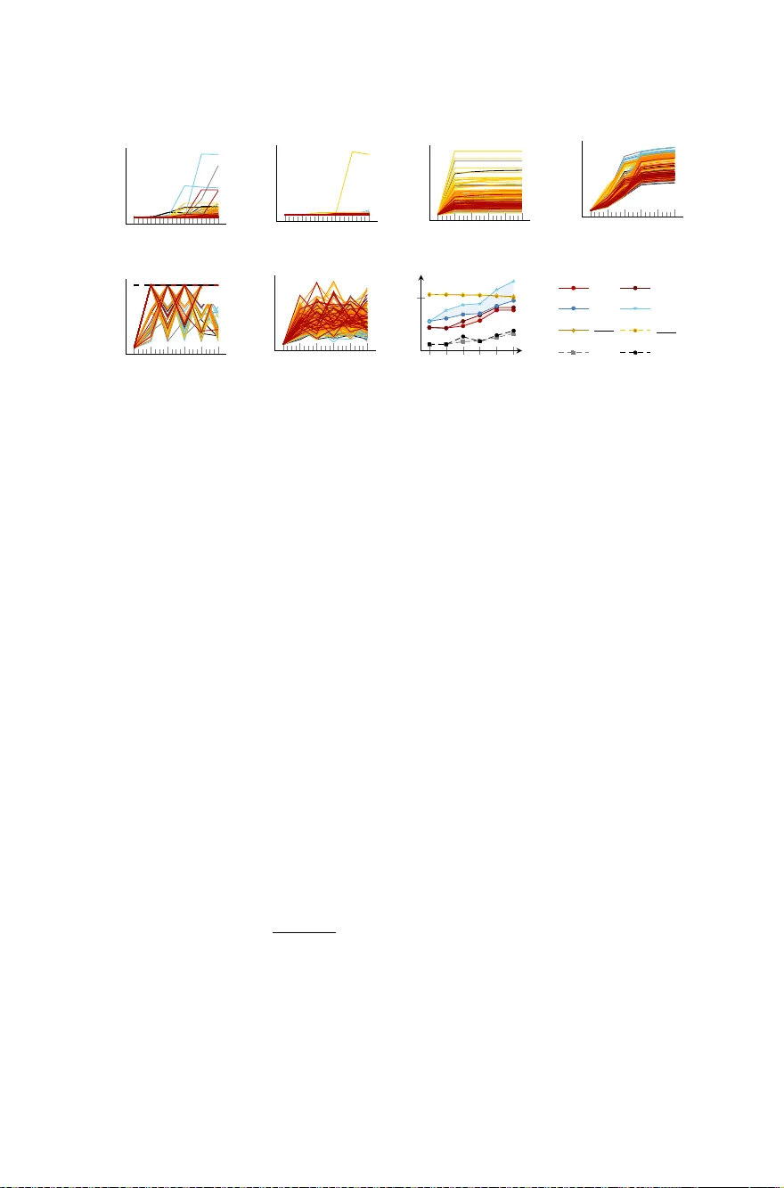
P ersisten t Homology as Stopping-Criterion for V oronoi In terp olation Luciano Melo dia [0000 − 0002 − 7584 − 7287] and Ric hard Lenz [0000 − 0003 − 1551 − 4824] Chair of Computer Science 6 F riedric h-Alexander Univ ersity Erlangen-N ¨ urn b erg 91058 Erl angen, Deutsc hland { luciano.melodia,richard.lenz } @fau.de Abstract. In this study the V oronoi in terp olation is used to inter- p olate a set of p oints drawn from a topological space with higher homology groups on its filtration. The technique is based on V oronoi tessellation, whic h induces a natural dual map to the Delaunay trian- gulation. Adv antage is tak en from this fact calculating the p ersistent homology on it after eac h iteration to capture the changing topol- ogy of the data. The b oundary p oin ts are identified as critical. The Bottlenec k and W asserstein distance serve as a measure of quality b et w een the original point set and the in terp olation. If the norm of tw o distances exceeds a heuristically determined threshold, the algorithm terminates. W e give the theoretical basis for this approach and justify its v alidity with n umerical exp erimen ts. Keyw ords: In terp olation · P ersistent homology · V oronoi triangula- tion 1 In tro duction Most in terp olation tec hniques ignore global prop erties of the underlying top ological space of a set of points. The topology of an augmented p oint set dep ends on the choice of in terp oland. How ever, it does not depend on the top ological structure of the data set. The V oronoi in terp olation is a technique considering these issues [ 3 ]. The algorithm has been inv ented b y Sibson [ 21 ]. Using V oronoi triangulation to determine the position of a new p oin t resp ects the topology in terms of simple-homotop y equiv alence. F or this an implicit restriction to a closed subset of the em b edded space is used, see Fig. 2. The closure of this subset dep ends on the metric, in Euclidean space it is flat. This restriction, also called clipping , leads to v arying results for interpolation according to the c hoice of clip. The clip do es not represent the intrinsic geometry nor the topology of the data, but that of the surrounding space. This leads to artifacts during in terp olation. P ersistent homology encodes the top ological prop erties and can be calcu- lated in high dimensions. Th us, it is used as indicator for such artifacts [ 25 ]. 2 L. Melodia, R. Lenz In particular, this measuremen t of top ological properties b ehav es stable, i.e. small changes in the coordinate function v alue also cause small c hanges in p ersisten t homology [ 9 ]. Efficien t data structures and algorithms ha ve b een designed to compute p ersisten t homology [ 25 , 24 ] and scalable w ays to compare p ersistence diagrams using the W asserstein metric ha v e b een dev elop ed [ 8 ]. This pap er uses persistent homology to decide whether a topological change o ccurs or not. Up to this p oin t it is an op en problem to detect these errors and to terminate the algorithm in time. Our contribution to a solution is divided in to three parts: – W e introduce p ersistent homology as a stopping-criterion for interpolation metho ds. The distance betw een t wo persistence diagrams is an indicator of top ological c hanges during augmen tation. – W e co ver the connection of the V oronoi tessellation to the Delaunay triangulation via dualit y . It is sho wn that the Delaunay complex is simple- homotop y equiv alent to the ˇ Cec h complex. W e further sho w that the Delauna y complex is sufficient to compute persistence diagrams. – W e in v estigate the method on a signature data set. It pro vides in teresting and visually in terpretable top ological features due to the topography of letters. Higher homology groups suc h as H 1 and H 2 ma y app ear on the filtration of a signature. This often represen ts an insurmoun table hurdle for other in terp olation tec hniques. 2 Simplicial Complexes and Filtrations T aking in to account the top ology of data is beneficial for interpolation, due to the assumption that the point set lies on a top ological or ev en smo oth manifold, ha ving a family of smooth co ordinate systems to describ e it. Another h yp othesis sa ys, that the mutual arrangemen t of ev ery dataset forms some ‘shap e’ [ 25 ], which c haracterizes the manifold. If the p oin t set changes its shap e, it is no longer iden tifiable with this manifold. Em b edded simplicial complexes, build out of a set of simplices, are suitable ob jects to detect such shapes, b y computing their homology groups. Simplices, denoted by σ , are the permuted span of the set X = { x 0 , x 1 , . . . , x k } ⊂ R d with k + 1 p oints, which are not contained in an y affine subspace of dimension smaller than k [19]. A simplex forms the con v ex hull σ := ( x ∈ X     k X i =0 λ i x i with k X i =0 λ i = 1 and λ i ≥ 0 ) . (1) Simplices are w ell-defined embeddings of p olyhedra. ‘Gluing’ simplices together at their fac es , we can construct simplicial complexes out of them. F aces are mean t to be h -dimensional simplices or h -simplices. Informally , the gluing T op ological Stopping for V oronoi In terpolation 3 creates a series of k -simplices, which are connected by h -simplices, that satisfy h < k . A finite simplicial complex denoted by K and em b edded into Euclidean space is a finite set of simplices with the prop erties, that each face of a simplex of K is again a simplex of K and the in tersection of tw o simplices is either empt y or a common face of b oth [19]. W e w ant to tak e in to account the systematic dev elopment of a simplicial complex up on a point cloud. This is called filtration and it is the decomp osition of a finite simplicial complex K in to a nested sequence of sub-complexes, starting with the empt y set [10]: ∅ = K 0 ⊂ K 1 ⊂ · · · ⊂ K n = K, (2) K t +1 = K t ∪ σ t +1 , for t ∈ { 0 , . . . , n − 1 } . (3) In practice a parameter r is fixed to determine the step size of the nested complexes. This can be though t as a ‘lens’ zo oming in to a certain ‘gran ularit y’ of the filtration. In the following, we presen t four different simplicial complexes and their theoretical connection. 2.1 ˇ Cec h Complex Let the radius r ≥ 0 b e a real n um b er and B ( x, r ) = { y ∈ R d | || x − y || ≤ r } the closed ball centered around the p oin t x ∈ X ⊆ R d . The ˇ Cec h complex for a finite set of p oin ts X is defined as ˇ Cec h( X , r ) = { U ⊆ X | \ x ∈ U B ( x, r ) 6 = ∅} . (4) By || · || w e denote consequently the L 2 -norm. In terms of abstract simplicial complexes (see sec. 7), the ˇ Cec h complex is the full abstract simplex spanned o ver X [ 2 ]. According to the Nerv e lemma it is homotop y-equiv alen t to the union of balls B ( X, r ) = S x ∈ U B ( x, r ) [ 7 ]. Spanning the simplicial complex for r = sup x,y ∈ U || x − y || , we get the full simplex for the set U . F or t wo radii r 1 < r 2 w e get a nested sequence ˇ Cec h ( X, r 1 ) ⊂ ˇ Cec h ( X, r 2 ). This implies that the ˇ Cec h complex forms a filtration o ver U and therefore a filtration o ver the topological space X if U = X [ 2 ]. These properties make the ˇ Cec h complex a very precise descriptor of the top ology of a p oin t set. The flip side of the coin is that the ˇ Cec h complex is not efficien tly computable for large p oin t sets. A related complex is therefore presen ted next, which is sligh tly easier to compute. 2.2 Vietoris-Rips Complex The Vietoris-Rips complex Rips ( X, r ) with v ertex set X and distance threshold r is defined as the set Rips( X, r ) =  U ⊆ X     || x − y || ≤ r, for all x, y ∈ U  . (5) 4 L. Melodia, R. Lenz Fig. 1. F our of fiv e geometric complexes app earing in the collapsing sequence of the ˇ Cec h-Delaunay Collapsing Theorem [ 2 ]. F rom left to right : A high dimensional ˇ Cec h complex pro jected onto the plane, the ˇ Cec h-Delaunay complex, the Delaunay complex, the Witness complex, whic h is an outlier in the ro w due to the c hanging shap e b y differen t Witness sets (white bullets) and the W rap complex. The Vietoris-Rips complex requires only the comparison of distance me asures to b e obtained. It spans the same 1-skeleton as the ˇ Cec h complex and fulfills for an em b edding in to any metric space the follo wing relationship [ 5 , p. 15]: Rips ( X, r ) ⊆ ˇ Cec h ( X, r ) ⊆ Rips ( X, 2 r ) . T o see this, we c ho ose a simplex σ = { x 0 , x 1 , . . . , x k } ∈ Rips ( X, r ). The point x 0 ∈ T k i =0 B ( x i , r ) must b e within the intersection of closed balls with radius r of all p oin ts. Now w e c ho ose a σ = { x 0 , x 1 , . . . , x k } ∈ ˇ Cec h ( X, r ), then there is a p oin t y ∈ R d within the intersection y ∈ T k i =0 B ( x i , r ), which is the desired condition d ( x i − y ) ≤ r for any i = 0 , . . . , k . Therefore, for all i, j ∈ { 0 , . . . , k } the follo wing (in)equality applies: d ( x i − x j ) ≤ 2 r and σ ∈ Rips( X, 2 r ). The calculation time for the Vietoris-Rips complex is b etter than for the ˇ Cec h complex, with a b ound of O ( n 2 ) for n p oin ts [ 24 ]. As a third complex w e introduce the α -complex or Delaunay complex, for whic h the definition of V oronoi cells and balls are prerequisite. 2.3 Delauna y Complex If X ⊂ R d is a finite set of points and x ∈ X , then the V oronoi cell or also V oronoi region of a p oint x ∈ X is given by V or( x ) =  y ∈ R d     || y − x || ≤ || y − z || , for all z ∈ X  . (6) The V oronoi ball of x with resp ect to X is defined as the in tersection of the V oronoi region with the closed ball of given radius around this p oin t, i.e. V orBall ( x, r ) = B ( x, r ) ∩ V or ( x ) [ 2 ].The Delauna y complex on a point set X is defined as Del( X, r ) = ( U ⊆ X     \ x ∈ U V orBall( x, r ) 6 = ∅ ) . (7) T op ological Stopping for V oronoi In terpolation 5 There is a fundamen tal connection b et ween the union of all V oronoi balls o ver X and the Delauna y complex. The idea is to find a go o d c over that do es represen t the global topology . T aking the top ological space X and U = S i ∈ I U i b eeing an op en cov er, w e define the Nerv e of a co v er as its top ological structure. Therefore, the empt y set ∅ ∈ N ( U ) is part of the Nerv e and if T j ∈ J U j 6 = ∅ for a J ⊆ I , then J ∈ N ( U ). W e consider U to b e a go od cov er, if for eac h σ ⊂ I the set T i ∈ σ U i 6 = ∅ is contractible, or in other words if it has the same homotopy type as a point. In this case the Nerv e N ( U ) is homotop y equiv alent to S i ∈ I U i . Most interestingly , the Delaunay complex Del r ( X ) of a p oin t set X is isomorphic to the Nerve of the collection of V oronoi balls. T o see this, w e construct V oronoi regions for tw o different sets. Th us, we denote the V oronoi region V or ( x, r , U ) of a p oint within a set U . Be V or ( x, r , U ) ⊆ V or ( x, r , V ) for eac h op en set U ⊆ V ⊆ X and all x ∈ X . W e obtain the largest V oronoi ball for U = ∅ and the smallest V oronoi ball for U = X . In the first case each region is a ball with radius r and in the second case the V oronoi balls form a con vex decomposition of the union of balls. W e select a subset U and restrict the Delauna y complex to it b y taking in to accoun t only the V oronoi balls around the p oin ts in U . It is called selective Delauna y complex and con tains the Delauna y and ˇ Cec h complex in its extremal cases: Del( X, r, U ) = ( V ⊆ X     \ x ∈ V V orBall( x, r, U ) 6 = ∅ ) . (8) Since the union of op en balls does not dep end on U , the Nerv e lemma implies, that for a giv en set of poin ts X and a radius r all selectiv e Delauna y complexes ha ve the same homotop y type. This also results in Del ( X, r, V ) ⊆ Del ( X, s, U ) for all r ≤ s and U ⊆ V . The pro of has b een giv en first b y [2, § 3.4]. 2.4 Witness Complex Through the restriction of the faces to randomly chosen subsets of the point cloud the filtration is carried out on a scalable complex, which is suitable for large p oin t sets. W e call these subsets Witnesses W ⊂ R d and L ⊂ R d landmarks. The landmarks can be part of the Witnesses L ⊆ W , but do not ha ve to. Then σ is a simplex with vertices in L and some p oin ts w ∈ W . W e sa y that w is Witnessed by σ if || w − p || ≤ || w − q || , for all p ∈ σ and q ∈ L \ σ . W e further say it is strongly Witnessed by σ if || w − p || ≤ || w − q || , for all p ∈ σ and q ∈ L . The Witness complex Wit ( L, W ) consists of all simplices σ , suc h that any simplex ˜ σ ⊆ σ has a Witness in W and the strong Witness complex analogously . The homology groups of the Witness complex dep end strongly on the landmarks. In addition to equally distributed initialization, strategies suc h as sequen tial MaxMin can lead to a more accurate estimate of homology groups [22]. Its time b ound for construction is O ( | W | log | W | + k | W | ) [5]. 6 L. Melodia, R. Lenz 3 P ersisten t Homology Theory W e are particularly in terested in whether a top ological space can b e con tin u- ously transformed in to another. F or this purpose its k -dimensional ‘holes’ pla y a cen tral role. Given tw o topological spaces M and N w e sa y that they ha ve the same homotopy typ e , if there exists a contin uous map h : M × I → N , which deforms M o ver some time in terv al I in to N . But it is v ery difficult to obtain homotopies. An algebraic w a y to compute something strongly related is ho- mology . The connection to homotop y is established b y the Hurewicz Theorem. It sa ys, that given π k ( x, X ), the k -th homotop y group of a topological space X in a point x ∈ X , there exists a homomorphism h : π k ( x, X ) → H k ( x, X ) in to the k -th homology group at x . It is an isomorphism if X is ( n − 1)- connected and k ≤ n when n ≥ 2 with abelianization for n = 1 [ 17 ]. In this particular case, we are able to use an easier to calculate in v ariant to describ e the top ological space of the data up to homotop y . F urther we need to define what a b oundary and what a c hain is, resp ectiv ely . W e wan t to describ e the b oundary of a line segmen t by its t w o endp oin ts, the b oundary of a triangle, or 2-simplex by the union of the edges and the b oundary of a tetrahedron, or 3-simplex b y the union of the triangular faces. F urthermore, a b oundary itself shall not hav e a b oundary of its own. This implies the equiv alence of the prop ert y to b e b oundaryless to the concept of a ‘lo op’, i.e. the p ossibilit y to return from a starting p oin t to the same point via the k -simplices, by not ‘en tering’ a simplex twice and not ‘lea ving’ a simplex ‘unentered’. Let σ k b e a k -simplex of a simplicial complex K := K ( X ) ov er a set of p oin ts X . F urther, let k ∈ N . The linear com binations of k -simplices span a v ector space C k := C k ( K ) = span  σ k 1 , . . . , σ k n  . This v ector space is called k -th c hain group of K and con tains all linear com binations of k -simplices. The coefficients of the group lie in Z and the group structure is established b y ( C k , +), with e C k = 0 b eing the neutral element and addition as group op eration. A linear map ∂ : C k → C k − 1 is induced from the k -th chain group in to the ( k − 1)-th. The b oundary operator ∂ k ( σ k ) : C k → C k − 1 is defined b y ∂ k ( σ k ) = k X i =0 ( − 1) i ( v 0 , . . . , b v i , . . . , v k ) . (9) The v ertex set of the k -simplex is v 0 , . . . , v k . This group homomorphism con tains an alternating sum, th us for eac h oriented k -simplex ( v 0 , . . . , v k ) one elemen t b v i is omitted. The boundary operator can be comp osed ∂ 2 := ∂ ◦ ∂ . W e observ e, that every c hain, which is a boundary of higher-dimensional chains, is b oundaryless. An ev en comp osition of boundary maps is zero ∂ 2 Z = 0 [ 17 ]. The k ernel of ( C k , +) is the collection of elemen ts from the k -th c hain group mapp ed b y the boundary op erator to the neutral elemen t of ( k − 1)-th: k er ∂ k = ∂ − 1 k ( e C k − 1 ) = { σ k ∈ C k | ∂ k ( σ k ) = e C k − 1 } . A cycle should b e defined b y having no b oundary . F rom this we get a group of k -cycles, denoted by Z k , whic h is defined as the k ernel of the k -th boundary operator Z k := k er ∂ k ⊆ C k . T op ological Stopping for V oronoi In terpolation 7 Ev ery k -simplex mapp ed to zero by the boundary op erator is considered to b e a cycle and the collection of cycles is the group of k -cycles Z k . The k - b oundaries are therefore B k = Im ∂ k +1 ⊂ Z k . The k -th homology group H k is the quotien t H k := Z k /B k = k er ∂ k / Im ∂ k +1 . (10) W e compute the k -th Betti num b ers b y the rank of this vector space, i.e. β k = rank H k . In a certain sense the Betti num b ers count the amount of holes in a top ological space, i.e. β 0 coun ts the connected comp onents, β 1 the tunnels, β 2 v oids and so forth. Using Betti n umbers, the homology groups can b e trac k ed along the filtration, representing the ‘birth’ and ‘death’ of homology classes. The filtration of a simplicial complex defines a sequence of homology groups connected by homomorphisms for eac h dimension. The k -th homology group o ver a simplicial complex K r with parameter r is denoted b y H r k = H k ( K r ). This gives a group homomorphism g r,r +1 k : H r k → H r +1 k and the sequence [15]: 0 = H 0 k g 0 , 1 k − − → H 1 k g 1 , 2 k − − → · · · g n,r k − − − → H r k g r,r +1 k − − − − → H r +1 k = 0 . (11) The image Im g r,r +1 k consists of all k -dimensional homology classes which are b orn in the K r -complex or app ear b efore and die after K r +1 . The dimension k p ersisten t homology group is the image of the homomorphisms H n,r k = Im g n,r k , for 0 ≤ n ≤ r ≤ r + 1 [ 15 ]. F or each dimension there is an index pair n ≤ r . T racking the homology classes in this wa y yields a m ulti set, as elements from one homology group can appear and v anish sev eral times for a certain parametrization. Th us, we get the follo wing multiplicit y: µ n,r k = ( β n,r − 1 k − β n,r k ) | {z } Birth in K r − 1 , death at K r . − ( β n − 1 ,r − 1 k − β n − 1 ,r k ) | {z } Birth b efore K r , death at K r . (12) The first difference counts the homology classes born in K r − 1 and dying when K r is entered. The second difference counts the homology classes b orn before K r − 1 and dying by entering K r . It follows that µ n,r k coun ts the k -dimensional homology classes b orn in K n and dying in K r [15]. The persistence diagram for the k -th dimension, denoted as P (dim k ) K , is the set of p oin ts ( n, r ) ∈ ¯ R 2 with µ n,r k = 1 where ¯ R := R ∪ + ∞ . W e define the general p ersisten t diagram as the disjoint union of all k -dimensional p ersistence diagrams P K = F k ∈ Z P (dim k ) K . In this pap er w e consider H 0 , H 1 and H 2 . W e now in tro duce distances for comparison of p ersistence diagrams. In particular, it is important to resolve the distance b et ween m ultiplicities in a meaningful w ay . Note that they are only defined for n < r and that no v alues app ear below the diagonal. This is to b e interpreted suc h that a homology class can’t disapp ear before it arises. 8 L. Melodia, R. Lenz 4 Bottlenec k Distance Let X b e a set of p oin ts embedded in Euclidean space and K 1 r , K 2 r t wo simplicial complexes forming a filtration o ver X . Both are finite and ha ve in all their sub-level sets homology groups of finite rank. Note, that these groups c hange due to a finite set of homology-critical v alues. T o define the b ottlenec k distance w e use the L ∞ -norm || x − y || ∞ = max {| x 1 − y 1 | , | x 2 − y 2 |} b et w een t wo p oin ts x = ( x 1 , x 2 ) and y = ( y 1 , y 2 ) for x ∈ P K 1 and y ∈ P K 2 . By con ven tion, it is assumed that if x 2 = y 2 = + ∞ , then || x − y || ∞ = | x 1 − y 1 | . If P K 1 and P K 2 are tw o p ersistence diagrams and x := ( x 1 , x 2 ) ∈ P K 1 and y := ( y 1 , y 2 ) ∈ P K 2 , resp ectiv ely , their Bottleneck distance is defined as d B ( P K 1 , P K 2 ) = inf ϕ sup x ∈P K 1 || x − ϕ ( x ) || ∞ , (13) where ϕ is the set of all bijections from the multi set P K 1 to P K 2 [5]. 4.1 Bottleneck Stabilit y W e consider a smooth function f : R → R as a w orking example. A p oin t x ∈ R of this function is called critical and f ( x ) is called critical v alue of f if d f x = 0. The critical p oin t is also said to b e not degenerated if d 2 f x 6 = 0. Im f ( x ) is a homology critical v alue, if there is a real n um b er y for whic h an integer k exists, such that for a sufficien tly small α > 0 the map H k  f − 1 (( −∞ , y − α ])  → H k  f − 1 (( −∞ , y + α ])  is not an isomorphism. W e call the function f tame if it has a finite n umber of homology critical v alues and the homology group H k  f − 1 (( −∞ , y ])  is finite-dimensional for all k ∈ Z and y ∈ R . A p ersistence diagram can be generated by pairing the critical v alues with each other and transferring corresponding p oints to it. The Bottleneck distance of the p ersistence diagram of t wo tame functions f , g is restricted to a norm b et ween a p oin t and its bijective pro jection. Therefore, not all p oin ts of a multi se t can be mapp ed to the nearest point in another [ 12 ]. T o see this, we consider f to be tame. The Hausdorff distance d H ( X, Y ) b et w een tw o multi sets X and Y is defined by max  sup x ∈ X inf y ∈ Y || x − y || ∞ , sup y ∈ Y inf x ∈ X || y − x || ∞  . (14) F rom the results of [ 9 ] it is kno wn that the Hausdorff (in)equality d H ( P f , P g ) ≤ || f − g || ∞ = α holds and that there must exist a p oin t ( x 1 , x 2 ) ∈ P f whic h has a maximum distance α to a second p oin t ( y 1 , y 2 ) ∈ P g . In particular, ( y 1 , y 2 ) m ust b e within the square [ x 1 − α, x 1 + α ] × [ x 2 − α, x 2 + α ]. Let x 1 ≤ x 2 ≤ x 3 ≤ x 4 b e p oin ts in the extended plane ¯ R 2 . F urther, let R = [ x 1 , x 2 ] × [ y 1 , y 2 ] b e a square and R α = [ x 1 + α, x 2 − α ] × [ y 1 + α, y 2 − α ] another shrink ed square b y some parameter α . Thus, w e yield # ( P f ∩ R α ) ≤ # ( P g ∩ R ) . (15) T op ological Stopping for V oronoi In terpolation 9 W e need the inequality to find the smallest α suc h that squares of side-length 2 α cen tered at the p oin ts of one diagram co ver all off-diagonal elements of the other diagram, and vice v ersa with the diagrams exchanged [ 12 ]. The p ersistence diagrams P f and P g satisfy for tw o tame functions f , g : X → R : d B ( P f , P g ) ≤ || f − g || ∞ . (16) W e take tw o points x = ( x 1 , x 2 ) , y = ( y 1 , y 2 ) ∈ P f and look at the infinite norm betw een them in the p ersistence diagram of f outside the diagonal ∆ . In case that there is no suc h second p oin t we consider the diagonal itself: δ f = min {|| x − y || ∞ | P f − ∆ 3 x 6 = y ∈ P f } . (17) W e c ho ose a second tame function g , which satisfies || f − g || ∞ ≤ δ f / 2. W e cen ter a square R α ( x ) at x with radius α = || f − g || ∞ . Applying Eq. 15 yields µ ≤ #( P g ∩ R α ( x )) ≤ #( P f ∩ R ( x ) 2 α ) . (18) Since g w as chosen in such a wa y , that || f − g || ∞ ≤ δ f / 2 applies, w e conclude that 2 α ≤ δ f . Thus, x is the only p oin t of the p ersistence diagram P f that is inside R 2 α and the m ultiplicity µ is equal to #( P g ∩ R ( x ) α ). W e can now pro ject all points from P g in R ( x ) α on to x . As d H ( P f , P g ) ≤ α holds, the remaining p oin ts are mapp ed to their nearest point on the diagonal. 5 W asserstein Distance The W asserstein distance is defined for separable completely metrizable top o- logical spaces. In this particular case b etw een the t w o p ersistence diagrams P K 1 and P K 2 . The L p -W asserstein distance W p is a metric arising from the examination of transp ort plans b et ween t w o distributions and is defined for a p ∈ [1 , ∞ ) as d W p ( P K 1 , P K 2 ) =   inf ϕ X x ∈P K 1 || x − ϕ ( x ) || p ∞   1 /p . (19) Then ϕ : P K 1 → P K 2 is within the set of all transp ortation plans from P K 1 to P K 2 o ver P K 1 × P K 2 . W e use the L 1 -W asserstein distance. The W asserstein distance satisfies the axioms of a metric [ 23 , p. 77]. The transp ortation problem can b e stated as finding the most economical w a y to transfer the points from one p ersistence diagram in to another. W e assume that these tw o p ersistence diagrams are disjoint subsets of ¯ R 2 × ¯ R 2 . The cost of transport is given b y d : ¯ R 2 × ¯ R 2 → [0 , ∞ ), so that || x − ϕ ( x ) || indicates the length of a path. The transport plan is then a bijection ϕ : P K 1 → P K 2 from one persistence diagram to the other. The W asserstein distance of t w o p ersistence diagrams is the optimal cost of all transp ort plans. Note, that the L ∞ -W asserstein distance is equiv alent to the Bottlenec k distance, i.e. d B is the limit of d W p as p → ∞ . 10 L. Melo dia, R. Lenz Fig. 2. F rom left to right : Clipp ed tessellation. F or other manifolds the curv ature should be considered; T essellation with added p oin t creates a new V oronoi region ste aling area from the neigh b oring regions; The determined w eights b y the fractional amoun t of occupied area; T essellation with added p oin t. 5.1 W asserstein Stability The distance d W p is stable in a trianguliable compact metric space, whic h restricts it to Lipsc hitz con tinuous functions for stable results. A function f : X → Y is called Lipschitz con tin uous, if one distance ( X, d X ) is b ounded b y the other ( Y , d Y ) times a constan t, i.e. d Y ( f ( x 1 ) − f ( x 2 )) ≤ c · d X ( x 1 − x 2 ), for all x 1 , x 2 ∈ X. F or t wo Lipschitz functions f , g constan ts b and c exist [ 13 ], whic h dep end on X and the Lipschitz constants of f and g , suc h that the p -th W asserstein distance b etw een the t wo functions satisfies d W p ( f , g ) ≤ c · || f − g || 1 − b/p ∞ . (20) F or small enough perturbations of Lipschitz functions their p -th W asserstein distance is b ounded by a constant. In Fig. 3 the top ological developmen t of handwritings through in terp olation is visualized. Equally colored lines represen t the same user and each line represen ts a signature. The equally colored lines show v ery similar b ehavior and represen t the small p erturbations, whic h are caused by the sligh t c hange of letter shap e when signing m ultiple times. 6 The Natural Neigh b or Algorithm The algorithm re-weigh ts the co ordinates of a new p oin t in the conv ex h ull of a point cloud b y the c hange of V oronoi regions relativ e to the V oronoi regions without the additional p oin t, i.e. ˆ x • = P L l =1 λ l x • l . F or a set of p oin ts X ⊂ R d distributed ov er an embedded manifold M natural neighbors b eha ve lik e a lo cal coordinate system for M with their density increasing [4]. The V oronoi tessellation is dual to the Delaunay triangulation, th us w e use the latter for our computation [ 6 , pp. 45-47]. This dualit y giv es a bijec- tion betw een the faces of one complex and the faces of the other, including incidence and reversibilit y of op erations. Both hav e the same homotopy t yp e. T op ological Stopping for V oronoi In terpolation 11 A V oronoi diagram dgm V or ( X ) is defined b y the union of the V oronoi re- gions dgm V or ( X ) := S x ∈ X V or ( x ) , for all x ∈ X and assigns a p olyhedron to eac h p oin t, see Fig. 2. This in terp olation method generalizes to arbitrary dimensions. The com binatorial complexit y of the V oronoi diagram of n p oin ts of R d is at most the combinatorial complexity of a polyhedron defined as the intersection of n half-spaces of R d +1 . Due to duality the construction of dgm V or ( X ) takes O ( n log n + n d/ 2 ) [6]. 6.1 V oronoi T essellation The V oronoi cells hav e no common interior, in tersect at their boundaries and co ver the en tire R d . The resulting p olygons can then b e divided into V oronoi edges and v ertices. The natural neigh b ors of a p oin t are defined b y the points of the neigh b oring V oronoi p olygons [21]. The natural neighbor is the closest point x to tw o other p oin ts y and z within X . T o yield the p osition of the added point we ha ve to calculate the V oronoi diagram of the original signature dgm V or ( X ) and one with an added p oin t dgm • V or ( X ∪ x • ) = S x ∈ X ∪ x • V or ( x ). The latter consists of one V oronoi region more than the primer, see Fig. 2 (a) and (c). This p olygon is part of dgm • V or ( X ∪ x • ) and con tains a certain amount of its ‘area’. The V oronoi regions sum up to one P L l =1 λ l = 1. The V oronoi in terpolation is rep eated un til the topological stopping condition is met, measured through the W p -distances of the persistence diagrams P K and P K • . The w eights of the coordinate representation of x • are determined b y the quotien t of the ‘stolen’ V oronoi regions and the total ‘area’ of the V oronoi diagram with the additional p oin t according to Eq. 21 [1]. λ l = ( vol(V or( x l ) ∩ V or • ( x • )) vol(V or • ( x • )) if x ≥ 1 , 0 otherwise. (21) But to what exten t are homology groups preserved if persistent homology is computed on the Delauna y triangulation? 7 The Simplicial Collapse The Delaunay triangulation av oids the burden of an additional simplicial structure for p ersisten t homology . W e determine how accurate the p ersis- ten t homology is on this filtration. W e use results from simplicial collapse [ 2 ], which show the simple-homotopy equiv alence of the ˇ Cec h and Delau- na y complex among other related simplicial complexes. Simple-homotop y equiv alence is stronger than homotop y equiv alence. An elemen tary simplicial collapse determines a strong deformation retraction up to homotop y . Hence, simple-homotop y equiv alence implies homotop y equiv alence [ 11 , § 2]. Under 12 L. Melo dia, R. Lenz the conditions of the Hurewicz Theorem we can dra w conclusions about the homotop y groups of the data manifold. The simplicial collapse is established using abstract simplicial complexes denoted b y ˜ K . A family of simplices σ of a non-empty finite subset of a set ˜ K is an abstract simplicial complex if for ev ery set σ 0 in σ and every non-empt y subset σ 00 ⊂ σ 0 the set σ 00 also belongs to σ . W e assume σ and σ 0 are t wo simplices of ˜ K , such that σ ⊂ σ 0 and dim σ < dim σ 0 . W e call the face σ 0 free, if it is a maximal face of ˜ K and no other maximal face of ˜ K con tains σ . A similar notion to deformation retraction needs to b e defined for the in vestigation of homology groups. This leads to the simplicial collapse & of ˜ K , whic h is the remo v al of all σ 00 simplices, where σ ⊆ σ 00 ⊆ σ 0 , with σ b eing a free face. No w we can define the simple-homotopy t yp e based on the concept of simplicial collapse. Intuitiv ely sp eaking, t w o simplicial complexes are ‘com binatorial-equiv alen t’, if it is p ossible to deform one complex in to the other with a finite n umber of ‘mov es’. Tw o abstract simplicial complexes ˜ K and ˜ G are said to hav e the same simple-homotopy type, if there exists a finite sequence ˜ K = ˜ K 0 & ˜ K 1 & · · · & ˜ K n = ˜ G , with eac h arrow represen ting a simplicial collapse or expansion (the inv erse op eration). If X is a finite set of p oin ts in general p osition in R d , then ˇ Cec h( X , r ) & Del ˇ Cec h( X , r ) & Del( X , r ) & W rap( X , r ) (22) for all r ∈ R . F or the pro of w e refer to [ 2 ]. The connection in Eq. 22 establishes the simple-homotopy equiv alence of the ˇ Cec h- and Delaunay complex. W e deduce, that if the underlying space follo ws the condition of a Hurewicz iso- morphism, all four complexes are suitable for calculating p ersisten t homology as a result of the simplicial collapse up to homotopy e quiv alence. 8 Numerical Exp erimen ts All source co de is written in Python 3.7. The GUDHI [ 16 ] library is used for the calculation of simplicial complexes, filtrations and p ersisten t homology . W e inv estigate 83 users, considering 45 signatures p er user from the MOBISIG signature database [ 18 ], whic h show the same letters, but are independent writings. F or eac h user w e hav e a set of 45 p ersistence diagrams and a set of 45 corresponding handwritings. In every iteration as man y new p oin ts are added as are already in the resp ective example of a signature. W e inserted the p oin ts uniformly within the con v ex hull of the initial p oin t set, see Fig. 2. 8.1 Exp erimen tal Setting Rips ( X ) is expanded up to the third dimension. The maximum e dge length is set to the a verage edge length b etw een tw o p oin ts within the data set. W e use the same r for ˇ Cec h ( X, r ) and Rips ( X, r ), so that Rips ( X, r ) differs top ologically more from the union of closed balls around each p oint, but T op ological Stopping for V oronoi In terpolation 13 t 0 t 1 t 2 t 3 t 4 t 5 d B ( P t Del , P t +1 Del ) t 0 t 1 t 2 t 3 t 4 t 5 d W 1 ( P t Del , P t +1 Del ) t 0 t 1 t 2 t 3 t 4 t 5 d B ( P t Rips , P t +1 Rips ) t 0 t 1 t 2 t 3 t 4 t 5 d W 1 ( P t Rips , P t +1 Rips ) t 0 t 1 t 2 t 3 t 4 t 5 ∞ d B ( P t Wit , P t +1 Wit ) t 0 t 1 t 2 t 3 t 4 t 5 d W 1 ( P t Wit , P t +1 Wit ) t 0 t 1 t 2 t 3 t 4 t 5 0 . 8 µ X ˜ µ X σ X ˜ σ X σ X µ X ˜ σ X ˜ µ X w 1 ˜ w 1 Fig. 3. Bottlenec k and L 1 -W asserstein distances b et ween the p ersistence diagrams in iteration t and t + 1. The persistent homology has b een computed on the Delaunay complex, Vietoris-Rips complex and the witness complex, resp ectiv ely . A total of 250 samples from a signature collection are represented [ 18 ]. Each line corresp onds to a single sample and the lines are colored corresp onding to one of six selected users in • gra y , • blac k, • blue, • y ellow, • orange and • red. is faster to compute. Finding an optimal radius as distance threshold is considered op en [ 25 ], thus we use r = max x,y ∈ X || x − y || as empirical heuristic. The strong Wit ( X, r ), embedded into R d , is recalculated for each sample at eac h in terpolation step. W e select uniformly 5% of the p oin ts as landmarks. W e set α = 0 . 01 , γ = 0 . 1 and p = 1. W e assume that the p ersistence diagrams are i.i.d. A free parameter α quan tifies a tolerance to topological c hange, thus a decision m ust b e made on the following h ypotheses about the distributions of the p ersistence diagrams: (a) H 0 : P t K and P t +1 K ha ve differen t underlying distributions and (b) H 1 : P t K and P t +1 K ha ve the same underlying distribution. W e use an asymptotic solution for testing b y trimmed W asserstein distance [14]: ˆ Γ p γ ( P t K , P t +1 K ) = 1 (1 − 2 γ )   m X j =1 || ( P t K ) j − P t +1 K ) j || p ∞ ∆γ   1 /p . (23) The trimming b ound α ∈ [0 , 1 / 2) results from the integral for the contin uous case as a difference in a finite w eighted sum. It is computed using the expected v alue of the p ersistence diagrams and is exact in the limit R 1 − γ γ f ( x ) dx = lim ∆γ → 0 P x ∈ X f ( x ) ∆γ . The critical region for our h yp othesis H 0 against H 1 14 L. Melo dia, R. Lenz is  nm n + m  1 p ˆ Γ p γ − α p ˆ σ γ ≤ z γ , (24) where z γ denotes the γ -quan tile of the standard normal distribution and n = m , with n b eing the n umber of samples. The initial problem can b e rephrased as (a) H 0 : Γ p γ ( P t K , P t +1 K ) > α and (b) H 1 : Γ p γ ( P t K , P t +1 K ) ≤ α . 8.2 Ev aluation In Fig. 3, seven th diagram, elemen tary statistics are computed for the en tire data set suc h as mean µ X , standard deviation σ X , v ariation σ X µ X and d W 1 = d W 1 ( X org , X t ). The statistics are also computed for the interpolated data with top ological stop, respectively , marked with ∼ . W e ac hiev ed an impro v ement for eac h measured statistic at eac h iteration step using topological stop. In Fig. 3 the top ological similarit y betw een the individual users are made visual. Rips ( X, r ) and Del ( X, r ) seem suitable to estimate the homology groups, whereas Wit ( L, W ) produced far less stable results, due to the small selection of landmarks. 9 Conclusions W e ha ve discussed the connection of V oronoi diagrams to the Delaunay complex and its connection to other complexes, which should serve as a basis to explore related algorithms to the V oronoi interpolation. W e inv estigated in to metrics to measure differences in p ersisten t homology and could visualize the changing homology groups of the users signatures during in terp olation, see Fig. 3. Our result is a stopping-criterion with a hypothesis test to determine whether the p ersisten t homology of an interpolated signature still originates from the same distribution as the source. Our measurements sho w an improv emen t of statistics compared to v anilla V oronoi interpolation. W e demonstrated, that – under mild conditions – the Delaunay complex, ˇ Cec h-Delaunay complex and W rap complex can also b e used for filtration up to homotopy equiv alence. F ollowing open research questions arose during our in vestigations: – The in trinsic geometry of the data p oints is often not the Euclidean one. On the other hand side the frequen tly used embedding of the V oronoi tessellation is. This causes un w anted artifacts. Is there a geometrically meaningful clipping for general metric spaces, for example using geo desics in a smooth manifold setting? In whic h manifold should Del ( X ) be em- b edded? T op ological Stopping for V oronoi In terpolation 15 – T o our kno wledge there is no evidence known that the V oronoi tessellation obtains the homology groups. According to [ 20 ], the V oronoi tessellation is stable. Ho wev er, the experiments show that for increasing iterations additional homology groups appear. Do es the V oronoi tessellation preserv e homology groups and homotop y groups in general metric spaces? Ac knowledgemen ts. W e would lik e to thank Da vid Haller and Lekshmi Beena Gopalakrishnan Nair for pro ofreading. F urther, we thank An ton Rec henauer, Jan F rahm and Justin No el for suggestions and ideas on the elab oration of the final version of this w ork. W e express our gratitude to Demian V¨ ohringer and Melanie Sigl for p oin ting out related work. This w ork w as partially supp orted b y Siemens Gas and Po wer Gm bH & Co. K G. Co de & Data. The implemen tation of the metho ds, the data sets and exp erimen tal results can be found at: https://gith ub.com/k arh unenlo ev e/ SIML . References 1. An ton, F., Mio c, D., F ournier, A.: Reconstructing 2d images with natural neigh b our interpolation. The Visual Computer 17(3), 134–146 (2001) 2. Bauer, U., Edelsbrunner, H.: The morse theory of ˇ cec h and delaunay complexes. T ransactions of the American Mathematical Society 369(5), 3741–3762 (2017) 3. Bobac h, T.A.: Natural Neigh b or Interpolation - Critical Assessment and New Con tributions. Doctoral thesis, TU Kaiserslautern (2009) 4. Boissonnat, J., Cazals, F.: Natural neigh b or co ordinates of points on a surface. Computational Geometry 19(2-3), 155–173 (2001) 5. Boissonnat, J.D., Chazal, F., Yvinec, M.: Geometric and T op ological Inference, v ol. 57. Cambridge Universit y Press (2018) 6. Boissonnat, J.D., Dy er, R., Ghosh, A.: Delauna y triangulation of manifolds. F oundations of Computational Mathematics 18(2), 399–431 (2018) 7. Borsuk, K.: On the im b edding of systems of compacta in simplicial complexes. F undamen ta Mathematicae 35, 217–234 (1948) 8. Carri ` ere, M., Cuturi, M., Oudot, S.: Sliced w asserstein k ernel for p ersistence diagrams. In: Pro ceedings of the 34th International Conference on Machine Learning. pp. 664–673 (2017) 9. Cerri, A., Landi, C.: Hausdorff stability of p ersistence spaces. F oundations of Computational Mathematics 16(2), 343–367 (2016) 10. Chazal, F., Glisse, M., Labru` ere, C., Mic hel, B.: Conv ergence rates for p ersistence diagram estimation in top ological data analysis. Journal of Mac hine Learning Researc h 16, 3603–3635 (2015) 11. Cohen, M.: A Course in Simple-Homotopy Theory , v ol. 10. Springer (2012) 12. Cohen-Steiner, D., Edelsbrunner, H., Harer, J.: Stability of p ersistence diagrams. Discrete a nd Computational Geometry 37(1), 103–120 (2007) 16 L. Melo dia, R. Lenz 13. Cohen-Steiner, D., Edelsbrunner, H., Harer, J., Mileyko, Y.: Lipsc hitz functions ha ve lˆp-stable persistence. F oundations of Computational Mathematics 10(2) (2010) 14. Czado, C., Munk, A.: Assessing the similarity of distributions-finite sample p er- formance of the empirical mallo ws distance. Journal of Statistical Computation and Si mulation 60(4), 319–346 (1998) 15. Edelsbrunner, H., Harer, J.: Persisten t homology – a survey . Con temp orary mathematics 453, 257–282 (2008) 16. Gh udi user and reference manual, http://gudhi.gforge.inria.fr (2015) 17. Hatc her, A.: Algebraic T op ology . Cam bridge Universit y Press (2005) 18. The mobisig online signature database, https://ms.sapien tia.ro (2019) 19. P arzanchevski, O., Rosen thal, R.: Simplicial complexes: Spectrum, homology and ran dom w alks. Random Structure Algorithms 50(2), 225–261 (2017) 20. Reem, D.: The geometric stabilit y of voronoi diagrams with respect to small c hanges of the sites. In: Proceedings of the 27th Ann ual Symposium on Compu- tational Geometry . pp. 254–263 (2011) 21. Sibson, R.: A brief description of natural neighbor in terpolation. In terpreting Multiv ariate Data pp. 21–36 (1981) 22. Silv a, V.D., Carlsson, G.: T op ological estimation using witness complexes. Symp osium on P oin t-Based Graphics 4, 157–166 (2004) 23. Villani, C.: Optimal T ransp ort: Old and New, vol. 338. Springer (2008) 24. Zomoro dian, A.: F ast construction of the vietoris-rips complex. Computers and Graphics 34(3), 263–271 (2010) 25. Zomoro dian, A., Carlsson, G.E.: Computing p ersistent homology . Discrete & Computational Geometry 33(2), 249–274 (2005)