Learning a Single Neuron with Gradient Methods
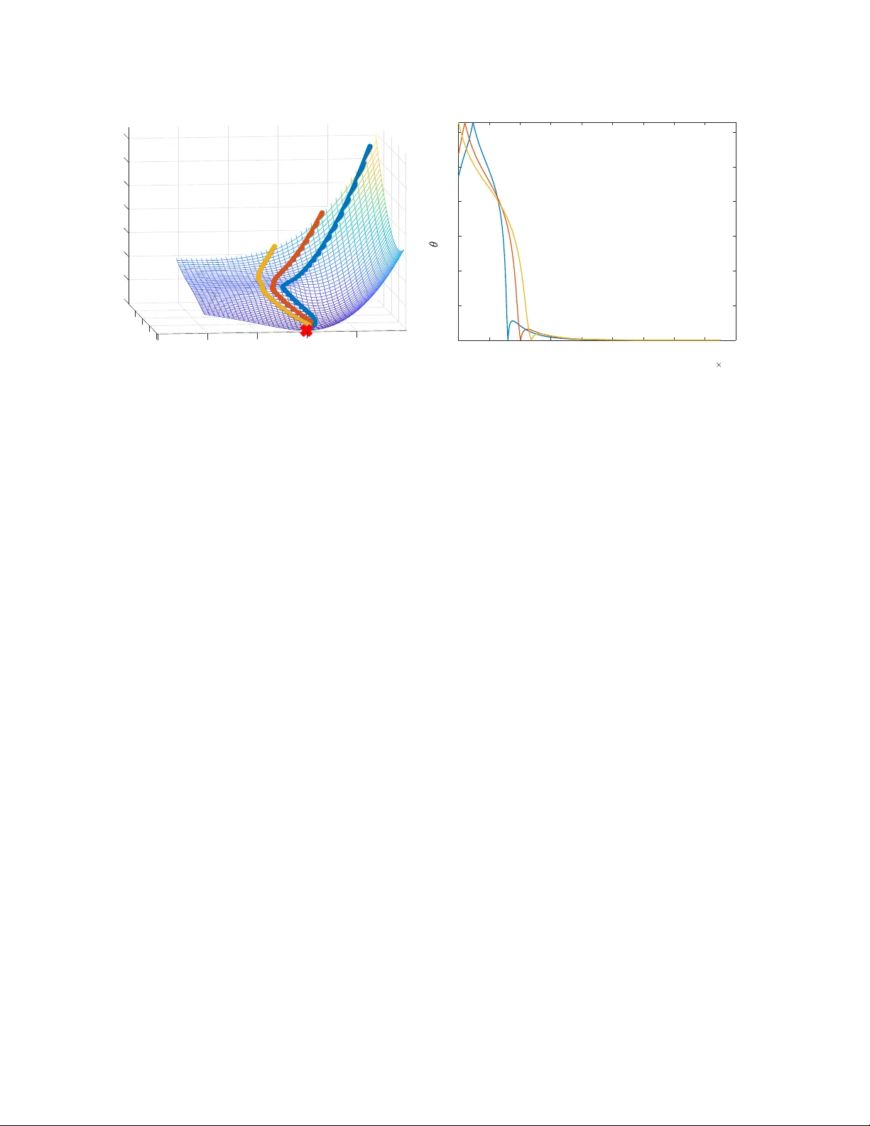
We consider the fundamental problem of learning a single neuron $x \mapsto\sigma(w^\top x)$ using standard gradient methods. As opposed to previous works, which considered specific (and not always realistic) input distributions and activation functio…
Authors: ** 제공되지 않음 (논문에 저자 정보가 명시되지 않았습니다) **
Learning a Single Neuron with Gradient Methods Gilad Y ehudai Ohad Shamir W eizmann Institute of Science { gilad.yehudai,ohad.shamir } @weizmann.ac.il Abstract W e consider the fundamental problem of learning a single neuron x 7→ σ ( w > x ) in a realizable setting, using standard gradient methods with random initialization, and under general families of input distributions and activ ations. On the one hand, we sho w that some assumptions on both the distribution and the activ ation function are necessary . On the other hand, we prove positi ve guarantees under mild assumptions, which go significantly beyond those studied in the literature so far . W e also point out and study the challenges in further strengthening and generalizing our results. 1 Intr oduction In recent years, much effort has been de v oted to understanding wh y neural netw orks are successfully trained with simple, gradient-based methods, despite the inherent non-con ve xity of the learning problem. Howe ver , our understanding of this is still partial at best. In this paper , we focus on the simplest possible nonlinear neural netw ork, composed of a single neuron, of the form x 7→ σ ( w > x ) , where w is the parameter vector and σ : R → R is some fix ed non-linear acti vation function. Moreover , we consider a realizable setting, where the inputs are sampled from some distribution D , the tar get values are generated by some unknown tar get neuron x 7→ σ ( v > x ) (possibly corrupted by independent zero-mean noise, and where we generally assume k v k = 1 for simplicity), and we wish to train our neuron with respect to the squared loss. Mathematically , this boils do wn to minimizing the follo wing objectiv e function: F ( w ) := E x ∼D 1 2 σ ( w > x ) − σ ( v > x ) 2 . (1) For this problem, we are interested in the performance of gradient-based methods, which are the w orkhorse of modern machine learning systems. These methods initialize w randomly , and proceed by taking (gener- ally stochastic) gradient steps w .r .t. F . If we hope to explain the success of such methods on complicated neural networks, it seems reasonable to expect a satisfying e xplanation for their con ver gence on single neu- rons. Although the learning of single neurons was studied in a number of papers (see the related work section belo w for more details), the existing analyses all suffer from one or se veral limitations: Either the y apply for a specific distribution D , which is con venient to analyze b ut not very practical (such as a standard Gaussian distribution); Apply to gradient methods only with a specific initialization (rather than a standard random one); Require technical conditions on the input distribution which are not generally easy to verify; Or require smoothness and strict monotonicity conditions on the activ ation function σ ( · ) (which e xcludes, for example, the common ReLU function σ ( z ) = max { 0 , z } ). Ho wev er , a bit of experimentation strongly suggests 1 that none of these restrictions is really necessary for standard gradient methods to succeed on this simple problem. Thus, our understanding of this problem is probably still incomplete. The goal of this paper is to study to what extent the limitations above can be remo ved, with the follo wing contributions: • W e begin by asking whether positiv e results are possible without any explicit assumptions on the distribution D or the acti vation σ ( · ) (other than, say , bounded support for the former and Lipschitz continuity for the latter). Although this seems reasonable at first glance, we sho w in Sec. 3 that unfor- tunately , this is not the case: Even for the ReLU activ ation function, there are bounded distributions D on which gradient descent will fail to optimize Eq. ( 1 ) with probability exponentially close to 1 . Moreov er , e ven for D which is a standard Gaussian, there are Lipschitz acti vation functions on which gradient methods will likely fail. • Motiv ated by the above, we ask whether it is possible to prove positiv e results with mild and transpar- ent assumptions on the distribution and activ ation function, which does not exclude common setups. In Sec. 4 , we prove a ke y technical result, which implies that if the distribution D is sufficiently “spread” and the activ ation function satisfies a weak monotonicity condition (satisfied by ReLU and all standard activ ation functions), then h∇ F ( w ) , w − v i is positi ve in most of the domain. This im- plies that an exact gradient step with sufficiently small step size will bring us closer to v in “most” places. Building on this result, we prove in Sec. 5 a constant-probability con ver gence guarantee for se veral v ariants of gradient methods (gradient descent, stochastic gradient descent, and gradient flo w) with random initialization. • In Sec. 6 , we consider more specifically the case where D is any spherically symmetric distribution (which includes the standard Gaussian as a special case) and the ReLU activ ation function. In this setting, we show that the con vergence results can be made to hold with high probability , due to the fact that the angle between the parameter vector and the target vector v motonically decreases. As we discuss later on, the case of the ReLU function and a standard Gaussian distribution was also considered in [22, 15], but that analysis crucially relied on initialization at the origin and a Gaussian distribution, whereas our results apply to more generic initialization schemes and distrib utions. • A natural question arising from these results is whether a high-probability result can be proved for non-spherically symmetric distributions. W e study this empirically in Subsection 6.2 , and sho w that perhaps surprisingly , the angle to the tar get function might incr ease rather than decrease, already when we consider unit-variance Gaussian distributions with a non-zero mean. This suggests that a fundamentally dif ferent approach would be required for a general high-probability guarantee. Overall, we hope our w ork contrib utes to a better understanding of the dynamics of gradient methods on simple neural networks, and suggests some natural a venues for future research. 1.1 Related W ork First, we emphasize that learning a single tar get neuron is not an inherently difficult problem: Indeed, it can be efficiently performed with minimal assumptions, using the Isotron algorithm and its variants (Kalai and Sastry [14], Kakade et al. [13]). Also, other algorithms exist for ev en more complicated networks or more general settings, under certain assumptions (e.g., Goel et al. [9], Janzamin et al. [11]). Ho wev er , these are non-standard algorithms, whereas our focus here is on standard, v anilla gradient methods. 2 For this setting, a positiv e result was provided in Mei et al. [16], showing that gradient descent on the empirical risk function 1 n P n i =1 ( σ ( x > i w ) − σ ( x > i v )) 2 (with x i sampled i.i.d. from D and n sufficiently large) successfully yields a good approximation of v . Howe ver , the analysis requires σ to be strictly mono- tonic, and to hav e uniformly bounded deriv ativ es up to the third order . This excludes standard activ ation functions such as the ReLU, which are neither strictly monotonic nor differentiable. Indeed, assuming that the activ ation is strictly monotonic makes the analysis much easier , as we sho w later on in Thm. 3.2 . A related analysis under strict monotonicity conditions is provided in Oymak and Soltanolk otabi [17]. For the specific case of a ReLU activ ation function σ ( · ) = max {· , 0 } and a standard Gaussian input distribution, Tian [26] prov ed that with constant probability , gradient flow ov er Eq. ( 1 ) will asymptotically con ver ge to the global minimum. Soltanolkotabi [22] and Kalan et al. [15] considered a similar setting, and proved a non-asymptotic con vergence guarantee for gradient descent or stochastic gradient descent on the empirical risk function 1 n P n i =1 ( σ ( x > i w ) − σ ( x > i v )) 2 . Ho wev er , that analysis crucially relied on initialization at precisely 0 , as well as a certain assumption on ho w the deri vati ve of the ReLU function is computed at 0 . In more details, we impose the con vention that ev en though the ReLU function is not dif ferentiable at 0 , we take σ 0 (0) to be some fixed positi ve number , and the gradient of the population objecti ve F at 0 to be E x ∼D h ( σ (0) − σ ( v > x )) σ 0 (0) x i = − σ 0 (0) · E x ∼D h σ ( v > x ) x i . Assuming σ 0 (0) > 0 , we get that the gradient is non-zero and proportional to − E x ∼D [ σ ( v > x ) x ] . For a Gaussian distribution (and more generally , spherically symmetric distributions), this turns out to be pro- portional to − v , so that an exact gradient step from 0 will lead us precisely in the direction of the target parameter vector v . As a result, if we calculate a sufficiently precise approximation of this direction from a random sample, we can get arbitrarily close to v in a single iteration (see Kalan et al. [15, Remark 1] for a discussion of this). Unfortunately , this unique beha vior is specific to initialization at 0 with a certain con vention about σ 0 (0) (note that e ven locally around 0 , the gradient may not approximate v , since it is generally discontinuous around 0 ). Thus, although the analysis is important and insightful, it is difficult to apply more generally . Du et al. [6] considered conditions under which a single ReLU con v olutional filter is learnable with gradient methods, a special case of which is a single ReLU neuron. The paper is closely related to our w ork, in the sense that they were also motiv ated by finding general conditions under which positiv e results are attainable. Moreov er , some of the techniques they employed share similarities with ours (e.g., considering the gradient correlation as in Sec. 4 ). Ho we ver , our results differ in sev eral aspects: First, they consider only the ReLU acti vation function, while we also consider general acti vations. Second, their results assume a technical condition on the eigen values of certain distribution-dependent matrices, with the con ver gence rate depending on these eigen values. Howe v er , the question of when might this condition hold (for general distributions) is left unclear . In contrast, our assumptions are more transparent and hav e a clear geometric intuition. Third, their results hold with constant probability , ev en for a standard Gaussian distribution, while we employ a different analysis to pro ve high probability guarantees for general spherically symmetric distributions. Finally , we also provide negati ve results, showing the necessity of assumptions on both the acti vation function and the input distribution, as well as suggesting which approaches might not work for further generalizing our results. A line of recent works established the effecti veness of gradient methods in solving non-conv ex optimiza- tion problems with a strict saddle property , which implies that all near-stationary points with nearly positi ve definite Hessians are close to global minima (see Jin et al. [12], Ge et al. [7], Sun et al. [23]). A relev ant example is phase retriev al, which actually fits our setting with σ ( · ) being the quadratic function z 7→ z 2 (Sun 3 et al. [24]). Ho wev er , these results can only be applied to smooth problems, where the objective function is twice differentiable with Lipschitz-continuous Hessians (excluding, for example, problems inv olving the ReLU activ ation function). An interesting recent exception is the work of T an and V ershynin [25], which considered the case σ ( z ) = | z | . Howe ver , their results are specific to that activ ation, and assumes a specific input distribution D (uniform on a scaled origin-centered sphere). In contrast, our focus here is on more general families of distrib utions and activ ations. Brutzkus and Globerson [3] sho w that gradient descent learns a simple con volutional network with non- ov erlapping patches, when the inputs hav e a standard Gaussian distribution. Similar to the analysis in Sec. 6 in our paper , they rely on showing that the angle between the learned parameter vector and a target vector monotonically decreases with gradient methods. Howe v er , the netw ork architecture studied is dif ferent than ours, and their proof heavily relies on the symmetry of the Gaussian distrib ution. Less directly related to our setting, a popular line of recent works sho wed how gradient methods on highly over -parameterized neural networks can learn various target functions in polynomial time (e.g., Allen- Zhu et al. [1], Daniely [5], Arora et al. [2], Cao and Gu [4]). Howe ver , as pointed out in Y ehudai and Shamir [27], this type of analysis cannot be used to explain learnability of single neurons. 2 Pr eliminaries Notation. W e use bold-faced letters to denote vectors. For a vector w , we let w i denote its i -th coordinate. W e denote [ z ] + := max { 0 , z } to be the ReLU function. For a vector w , we let ¯ w := w k w k , and by 1 1 1 we denote the all-ones vector (1 , . . . , 1) . Gi ven vectors w , v we let θ ( w , v ) := arccos w > v k w kk v k = arccos( ¯ w > ¯ v ) ∈ [0 , π ] denote the angle between w and v . W e use P to denote probability . 1 ( · ) denotes the indicator function, for example 1 ( x > 0) equals 1 if x > 0 and 0 otherwise. T arget Neuron. Unless stated otherwise, we assume that the target vector v in Eq. ( 1 ) is unit norm, k v k = 1 . Gradients. When σ ( · ) is dif ferentiable, the gradient of the objectiv e function in Eq. ( 1 ) is ∇ F ( w ) = E x ∼D h σ ( w > x ) − σ ( v > x ) · σ 0 ( w > x ) x i (2) When σ ( · ) is not differentiable, we will still assume that it is differentiable almost ev erywhere (up to a finite number of points), and that in every point of non-differentiability z , there are well-defined left and right deri vati ves. In that case, practical implementations of gradient methods fix σ 0 ( z ) to be some number between its left and right deriv ati ves (for example, for the ReLU function, σ 0 (0) is defined as some number in [0 , 1] ). Follo wing that con vention, the expected gradient used by these methods still corresponds to Eq. ( 2 ), and we will follo w the same con vention here. Algorithms. In our paper, we focus on the follo wing three standard gradient methods: • Gradient Descent : W e initialize at some w 0 and set a fixed learning rate η . At each iteration t > 0 , we do a single step in the negati ve direction of the gradient: w t +1 = w t − η ∇ F ( w t ) . • Stochastic Gradient Descent (SGD) : W e initialize at some w 0 and set a fixed learning rate η . At each iteration t > 0 , we sample an input x t ∼ D , and calculate a stochastic gradient: g t = σ ( w > t x t ) − σ ( v > x t ) · σ 0 ( w > t x t ) x t (3) 4 and do a single step in the negati ve direction of the stochastic gradient: w t +1 = w t − η g t . Note that here we consider SGD on the population loss, which is dif ferent from SGD on a fixed training set. W e also note that our proof techniques easily extend to mini-batch SGD, where g t is taken to be the av erage of B stochastic gradients w .r .t. x 1 t , . . . , x B t sampled i.i.d. from D . Howe ver , for simplicity we will focus on B = 1 . • Gradient Flow : W e initialize at some w (0) , and for ev ery t > 0 , we set w ( t ) to be the solution of the dif ferential equation: ˙ w ( t ) = −∇ F ( w ( t )) . This can be thought of as a continuous form of gradient descent, where we consider an infinitesimal learning rate. W e note that strictly speaking, gradient flo w is not an algorithm. Howe ver , it approximates the behavior of gradient descent in many cases, and has the adv antage that its analysis is often simpler . 3 Assumptions on the Distribution and Activ ation are Necessary The main concern of this paper is under what assumptions can a single neuron be provably learned with gradient methods. In this section, we show that perhaps surprisingly , this is not possible unless we make non-tri vial assumptions on both the input distribution and the acti vation function. 3.1 Assumptions on the Input Distrib ution ar e Necessary W e begin by asking whether Eq. ( 1 ) can be minimized by gradient methods in a distribution-free manner (with no assumptions beyond, say , bounded support), as in learning problems where the population objective is conv ex. Perhaps surprisingly , we show that the answer is negati ve, e ven if we consider specifically the ReLU acti v ation, and a distrib ution supported on the unit Euclidean ball. This is based on the follo wing k ey result: Theorem 3.1. Suppose that σ is the ReLU function (with the con vention that σ 0 ( z ) = 1 ( z > 0) ), and assume that w is sampled fr om a pr oduct distribution D w (namely , each w i is sampled independently fr om some distrib ution D i w ). Then ther e e xists a distribution D over the inputs, supported on { x : k x k ≤ 1 } , and v with k v k = 1 suc h that the following holds: W ith pr obability at least 1 − exp − d 4 over the initialization point sampled fr om D w , if we run gradient flow , gradient descent or stochastic gradient descent, then for every t > 0 we have F ( w t ) − inf w F ( w ) ≥ 1 8 d (for gradient flow F ( w ( t )) − inf w F ( w ) ≥ 1 8 d ). Pr oof. For each distribution D i w , let p i = P ( w i > 0) . W e define the following dataset: S = { x i = b i e i : i = 1 . . . , d } where e i is the standard i -th unit vector , and b i = 1 if p i < 1 2 and − 1 otherwise. T ake D to be the uniform distribution on S . Informally , the proof idea is the follo wing: W ith overwhelming probability , we will initialize at a point w such that for at least Ω( d ) coordinates i , it holds that σ 0 ( w > x i ) = 0 , and as a result, ∇ F ( w ) is zero on those coordinates. Based on this, we sho w that these coordinates will not change from their initialized v alues. Howe ver , a point w with Ω( d ) coordinates with this property is suboptimal by a fixed factor , so the algorithm does not con ver ge to an optimal solution. More formally , using Eq. ( 2 ) and the fact that σ is the ReLU function, we get ∇ F ( w ) = 1 d d X i =1 σ ( w > x i ) − σ ( v > x i ) · 1 w > x i > 0 x i . 5 In particular , for ev ery index i for which 1 w > x i > 0 = 0 we hav e that ( ∇ F ( w )) i = 0 . Next, we define v with v i = b i 1 √ d (note that k v k = 1 ). For ev ery d/ 4 indices i 1 , . . . , i d/ 4 for which 1 w > x i ≥ 0 = 0 we hav e that: F ( w ) = 1 2 d d X i =1 σ ( w > x i ) − σ ( v > x i ) 2 ≥ 1 2 d X i ∈{ i 1 ,...,i d/ 4 } σ ( w > x i ) − σ ( v > x i ) 2 = 1 2 d X i ∈{ i 1 ,...,i d/ 4 } σ ( v > x i ) 2 = 1 2 d X i ∈{ i 1 ,...,i d/ 4 } σ b 2 i 1 √ d 2 = 1 8 d (4) Denote the random v ariable Z i = 1 w > 0 x i > 0 and Z = P d i =1 Z i (for gradient flow we denote Z i = 1 w (0) > x i ≥ 0 ). It is easily verified that E [ Z i ] = Pr( w > 0 x i > 0) = Pr( w 0 ,i b i > 0) ≤ 1 2 . W e hav e that Z 1 , . . . , Z d are independent, max i | Z i | ≤ 1 , and E [ Z ] = P d i =1 E [ Z i ] ≤ d 2 . Using Hoeffding’ s inequality , we get that w .p ≥ 1 − exp − d 4 it holds that Z ≤ 3 4 d , which means that there are at least d 4 indices such that Z i = 0 . W e condition on this ev ent and let these indices be i 1 , . . . , i d/ 4 . W e will now show that for ev ery index i ∈ { i 1 , . . . , i d/ 4 } , using gradient methods will not change the i -th coordinate of w t ( w ( t ) for gradient flo w) from its initial v alue. Let i be such a coordinate. For gradient descent, we will sho w by induction that for e very iteration t we ha ve that 1 w > t x i > 0 = 0 . The base case is true, because we conditioned on this ev ent. Assume for t − 1 , then ( ∇ F ( w t − 1 )) i = 0 , which means that ( w t ) i = ( w t − 1 ) i − η ( ∇ F ( w t − 1 )) i = ( w t − 1 ) i , and in particular 1 w > t x i > 0 = 1 w > t − 1 x i > 0 = 0 . This proves that for every iteration t , the i -th coordinate of ∇ F ( w t ) is zero, which mean that ( w t ) i = ( w 0 ) i . For stochastic gradient descent, at each iteration t we sample x t ∼ D , and define the stochastic gradient g t as in Eq. ( 3 ). If x t 6 = x i then ( x t ) i = 0 hence ( g t ) i = 0 , otherwise, if x t = x i then by ( g t ) i = ( ∇ F ( w t )) i and by the same induction argument as in gradient descent we hav e that ( g t ) i = 0 . In both cases the i -th coordinate of the stochastic gradient is zero, hence ( w t ) i = ( w 0 ) i . For gradient flow , assume on the way of contradiction that for some t > 0 that 1 w ( t ) > x i > 0 6 = 0 and let t 1 be the first time that this happen. Then for all 0 < t < t 1 we hav e that 1 w ( t ) > x i > 0 = 0 , and in particular ( ∇ F ( w ( t ))) i = 0 . Hence for all 0 < t < t 1 running gradient flow we get ( ˙ w ( t )) i = ( ∇ F ( w ( t ))) i = 0 , and in particular 1 w ( t ) > x i > 0 = 1 w (0) > x i > 0 = 0 , a contradiction to the fact that w ( t ) is continuous. Thus for all t > 0 we showed that 1 w ( t ) > x i > 0 = 0 , hence ( ∇ F ( w ( t ))) i = 0 which sho ws that ( w ( t )) i = ( w (0)) i . By the conditioned ev ent, Eq. ( 4 ) applies at initialization. Since in all the gradient methods above the i -th coordinate of w did not change from its initial value for i ∈ { i 1 , . . . , i d/ 4 } , we can apply Eq. ( 4 ) to get that for every iteration t > 0 for gradient descent or SGD we have that F ( w t ) ≥ 1 8 d (and for gradient flow , for e very time t > 0 , we hav e F ( w ( t )) ≥ 1 8 d ). W e end by noting that although the distribution defined here is discrete ov er a finite dataset, the same argument can also be made for a non-discrete distrib ution, by considering a mixture of smooth distrib utions concentrated around the support points of the discrete distribution abo ve. The theorem abo ve applies to any product initialization scheme, which includes most standard initializa- tions used in practice (e.g., the standard Xavier initialization [8]). The theorem implies that it is impossible to prov e positi ve guarantees in our setting without distrib utional assumptions on ths inputs. Inspecting the construction, the source of the problem (at least for the ReLU neuron) appears to be the fact that the dis- tribution is supported on a small number of well-separated regions. Thus, in our positiv e results, we will assume that the distribution is suf ficiently “spread”, as formalized later on in Sec. 4 6 3.2 Assumptions on the Activation Function W e now turn to discuss the activ ation function, explaining why ev en if the activ ation is Lipschitz and the input distribution D is a standard Gaussian, this is likely insuf ficient for positi ve guarantees in our setting. In particular , let us consider the case that σ ( · ) is a 1 -Lipschitz periodic function. Then Theorem 3 in [21] implies that for a large family of input distributions D on R d (including a standard Gaussian), if we assume that the vector v in the target neuron σ ( v > x ) is a uniformly distributed unit vector , then for any fixed w , V ar v ( ∇ F ( w )) ≤ O (exp( − d )) . This implies that the gradient at w is virtually independent of the underlying target vector v : In fact, it is extremely concentrated around a fix ed v alue which does not depend on v . Theorem 4 from [21] goes further and shows that for any gradient method, even an exponentially small amount of noise will be enough to make its trajectory (after at most exp( O ( d )) iterations) independent of v , in which case it cannot possibly succeed in this setting. W e note that their result is ev en more general as they consider a general function f ( w , x ) instead of σ ( h w , x i ) , so our setting can be seen as a priv ate case. When considering a standard Gaussian distribution, the above argument can be easily extended to ac- ti vations σ which are periodic only in a segment of length Ω( d ) around the origin. This can be seen by extending the activ ation to ˜ σ which is periodic on R , applying the above argument to it, and noting that the probability mass outside of a ball of radius Ω( d ) is exponentially small (for example, see [27] Proposition 4.2, where the y consider an acti vation which is a finite sum of ReLU functions and periodic in a se gment of length O ( d 2 ) ). The above discussion moti vates us to impose some condition on the activ ation function which excludes periodic functions. One such mild assumptions, which we will adopt in the rest of the paper (and corresponds to virtually all activ ations used in practice) is that the activ ation is monotonically non-decreasing. Before continuing, we remark that by assuming a slight strengthening of this assumption, namely that the function is strictly monotonically increasing, it is easy to prove a positi ve guarantee, as evidenced by Thm. 3.2 . Ho wev er , this excludes popular acti vations such as the ReLU function. Theorem 3.2. Assume inf z σ 0 ( z ) ≥ γ > 0 for some γ > 0 , and the following for some λ, c 1 , c 2 : • Σ := E x xx > is positive definite with minimal eigen value λ > 0 • E x ∼D k x k 2 ≤ c 1 • sup z σ 0 ( z ) ≤ c 2 . Then starting fr om any point w 0 , after doing t iterations of gradient descent with learning rate η < λγ 2 c 2 1 c 4 2 , we have that: k w t − v k 2 ≤ k w 0 − v k (1 − λγ 2 η ) t . The proof can be found in Appendix A , and can be easily generalized to apply also to gradient flow and SGD. The above shows that if we assume strict monotonicity of the activ ation, then under very mild assumptions on the data w t will con ver ge e xponentially fast to v . In the rest of the paper , ho wev er , we focus on results which only require weak monotonicity . 7 4 Under Mild Assumptions, the Gradient Points in a Good Direction Moti vated by the results in Sec. 3 , we use the follo wing assumptions on the distribution and acti v ation: Assumption 4.1. The following holds for some fixed α, β , γ > 0 : 1. The distrib ution D satisfies the following: F or any vector w 6 = v , let D w , v denote the mar ginal distri- bution of x on the subspace spanned by w , v (as a distribution over R 2 ). Then any such distribution has a density function p w , v ( x ) suc h that inf x : k x k≤ α p w , v ( x ) ≥ β . 2. σ : R 7→ R is monotonically non-decr easing, and satisfies inf 0 x ) − σ ( v > x ) · σ 0 ( w > x ) · ( w > x − v > x ) i . Note that: 1. Using the assumption on σ , the term inside the above expectation is nonnegati ve for ev ery x . This is because σ 0 ( x ) ≥ 0 , and for an y monotonically non-decreasing function f we hav e ( f ( x ) − f ( y ))( x − y ) ≥ 0 . Thus, vie wing the e xpectation as an inte gral ov er a nonnegati ve function, we can lo wer bound it by taking the integral over the smaller set x ∈ R d : w > x > 0 , v > x > 0 . Note that on this set, σ ( w > x ) = w > x and σ ( v > x ) = v > x . 8 2. The resulting inte gral depends only on dot products of x with w and v . Thus, it is enough to consider the marginal distrib ution on the 2 -dimensional plane spanned by w and v . 3. By the assumption on the distribution, the density function of this marginal distribution is always at least β on any x such that k x k ≤ α . This means we can lower bound the integral above by integrating ov er w with a uniform distribution on this set and multiplying by β . In total, the expression above can be lower bounded by a certain 2 -dimensional integral (with uniform measure and with no σ terms) on the set n y ∈ R 2 : ˆ w > y > 0 , ˆ v > y > 0 , k y k ≤ α o where ˆ w , ˆ v are the 2 -dimensional vectors representing w , v on the 2 -dimensional plane spanned by them. W e lo wer bound this integral by a term that scales with the angle θ ( w , v ) . Remark 4.3 (Implication on Optimization Landscape) . The pr oof of the theor em can be shown to imply that for the ReLU activation, under the theor em’s conditions, the only stationary point that is not the global minimum v must be at the origin. In particular , the pr oof implies that any stationary point (with ∇ F ( w ) = 0 ) must be along the ray { w = − a · v : a ≥ 0 } . F or the ReLU activation (whic h satisfies σ ( z ) σ 0 ( − a · z ) = 0 for any a ≥ 0 and z ), the gradient at such points equals ∇ F ( − a · v ) = E x h ( σ ( − a v > x ) − σ ( v > x )) σ 0 ( − a v > x ) x i = E x h ( − a v > x ) σ 0 ( − a v > x ) x i . In particular , h∇ F ( − a · v ) , v i = − a · E x h σ 0 ( − a v > x )( v > x ) 2 i . This implies that ∇ F ( − a · v ) might be zer o only if either a = 0 (i.e., at the origin), or v > x ≥ 0 with pr obability 1 , which cannot happen accor ding to Assumption 4.1 . 5 Con vergence with Constant Probability Under Mild Assumptions In this section, we use Thm. 4.2 in order to show that under some assumption on the initialization of w , gradient methods will be able to learn a single neuron with probability at least (close to) 1 2 . Note that the loss surface of F ( w ) is not con vex, and as explained in Remark 4.3 , there may be a stationary point at w = 0 . This stationary point can cause difficulties, as it is not obvious ho w to control the angle between v and w close to the origin (which is required for Thm. 4.2 to apply). But, if we assume k w − v k 2 < 1 at initialization, then we are bounded away from the origin, and we can ensure that it will remain that way throughout the optimization process. One such initialization, which guarantees this with at least constant probability , is a zero-mean Gaussian initialization with small enough variance: Lemma 5.1. Assume k v k = 1 . If we sample w ∼ N 0 , τ 2 I for τ ≤ 1 d √ 2 then w .p > 1 2 − 1 4 τ d − 1 . 2 − d we have that k w − v k 2 ≤ 1 − 2 τ 2 d In order to bound each gradient step we will need these additional assumptions: Assumption 5.2. The following holds for some positive c 1 , c 2 : 1. k x k 2 ≤ c 1 almost sur ely over x ∼ D 9 2. σ 0 ( z ) ≤ c 2 for all z ∈ R W ith these assumptions, we show con ver gence for gradient flow , gradient descent and stochastic gradient descent: Theorem 5.3. Under assumptions 4.1 and 5.2 we have: 1. (Gradient Flow) Assume that k w (0) − v k 2 < 1 . Running gradient flow , then for every time t > 0 we have k w ( t ) − v k 2 ≤ k w (0) − v k 2 exp( − tλ ) wher e λ = α 4 β γ 2 210 . 2. (Gradient Descent) Assume that k w 0 − v k 2 < 1 . Let η ≤ λ 2 c for λ = min n 1 , α 4 β γ 2 210 o and c = c 2 1 c 4 2 . Running gradient descent with step size η , we have that for every T > 0 , after T iterations: k w T − v k 2 ≤ k w 0 − v k 2 1 − η λ 2 T 3. (Stochastic Gradient Descent) Let 1 , 2 , δ > 0 , and assume that k w 0 − v k 2 ≤ 1 − 1 . Let η ≤ λ 2 1 2 2 c 2 3 60 c 3 1 c 6 2 log ( 2 δ ) wher e λ = α 4 β γ 2 210 and c 3 = 1 2 λ 20 c 1 c 2 2 − 1 2 λ 18 c 1 c 2 2 . Then w .p 1 − & 20 c 1 c 2 2 log 1 2 λ ' δ , after T ≥ 2 log 1 2 λη iterations we have that: k w T − v k 2 ≤ 2 Combined with Lemma 5.1 , Thm. 5.3 sho ws that with proper initialization, gradient flow , gradient descent as well as stochastic gradient descent successfully minimize Eq. ( 1 ) with probability (close to) 1 2 , and for the first two algorithms, the distance to v decays exponentially f ast. The full proof of the theorem can be found in Appendix C , and its intuition for gradient flow and gradient is as described above (namely , that if k w − v k < 1 , it will stay that way and k w − v k will just continue to shrink over time, using Thm. 4.2 ). The proof for stochastic gradient descent is much more delicate. This is because the update at each iteration is noisy , so we need to ensure we remain in the region where Thm. 4.2 is applicable. Here we give a short proof intuition: 1. Assume we initialized with k w 0 − v k 2 ≤ 1 − for some > 0 . In order for the analysis to work we need that k w t − v k < 1 throughout the algorithm’ s run. Thus, we sho w (using a maximal version of Azuma’ s inequality) that if η is small enough (depending on ), and we take at most m = O 1 η gradient steps then w .h.p for ev ery t = 1 , . . . , m : k w t − v k 2 ≤ 1 − 2 2. The next step is to sho w that if k w t − v k 2 < 1 , then E k w t +1 − v k 2 | w t ≤ (1 − η λ ) k w t − v k 2 for an appropriate λ . This is done using Thm. 4.2 , as in the gradient descent case, but note that here this only holds in expectation o ver the sample selected at iteration t . 3. Next, we use Azuma’ s inequality again on m = O (1 /η ) iterations for a small enough η , to show that w .h.p w m does not move too far away from ˜ w m := E [ w m ] where the expectation is taken ov er x 1 , . . . , x m . Also, we show that after m iterations k ˜ w m − v k 2 ≤ ρ k w 0 − v k 2 for a constant ρ smaller than 1 . This sho ws that w .h.p., after a single epoch of m iterations, k w m − v k shrinks by a constant factor . 10 4. W e then repeat this analysis across t epochs (each consisting of m iterations), and use a union bound. Overall, we get that after sufficiently many iterations, with high probability , the iterates get as close as we want to zero. W e note the optimization analysis for stochastic gradient descent is inspired by the analysis in [20] for the different non-con vex problem of principal component analysis (PCA), which also attempts to av oid a problematic stationary point. An interesting question for future research is to understand to what extent the polynomial dependencies in the problem parameters can be improv ed. Remark 5.4. Our assumption on the data that k x k 2 ≤ c 1 is made for simplicity . F or the gradient descent case, it is easy to verify that the pr oof only r equir es that the fourth moment of the data is bounded by some constant, which ensur es that the gradients of the objective function used by the algorithm ar e bounded. F or SGD it is enough to assume that the input distribution is sub-Gaussian. The pr oof pr oceeds in the same manner , by using a variant of Azuma’ s inequality for martingales with sub-Gaussian tails, e.g . [19]. 6 High-Pr obability Con ver gence The results in the pre vious section hold under mild conditions, but unfortunately only guarantee a constant probability of success. In this section, we consider the possibility of proving guarantees which hold with high probability (arbitrarily close to 1 ). On the one hand, in Subsection 6.1 , we provide such a result for the ReLU activ ation, assuming the input distribution D is spherically symmetric. On the other hand, in Subsection 6.2 , we point out non-trivial obstacles to extending such a result to non-spherically symmetric distributions. Overall, we believ e that getting high-probability conv ergence guarantees for non-spherically symmetric distributions is an interesting a venue for future research. 6.1 Con ver gence for Spherically Symmetric Distributions In this subsection, we make the follo wing assumptions: Assumption 6.1. Assume that: 1. x ∼ D has a spherically symmetric distribution. That is, for every orthogonal matrix A : A x ∼ D 2. The activation function σ ( · ) is the standar d ReLU function σ ( z ) = max { 0 , z } . These assumptions are significantly stronger than Assumptions 4.1 , but allow us to prove a stronger high- probability conv ergence result. Note that even with these assumptions the loss surface is still not con vex, and may contain a spurious stationary point (see Remark 4.3 ). For simplicity , we will focus on proving the result for gradient flow . The result can then be extended to gradient descent and stochastic gradient descent, along similar lines as in the proof of Thm. 5.3 . The proof strategy in this case is quite dif ferent from that of the constant-probability guarantee, and relies on the follo wing key technical result: Lemma 6.2. If w ( t ) 6 = 0 , then ∂ ∂ t θ ( w ( t ) , v ) ≤ 0 The lemma (which relies on the spherical symmetry of the distribution) implies that if we initialize at any point w (0) / ∈ span { v } , then the angle between w (0) and v is strictly less than π , and will remain so as long as w ( t ) 6 = 0 . As a result, we can apply Thm. 4.2 to prove that k w ( t ) − v k decays exponentially fast. The only potential difficulty is that w ( t ) may con ver ge to the potential stationary point at the origin (at which the angle is not well-defined), but fortunately this cannot happen due to the follo wing lemma: 11 Lemma 6.3. Let θ = θ ( w ( t ) , v ) and assume that w ( t ) 6 = 0 . If k w ( t ) k ≤ max n sin( θ )+cos( θ ) 2 , sin( θ )(1+cos( θ )) 2 o then ∂ ∂ t k w ( t ) k 2 ≥ 0 The lemma can be sho wn to imply that as long as θ remains bounded away from π , then k w ( t ) k 2 cannot decrease below some positive number (as its deriv ativ e is positiv e close enough to zero, and k w ( t ) k 2 is a continuous function of t ). The proof idea of both lemmas is based on a technical calculation, where we project the spherically symmetric distribution on the 2 -dimensional subspace spanned by w and v . Using the lemmas abov e, we can get the following con vergence guarantee: Theorem 6.4. Assume we initialize w (0) such that 0 < k w (0) k ≤ 2 , θ ( w (0) , v ) ≤ π − for some > 0 and that Assumption 4.1 (1) holds. Then running gradient flow , we have for all t ≥ 0 k w ( t ) − v k 2 ≤ k w (0) − v k exp( − λt ) wher e λ = α 4 β 8 √ 2 sin 3 8 . W e now note that the assumption of the theorem holds with exponentially high probability under stan- dard initialization schemes. For example, if we use a Gaussian initialization w (0) ∼ N (0 , 1 d I ) , then by standard concentration of measure arguments, it holds w .p > 1 − e − Ω( d ) that θ ( w (0) , v ) is at most (say) 3 π 4 , and w .p > 1 − e − Ω( d ) that k w (0) k ≤ 2 . As a result, by Thm. 6.4 , w .p > 1 − e − Ω( d ) ov er the initialization we hav e k w ( t ) − v k 2 ≤ k w (0) − v k 2 e − Ω( t ) for all t . The full proof of the theorem can be found in Appendix D . Remark 6.5. If we further assume that the distribution is a standar d Gaussian, then it is possible to pr ove Lemma 6.2 and Lemma 6.3 in a much easier fashion. The r eason is that spe cifically for a standar d Gaussian distribution ther e is a closed-form e xpr ession (without the expectation) for the loss and the gradient, see [3], [18]. W e pr ovide the r elevant versions of the lemmas, as well as their pr oofs, in Subsection D.1 . 6.2 Non-monotonic Angle Beha vior The results in the previous subsection crucially relied on the fact that at almost any point w , the angle θ ( w , v ) decreases. This type of analysis was also utilized in works on related settings (e.g., Brutzkus and Globerson [3]). Based on this, it might be tempting to conjecture that this monotonically decreasing angle property (and as a result, high-probability guarantees) can be shown to hold more generally , not just for symmetrically spherical distributions. Perhaps surprisingly , we sho w empirically that this may not be the case, already when we discuss the simple setting of unit v ariance Gaussian with a non-zer o mean. W e emphasize that this does not necessarily mean that gradient methods will not succeed, only that an analysis based on showing monotonic behavior of the rele v ant geometric quantity will not work in general. In particular, in Figure 1 we report the result of running gradient descent (with constant step size η = 10 − 3 ) on our objective function F in R 2 , where the input distribution D is a unit-variance Gaus- sian with mean at (0 , 1) , and our tar get vector is v = (1 , 0) . W e initialize at three different locations: w 1 = ( − 1 1) , w 2 = ( − 1 , 0 . 5) , w 3 = ( − 1 , 0) . Although the algorithm ev entually reaches the global min- imum w = v , the angle between them is clearly non-monotonic, and actually is initially increasing rather than decreasing. Even worse, the angle appears to attain every value in (0 , π ] , so it appears that any analysis using angle-based “safe regions” is bound to f ail. Overall, we conclude that proving a high-probability con ver gence guarantee for gradient methods ap- pears to be an interesting open problem, already in the case of unit-v ariance, non-zero-mean Gaussian input distributions. W e lea ve tackling this problem to future work. 12 0 0.2 0.4 0.6 0.8 1 1.2 1.4 -0.5 0 w 1 0.5 0.5 0 w 2 -0.5 1 -1 -1.5 0 1 2 3 4 5 6 7 8 9 iteration 10 4 0 0.5 1 1.5 2 2.5 3 (w,v) Figure 1: Gradient descent for 2 -dimensional data (best vie wed in color). The left figure represents the trajectory of gradient descent over the loss surface. The red ”x” marker represents the global minimum at w = v = (1 , 0) . The right figure shows the angle between w and v as a function of the number of iterations, where the angle ranges from 0 to π . The plot colors in the right figure correspond to the trajectory colors in the left figure. Acknowledgements. This research is supported in part by European Research Council (ERC) grant 754705. W e thank Itay Safran for spotting a bug in the proof of Thm. 4.2 . Refer ences [1] Z. Allen-Zhu, Y . Li, and Y . Liang. Learning and generalization in ov erparameterized neural networks, going beyond tw o layers. In Advances in Neural Information Pr ocessing Systems , 2019. [2] S. Arora, S. S. Du, W . Hu, Z. Li, and R. W ang. Fine-grained analysis of optimization and generalization for ov erparameterized two-layer neural networks. arXiv pr eprint arXiv:1901.08584 , 2019. [3] A. Brutzkus and A. Globerson. Globally optimal gradient descent for a con vnet with gaussian inputs. In Pr oceedings of the 34th International Confer ence on Machine Learning-V olume 70 . JMLR. org, 2017. [4] Y . Cao and Q. Gu. A generalization theory of gradient descent for learning over -parameterized deep ReLU networks. arXiv pr eprint arXiv:1902.01384 , 2019. [5] A. Daniely . SGD learns the conjugate kernel class of the network. In Advances in Neural Information Pr ocessing Systems , pages 2422–2430, 2017. [6] S. S. Du, J. D. Lee, and Y . Tian. When is a con volutional filter easy to learn? arXiv pr eprint arXiv:1709.06129 , 2017. [7] R. Ge, F . Huang, C. Jin, and Y . Y uan. Escaping from saddle points—online stochastic gradient for tensor decomposition. In Confer ence on Learning Theory , pages 797–842, 2015. 13 [8] X. Glorot and Y . Bengio. Understanding the difficulty of training deep feedforward neural networks. In Pr oceedings of the thirteenth international confer ence on artificial intelligence and statistics , pages 249–256, 2010. [9] S. Goel, V . Kanade, A. Kli vans, and J. Thaler . Reliably learning the relu in polynomial time. arXiv pr eprint arXiv:1611.10258 , 2016. [10] W . Hoef fding. Probability inequalities for sums of bounded random v ariables. In The Collected W orks of W assily Hoeffding , pages 409–426. Springer , 1994. [11] M. Janzamin, H. Sedghi, and A. Anandkumar . Beating the perils of non-con vexity: Guaranteed training of neural networks using tensor methods. arXiv pr eprint arXiv:1506.08473 , 2015. [12] C. Jin, R. Ge, P . Netrapalli, S. M. Kakade, and M. I. Jordan. How to escape saddle points efficiently . In Pr oceedings of the 34th International Confer ence on Machine Learning-V olume 70 , pages 1724–1732. JMLR. org, 2017. [13] S. M. Kakade, V . Kanade, O. Shamir , and A. Kalai. Efficient learning of generalized linear and single index models with isotonic regression. In Advances in Neural Information Pr ocessing Systems , pages 927–935, 2011. [14] A. T . Kalai and R. Sastry . The isotron algorithm: High-dimensional isotonic regression. In COLT . Citeseer , 2009. [15] S. M. M. Kalan, M. Soltanolkotabi, and A. S. A vestimehr . Fitting relus via sgd and quantized sgd. In 2019 IEEE International Symposium on Information Theory (ISIT) , pages 2469–2473. IEEE, 2019. [16] S. Mei, Y . Bai, and A. Montanari. The landscape of empirical risk for non-con ve x losses. arXiv pr eprint arXiv:1607.06534 , 2016. [17] S. Oymak and M. Soltanolkotabi. Overparameterized nonlinear learning: Gradient descent takes the shortest path? arXiv preprint , 2018. [18] I. Safran and O. Shamir . Spurious local minima are common in two-layer relu neural netw orks. arXiv pr eprint arXiv:1712.08968 , 2017. [19] O. Shamir . A v ariant of azuma’ s inequality for martingales with subgaussian tails. arXiv pr eprint arXiv:1110.2392 , 2011. [20] O. Shamir . A stochastic pca and svd algorithm with an exponential con vergence rate. In International Confer ence on Machine Learning , pages 144–152, 2015. [21] O. Shamir . Distribution-specific hardness of learning neural networks. The J ournal of Machine Learn- ing Resear ch , 19(1):1135–1163, 2018. [22] M. Soltanolk otabi. Learning relus via gradient descent. In Advances in Neur al Information Pr ocessing Systems , pages 2007–2017, 2017. [23] J. Sun, Q. Qu, and J. Wright. When are nonconv ex problems not scary? arXiv pr eprint arXiv:1510.06096 , 2015. 14 [24] J. Sun, Q. Qu, and J. Wright. A geometric analysis of phase retrie val. F oundations of Computational Mathematics , 18(5):1131–1198, 2018. [25] Y . S. T an and R. V ershynin. Online stochastic gradient descent with arbitrary initialization solves non-smooth, non-con ve x phase retriev al. arXiv preprint , 2019. [26] Y . Tian. An analytical formula of population gradient for two-layered relu network and its applications in con ver gence and critical point analysis. In Pr oceedings of the 34th International Confer ence on Machine Learning-V olume 70 , pages 3404–3413. JMLR. or g, 2017. [27] G. Y ehudai and O. Shamir . On the power and limitations of random features for understanding neural networks. In Advances in Neural Information Pr ocessing Systems , 2019. A Pr oofs from Sec. 3 Pr oof of Thm. 3.2 . W e hav e that: h∇ F ( w ) , w − v i = E x h ( σ ( w > x ) − σ ( v > x )) σ 0 ( w > x )( w > x − v > x ) i ( ∗ ) = E x h γ · ( σ ( w > x ) − σ ( v > x ))( w > x − v > x ) i ( ∗∗ ) = E x h γ 2 ( w > x − v > x ) 2 i = γ 2 ( w − v ) > Σ( w − v ) ≥ γ 2 λ k w − v k 2 where ( ∗ ) is by monotonicity of σ (hence ( σ ( w > x ) − σ ( v > x ))( w > x − v > x ) ≥ 0 alw ays), and ( ∗∗ ) is by the assumption that σ 0 ( z ) ≥ γ . Next, we bound the gradient ∇ F ( w ) : k∇ F ( w t ) k 2 = E x σ ( w > t x ) − σ ( v > x ) 2 · σ 0 ( w > x ) 2 x > x ≤ c 4 2 E x w > t x − v > x 2 · x > x ≤ c 4 2 k w t − v k 2 E x h k x k 2 · x > x i ≤ c 2 1 c 4 2 k w t − v k 2 . At iteration t + 1 we ha ve that: k w t +1 − v k 2 = k w t − η ∇ F ( w t ) − v k 2 = k w t − v k 2 − 2 η h∇ F ( w t ) , w t − v i + η 2 k∇ F ( w t ) k 2 ≤ k w t − v k 2 − 2 γ 2 λη k w t − v k 2 + η 2 c 2 1 c 4 2 k w t − v k 2 ≤ k w t − v k 2 1 − γ 2 λη . Using induction ov er the above pro ves the lemma. 15 B Pr oofs from Sec. 4 W e will first need the follo wing lemma: Lemma B.1. F ix some α ≥ 0 , and let a , b be two vectors in R 2 such that θ ( a , b ) ≤ π − δ for some δ ∈ (0 , π ] . Then inf u : k u k =1 Z 1 a > y > 0 1 b > y > 0 1 k y k≤ α ( u > y ) 2 d y ≥ α 4 8 √ 2 sin 3 δ 4 . Pr oof. It is enough to lower bound inf u inf b : θ ( a , b ) ≤ π − δ Z 1 a > y > 0 , b > y > 0 , k y k≤ α ( ¯ u > y ) 2 d y . The inner infimum is attained at some b such that θ ( a , b ) = π − δ . This is because ¯ u > y does not depend on a and b , and the volume for which the indicator function inside the integral is non-zero is smallest when the angle θ ( a , b ) is lar gest. Setting this and switching the order of the infima, we get inf b : θ ( a , b )= − π + δ inf u Z 1 a > y > 0 1 b > y > 0 1 k y k≤ α ( ¯ u > y ) 2 d y . When θ ( a , b ) = − π + δ , we note that the set { y ∈ R 2 : a > y > 0 , b > y > 0 , k y k ≤ α } is simply a “pie slice” of radial width δ out of a ball of radius α . Since the e xpression is in v ariant to rotating the coordinates, we will consider without loss of generality the set P = { y : θ ( y , e 1 ) ≤ δ / 2 , k y k ≤ α } , and the expression abov e reduces to inf u Z y ∈ P ( ¯ u > y ) 2 d y = inf u : k u k =1 Z y ∈ P ( u 1 y 1 ) 2 + ( u 2 y 2 ) 2 + 2 u 1 u 2 y 1 y 2 d y ( ∗ ) = inf u : k u k =1 Z y ∈ P ( u 1 y 1 ) 2 + ( u 2 y 2 ) 2 d y = inf u 1 ,u 2 : u 2 1 + u 2 2 =1 u 2 1 Z y ∈ P y 2 1 d y + u 2 2 Z y ∈ P y 2 2 d y = min Z y ∈ P y 2 1 d y , Z y ∈ P y 2 2 d y ≥ Z y ∈ P min { y 2 1 , y 2 2 } d y , (5) where ( ∗ ) is from the fact that P is symmetric around the x -axis (namely , ( y 1 , y 2 ) ∈ P if and only if ( y 1 , − y 2 ) ∈ P ). W e no w note that the set P contains the two (disjoint and equally-sized) rectangular sets P 0 1 := α 2 cos δ 4 , α cos δ 4 × α 2 sin δ 4 , α sin δ 4 and P 0 2 := α 2 cos δ 4 , α cos δ 4 × − α sin δ 4 , − α 2 sin δ 4 16 -0.2 0 0.2 0.4 0.6 0.8 1 1.2 -0.6 -0.4 -0.2 0 0.2 0.4 0.6 /4 /4 P ' 1 P ' 2 Figure 2: An illustration of the sets P , P 0 1 , P 0 2 for the case of α = 1 , δ = π 2 . The set P , colored in gray , is a ”pie slice” and the rectangles P 0 1 , P 0 2 are contained in P . (see Figure 2 for an illustration). Therefore, we can lower bound Eq. ( 5 ) by Z y ∈ P 0 1 ∪ P 0 2 min { y 2 1 , y 2 2 } d y = min y ∈ P 0 1 ∪ P 0 2 min { y 2 1 , y 2 2 } Z y ∈ P 0 1 ∪ P 0 2 1 d y = α 2 4 min cos 2 δ 4 , sin 2 δ 4 · Z y ∈ P 0 1 ∪ P 0 2 1 d y = α 2 4 sin 2 δ 4 · Z y ∈ P 0 1 ∪ P 0 2 1 d y , where we used the fact that δ 4 ∈ 0 , π 4 and therefore cos 2 ( δ / 4) ≥ sin 2 ( δ / 4) . The integral is simply the volume of P 0 1 ∪ P 0 2 , and since P 0 1 and P 0 2 are disjoint and equally sized rectanges, this equals twice the volume of P 0 1 , namely 2 · α 2 cos δ 4 · α 2 sin δ 4 . Plugging into the above, we get α 2 4 sin 2 δ 4 · α 2 2 cos δ 4 sin δ 4 = α 4 8 sin 3 δ 4 cos δ 4 ≥ α 4 8 √ 2 sin 3 δ 4 , where again we used the fact that δ/ 4 ∈ [0 , π / 4] . W e no w turn to prov e the theorem: Pr oof of Thm. 4.2 . W e hav e: h∇ F ( w ) , w − v i = E x h σ ( w > x ) − σ ( v > x ) · σ 0 ( w > x ) · ( w > x − v > x ) i . (6) 17 Let P be the orthogonal projection on the plane spanned by w and v . W e note that since σ is mono- tonically non-decreasing, then for any x , σ 0 ( w > x ) ≥ 0 and ( σ ( w > x ) − σ ( v > ))( w > x − v > x ) ≥ 0 . As a result, we can lo wer bound Eq. ( 6 ) by E x h 1 w > x > 0 1 v > x > 0 σ ( w > x ) − σ ( v > x ) · σ 0 ( w > x ) · ( w > x − v > x ) i ≥ E x h 1 k P x k≤ α 1 w > x > 0 1 v > x > 0 σ ( w > x ) − σ ( v > x ) · γ · ( w > x − v > x ) i = γ · E x h 1 k P x k≤ α 1 w > x > 0 1 v > x > 0 σ ( w > x ) − σ ( v > x ) ( w > x − v > x ) i , where we used that k w k ≤ 2 , hence for k x k ≤ α (and also for k P x k ≤ α , since P is an orthogonal projection) we have h x , w i ≤ 2 α which by our assumption means that σ 0 ( h w , x i ) > γ . By the assumption that σ 0 ( z ) ≥ γ for any 0 < z < 2 α , it follows that ( σ ( z 0 ) − σ ( z )) · ( z 0 − z ) ≥ γ ( z 0 − z ) 2 for any 0 < z , z 0 < 2 α As a result, the displayed equation above is at least γ 2 · E x h 1 k P x k≤ α 1 w > > 0 1 v > x > 0 ( w > x − v > x ) 2 i = γ 2 k w − v k 2 · E x h 1 k P x k≤ α 1 w > x > 0 1 v > x > 0 (( w − v ) > x ) 2 i ≥ γ 2 k w − v k 2 · inf u ∈ span { w , v } , k u k =1 E x h 1 k P x k≤ α 1 w > x > 0 1 v > x > 0 ( u > x ) 2 i Since the expression inside the expectation above depends just on inner products of x with w , v , we can consider the marginal distrib ution D w , v of x on the 2 -dimensional subspace spanned by w , v (with density function p w , v ), and letting ˆ w , ˆ v denote the projections of w , v on that subspace, write the abov e as γ 2 k w − v k 2 · inf u ∈ R 2 , k u k =1 E y ∼D w , v h 1 ˆ w > y > 0 1 ˆ v > y > 0 1 k y k≤ α ( u > y ) 2 i = γ 2 k w − v k 2 · inf u ∈ R 2 , k u k =1 Z 1 ˆ w > y > 0 1 ˆ v > y > 0 1 k y k≤ α ( u > y ) 2 p w , v ( y ) d y ≥ β γ 2 k w − v k 2 · inf u ∈ R 2 , k u k =1 Z 1 ˆ w > y > 0 1 ˆ v > y > 0 1 k y k≤ α ( u > y ) 2 d y , where the last step is by our assumptions (note that if w = v , the theorem statement is trivially true by Eq. ( 6 ) which implies that the inner product is non-negati ve). The theorem no w follows from Lemma B.1 . C Pr oofs from Sec. 5 Pr oof of Lemma 5.1 . Fix some > 0 to be determined later . W e have that: P k w − v k 2 ≤ 1 − = P k w k 2 − 2 h w , v i ≤ − = P h w , v i ≥ k w k 2 + 2 . Since the distrib ution of w is spherically symmetric, we can assume w .l.o.g that v = (1 , 0) , so that h w , v i = w 1 . Thus, the above probability can be written as: P h w , v i ≥ k w k 2 + 2 = P w 1 ≥ k w k 2 + 2 ≥ P w 1 ≥ 2 E k w k 2 − P k w k 2 + 2 ≥ 2 E k w k 2 (7) 18 where we used the fact that for ev ery two random v ariable A, B and constant c we ha ve that P ( A ≥ B ) ≥ P ( A ≥ c ) − P ( B ≥ c ) . For the first term of Eq. ( 7 ), we kno w that E k w k 2 = τ 2 d , hence: P w 1 ≥ 2 E k w k 2 = P w 1 ≥ 2 τ 2 d = 1 2 − 1 2 erf √ 2 τ d where erf is the error function. For any 0 < z < 1 it can be easily verified that erf ( z ) ≥ z 3 . Combining this and using the assumption that τ ≤ 1 d √ 2 we can bound : P w 1 ≥ 2 E k w k 2 ≥ 1 2 − 1 3 √ 2 τ d ≥ 1 2 − 1 4 τ d For the second term of Eq. ( 7 ) tak e = 2 τ 2 d to get: P k w k 2 + 2 ≥ 2 E k w k 2 = P k w k 2 ≥ 4 τ 2 d − ≤ P k w k 2 ≥ 2 τ 2 d ≤ 2 e − 1 d/ 2 ≤ 1 . 2 − d where in the second inequality we used a standard tail bound on Chi-squared distributions. Combining the abov e with Eq. ( 7 ) we get that: P k w − v k 2 ≤ 1 − 2 τ 2 d ≥ 1 2 − 1 4 τ d − 1 . 2 − d . C.1 Gradient Flow Pr oof of Thm. 5.3 (1). First we show that at ev ery time t 0 for which k w ( t 0 ) − v k < 1 the conditions of Thm. 4.2 hold. W e have that k w ( t 0 ) k ≤ k w ( t 0 ) − v k + k v k < 2 , hence k w ( t 0 ) k < 2 . Next k w ( t 0 ) − v k 2 < 1 and k v k 2 = 1 hence h w ( t 0 ) , v i ≥ 1 2 k w ( t 0 ) k 2 > 0 which means that θ ( w ( t 0 ) , v ) < π 2 . This shows that we can use Thm. 4.2 at time t = t 0 to get that: ∂ ∂ t k w ( t ) − v k 2 = 2 h w ( t ) − v , ∂ ∂ t w ( t ) i = − 2 h w ( t ) − v , ∇ F ( w ( t )) i ≤ 0 . (8) By the assumptions of the theorem, the abov e holds for time t 0 = 0 . Assume on the way of contradiction that for some time t > 0 we have that k w ( t ) − v k ≥ 1 , and let t 1 be the first time that this happens. Then for every t 0 < t < t 1 we have that k w ( t ) − v k < 1 . But because k w ( t 1 ) − v k ≥ 1 we have that for some time t 0 < t < t 1 : ∂ ∂ t k w ( t ) − v k > 0 , a contradiction to Eq. ( 8 ). Hence for ev ery t ≥ 0 we have that k w ( t ) − v k < 1 and the conditions of Thm. 4.2 hold. Using Thm. 4.2 again we get that for e very t > 0 : h∇ F ( w ( t )) , w ( t ) − v i ≥ α 4 β γ 2 8 √ 2 sin π 8 3 k w ( t ) − v k 2 ≥ α 4 β γ 2 210 | w ( t ) − v k 2 . Set λ = α 4 β γ 2 210 , in total we hav e that: ∂ ∂ t k w ( t ) − v k 2 = − 2 h∇ F ( w ( t )) , w ( t ) − v i ≤ − λ k w ( t ) − v k 2 . Using Gr ¨ onwall’ s inequality , this proves that for e very t > 0 we get: k w ( t ) − v k 2 ≤ k w (0) − v k 2 exp( − λt ) . 19 C.2 Gradient Descent Pr oof of Thm. 5.3 (2). Assume that k w t − v k 2 < 1 for some t ≥ 0 , then we have that θ ( w t , v ) ≤ π 2 . Thus, we can use Thm. 4.2 with δ = π 2 to get that: k w t +1 − v k 2 = k w t − η ∇ F ( w t ) − v k 2 = k w t − v k 2 − 2 η h∇ F ( w t ) , w t − v i + η 2 k∇ F ( w t ) k 2 ≤ k w t − v k 2 (1 − η λ ) + η 2 k∇ F ( w t ) k 2 . No w to bound the second term of the above e xpression recall the definition of ∇ F ( w t ) to get: k∇ F ( w t ) k 2 = E x σ ( w > t x ) − σ ( v > x ) 2 · σ 0 ( w > x ) 2 x > x ≤ c 4 2 E x w > t x − v > x 2 · x > x ≤ c 4 2 k w t − v k 2 E x h k x k 2 · x > x i ≤ c 2 1 c 4 2 k w t − v k 2 where in the first inequality we used that σ is monotonic with bounded deri v ativ e, and in the second inequal- ity we used Cauchy-Schwartz. Note that by our choice of η : 1 − η λ + η 2 c < 1 − η λ 2 < 1 , this prov es that: k w t +1 − v k 2 ≤ (1 − η λ + η 2 c ) k w t − v k 2 ≤ 1 − η λ 2 k w t − v k 2 (9) and in particular k w t +1 − v k < 1 . Now after T iterations we can use Eq. ( 9 ) iterativ ely to get that: k w T − v k 2 ≤ 1 − η λ 2 k w T − 1 − v k 2 ≤ ... ≤ 1 − η λ 2 T k w 0 − v k 2 . C.3 Stochastic Gradient Descent First, we prove a recursion relation similar to the one in the gradient descent step. Only here since each gradient step is stochastic we can only prove that the recursion relation holds in expectation ov er the example selected in each iteration. Lemma C.1. Suppose that k w t − v k 2 ≤ 1 − . Then E k w t +1 − v k 2 | w t ≤ (1 − 2 η λ + η 2 c ) k w t − v k 2 wher e c = c 2 1 c 4 2 . 20 Pr oof. W e can use Thm. 4.2 with δ = π 2 to get that E k w t +1 − v k 2 | w t = E k w t − η g t − v k 2 | w t = k w t − v k 2 − 2 η E [ h g t , w t − v i| w t ] + η 2 E [ k g t k 2 | w t ] = k w t − v k 2 − 2 η h∇ F ( w t ) , w t − v i + η 2 k∇ F ( w t ) k 2 ≤ k w t − v k 2 (1 − 2 η λ ) + η 2 k∇ F ( w t ) k 2 . No w to bound the second term recall the definition of ∇ F ( w t ) to get: k∇ F ( w t ) k 2 = E x σ ( w > t x ) − σ ( v > x ) 2 · σ 0 ( w > x ) 2 x > x ≤ c 4 2 E x w > t x − v > x 2 · x > x ≤ c 4 2 k w t − v k 2 E x h k x k 2 · x > x i ≤ c 2 1 c 4 2 k w t − v k 2 where in the first inequality we used that σ is monotonic with bounded deri v ativ e, and in the second inequal- ity we used Cauchy-Schwartz. This prov es the required bound. The recursion relation abov e only works if w t is in a ”safe zone”, that is k w t − v k 2 ≤ 1 − . Although in e xpectation the distance between w t and v only decrease, taking a stochastic step may tak e w t +1 outside of the safe zone. The follo wing lemma shows that if η is small enough, then taking at most m = O (1 /η ) steps keeps w t in the ”safe zone” w .h.p for ev ery t = 1 , . . . , m . Lemma C.2. Assume that k w 0 − v k 2 ≤ 1 − , and Let δ > 0 . Then w .p > 1 − δ , if η < 2 λ 3 c 2 1 c 4 2 log ( 1 δ ) and m ≤ 1 9 η c 1 c 2 2 then for every i = 1 , . . . , m we have that k w i − v k 2 ≤ 1 − 2 . Pr oof. Denote X i = k w i − v k 2 , then we hav e: | X i − X i − 1 | = k w i − v k 2 − k w i − 1 − v k 2 = k w i − 1 − η g i − 1 − v k 2 − k w i − 1 − v k 2 = − 2 η h g i − 1 , w i − 1 − v i + η 2 k g i − 1 k 2 ≤ 2 η |h g i − 1 , w i − 1 − v i| + η 2 k g i − 1 k 2 (10) W e will bound the norm of the gradient at each step: k g i k 2 = x > i x i σ 0 w > i x i 2 σ w > i x i − σ v > x i 2 ≤ c 2 1 c 4 2 k w i − v k 2 thus we can bound Eq. ( 10 ) with: | X i − X i − 1 | ≤ k w i − 1 − v k 2 c 2 1 c 4 2 (2 η + η 2 ) ≤ 3 η c 2 1 c 4 2 k w i − 1 − v k 2 (11) Denote η 0 = 3 η c 2 1 c 4 2 . Using Eq. ( 10 ) we can bound: k w i − v k 2 ≤ k w i − 1 − v k 2 + η 0 k w i − 1 − v k 2 ≤ (1 + η 0 ) k w i − 1 − v k 2 (12) Thus, combining Eq. ( 11 ) and Eq. ( 12 ) we get: | X i − X i − 1 | ≤ η 0 (1 + η 0 ) k w i − 2 − v k 2 ≤ ... ≤ η 0 (1 + η 0 ) i − 2 k w 0 − v k 2 ≤ η 0 (1 + η 0 ) i (1 − ) 21 W e would like to use Azuma’ s inequality on X i , but in order to prove that they are supermartingales we need to use Lemma C.1 . The problem here is that the condition of the lemma, that k w t − v k 2 < 1 − , does not necessarily holds, hence the series X i may not be supermartingales. Instead, we consider a dual series of random v ariables ˜ X i = min X i , 1 − 2 , and prov e that they are supermartingales. First we hav e that: ˜ X i − ˜ X i − 1 ≤ | X i − X i − 1 | ≤ η 0 (1 + η 0 ) i (1 − ) . Next, we hav e for ev ery i that ˜ X i ≤ 1 − 2 , thus we can use Lemma C.1 (note that the result of the lemma does not depend on the v alue of ) and choose η 0 ≤ λ c 2 1 c 4 2 to get that: E [ ˜ X i | w i − 1 ] ≤ min { (1 − 2 η 0 λ + η 0 2 c 2 1 c 4 2 ) X i − 1 , 1 − } ≤ ˜ X i − 1 this prov es that the series ˜ X i are supermartingales. Now we use a maximal version of Azuma-Hoeffding inequality (see [10]) on ˜ X i to sho w that after m iterations we hav e that: P sup 1 ≤ i ≤ m ˜ X i − ˜ X 0 > 2 ≤ exp − 2 2 P m i =0 ( η 0 (1 + η 0 ) i (1 − )) 2 ! ≤ exp − 2 2 η 0 2 (1 − ) 2 (1+ η 0 ) 2 m +2 − 1 (1+ η 0 ) 2 − 1 ≤ exp − 2 2 η 0 2 (1 − ) 2 2 (1+ η 0 ) 2 − 1 ! ≤ exp − 2 (2 + η 0 ) 4 η 0 (1 − ) 2 (13) where in the second to last inequality we used that η 0 ≤ 1 2 m +2 to bound (1 + η 0 ) 2 m +2 < 3 for every m . Substituting the r .h.s of Eq. ( 13 ) with δ and simplifying the term we get that if η 0 ≤ 2 log ( 1 δ ) then w .p > 1 − δ , for e very i = 1 , . . . , m (note that ˜ X 0 = X 0 ): min n X i , 1 − 2 o ≤ X 0 − 2 ≤ 1 − + 2 = 1 − 2 . In particular , the abov e shows that w .p > 1 − δ for ev ery i = 1 , . . . , m : X i = k w i − v k 2 ≤ 1 − 2 . Next we show that taking a single epoch of m = O (1 /η ) iterations w .h.p will decrease the distance between w and v by a constant that does not depend on the epoch length or the step size. Lemma C.3. Let δ > 0 , tak e η ≤ λ 2 1 2 2 c 2 3 60 c 3 1 c 6 2 log ( 2 δ ) wher e c 3 = 1 2 λ 20 c 1 c 2 2 − 1 2 λ 18 c 1 c 2 2 , and m = 1 9 η c 1 c 2 2 . Assume 2 ≤ k w 0 − v k 2 ≤ 1 − 1 . Then w .p 1 − δ we have that k w m − v k 2 ≤ 1 2 λ 20 c 1 c 2 2 k w 0 − v k 2 . Pr oof. Denote ˜ w i = E [ w i ] where the expectation is ov er x 1 , . . . , x i , and let Z i = k w i − ˜ w i k 2 , then we hav e that: | Z i − Z i − 1 | = k w i − ˜ w i k 2 − k w i − 1 − ˜ w i − 1 k 2 = k w i − 1 − η g i − 1 − ˜ w i − 1 + η ∇ F ( ˜ w i − 1 ) k 2 − k w i − 1 − ˜ w i − 1 k 2 ≤ 2 η |h∇ F ( ˜ w i − 1 ) − g i − 1 , w i − 1 − ˜ w i − 1 i| + η 2 k F ( ˜ w i − 1 ) − g i − 1 k 2 ≤ 2 η k F ( ˜ w i − 1 ) − g i − 1 k · k w i − 1 − ˜ w i − 1 k + η 2 k F ( ˜ w i − 1 ) − g i − 1 k 2 ≤ 2 η ( k∇ F ( ˜ w i − 1 ) k + k g i − 1 k ) · ( k w i − 1 k + k ˜ w i − 1 k ) + η k∇ F ( ˜ w i − 1 ) k 2 + k g i − 1 k 2 (14) 22 As in the proof of the pre vious lemma we can bound: k g i k 2 ≤ c 1 c 2 2 k w i − v k 2 ≤ c 2 1 c 4 2 where we used our assumption that k w i − v k 2 ≤ 1 . In the same manner we can bound k∇ F ( ˜ w i ) k ≤ c 2 1 c 4 2 . Again using our assumption we ha ve that: k w i k ≤ k v k + k w i − v k ≤ 1 + 1 − ≤ 2 and in the same manner k ˜ w i k ≤ 2 . In total we can bound Eq. ( 14 ) by: | Z i − Z i − 1 | ≤ 16 η c 2 1 c 4 2 Set c 3 = 1 2 λ 20 c 1 c 2 2 − 1 2 λ 18 c 1 c 2 2 , we no w us Azuma’ s inequality and Z 0 = 0 to get that: P ( Z m ≥ 2 c 3 ) ≤ exp − 2 2 c 2 3 256 mη 2 c 4 1 c 8 2 Substituting the r .h.s with δ 2 we hav e that for : m ≤ 2 2 c 2 3 512 c 4 1 c 8 2 η 2 log 2 δ (15) then w .p > 1 − δ 2 : k w m − ˜ w m k 2 ≤ 2 c 3 . T ake m = 1 9 η c 1 c 2 2 , by taking η ≤ λ 2 1 2 2 c 2 3 60 c 3 1 c 6 2 log ( 2 δ ) we hav e that Eq. ( 15 ) is satisfied and 1 − η λ + η 2 c ≤ 1 − η λ 2 . Finally , using Lemma C.2 with δ 2 and using a union bound, we get that after m iterations w .p > 1 − δ : k w m − v k 2 ≤ k ˜ w m − v k 2 + k w m − ˜ w m k 2 ≤ 1 − η λ + η 2 c m k w 0 − v k 2 + 2 c 3 ≤ 1 − η λ 2 m k w 0 − v k 2 + 1 2 λ 20 c 1 c 2 2 − 1 2 λ 18 c 1 c 2 2 ! k w 0 − v k 2 ≤ 1 − η λ 2 2 λη ! λ 18 c 1 c 2 2 k w 0 − v k 2 + 1 2 λ 20 c 1 c 2 2 − 1 2 λ 18 c 1 c 2 2 ! k w 0 − v k 2 ≤ 1 2 λ 18 c 1 c 2 2 k w 0 − v k 2 + 1 2 λ 20 c 1 c 2 2 − 1 2 λ 18 c 1 c 2 2 ! k w 0 − v k 2 ≤ 1 2 λ 20 c 1 c 2 2 k w 0 − v k 2 where in the second to last inequality we used that (1 + x ) 1 x ≤ 1 2 for 0 ≤ x ≤ 1 . No w we are ready to prove the main theorem, by taking enough epochs with m iterations, and applying union bound: 23 Pr oof of Thm. 5.3 (3). W e use Lemma C.3 to get that after m = 1 9 η c 1 c 2 2 iterations we hav e w .p 1 − δ k w m − v k 2 ≤ 1 2 λ 20 c 1 c 2 2 k w 0 − v k 2 . Using the abov e iterati vely for t epochs and applying union bound, we ha ve that after T = t · m iterations w .p 1 − tδ : k w t · m − v k 2 ≤ 1 2 tλ 20 c 1 c 2 2 k w 0 − v k 2 ≤ 1 2 tλ 20 c 1 c 2 2 . Setting t = & 20 c 1 c 2 2 log 1 2 λ ' we have w .p > 1 − & 20 c 1 c 2 2 log 1 2 λ ' δ , after T = t · m = 2 log 1 2 λη iterations we hav e: k w T − v k 2 ≤ 1 2 tλ 20 c 1 c 2 2 ≤ 2 D Pr oofs from Sec. 6 In the proofs of this section, we follo w the con vention that for the ReLU function σ ( · ) , it holds that σ 0 ( z ) = 1 ( z ≥ 0) (and in particular, that σ 0 (0) = 1 ). Howe ver , the same proofs will hold assuming any other value of σ 0 (0) in [0 , 1] . Pr oof of Lemma 6.2 . Using the chain rule and the lemma assumption that k w ( t ) k > 0 (hence the angle expression is well-defined), we ha ve ∂ ∂ t θ ( w ( t ) , v ) = ∂ ∂ t arccos w ( t ) > ¯ v k w ( t ) k = − 1 r 1 − w ( t ) > ¯ v k w ( t ) k 2 · k w ( t ) k ¯ v − ( w ( t ) > ¯ v ) w ( t ) k w ( t ) k k w ( t ) k 2 > ( −∇ F ( w ( t ))) = 1 q 1 − ( ¯ w ( t ) > ¯ v ) 2 · ¯ v − ( ¯ w ( t ) > ¯ v ) ¯ w ( t ) k w ( t ) k > ∇ F ( w ( t )) . Thus, it is enough to sho w that: v − ( ¯ w ( t ) > v ) k w ( t ) k w ( t ) > ∇ F ( w ( t )) ≤ 0 . W e fix w = w ( t ) , and denote a = ¯ w > v k w k . Plugging in the definition of ∇ F ( w ) , we want to sho w that E x h σ ( w > x ) − σ ( v > x ) · σ 0 ( w > x ) · ( v > x − a w > x ) i ≤ 0 . 24 Using the assumption that σ is ReLU, the abov e can be rewritten as E x h σ ( w > x ) − σ ( v > x ) · ( v > x − a w > x ) · 1 ( w > x ≥ 0) i ≤ 0 . (16) W e no w note that the expression abov e depends only on inner products of x with w , v , so we can rewrite the inequality as E y ∼D w , v h σ ( ˆ w > y ) − σ ( ˆ v > y ) · ( ˆ v > y − a ˆ w > y ) · 1 ( ˆ w > y ≥ 0) i ≤ 0 , where D w , v is the marginal distribution of x on the 2-dimensional subspace span { w , v } , and ˆ w , ˆ v ∈ R 2 are the representations of w , v in that subspace. Moreov er , by the spherical symmetry of the distribution, the expression above is in variant to rotating the coordinate frame, so we can assume without loss of generality that ˆ w = k w k 1 0 , in which case the abov e reduces to E y ∼D w , v " k w k 1 0 > y − σ ( ˆ v > y ) ! · ˆ v > y − h ¯ w , v i 1 0 > y ! · 1 ( y 1 > 0) # ≤ 0 . Denote g ( y ) = k w k 1 0 > y − σ ( ˆ v > y ) ! · ˆ v > y − h ¯ w , v i 1 0 > y ! , so that the inequality above is E y ∼D w , v [ g ( y ) · 1 ( y 1 > 0)] ≤ 0 . (17) The function g ( y ) can be simplified as: g ( y ) = ( k w k y 1 − σ ( y 1 ˆ v 1 + y 2 ˆ v 2 )) · ( y 1 ˆ v 1 + y 2 ˆ v 2 − ˆ v 1 y 1 ) = ( k w k y 1 − σ ( y 1 ˆ v 1 + y 2 ˆ v 2 )) · y 2 ˆ v 2 , where we used the fact that h ¯ w , v i = h 1 k w k ˆ w , ˆ v i = v 1 . W e no w perform a case analysis to justify Eq. ( 17 ), depending on the value of a (which by definition, equals ¯ w > v k w k = w > v k w k 2 = ˆ w > ˆ v k w k 2 = ˆ v 1 k w k ). In all the cases we assume y 1 > 0 , otherwise the expression in the expectation is zero. • 0 ≤ a ≤ 1 : In this case ˆ v 1 ≥ 0 , and also h ¯ w , v i ≤ k w k . Assume w .l.o.g that ˆ v 2 ≥ 0 (the other case is similar), and for y = y 1 y 2 denote ˜ y = y 1 − y 2 . If y 2 < 0 then g ( y ) ≤ 0 , on the other hand if y 2 > 0 then we can re write: g ( y ) = y 2 ˆ v 2 · ( y 1 ( k w k − ˆ v 1 ) − y 2 ˆ v 2 ) = y 2 ˆ v 2 · ( y 1 ( k w k − h ¯ w , v i ) − y 2 ˆ v 2 ) , where we hav e two cases: 1. if y 1 ( k w k − h ¯ w , v i ) > y 2 ˆ v 2 then | g ( ˜ y ) | ≥ g ( y ) and also g ( ˜ y ) ≤ 0 2. If y 1 ( k w k − h ¯ w , v i ) ≤ y 2 ˆ v 2 then g ( y ) ≤ 0 . W e sho wed that for ev ery y ∈ R 2 either g ( y ) ≤ 0 or there is a unique ˜ y ∈ R 2 with the same norm as y such that g ( ˜ y ) ≤ 0 and | g ( ˜ y ) | ≥ g ( y ) . Since D has a spherical symmetric distribution this shows that Eq. ( 17 ) holds for these v alues of a . 25 • a ≤ 0 : In this case ˆ v 1 ≤ 0 , we also assume w .l.o.g that ˆ v 2 ≥ 0 (the other case is similar). Here for e very y with y 2 ≤ 0 we ha ve that: g ( y ) = ( k w k y 1 − σ ( y 1 ˆ v 1 + y 2 ˆ v 2 )) · y 2 ˆ v 2 = k w k y 1 · y 2 ˆ v 2 ≤ 0 , because y 1 ≥ 0 . On the other hand, if y 2 ≥ 0 we ha ve two cases: 1. If also ˆ v 1 y 1 + ˆ v 2 y 2 ≤ 0 then g ( y ) = k w k y 1 · y 2 ˆ v 2 ≥ 0 , and then g ( ˜ y ) = − g ( y ) . 2. If ˆ v 1 y 1 + ˆ v 2 y 2 ≥ 0 then g ( y ) = ( k w k y 1 − ˆ v 1 y 1 − ˆ v 2 y 2 ) · y 2 ˆ v 2 . If g ( y ) ≥ 0 , then g ( ˜ y ) ≤ 0 and also | g ( ˜ y ) | ≥ g ( y ) . Hence we prov ed that for every y with y 1 > 0 either g ( y ) ≤ 0 or there is ˜ y with | g ( ˜ y ) | ≥ g ( y ) and g ( ˜ y ) ≤ 0 . Since D has a spherical symmetric distribution this shows that Eq. ( 17 ) holds for these v alues of a . • a ≥ 1 : In this case ˆ v 1 ≥ 0 and h ˆ w , v i ≥ k w k . Assume w .l.o.g that ˆ v 2 ≥ 0 (the other case is similar). If y 2 > 0 then g ( y ) = ( y 1 ( k w k − ˆ v 1 ) − y 2 ˆ v 2 ) · y 2 ˆ v 2 ≤ 0 . If y 2 < 0 then we ha ve two case: 1. y 1 ˆ v 1 + y 2 ˆ v 2 ≤ 0 , then g ( y ) = k w k y 1 · y 2 ˆ v 2 < 0 2. y 1 ˆ v 2 + y 2 ˆ v 2 > 0 , in which case if g ( y ) > 0 then g ( ˜ y ) < 0 and g ( ˜ y ) ≥ g ( y ) . Hence for ev ery y with y 1 > 0 either g ( y ) < 0 or there is ˜ y with g ( ˜ y ) < 0 and g ( ˜ y ) ≥ g ( y ) . This sho ws that Eq. ( 17 ) holds for these values of a . Pr oof of Lemma 6.3 . By our assumption w ( t ) 6 = 0 , hence the gradient of the objectiv e is well-defined and we hav e that ∂ ∂ t k w ( t ) k 2 = − w ( t ) > ∇ F ( w ( t )) = E x h σ ( v > x ) − σ ( w ( t ) > x ) σ 0 ( w ( t ) > x ) w ( t ) > x i . (18) Fix w = w ( t ) . Using the assumption that σ is the ReLU function we can rewrite Eq. ( 18 ) as: E x h σ ( v > x ) − w > x · w > x · 1 ( w > x ≥ 0) i . (19) Since the function inside the expectation in Eq. ( 19 ) depends only on the inner product of x with w and v , we can consider the mar ginal distrib ution D w , v on the 2-dimensional subspace span { w , v } , we also denote ˆ w , ˆ v ∈ R 2 as the representations of w , v on this 2-dimensional subspace. W e can now re write Eq. ( 19 ) as: E y ∼D w , v h σ ( ˆ v > y ) − ˆ w > y · ˆ w > y · 1 ( ˆ w > y ≥ 0) i . (20) Note that the function inside the expectation in Eq. ( 20 ) is homogeneous with respect to the norm of y . Also, by our assumption D is a spherically symmetric distribution, hence also D w , v is spherically symmetric. Thus, in order to prove that Eq. ( 20 ) is non-negati ve, it is enough to consider the conditional distribution D w , y , 1 of y on the set { y : k y k = 1 } . Since D w , v , 1 (as a distribution on R 2 ) is still spherically symmetric, 26 it is in v ariant to a rotation of the coordinate system, so we can assume w .l.o.g that ˆ w = k w k 1 0 . Overall, in order to prov e that Eq. ( 20 ) is non-negati ve it is enough to sho w that: E y ∼D w , v , 1 [( σ ( ˆ v 1 y 1 + ˆ v 2 y 2 ) − k w k y 1 ) 1 ( y 1 ≥ 0) · y 1 k w k ] ≥ 0 . (21) Since D is spherically symmetrical and the function inside Eq. ( 21 ), the marginal distribution D w , v , 1 is actually a uniform distribution on { y ∈ R 2 : k y k = 1 } . Thus, in order to sho w that Eq. ( 21 ) is non-negati ve, we can di vide it by k w k (which is positi ve), and sho w that the follo wing integral is non-neg ativ e: Z 1 0 σ v 1 y 1 + v 2 q 1 − y 2 1 − k w k y 1 y 1 + σ v 1 y 1 − v 2 q 1 − y 2 1 − k w k y 1 y 1 dy 1 = Z 1 0 y 1 σ v 1 y 1 + v 2 q 1 − y 2 1 + σ v 1 y 1 − v 2 q 1 − y 2 1 − 2 k w k y 2 1 dy 1 , where we wrote y 2 = ± p 1 − y 2 1 since k y k = 1 . W e can assume w .l.o.g that v 2 ≥ 0 (the other direction is similar) and write v 2 = p 1 − v 2 1 , and thus it is enough to prov e that: Z 1 0 y 1 σ v 1 y 1 + q (1 − y 2 1 )(1 − v 2 1 ) − 2 k w k y 2 1 dy 1 ≥ 0 . (22) Denote θ = θ ( w , v ) , since h ¯ w , v i = h ˆ ¯ w , ˆ v i = v 1 then v 1 = cos( θ ) and p 1 − v 2 1 = sin( θ ) . Now we split into cases for the dif ferent values of v 1 : • v 1 ≥ 0 : In this case, if 0 ≤ y 1 ≤ 1 then v 1 y 1 + p (1 − y 2 1 )(1 − v 2 1 ) ≥ 0 , hence the inte gral in Eq. ( 22 ) can be calculated as: Z 1 0 y 1 v 1 y 1 + q (1 − y 2 1 )(1 − v 2 1 ) − 2 k w k y 2 1 dy 1 = v 1 3 + p 1 − v 2 1 3 − 2 k w k 3 . (23) Thus, the abov e term is non-negati ve if: k w k ≤ v 1 + p 1 − v 2 1 2 = sin( θ ) + cos( θ ) 2 . • v 1 ≤ 0 : In this case, if 0 ≤ y 1 ≤ p 1 − v 2 1 then v 1 y 1 + p (1 − y 2 1 )(1 − v 2 1 ) ≥ 0 , and if p 1 − v 2 1 < y 1 ≤ 1 then v 1 y 1 + p (1 − y 2 1 )(1 − v 2 1 ) ≤ 0 . Thus, the integral in Eq. ( 22 ) can be calculated as: Z √ 1 − v 2 1 0 y 1 v 1 y 1 + q (1 − y 2 1 )(1 − v 2 1 ) − 2 k w k y 2 1 dy 1 − Z 1 √ 1 − v 2 1 2 k w k y 2 1 dy 1 = − 2 k w k 3 + v 3 1 p 1 − v 2 1 3 + v 1 p 1 − v 2 1 3 3 + p 1 − v 2 1 3 = − 2 k w k 3 + p 1 − v 2 1 (1 + v 1 ) 3 . Thus, the abov e term is non-negati ve if: k w k ≤ p 1 − v 2 1 (1 + v 1 ) 2 = sin( θ )(1 + cos( θ )) 2 27 Pr oof of Thm. 6.4 . Assume we initialized with θ ( w (0) , v ) ≤ π − and 0 < k w (0) k ≤ 2 . First we will sho w that w ( t ) 6 = 0 for all t > 0 . Assume on the way of contradiction that for some t > 0 we hav e w ( t ) = 0 , and let t 1 be the first time for which it happens. For t 0 = 0 we know that w ( t 0 ) 6 = 0 , and also that for all t ∈ [ t 0 , t 1 ] , w ( t ) 6 = 0 and the gradient of the objecti ve is well defined. Hence by Lemma 6.2 we know that θ ( w ( t ) , v ) ≤ π − for all t ∈ [ t 0 , t 1 ] , because the angle can only decrease unless w ( t ) = 0 . But, by Lemma 6.3 we know that if k w ( t ) k ≤ max n sin( ) − cos( ) 2 , sin( )(1 − cos( )) 2 o then ∂ ∂ t k w ( t ) k ≥ 0 . In particular , for ∈ (0 , π ] and for all t 0 ≤ t < t 1 , we ha ve that k w ( t ) k is bounded belo w by max n sin( ) − cos( ) 2 , sin( )(1 − cos( )) 2 o > 0 , a contradiction to w ( t 1 ) = 0 . This shows that for all t > 0 we hav e that w ( t ) 6 = 0 , hence by Lemma 6.2 we know that for e very t > 0 we will ha ve θ ( w ( t ) , v ) ≤ π − . No w we can use Thm. 4.2 (where γ = 1 because of Assumption 6.1 (3)) to get: h∇ F ( w ( t )) , w ( t ) − v i ≥ α 4 β 8 √ 2 sin 8 3 k w ( t ) − v k 2 . Set λ = α 4 β 8 √ 2 sin 8 3 , as explained above for all t > 0 , ∇ F ( w ( t )) is continuous since w ( t ) 6 = 0 and we hav e that: ∂ ∂ t k w ( t ) − v k 2 = 2 h w ( t ) − v , ∂ ∂ t w ( t ) i = − 2 h w ( t ) − v , ∇ F ( w ( t )) i ≤ − λ k w ( t ) − v k 2 , Using Gr ¨ onwall’ s inequality , this proves that for e very t > 0 we get: k w ( t ) − v k 2 ≤ k w (0) − v k 2 exp( − λt ) . D.1 Standard Gaussian Distribution In this subsection we assume that D = N (0 , I ) , and that σ is the ReLU function. Lemma D .1. If w ( t ) 6 = 0 , then ∂ ∂ t θ ( w ( t ) , v ) ≤ 0 Pr oof. Similar to the proof of Lemma 6.2 , it is enough to prove that ¯ v − ( ¯ w ( t ) > ¯ v ) ¯ w ( t ) > ∇ F ( w ( t )) ≤ 0 , (24) where we used that k w ( t ) k > 0 hence the angle e xpression is differentiable. In the standard Gaussian case, ∇ F ( w ( t )) has a closed-form e xpression (see [3], [18]), namely ∇ F ( w ) = 1 2 w − 1 2 π ( k v k sin( θ ( w , v )) ¯ w + ( π − θ ( w , v ) v )) . (25) Multiplying this by ¯ v − ( ¯ w ( t ) > ¯ v ) ¯ w ( t ) , and noting that this vector is orthogonal to w ( t ) (as it is simply 28 the component of ¯ v orthogonal to ¯ w ( t ) , we get that ¯ v − ( ¯ w ( t ) > ¯ v ) ¯ w ( t ) > ∇ F ( w ( t )) = ¯ v − ( ¯ w ( t ) > ¯ v ) ¯ w ( t ) > − π − θ ( w ( t ) , v ) 2 π v = − π − θ ( w ( t ) , v ) 2 π ¯ v > v − ( ¯ w ( t ) > ¯ v )( ¯ w ( t ) > v ) = − π − θ ( w ( t ) , v ) 2 π k v k − k v k ( ¯ w ( t ) > ¯ v ) 2 = − π − θ ( w ( t ) , v ) 2 π 1 − ( ¯ w ( t ) > ¯ v ) 2 k v k . Since θ ( w ( t ) , v ) ∈ [ − π , π ] and ¯ w ( t ) > ¯ v ∈ [ − 1 , 1] , it follo ws that this expression is non-negati ve, establish- ing Eq. ( 24 ) and hence the lemma. Lemma D.2. Let θ ( w ( t ) , v ) = π − α and assume that w ( t ) 6 = 0 . If k w ( t ) k ≤ k v k π 4 α 3 , then ∂ ∂ t k w ( t ) k 2 ≥ 0 Pr oof. Using the closed-form expression for ∇ F ( w ) (see Eq. ( 25 )), we ha ve ∂ ∂ t k w ( t ) k 2 = w ( t ) > ∂ ∂ t w ( t ) = − w ( t ) > ∇ F ( w ( t )) = − k w ( t ) k 2 2 + 1 2 π k v kk w ( t ) k sin( θ ( w ( t ) , v )) + ( π − θ ( w ( t ) , v ) w ( t ) > v ) = k w ( t ) kk v k 2 π sin( θ ( w ( t ) , v )) + ( π − θ ( w ( t ) , v )) ¯ w ( t ) > ¯ v − π k w ( t ) k k v k = k w ( t ) kk v k 2 sin( θ ( w ( t ) , v )) + ( π − θ ( w ( t ) , v )) cos( θ ( w ( t ) , v )) − π k w ( t ) k k v k The expression sin( θ ) + ( π − θ ) cos( θ ) can be easily verified to be strictly monotonically decreasing in θ ∈ (0 , π ) , and equal 0 at θ = π . Therefore, if θ ≤ π − α , then the expression abov e can be lower bounded by k w ( t ) kk v k 2 sin( π − α ) + α cos( π − α ) − π k w ( t ) k k v k = k w ( t ) kk v k 2 sin( α ) − α cos( α ) − π k w ( t ) k k v k . (26) T o slightly simplify this expression, we will no w ar gue that sin( α ) − α cos( α ) ≥ α π 3 ∀ α ∈ [0 , π ] . (27) Assuming this inequality holds, we get that Eq. ( 26 ) is at least k w ( t ) kk v k 2 α π 3 − π k w ( t ) k k v k , which is non-negati ve as long as k w ( t ) k ≤ k v k α 3 /π 4 , proving the lemma. It only remains to establish Eq. ( 27 ). W e consider two cases: 29 • If α ∈ [0 , π / 2] , then by a T aylor expansion of sin( α ) , cos( α ) around 0 , we ha ve sin( α ) − α cos( α ) ≥ α − α 3 3! − α 1 − α 2 2! + α 4 4! = α 3 1 2! − 1 3! − α 2 4! ≥ α 3 1 2! − 1 3! − ( π / 2) 2 4! which is at least α 3 / 5 . • If α ∈ π 2 , π , it is easily v erified via dif ferentiation that sin( α ) − α cos( α ) ≥ sin( α ) is monotonically increasing in α . Therefore, it can be lo wer bounded by sin( π / 2) − ( π/ 2) cos( π / 2) = 1 ≥ α 3 /π 3 . Combining the two cases, Eq. ( 27 ) follo ws. 30
Original Paper
Loading high-quality paper...
Comments & Academic Discussion
Loading comments...
Leave a Comment