The Microsoft 2016 Conversational Speech Recognition System

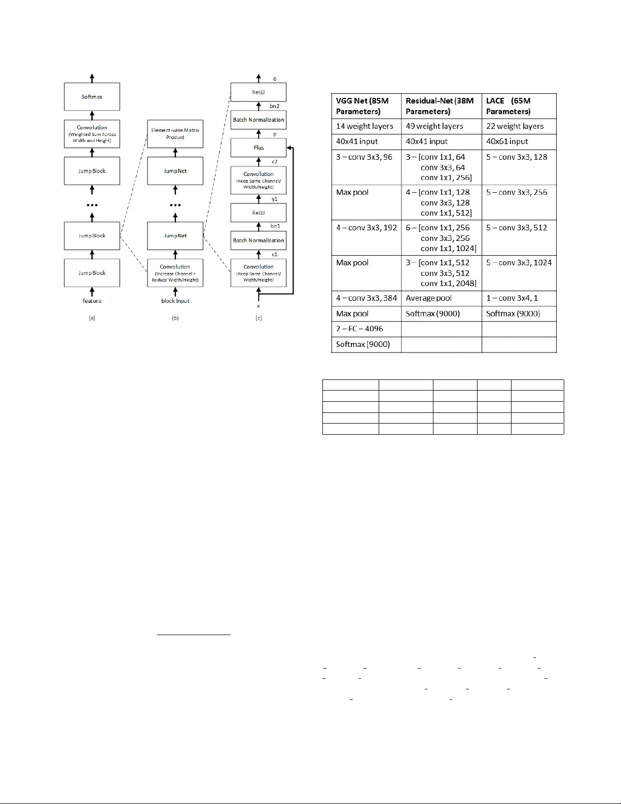
THE MICR OSOFT 2016 CONVERSA TIONAL SPEECH RECOGNITION SYSTEM W . Xiong, J . Dr oppo, X. Huang , F . Seide, M. Seltzer , A. Stolcke , D. Y u and G. Zweig Microsoft Research ABSTRA CT W e describe Microsoft’ s con versational speech recognition system, in which we combine recent dev elopments in neural-network-based acoustic and language modeling to advance the state of the art on the Switchboard recognition task. Inspired by machine learning ensem- ble techniques, the system uses a range of con volutional and recur - rent neural networks. I-vector modeling and lattice-free MMI train- ing provide significant gains for all acoustic model architectures. Language model rescoring with multiple forward and backward run- ning RNNLMs, and word posterior-based system combination pro- vide a 20% boost. The best single system uses a ResNet architecture acoustic model with RNNLM rescoring, and achie ves a word error rate of 6.9% on the NIST 2000 Switchboard task. The combined system has an error rate of 6.2%, representing an improvement o ver previously reported results on this benchmark task. Index T erms — Con versational speech recognition, con volu- tional neural netw orks, recurrent neural networks, VGG, ResNet, LA CE, BLSTM. 1. INTR ODUCTION Recent years ha ve seen a rapid reduction in speech recognition error rates as a result of careful engineering and optimization of con vo- lutional and recurrent neural networks. While the basic structures hav e been well kno wn for a long period [1, 2, 3, 4, 5, 6, 7], it is only recently that they hav e dominated the field as the best models for speech recognition. Surprisingly , this is the case for both acoustic modeling [8, 9, 10, 11, 12, 13] and language modeling [14, 15]. In comparison to standard feed-forw ard MLPs or DNNs, these acoustic models have the ability to model a large amount of acoustic context with temporal in variance, and in the case of con volutional models, with frequency inv ariance as well. In language modeling, recurrent models appear to improve over classical N-gram models through the generalization ability of continuous word representations [16]. In the meantime, ensemble learning has become commonly used in se veral neural models [17, 18, 15], to improv e robustness by reducing bias and variance. In this paper , we use ensembles of models extensiv ely , as well as improvements to individual component models, to to advance the state-of-the-art in conv ersational telephone speech recognition (CTS), which has been a benchmark speech recognition task since the 1990s. The main features of this system are: 1. An ensemble of two fundamental acoustic model architec- tures, conv olutional neural nets (CNNs) and long-short-term memory nets (LSTMs), with multiple variants of each 2. An attention mechanism in the LA CE CNN which differen- tially weights distant context [19] 3. Lattice-free MMI training [20, 21] 4. The use of i-vector based adaptation [22] in all models 5. Language model (LM) rescoring with multiple, recurrent neural net LMs [14] running in both forward and reverse direction 6. Confusion network system combination [23] coupled with search for best system subset, as necessitated by the large number of candidate systems. The remainder of this paper describes our system in detail. Sec- tion 2 describes the CNN and LSTM models. Section 3 describes our implementation of i-vector adaptation. Section 4 presents out lattice-free MMI training process. Language model rescoring is a significant part of our system, and described in Section 5. Experi- mental results are presented in Section 6, followed by a discussion of related work and conclusions. 2. CONV OLUTIONAL AND LSTM NEURAL NETWORKS W e use three CNN variants. The first is the VGG architecture of [24]. Compared to the networks used pre viously in image recognition, this network uses small (3x3) filters, is deeper , and applies up to fi ve con- volutional layers before pooling. The second network is modeled on the ResNet architecture [25], which adds highway connections [26], i.e. a linear transform of each layer’ s input to the layer’ s output [26, 27]. The only difference is that we move the Batch Normaliza- tion node to the place right before each ReLU activ ation. The last CNN variant is the LA CE (layer-wise context expan- sion with attention) model [19]. LA CE is a TDNN [3] variant in which each higher layer is a weighted sum of nonlinear transforma- tions of a windo w of lo wer layer frames. In other w ords, each higher layer exploits broader context than lower layers. Lower layers fo- cus on extracting simple local patterns while higher layers extract complex patterns that co ver broader contexts. Since not all frames in a windo w carry the same importance, an attention mask is ap- plied. The LA CE model dif fers from the earlier TDNN models e.g. [3, 28] in the use of a learned attention mask and ResNet like lin- ear pass-through. As illustrated in detail in Figure 1, the model is composed of 4 blocks, each with the same architecture. Each block starts with a con volution layer with stride 2 which sub-samples the input and increases the number of channels. This layer is followed by 4 RELU-con volution layers with jump links similar to those used in ResNet. T able 1 compares the layer structure and parameters of the three CNN architectures. While our best performing models are con volutional, the use of long short-term memory networks is a close second. W e use a bidirectional architecture [29] without frame-skipping [9]. The core model structure is the LSTM defined in [8]. W e found that using net- works with more than six layers did not improve the word error rate on the development set, and chose 512 hidden units, per direction, per layer, as that provided a reasonable trade-off between training time and final model accurac y . Network parameters for dif ferent configurations of the LSTM architecture are summarized in T able 2. Fig. 1 . LA CE network architecture 3. SPEAKER AD APTIVE MODELING Speaker adapti ve modeling in our system is based on conditioning the network on an i-vector [30] characterization of each speaker [22, 31]. A 100-dimensional i-vector is generated for each con ver - sation side. For the LSTM system, the conv ersation-side i-vector v s is appended to each frame of input. For con volutional netw orks, this approach is inappropriate because we do not expect to see spatially contiguous patterns in the input. Instead, for the CNNs, we add a learnable weight matrix W l to each layer , and add W l v s to the ac- tiv ation of the layer before the nonlinearity . Thus, in the CNN, the i-vector essentially serv es as an additional bias to each layer . Note that the i-v ectors are estimated using MFCC features; by using them subsequently in systems based on log-filterbank features, we may benefit from a form of feature combination. 4. LA TTICE-FREE SEQUENCE TRAINING After standard cross-entrop y training, we optimize the model param- eters using the maximum mutual information (MMI) objecti ve func- tion. Denoting a w ord sequence by w and its corresponding acoustic realization by a , the training criterion is X w,a ∈ data log P ( w ) P ( a | w ) P 0 w P ( w 0 ) P ( a | w 0 ) . As noted in [32, 33], the necessary gradient for use in backpropa- gation is a simple function of the posterior probability of a particu- lar acoustic model state at a given time, as computed by summing ov er all possible word sequences in an unconstrained manner . As first done in [20], and more recently in [21], this can be accom- plished with a straightforward alpha-beta computation ov er the finite state acceptor representing the decoding search space. In [20], the T able 1 . Comparison of CNN architectures T able 2 . Bidirectional LSTM configurations Hidden-size Output-size i-vectors Depth P arameters 512 9000 N 6 43.0M 512 9000 Y 6 43.4M 512 27000 N 6 61.4M 512 27000 Y 6 61.8M search space is taken to be an acceptor representing the composi- tion H C LG for a unigram language model L on words. In [21], a language model on phonemes is used instead. In our implementation, we use a mixed-history acoustic unit lan- guage model. In this model, the probability of transitioning into a new context-dependent phonetic state (senone) is conditioned both the senone and phone history . W e found this model to perform bet- ter than either purely word-based or phone-based models. Based on a set of initial experiments, we de veloped the follo wing procedure: 1. Perform a forced alignment of the training data to select le xi- cal variants and determine frame-aligned senone sequences. 2. Compress consecutiv e frame wise occurrences of a single senone into a single occurrence. 3. Estimate an unsmoothed, variable-length N-gram language model from this data, where the history state consists of the previous phone and pre vious senones within the current phone. T o illustrate this, consider the sample senone sequence { s s2.1288, s s3.1061, s s4.1096 } , { eh s2.527, eh s3.128, eh s4.66 } , { t s2.729, t s3.572, t s4.748 } . When predicting the state following eh s4.66 the history consists of ( s , eh s2.527, eh s3.128, eh s4.66), and fol- lowing t s2.729, the history is ( eh , t s2.729). W e construct the denominator graph from this language model, and HMM transition probabilities as determined by transition- counting in the senone sequences found in the training data. Our approach not only largely reduces the complexity of building up the language model but also provides very reliable training performance. W e hav e found it con venient to do the full computation, without pruning, in a series of matrix-vector operations on the GPU. The un- derlying acceptor is represented with a sparse matrix, and we main- tain a dense likelihood vector for each time frame. The alpha and beta recursions are implemented with CUSP ARSE lev el-2 routines: sparse-matrix, dense vector multiplies. Run time is about 100 times faster than real time. As in [21], we use cross-entropy regularization. In all the lattice-free MMI (LFMMI) experiments mentioned below we use a trigram language model. Most of the gain is usually obtained after processing 24 to 48 hours of data. 5. LM RESCORING AND SYSTEM COMBINA TION An initial decoding is done with a WFST decoder, using the archi- tecture described in [34]. W e use an N-gram language model trained and pruned with the SRILM toolkit [35]. The first-pass LM has approximately 15.9 million bigrams, tri- grams, and 4grams, and a vocabulary of 30,500 words. It gives a perplexity of 69 on the 1997 CTS ev aluation transcripts. The initial decoding produces a lattice with the pronunciation variants marked, from which 500-best lists are generated for rescoring purposes. Subsequent N-best rescoring uses an unpruned LM comprising 145 million N-grams. All N-gram LMs were estimated by a maxi- mum entropy criterion as described in [36]. 5.1. RNNLM setup The N-best hypotheses are then rescored using a combination of the large N-gram LM and se veral RNNLMs, trained and evaluated using the CUED-RNNLM toolkit [37]. Our RNNLM configuration has sev eral distinctiv e features, as described below . 1) W e trained both standard, forward-predicting RNNLMs and backward RNNLMs that predict words in re verse temporal order . The log probabilities from both models are added. 2) As is customary , the RNNLM probability estimates are inter- polated at the word-le vel with corresponding N-gram LM probabili- ties (separately for the forward and backward models). In addition, we trained a second RNNLM for each direction, obtained by starting with dif ferent random initial weights. The two RNNLMs and the N- gram LM for each direction are interpolated with weights of (0.375, 0.375, 0.25). 3) In order to make use of LM training data that is not fully matched to the target conv ersational speech domain, we start RNNLM training with the union of in-domain (here, CTS) and out-of-domain (e.g., W eb) data. Upon conv ergence, the network un- dergoes a second training phase using the in-domain data only . Both training phases use in-domain v alidation data to regulate the learning rate schedule and termination. Because the size of the out-of-domain data is a multiple of the in-domain data, a standard training on a sim- ple union of the data would not yield a well-matched model, and hav e poor perplexity in the tar get domain. 4) W e found best results with an RNNLM configuration that had a second, non-recurrent hidden layer . This produced lower perplex- ity and word error than the standard, single-hidden-layer RNNLM architecture [14]. 1 The overall network architecture thus had two hidden layers with 1000 units each, using ReLU nonlinearities. T raining used noise-contrastiv e estimation (NCE) [38]. 1 Howe ver , adding more hidden layers produced no further gains. T able 3 . Performance of various versions of RNNLM rescoring. Perplexities (PPL) are computed on 1997 CTS ev al transcripts; word error rates (WER) on the NIST 2000 Switchboard test set. Language model PPL WER 4-gram LM (baseline) 69.4 8.6 + RNNLM, CTS data only 62.6 7.6 + W eb data training 60.9 7.4 + 2nd hidden layer 59.0 7.4 + 2-RNNLM interpolation 57.2 7.3 + backward RNNLMs - 6.9 5) The RNNLM output vocab ulary consists of all words oc- curring more than once in the in-domain training set. While the RNNLM estimates a probability for unknown words, we take a dif- ferent approach in rescoring: The number of out-of-set words is recorded for each hypothesis and a penalty for them is estimated for them when optimizing the relativ e weights for all model scores (acoustic, LM, pronunciation), using the SRILM nbest-optimize tool. 5.2. T raining data The 4-gram language model for decoding was trained on the avail- able CTS transcripts from the DARP A EARS program: Switchboard (3M words), BBN Switchboard-2 transcripts (850k), Fisher (21M), English CallHome (200k), and the University of W ashington con- versational W eb corpus (191M). A separate model was trained from each source and interpolated with weights optimized on R T -03 tran- scripts. For the unpruned large rescoring 4-gram, an additional LM component was added, trained on 133M word of LDC Broadcast News te xts. The N-gram LM configuration is modeled after that de- scribed in [31], except that max ent smoothing was used. The RNNLMs were trained on Switchboard and Fisher tran- scripts as in-domain data (20M words for gradient computation, 3M for validation). T o this we added 62M words of UW W eb data as out-of-domain data, for use in the two-phase training procedure de- scribed abov e. 5.3. RNNLM perf ormance T able 3 gives perplexity and word error performance for various RNNLM setups, from simple to more complex. The acoustic model used was the ResNet CNN. As can be seen, each of the measures described earlier adds in- cremental gains, which, while small indi vidually , add up to a 9% relativ e error reduction ov er a plain RNNLM. 5.4. System Combination The LM rescoring is carried out separately for each acoustic model. The rescored N-best lists from each subsystem are then aligned into a single confusion network [23] using the SRILM nbest-ro ver tool. Howe ver , the number of potential candidate systems is too large to allow an all-out combination, both for practical reasons and due to ov erfitting issues. Instead, we perform a greedy search, starting with the single best system, and successively adding additional systems, to find a small set of systems that are maximally complementary . The R T -02 Switchboard set was used for this search procedure. The relativ e weighting (for confusion-network mediated v oting) of the different systems is optimized using an EM algorithm, using the same data, and smoothed hierarchically by interpolating each set of system weights with the preceding one in the search. 6. EXPERIMENT AL SETUP AND RESUL TS 6.1. Speech corpora W e train with the commonly used English CTS (Switchboard and Fisher) corpora. Evaluation is carried out on the NIST 2000 CTS test set, which comprises both Switchboard (SWB) and CallHome (CH) subsets. The Switchboard-1 portion of the NIST 2002 CTS test set was used for tuning and de velopment. The acoustic training data is comprised by LDC corpora 97S62, 2004S13, 2005S13, 2004S11 and 2004S09; see [20] for a full description. 6.2. 1-bit SGD T raining All presented models are costly to train. T o make training feasi- ble, we parallelize training with our previously proposed 1-bit SGD parallelization technique [39]. This data-parallel method distributes minibatches ov er multiple worker nodes, and then aggreg ates the sub-gradients. While the necessary communication time would oth- erwise be prohibiti ve, the 1-bit SGD method eliminates the bottle- neck by two techniques: 1-bit quantization of gradients and auto- matic minibatch-size scaling . In [39], we showed that gradient values can be quantized to just a single bit, if one carries over the quantization error from one mini- batch to the next. Each time a sub-gradient is quantized, the quanti- zation error is computed and remembered, and then added to the next minibatch’ s sub-gradient. This reduces the required bandwidth 32- fold with minimal loss in accuracy . Secondly , automatic minibatch- size scaling progressi vely decreases the frequency of model updates. At regular interv als (e.g. ev ery 72h of training data), the trainer tries larger minibatch sizes on a small subset of data and picks the largest that maintains training loss. 6.3. Acoustic Model Details Forty-dimensional log-filterbank features were extracted e very 10 milliseconds, using a 25-millisecond analysis windo w . The CNN models used windo w sizes as indicated in T able 1, and the LSTMs processed one frame of input at a time. The b ulk of our models use three state left-to-right triphone models with 9000 tied states. Additionally , we hav e trained several models with 27k tied states. The phonetic in ventory includes special models for noise, vocalized- noise, laughter and silence. W e use a 30k-vocab ulary derived from the most common words in the Switchboard and Fisher corpora. The decoder uses a statically compiled unigram graph, and dynamically applies the language model score. The unigram graph has about 300k states and 500k arcs. All acoustic models were trained using the open-source Computational Network T oolkit (CNTK) [40]. T able 4 shows the result of i-vector adaptation and LFMMI train- ing on sev eral of our systems. W e achiev e a 5–8% relativ e improve- ment from i-vectors, including on CNN systems. The last row of T able 4 shows the effect of LFMMI training on the different models. W e see a consistent 7–10% further relativ e reduction in error rate for all models. Considering the great increase in procedural simplicity of LFMMI over the previous practice of writing lattices and post- processing them, we consider LFMMI to be a significant advance in technology . 6.4. Comparative System Perf ormance Model performance for our individual models as well as relev ant comparisons from the literature are shown in T able 5. Out of the 15 models built, only models giv en non-zero weight in the final system combination are shown. T able 4 . Performance improv ements from i-vector and LFMMI training on the NIST 2000 CTS set Configuration WER (%) ReLU-DNN BLSTM LA CE CH SWB CH SWB CH SWB Baseline 21.9 13.4 17.3 10.3 16.9 10.4 i-vector 20.1 11.5 17.6 9.9 16.4 9.3 i-vector+LFMMI 17.9 10.2 16.3 8.9 15.2 8.5 T able 5 . W ord error rates (%) on the NIST 2000 CTS test set with different acoustic models (unless otherwise noted, models are trained on the full 2000 hours of data and hav e 9k senones) Model N-gram LM Neural LM CH SWB CH SWB Saon et al. [31] LSTM 15.1 9.0 - - Pov ey et al. [21] LSTM 15.3 8.5 - - Saon et al. [31] Combination 13.7 7.6 12.2 6.6 300h ResNet 19.2 10.0 17.7 8.2 ResNet GMM alignment 15.3 8.8 13.7 7.3 ResNet 14.8 8.6 13.2 6.9 VGG 15.7 9.1 14.1 7.6 LA CE 14.8 8.3 13.5 7.1 BLSTM 16.7 9.0 15.3 7.8 27k Senone BLSTM 16.2 8.7 14.6 7.5 Combination 13.3 7.4 12.0 6.2 7. RELA TION TO PRIOR WORK Compared to earlier applications of CNNs to speech recognition [41, 42], our networks are much deeper , and use linear bypass con- nections across conv olutional layers. They are similar in spirit to those studied more recently by [11, 10, 31, 12, 13]. W e improve on these architectures with the LA CE model [19], which iterativ ely expands the effecti ve windo w size, layer-by-layer , and adds an at- tention mask to dif ferentially weight distant conte xt. Our use of lattice-free MMI is distincti ve, and extends previous w ork [20, 21] by proposing the use of a mixed triphone/phoneme history in the language model. On the language modeling side, we achieve a performance boost by combining multiple RNNLMs in both forward and backward di- rections, and by using a two-phase training regimen to get best re- sults from out-of-domain data. For our best CNN system, RNNLM rescoring yields a relati ve word error reduction of 20%, and a 16% relativ e gain for the combined recognition system. (Elsewhere we report further improv ements, using LSTM-based LMs [43].) 8. CONCLUSIONS W e have described Microsoft’ s con versational speech recognition system for 2016. The use of CNNs in the acoustic model has prov ed singularly ef fectiv e, as has the use of RNN language models. Our best single system achieves an error rate of 6.9% on the NIST 2000 Switchboard set. W e believ e this is the best performance reported to date for a recognition system not based on system combination. An ensemble of acoustic models adv ances the state of the art to 6.2% on the Switchboard test data. Acknowledgments. W e thank X. Chen from CUED for valuable assistance with the CUED-RNNLM toolkit, and ICSI for compute and data resources. 9. REFERENCES [1] F . J. Pineda, “Generalization of back-propagation to recurrent neural networks”, Physical revie w letters , vol. 59, pp. 2229, 1987. [2] R. J. W illiams and D. Zipser, “ A learning algorithm for continually running fully recurrent neural networks”, Neural computation , vol. 1, pp. 270–280, 1989. [3] A. W aibel, T . Hanazawa, G. Hinton, K. Shikano, and K. J. Lang, “Phoneme recognition using time-delay neural networks”, IEEE T rans. Acoustics, Speech, and Signal Processing , v ol. 37, pp. 328–339, 1989. [4] Y . LeCun and Y . Bengio, “Conv olutional networks for images, speech, and time series”, The handbook of brain theory and neural networks , vol. 3361, pp. 1995, 1995. [5] Y . LeCun, B. Boser, J. S. Denker , D. Henderson, R. E. Howard, W . Hubbard, and L. D. Jackel, “Backpropagation applied to handwrit- ten zip code recognition”, Neural computation , vol. 1, pp. 541–551, 1989. [6] T . Robinson and F . F allside, “ A recurrent error propagation network speech recognition system”, Computer Speech & Language , vol. 5, pp. 259–274, 1991. [7] S. Hochreiter and J. Schmidhuber , “Long short-term memory”, Neural computation , vol. 9, pp. 1735–1780, 1997. [8] H. Sak, A. W . Senior , and F . Beaufays, “Long short-term memory re- current neural network architectures for large scale acoustic modeling”, in Interspeech , pp. 338–342, 2014. [9] H. Sak, A. Senior, K. Rao, and F . Beaufays, “Fast and accurate re- current neural network acoustic models for speech recognition”, in Interspeech , pp. 1468–1472, 2015. [10] G. Saon, H.-K. J. Kuo, S. Rennie, and M. Picheny , “The IBM 2015 English con versational telephone speech recognition system”, in Inter- speech , pp. 3140–3144, 2015. [11] T . Sercu, C. Puhrsch, B. Kingsbury , and Y . LeCun, “V ery deep mul- tilingual con volutional neural networks for L VCSR”, in ICASSP , pp. 4955–4959. IEEE, 2016. [12] M. Bi, Y . Qian, and K. Y u, “V ery deep con volutional neural networks for L VCSR”, in Interspeech , pp. 3259–3263, 2015. [13] Y . Qian, M. Bi, T . T an, and K. Y u, “V ery deep con volutional neural net- works for noise robust speech recognition”, IEEE/ACM Tr ans. Audio, Speech, and Language Processing , vol. 24, pp. 2263–2276, Aug. 2016. [14] T . Mikolo v , M. Karafi ´ at, L. Burget, J. Cernock ` y, and S. Khudanpur , “Recurrent neural network based language model”, in Interspeech , pp. 1045–1048, 2010. [15] T . Mikolov and G. Zweig, “Context dependent recurrent neural netw ork language model”, in SLT , pp. 234–239, 2012. [16] T . Mik olov , W .-t. Y ih, and G. Zweig, “Linguistic regularities in contin- uous space w ord representations”, in HLT -NAA CL , pp. 746–751, 2013. [17] I. Sutskev er, O. V inyals, and Q. V . Le, “Sequence to sequence learning with neural networks”, in Advances in Neural Information Processing Systems , pp. 3104–3112, 2014. [18] A. Hannun, C. Case, J. Casper, B. Catanzaro, G. Diamos, E. Elsen, R. Prenger, S. Satheesh, S. Sengupta, A. Coates, et al., “Deep speech: Scaling up end-to-end speech recognition”, arXiv preprint arXiv:1412.5567, 2014. [19] D. Y u, W . Xiong, J. Droppo, A. Stolcke, G. Y e, J. Li, and G. Zweig, “Deep con volutional neural networks with layer-wise context expan- sion and attention”, in Interspeech , pp. 17–21, 2016. [20] S. F . Chen, B. Kingsbury , L. Mangu, D. Povey , G. Saon, H. Soltau, and G. Zweig, “ Advances in speech transcription at IBM under the D ARP A EARS program”, IEEE Tr ans. Audio, Speech, and Language Pr ocessing , vol. 14, pp. 1596–1608, 2006. [21] D. Povey , V . Peddinti, D. Galvez, P . Ghahrmani, V . Manohar, X. Na, Y . W ang, and S. Khudanpur , “Purely sequence-trained neural netw orks for ASR based on lattice-free MMI”, in Interspeech , pp. 2751–2755, 2016. [22] G. Saon, H. Soltau, D. Nahamoo, and M. Picheny , “Speaker adaptation of neural network acoustic models using i-vectors”, in ASRU , pp. 55– 59, 2013. [23] A. Stolcke et al., “The SRI March 2000 Hub-5 con versational speech transcription system”, in Pr oceedings NIST Speech T ranscription W orkshop , College P ark, MD, May 2000. [24] K. Simon yan and A. Zisserman, “V ery deep con volutional networks for large-scale image recognition”, arXiv preprint arXi v:1409.1556, 2014. [25] K. He, X. Zhang, S. Ren, and J. Sun, “Deep residual learning for image recognition”, arXi v preprint arXiv:1512.03385, 2015. [26] R. K. Sriv astav a, K. Greff, and J. Schmidhuber , “Highway networks”, CoRR , vol. abs/1505.00387, 2015. [27] P . Ghahremani, J. Droppo, and M. L. Seltzer , “Linearly augmented deep neural network”, in ICASSP , pp. 5085–5089. IEEE, 2016. [28] A. W aibel, H. Sa wai, and K. Shikano, “Consonant recognition by mod- ular construction of large phonemic time-delay neural networks”, in ICASSP , pp. 112–115. IEEE, 1989. [29] A. Graves and J. Schmidhuber, “Framewise phoneme classification with bidirectional LSTM and other neural network architectures”, Neu- ral Networks , vol. 18, pp. 602–610, 2005. [30] N. Dehak, P . J. K enny , R. Dehak, P . Dumouchel, and P . Ouellet, “Front- end factor analysis for speaker verification”, IEEE T rans. Audio, Speech, and Language Pr ocessing , vol. 19, pp. 788–798, 2011. [31] G. Saon, T . Sercu, S. J. Rennie, and H. J. Kuo, “The IBM 2016 English con versational telephone speech recognition system”, in Interspeech , pp. 7–11, Sep. 2016. [32] G. W ang and K. Sim, “Sequential classification criteria for NNs in automatic speech recognition”, in Interspeech , pp. 441–444, 2011. [33] K. V esel ` y, A. Ghoshal, L. Burget, and D. Povey , “Sequence- discriminativ e training of deep neural networks”, in Interspeec h , pp. 2345–2349, 2013. [34] C. Mendis, J. Droppo, S. Maleki, M. Musuvathi, T . Mytkowicz, and G. Zweig, “Parallelizing WFST speech decoders”, in ICASSP , pp. 5325–5329. IEEE, 2016. [35] A. Stolcke, “SRILM—an extensible language modeling toolkit”, in Interspeech , pp. 901–904, 2002. [36] T . Alum ¨ ae and M. Kurimo, “Efficient estimation of maximum entropy language models with N-gram features: An SRILM extension”, in In- terspeech , pp. 1820–1823, 2012. [37] X. Chen, X. Liu, Y . Qian, M. J. F . Gales, and P . C. W oodland, “CUED- RNNLM: An open-source toolkit for efficient training and ev aluation of recurrent neural network language models”, in ICASSP , pp. 6000– 6004. IEEE, 2016. [38] M. Gutmann and A. Hyv ¨ arinen, “Noise-contrastive estimation: A new estimation principle for unnormalized statistical models”, AIST ATS , vol. 1, pp. 6, 2010. [39] F . Seide, H. Fu, J. Droppo, G. Li, and D. Y u, “1-bit stochastic gradient descent and its application to data-parallel distributed training of speech DNNs”, in Interspeech , pp. 1058–1062, 2014. [40] D. Y u et al., “ An introduction to computational networks and the Com- putational Network T oolkit”, T echnical Report MSR-TR-2014-112, Microsoft Research, 2014, https://github .com/Microsoft/CNTK. [41] T . N. Sainath, A.-r. Mohamed, B. Kingsbury , and B. Ramabhadran, “Deep conv olutional neural networks for L VCSR”, in ICASSP , pp. 8614–8618. IEEE, 2013. [42] O. Abdel-Hamid, A.-r . Mohamed, H. Jiang, and G. Penn, “ Applying con volutional neural networks concepts to hybrid NN-HMM model for speech recognition”, in ICASSP , pp. 4277–4280. IEEE, 2012. [43] W . Xiong, J. Droppo, X. Huang, F . Seide, M. Seltzer , A. Stolcke, D. Y u, and G. Zweig, “ Achieving human parity in conv ersational speech recognition”, T echnical Report MSR-TR-2016-71, Microsoft Research, Oct. 2016, https://arxi v .org/abs/1610.05256.