Tensor Oriented No-Reference Light Field Image Quality Assessment

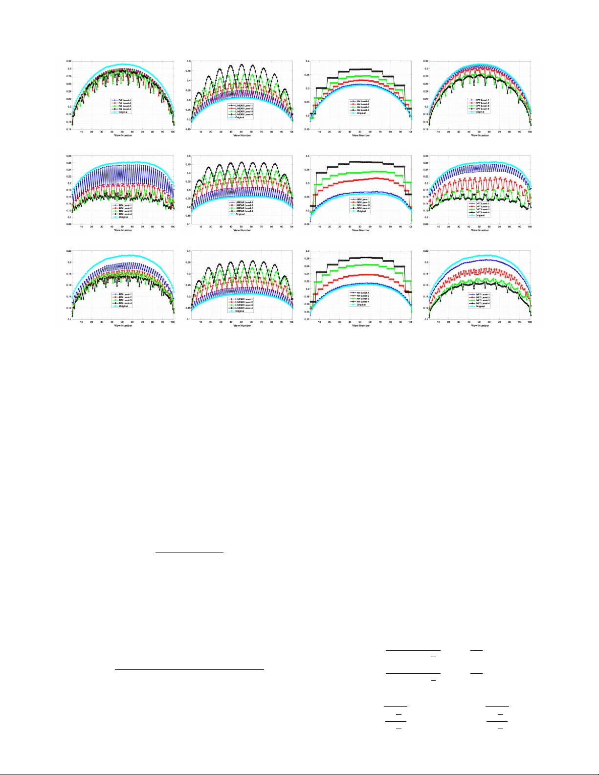
IEEE TRANSA CTIONS ON IMA GE PR OCESSING 1 T ensor Oriented No-Reference Light Field Image Quality Assessment W ei Zhou, Student Member , IEEE , Likun Shi, Zhibo Chen, Senior Member , IEEE , and Jinglin Zhang Abstract —Light field image (LFI) quality assessment is be- coming more and more important, which helps to better guide the acquisition, processing and application of immersive media. Howev er , due to the inherent high dimensional characteristics of LFI, the LFI quality assessment turns into a multi-dimensional problem that requir es consideration of the quality degradation in both spatial and angular dimensions. Therefor e, we propose a novel T ensor oriented No-refer ence Light Field image Quality evaluator (T ensor -NLFQ) based on tensor theory . Specifically , since the LFI is regarded as a low-rank 4D tensor , the principal components of four oriented sub-aperture view stacks are ob- tained via T ucker decomposition. Then, the Principal Component Spatial Characteristic (PCSC) is designed to measure the spatial- dimensional quality of LFI considering its global naturalness and local frequency properties. Finally , the T ensor Angular V ariation Index (T A VI) is proposed to measure angular consistency quality by analyzing the structural similarity distribution between the first principal component and each view in the view stack. Extensive experimental results on four publicly av ailable LFI quality databases demonstrate that the proposed T ensor-NLFQ model outperforms state-of-the-art 2D, 3D, multi-view , and LFI quality assessment algorithms. Index T erms —Light field, image quality assessment, objective model, tensor theory , angular consistency . I . I N T RO D U C T I O N A S an important medium for human visual perception, light enables humans to ef fectively perceive the spa- tial, color , form and dynamic changes of our environment. Con ventional media modalities such as 2D images mainly consider the intensity information of radiance, which can only provide a two-dimensional sense of presence. Different from traditional image capturing formats, light field content records both radiation intensity and direction information of light rays in the free space, thus providing an enhanced immersive experience. Considering the abundant spatial and angular information of the light field, its processing and application hav e attracted widespread attention in past decades. Howe ver , these operations ine vitably introduce heterogeneous artifacts, resulting in the degradation of the perceptual quality for light field content [1]. Therefore, monitoring the perceptual W . Zhou, L. Shi and Z. Chen are with the CAS K ey Laboratory of T echnol- ogy in Geo-Spatial Information Processing and Application System, Univer - sity of Science and T echnology of China, Hefei 230027, China (e-mail: wei- chou@mail.ustc.edu.cn; slikun@mail.ustc.edu.cn; chenzhibo@ustc.edu.cn). J. Zhang is with Key Laboratory of Meteorological Disaster , Ministry of Education, Nanjing University of Information Science and T echnology , Nanjing 210044, China (e-mail: jinglin.zhang@nuist.edu.cn). Corresponding author: Zhibo Chen. W ei Zhou and Likun Shi contributed equally to this paper . This work was supported in part by NSFC under Grant U1908209, Grant 61632001, Grant 41775008, and Grant 61702275, and in part by the National Key Research and Dev elopment Program of China under Grant 2018AAA0101400. quality of light field content is critical to better guiding the procedure of light field acquisition, processing and application techniques. T o facilitate the recording and processing of light field content, a 4D function based on the assumption that the light ray radiance is monochromatic, time-in variant and constant along a straight line is adopted to represent light field data [2], [3]. Specifically , light field is parameterized by four coordinates L ( s, t, x, y ) , where the s, t dimensions are angular dimensions and x, y dimensions denote spatial dimensions. When a 4D light field image (LFI) is captured by L ytro Illum [4], each view in the LFI is called a sub-aperture image (SAI). Due to the high dimensional characteristics of LFI, its quality is influenced by different dimension of impairments than that of traditional media. Therefore, it is necessary to analyze the specific factors in LFI quality assessment. The existing research works based on subjectiv e ev aluation [5]–[9] found that the LFI quality assessment needs to consider from these three aspects, namely spatio-angular resolution, spatial quality , and angular consistency . Specifically , spatio-angular resolution refers to the number of SAIs in a LFI and the resolution of a SAI. Spatial quality indicates the quality of SAIs and angular consistency measures the visual coherence between SAIs. Since the spatio-angular resolution is usually determined by the acquisition devices, this paper focuses on the effects of spatial quality and angular consistency . Although subjective ev aluation is an ef fecti ve way to un- derstand human behavior and provides reliable image quality scores, it is resource and time consuming without the possi- bility to be applied for practical applications. Therefore, an effecti ve objectiv e LFI quality assessment model is necessary . Con ventionally , image quality assessment (IQA) models can be roughly classified into three categories based on the av ail- ability of original reference image information: full-reference (FR), reduced-reference (RR) and no-reference (NR). Howe ver , most of these objectiv e models ignore the intrinsic high dimensional characteristics of LFI. In recent works, the tensor theory has been successfully applied to many fields of computer vision, such as compression and recognition [10]. Mathematically , a LFI belongs to a 4D tensor . Therefore, the tensor theory can effecti vely describe the characteristics and distributions in the high-dimensional space. Moreover , these aforementioned methods are designed to extract features in the luminance domain. Although luminance is considered as a dominant factor for understanding the human visual perception [11], luminance-based IQA methods may be sub- optimal because they underestimate visual interference caused by color distortion, especially the significant differences in the IEEE TRANSA CTIONS ON IMA GE PR OCESSING 2 C o l o r S p a c e C o n v e r s i o n V i e w S t a c k Tu c k e r D e c o m p o s i ti o n P r i n c i p a l C o m p o n e n t S p a ti a l C h a r a c te r i s t i c s ( P C S C ) Te n s o r A n g u l a r V a r i a ti o n I n d e x ( TA V I ) F e a tu r e E x tr a c ti o n Li g h t F i e l d I m a g e ( LF I ) R e g r e s s i o n M o d e l P r e d i c te d Q u a l i ty S c o r e Ev a l u a ti o n 0 o 45 o 90 o 135 o C 1 C 2 C 3 Fig. 1: Flow diagram of the proposed T ensor-NLFQ model. colors of dif ferent SAIs. In addition, existing methods neglect the impact of angular consistency in diverse orientations [12], [13] or only consider horizontal angular consistency [14], [15]. Since the LFI is an image array , the relationship between each SAI and the adjacent SAI can reflect the LFI angular consis- tency . Generally , a SAI has eight adjacent SAIs that correspond to angular consistency in four orientation, namely horizontal, vertical, left diagonal, and right diagonal orientations. In this paper , based on the tensor theory , we proposed a nov el T ensor oriented No-reference Light Field image Quality ev aluator (T ensor-NLFQ), which considers both luminance and chrominance effects, as well as the impact of angular con- sistency in div erse directions on the LFI quality . Specifically , the SAIs in RGB are first conv erted into CIELAB color space, which contains one luminance and two chrominance channels. Second, to comprehensively capture the degradation of LFI angular consistency , view stacks are generated along four orientations. Third, the Tuck er decomposition is employed to reduce the angular dimensional of view stacks and obtain the first principal component as the most important dimensionality reduced image. Fourth, considering that the LFI quality is affected by both the spatial quality and angular consistency , we propose the Principal Component Spatial Characteris- tics (PCSC) for measuring the spatial quality including two key aspects: i) the naturalness distribution of individual and mutual color channels is extracted to measure the global distortion; ii) local frequency distribution is used to capture local spatial quality degradation. In addition, we propose the T ensor Angular V ariation Index (T A VI) to measure the angular consistency , which is computed by analyzing the structural similarity distrib ution between the first principal component and each view in the view stack. Our experimental results show that the performance of our proposed model correlates well with human visual perception and achiev es the state-of- the-art performance. The source codes of T ensor-NLFQ will be av ailable online for public research usage 1 . The remainder of this paper is organized as follows. Section II introduces the related work. In Section III, we present the details of the proposed model. W e then illustrate the experi- mental results in Section IV . Finally , Section V concludes our paper I I . R E L AT E D W O R K The FR IQA approaches utilize the complete reference image information and measure the difference between ref- erence and distorted images. Among a variety of 2D FR IQA methods, structure similarity between reference and distorted images is measured in structural similarity (SSIM) [16], and sev eral of its variants have been proposed, i.e. multi-scale SSIM (MS-SSIM) [17], feature similarity (FSIM) [18], in- formation content weighted SSIM (IW -SSIM) [19], and so on [20]–[22]. The information fidelity criterion (IFC) [23] and visual information fidelity (VIF) [24] measure the degree of information loss of the distorted images relativ e to the reference image. Moreover , the noise quality measure (NQM) [25] and visual signal-to-noise ratio (VSNR) [26] consider the sensitivity of the human visual system (HVS) to different visual signals. Chen et al. [27] proposed a 3D FR IQA algorithm that models the influence of binocular riv alry . For multi-view FR IQA, morphological pyramid decomposition and morphological wavelet decomposition are employed in morphological wavelet peak signal-to-noise ratio (MW -PSNR) [28] and morphological pyramid PSNR (MP-PSNR) [29], [30], respectiv ely . The 3D synthesized vie w image quality metric (3DSwIM) [31] is based on the comparison of statistical features from wav elet subbands. The RR IQA algorithms utilize partial information of the reference image for quality assessment, which is exploited 1 http://staff.ustc.edu.cn/ ∼ chenzhibo/resources.html IEEE TRANSA CTIONS ON IMA GE PR OCESSING 3 when the reference information is transmitted at low band- width, such as [32]–[34]. The NR IQA methods measure dis- torted image quality without needing the original image, which is more applicable in most real-world scenarios. For example, natural scene statistics from different domains are extracted to predict 2D image quality [35]–[39]. For 3D NR IQA, binocular vision theory and depth perception are adopted in several methods [40]–[42]. Gu et al. [43] proposed a multi-view NR IQA algorithm named autoregression (AR)-plus thresholding (APT) that employs the AR-based local image description. Howe ver , none of the aforementioned schemes consider the intrinsic high dimensional characteristics of LFI, especially the distortion caused by angular consistency . Therefore, it is important and necessary to design a new light-field-specific metric. In the literature, sev eral LFI quality assessment models have been proposed. Fang et al. [14] proposed a FR LFI quality assessment method that measures the gradient magnitude similarity of reference and distorted epipolar plane images. Huang et al. [15] also proposed a FR LFI quality assessment algorithm, which is based on dense distortion curve analysis and scene information statistics. The light field image quality assessment metric (LF-IQM) [12] is a RR LFI quality assess- ment metric that assumes the depth map quality is closely related to the LFI overall quality and measures the structural similarity between original and distorted depth maps to predict the perceiv ed LFI quality . Howe ver , Fang [14] and LF-IQM [12] ignore the texture information of SAI, which result in the insufficient measurement of the LFI spatial quality . Further - more, the performance of the LF-IQM is significantly affected by the adopted depth estimation algorithms. Additionally , in most cases, the pristine image is not av ailable, thus NR LFI quality assessment methods are desired. T o the best of our knowledge, our previous work [13] propose the only NR LFI quality assessment metric called blind quality ev aluator of light field image (BELIF), which utilizes binocular vision features for measuring the spatial quality and angular consistency . The differences between BELIF and our proposed T ensor-NLFQ are: 1) The BELIF ignores the effect of chrominance infor- mation. Howe ver , the proposed T ensor-NLFQ method jointly considers both the influence of luminance and chrominance on perceptual quality; 2) The BELIF neglects the effect of local changes in the angular consistency of each direction, while our proposed T ensor-NLFQ exploits the angular consistency of each direction to ev aluate the light field image quality . I I I . P R O P O S E D M E T H O D The framework of T ensor-NLFQ algorithm is illustrated in Fig. 1. First, we con vert SAIs in RGB into CIELAB color space. Second, we exploit T ucker decomposition along angular dimension to generate the principal components of view stacks in diverse orientations. Third, the PCSC and T A VI are extracted to measure the degradation of spatial quality and angular consistency , respecti vely . Finally , we utilize the regression model to predict the perceptual LFI quality . (a) (b) (c) (d) (e) (f) Fig. 2: (a-b) T wo horizontal adjacent distorted SAIs from W in5-LID database [8]; (c-d) The corresponding chrominance a ∗ of (a-b); (e-f) The corresponding chrominance b ∗ of (a-b). A. Color Space Con version As an important and dense natural visual cue, color in- formation helps the human brain to achieve both low-le vel and high-lev el visual perception. Extensiv e research works hav e been conducted towards understanding the effects of luminance and chrominance on image quality [39], [44]–[46]. These works prove that the chrominance information has a promising gain for image quality ev aluation. Therefore, it is reasonable to use the color space information to e valuate LFI spatial quality . Furthermore, in our previous work [8], we hav e found that if there exists a significant difference in the color of different SAIs, this may destroy LFI angular consistency . Fig. 2 shows two horizontal adjacent SAIs with reconstruction artifacts selected from Win5-LID database [8] and the corresponding two chrominance components. W e can see that there exist color differences in the SAIs and the two chrominance components are differentiable, which indicate that color information can measure the deterioration of LFI angular consistency . T o better approximate color perception in the HVS, the color SAIs of each LFI are transformed into the perceptu- ally relev ant CIELAB color space with one luminance ( L ∗ ) and two chrominance ( a ∗ and b ∗ ) channels optimized for quantifying perceptual color difference and more compatible with human perception [47]. Specifically , the luminance L ∗ represents color lightness from black to white. Moreover , a ∗ indicates the position between red/magenta and green, while IEEE TRANSA CTIONS ON IMA GE PR OCESSING 4 (a) (b) (c) (d) Fig. 3: T ucker decomposition components and their energy histograms. The horizontal view stack is taken as an example, which contains 9 horizontal stacks. And the angular resolution of each stack is 9. The top, middle and bottom rows denote the components of C 0 ◦ 1 , C 0 ◦ 2 and C 0 ◦ 3 , respectiv ely . (a) the first principal component; (b) the second principal component; (c) the third principal component; (d) energy distribution of the corresponding decomposition components. b ∗ represents the position between yellow and blue. Therefore, one luminance map array ( C 1 ) and two chrominance map arrays ( C 2 and C 3 ) can be obtained, as shown in the yellow box in Fig. 1. Meanwhile, C 1 , C 2 and C 3 hav e the same spatial resolution and angular resolution as the original LFI. B. V iew Stack In natural, the distribution of light is continuous. Howe ver , for practical usage, the LFI is represented as L ( s, t, x, y ) , where ( s, t ) indicates the view index and is an integer . Therefore, except for the corner and boundary SAIs, the remaining SAIs ha ve eight adjacent vie ws. Generally , based on the assumption that the angular resolution of LFI is S × T , each SAI has an angular consistency of four orientations, i.e. 0 ◦ , 45 ◦ , 90 ◦ , and 135 ◦ . As shown in the blue box in Fig. 1, these angles represent horizontal ( 0 ◦ ), left diagonal ( 45 ◦ ), vertical ( 90 ◦ ), and right diagonal ( 135 ◦ ) orientations. W e then stack the SAIs along four orientations to generate view stack as follows: C 0 ◦ n,s = { C n ( s, 1 , : , :) , C n ( s, 2 , : , :) , ..., C n ( s, T , : , :) } , (1) C 90 ◦ n,t = { C n (1 , t, : , :) , C n (2 , t, : , :) , ..., C n ( S, t, : , :) } , (2) C 45 ◦ n,s + t − 1 = { C n ( s, t, : , :) , C n ( s + 1 , t + 1 , : , :) , ..., C n ( s + min { S − s, T − t } , t + min { S − s, T − t } , : , :) } , (3) C 135 ◦ n,s + t − 1 = { C n ( s, t, : , :) , C n ( s + 1 , t − 1 , : , :) , ..., C n ( s + min { S − s, T − 1 } , t − min { S − s, T − 1 } , : , :) } , (4) where s = 1 , 2 , ..., S and t = 1 , 2 , ..., T represent the angular coordinate. n = 1 , 2 , 3 indicate the luminance and two chrominance channels. For the light field image with an angular resolution of S × T , we extract the view stack in four directions as: 1) Containing S horizontal stacks, and the angular resolution of each stack is T ; 2) Containing T vertical stacks, and the angular resolution of each stack is S ; 3) Containing ( S + T − 1) left diagonal stacks, and the angular resolution of each stack increases from 1 to min { S , T } ; 4) Containing ( S + T − 1) right diagonal stacks, and the angular resolution of each stack increases from 1 to min { S , T } . For example, the angular resolution is 9 × 9 in W in5-LID database, including 9 horizontal stacks, 9 v ertical stacks, 17 left diagonal stacks and 17 right diagonal stacks. C. T ucker Decomposition The view stack is a 3D signal that includes two spatial coordinates and one angular coordinate. W e discover that there IEEE TRANSA CTIONS ON IMA GE PR OCESSING 5 (a) (b) (b) Fig. 4: MSCN coefficients for different HEVC compression levels. The HEVC-QP denotes using HEVC standard with specific quantization parameter (QP), where QP=24, 29, 34, 39, and 44. Higher QP represents lower visual quality . (a) luminance MSCN coefficients d M 0 ◦ 1 ; (b) chrominance MSCN coefficients d M 0 ◦ 2 ; (c) chrominance MSCN coefficients d M 0 ◦ 3 ;. exists a high texture similarity between different images of the vie w stack, indicating that there exists a large redundancy in the angular dimension. T o alleviate this problem, we first adopt tensor decomposition to remove redundant information from the angular dimension. It should be noted that there exist significant differences between Tuck er decomposition and principal component analysis (PCA). According to [10], [48], the Tuck er decomposition can be taken as the higher- order generalizations of PCA or singular value decomposition (SVD). Moreover , the PCA operates on two-dimensional ma- trices, which vectorizes the image and destroys the spatial structure information of the image. Howe ver , the T ucker decomposition decomposes tensors in high-dimensional space that can retain the spatial structure information of the image. Therefore, the T ucker decomposition is used to achie ve dimen- sionality reduction [10]. It decomposes a tensor into a core tensor multiplied by a matrix along each dimension. In other words, we decompose the three-dimensional light field signal into the core tensor and the principal components of spatial and angular dimensions. F or horizontal view stack C 0 ◦ n , we thus have: C 0 ◦ n ≈ G × 1 U 1 × 2 U 2 × 3 U 3 , (5) where G ∈ R R 1 × R 2 × R 3 is the core tensor whose entries illustrate the lev el of interaction between dif ferent components. U 1 ∈ R K 1 × R 1 and U 2 ∈ R K 2 × R 2 are the factor matrices in the spatial dimension. U 3 ∈ R K 3 × R 3 is the angular dimension factor matrix. These matrices are usually orthogonal. In our model, we set K n = R n , where n = 1 , 2 , 3 . The core tensor is trained from each distorted SAI. Then, for C 0 ◦ n , the angular decomposition components can be obtained by multiplying the core tensor with the factor matrices U 1 and U 2 along each mode in the spatial dimension, which can be giv en by: C 0 ◦ n = G × 1 U 1 × 2 U 2 , (6) where C 0 ◦ n ≈ C 0 ◦ n × 3 U 3 . That is, we apply the mode product to the core tensor and the principal components of the spatial dimension, which can obtain angular decomposition components. The purpose of removing U 3 is to realize the reconstruction of spatial information and obtain the decom- position components of angular dimension. Similar to the computation process of C 0 ◦ n , we obtain the angular decom- position components C 45 ◦ n , C 90 ◦ n and C 135 ◦ n of view stacks in other orientations. Specifically , we utilize the alternating least squares method provided by the tensor toolbox [49] to imple- ment the T ucker decomposition. Note that the tensor n-mode product represents different modes of tensor multiplication, which is essentially the multiplication of tensors with different dimensions [10]. In addition, here the factor matrices in T ucker decomposi- tion, which are defined as the principal components [10], rep- resent the stacks in the angular dimension for the decomposed three-dimensional tensor, where the first principal component is the highest energy component and contains fundamental texture information. W e select a sample of LFI from W in5-LID database to show the energy distribution of principal compo- nents in Fig. 3, where (a)-(c) illustrates the first three principal components of C 0 ◦ 1 , C 0 ◦ 2 and C 0 ◦ 3 . Fig. 3 (d) shows the energy histogram distrib ution of the corresponding decomposition components. Here, the top, middle and bottom rows denote the components of C 0 ◦ 1 , C 0 ◦ 2 and C 0 ◦ 3 , respecti vely . Obviously , the texture information and energy mainly concentrate on the first principal component, which represents the basic texture information of the vie w stack. By quantitati ve calculation, we find the first principal component contains more than 70% energy , we thus treat it as the most important dimensionality reduced image. W e define the first principal component of C d n as M d n , where n = 1 , 2 , 3 and d = 0 ◦ , 45 ◦ , 90 ◦ , 135 ◦ . D. F eatur e Extraction and Quality Re gression Since the first principal component contains the basic in- formation about each view stack, it is reasonable to extract features from the first principal component to measure the degradation of LFI spatial quality . Specifically , we first extract the PCSC from the first principal component that utilizes global naturalness and local frequency distribution character- istics to ev aluate the distortion in spatial quality . In addition to spatial quality , angular consistency also affects LFI quality . IEEE TRANSA CTIONS ON IMA GE PR OCESSING 6 (a) (b) (c) (d) Fig. 5: Structure similarity distribution of horizontal view stack. The top row represents the ss 0 ◦ 1 of luminance L channel, while the middle and bottom rows indicate the ss 0 ◦ 2 and ss 0 ◦ 3 of chrominance a and b channels. (a) Different DQ distortion lev els; (b) Different LINEAR distortion lev els; (c) Different NN distortion levels; (d) Different OPT distortion levels. Then, the T A VI is proposed to capture angular consistency distortion by computing the structural similarity between the first principal component and each view in the view stack. 1) Principal Component Spatial Characteristic (PCSC): In general, the naturalness of an image can be effecti vely measured by modeling the locally mean subtracted and con- trast normalized (MSCN) coefficients [35]–[37]. The MSCN has been successfully employed for image processing tasks and can be used to model the contrast-gain masking process in early human vision [37], [50]. In our model, MSCN coefficients can be calculated by: b I ( x, y ) = I ( x, y ) − µ ( x, y ) σ ( x, y ) + 1 , (7) where b I ( x, y ) and I ( x, y ) are the MSCN coefficients and input image (i.e. M d n ) values at the spatial position ( x, y ) . µ ( x, y ) and σ ( x, y ) stand for the local mean and standard de viation in a local patch centered at ( x, y ) . They are computed as: µ ( x, y ) = K X k = − K L X l = − L z k,l I k,l ( x, y ) (8) σ ( x, y ) = v u u t K X k = − K L X l = − L z k,l ( I k,l ( x, y ) − µ ( x, y )) 2 , (9) where z = { z k,l | k = − K, ..., K , l = − L, ..., L } denotes a 2D circularly-symmetric Gaussian weighting function with sampled out 3 standard deviations and rescaled to unit volume. Inspired by [37], we set K = L = 3 in our implementation. T o measure the LFI spatial quality , we first consider the nat- uralness distribution of the principal components of luminance and chrominance (i.e. d M d 1 , d M d 2 and d M d 3 ). Fig. 4 presents the distribution of MSCN coefficients for luminance and chromi- nance principal components with sev eral high efficienc y video coding (HEVC) compression lev els. The HEVC is the video coding standard promoted by the Joint Collaborative T eam on V ideo Coding in 2013, and it is also named H.265 [51]. The results show that the distribution of MSCN coef ficients are very indicative when the LFI suffers from artifacts. Here, the sample of LFI is selected from the W in5-LID database [8]. Since the distribution of MSCN coefficients approxi- mates Gaussian distribution and the asymmetric generalized Gaussian distribution (A GGD) further generalizes the GGD [37], [52], we then utilize the zero-mean AGGD model to qualify the distribution of MSCN coef ficients, which can fit the distribution by: f ( χ ; α, σ 2 l , σ 2 r ) =        α ( β l + β r )Γ( 1 α ) exp ( − ( − x β l ) α ) χ < 0 α ( β l + β r )Γ( 1 α ) exp ( − ( − x β r ) α ) χ > 0 , (10) where β l = σ l s Γ( 1 α ) Γ( 3 α ) and β r = σ r s Γ( 1 α ) Γ( 3 α ) , (11) IEEE TRANSA CTIONS ON IMA GE PR OCESSING 7 and α is the shape parameter controlling the shape of the statistic distrib ution, while σ l and σ r are the scale parameters of left and right sides, respecti vely . Moreover , we compute η as another feature by: η = ( β r − β l ) Γ( 2 α ) Γ( 1 α ) (12) In addition, human visual perception is also affected by the combination of luminance and chrominance channels. Therefore, the joint statistics of MSCN coefficients for the principal components under different channels can also be used to measure the deterioration of image quality . Therefore, we utilize multiv ariate generalized Gaussian distribution (MGGD) [53], [54] to fit the joint distribution, which is defined as: f ( x | M , γ , ϕ ) = 1 | M | 1 2 g γ ,ϕ  x T M − 1 x  , (13) where x ∈ R N and M is an N × N symmetric scatter matrix. γ and ϕ indicate the scale and shape parameters, respecti vely . g γ ,ϕ () is the density generator: g γ ,ϕ ( χ ) = ϕ Γ  N 2   2 1 ϕ π γ  N 2 Γ  N 2 ϕ  e − 1 2 ( χ γ ) ϕ , (14) where χ ∈ R + and Γ is the digamma function. W e adopt the method proposed by Pascal et al. [55] to estimate the parameters of the MGGD model. Considering that the degradation of LFI spatial quality induces the change in the local distribution of principal com- ponents. W e extract the local features of principal components for each color channel. Inspired by [36], block-based discrete cosine transform (DCT) is utilized to measure the distrib ution of local information. Specifically , we adopt the entropy of DCT coefficients without DC value as: E = − L X l H X h ( p lh log ( p lh )) , (15) where L and H represent the width and height of DCT block, respectiv ely . p lh is the DCT coefficient located in ( l , h ) . Note that we compute the entropy from three aspects, namely the whole DCT block, three frequency bands, and three orienta- tions of the DCT block as [36]. Therefore, f P C S C is obtained by concatenating the fitting parameters of A GGD and MGGD as well as three av eraged entropy features. Furthermore, the feature dimension of PCSC is 57, where the entropy feature contains 15 dimensions and the feature dimensions for the MSCN based A GGD parameters as well as MGGD parameters are 36 and 6, respecti vely . There exists significant differences between traditional spatial features such as BRISQUE [37] and our proposed f P C S C . Specifically , the BRISQUE [37] only considers the information distrib ution of a single luminance space. In addition to the luminance information, we also calculate the distribution of chrominance space. Considering the interaction between luminance and chroma information, we calculate the joint distribution MGGD. (a) 0 20 40 60 80 100 120 CF 20 40 60 80 100 120 SI SRC01 SRC02 SRC03 SRC04 SRC05 SRC06 SRC07 SRC08 SRC09 SRC10 (b) (c) 0 20 40 60 80 100 120 CF 20 40 60 80 100 120 SI ArtGallery2 ArtGallery2zoom ArtGallery3 BarcelonaNight Bikes Blob Car Cobblestone FairyCollection Furniture1 Furniture3 LivingRoom Mannequin WorkShop (d) (e) 0 20 40 60 80 100 120 CF 20 40 60 80 100 120 SI Whitesky Table Ladder Chair Tile Flower Grid Sky River Building Car Stone Window Pillars Book Person (f) (g) 0 20 40 60 80 100 120 CF 20 40 60 80 100 120 SI I01 I02 I03 I04 I05 (h) Fig. 6: Database descriptions. (a) Center view of source images for W in5-LID; (b) Distribution of SI and CF for W in5-LID; (c) Center view of source images for MPI-LF A; (d) Distribution of SI and CF for MPI-LF A; (e) Center view of source images for SMAR T ; (f) Distribution of SI and CF for SMAR T ; (g) Center view of source images for V ALID; (h) Distribution of SI and CF for V ALID. 2) T ensor Angular V ariation Index (T A VI): In addition to spatial quality , angular consistency also affects the LFI quality . Usually , angular reconstruction operations, such as interpolation, may break angular consistency . T o measure the degradation of angular consistency , we propose the tensor angular variation index. Specifically , we first compute the structural similarity between each view in the view stack and its corresponding first principal component: ss d n ( i ) = F ( C d n ( i ) , M d n ) , (16) IEEE TRANSA CTIONS ON IMA GE PR OCESSING 8 T ABLE I: Performance Comparison on W in5-LID, MPI-LF A, and SMAR T Databases. Win5-LID MPI-LF A SMAR T T ype Metrics SRCC LCC RMSE OR SRCC LCC RMSE OR SRCC LCC RMSE OR 2D FR PSNR 0.6026 0.6189 0.8031 0.0045 0.8078 0.7830 1.2697 0.0060 0.7045 0.7035 1.5330 0.0195 SSIM [16] 0.7346 0.7596 0.6650 0.0000 0.7027 0.7123 1.4327 0.0060 0.6862 0.7455 1.4378 0.0156 MS-SSIM [17] 0.8266 0.8388 0.5566 0.0000 0.7675 0.7518 1.3461 0.0060 0.6906 0.7539 1.4171 0.0117 FSIM [18] 0.8233 0.8318 0.5675 0.0045 0.7776 0.7679 1.3075 0.0030 0.7811 0.8139 1.2533 0.0039 IW -SSIM [19] 0.8352 0.8435 0.5492 0.0000 0.8124 0.7966 1.2340 0.0030 0.7111 0.7971 1.3024 0.0000 IFC [23] 0.5028 0.5393 0.8611 0.0000 0.7573 0.7445 1.3629 0.0030 0.4827 0.5946 1.7343 0.0156 VIF [24] 0.6665 0.7032 0.7270 0.0000 0.7843 0.7861 1.2618 0.0030 0.0684 0.2533 2.0867 0.0469 NQM [25] 0.6508 0.6940 0.7362 0.0045 0.7202 0.7361 1.3817 0.0060 0.4601 0.5305 1.8285 0.0234 VSNR [26] 0.3961 0.5050 0.8826 0.0182 0.7427 0.5787 1.6651 0.0179 0.5542 0.6289 1.6770 0.0156 HDR-VDP2 [56] 0.5555 0.6300 0.7941 0.0045 0.8608 0.8385 1.1123 0.0000 0.1888 0.3347 2.0327 0.0625 2D NR BRISQUE [37] 0.6687 0.7510 0.5619 0.0000 0.6724 0.7597 1.1317 0.0000 0.8239 0.8843 0.8325 0.0000 NIQE [38] 0.2086 0.2645 0.9861 0.0045 0.0665 0.1950 2.0022 0.0327 0.1386 0.1114 2.1436 0.0547 FRIQUEE [39] 0.6328 0.7213 0.5767 0.0000 0.6454 0.7451 1.1036 0.0000 0.7269 0.8345 0.9742 0.0000 3D FR Chen [27] 0.5269 0.6070 0.8126 0.0091 0.7668 0.7585 1.3303 0.0030 0.6798 0.7722 1.3706 0.0078 3D NR SINQ [41] 0.8029 0.8362 0.5124 0.0000 0.8524 0.8612 0.9939 0.0000 0.8682 0.8968 0.9653 0.0000 BSVQE [42] 0.8179 0.8425 0.4801 0.0000 0.8570 0.8751 0.9561 0.0000 0.8449 0.8992 0.8514 0.0000 Multi-view FR MP-PSNR Full [29] 0.5335 0.4766 0.8989 0.0000 0.7203 0.6730 1.5099 0.0089 0.8449 0.8992 0.8514 0.0000 MP-PSNR Reduc [30] 0.5374 0.4765 0.8989 0.0000 0.7210 0.6747 1.5067 0.0089 0.6716 0.6926 1.5559 0.0117 MW -PSNR Full [28] 0.5147 0.4758 0.8993 0.0000 0.7232 0.6770 1.5023 0.0089 0.6620 0.6505 1.6382 0.0117 MW -PSNR Reduc [28] 0.5326 0.4766 0.8989 0.0000 0.7217 0.6757 1.5048 0.0089 0.6769 0.6903 1.5607 0.0117 3DSwIM [31] 0.4320 0.5262 0.8695 0.0182 0.5565 0.5489 1.7063 0.0119 0.4053 0.4707 1.9032 0.0234 Multi-view NR APT [43] 0.3058 0.4087 0.9332 0.0045 0.0710 0.0031 2.0413 0.0357 0.5105 0.5249 1.8361 0.0234 LFI RR LF-IQM [12] 0.4503 0.4763 0.8991 0.0273 0.3364 0.4223 1.8504 0.0268 0.1222 0.2998 2.0579 0.0547 LFI NR BELIF [13] 0.8719 0.8910 0.4294 0.0000 0.8854 0.9096 0.7877 0.0000 0.8367 0.8833 0.8347 0.0000 Proposed T ensor -NLFQ 0.9101 0.9217 0.3781 0.0000 0.9221 0.9294 0.7241 0.0000 0.8702 0.9028 0.8225 0.0000 T ABLE II: Performance Comparison on V ALID Database. V ALID-8bit V ALID-10bit T ype Metrics SRCC LCC RMSE OR SRCC LCC RMSE OR 2D FR PSNR 0.9620 0.9681 0.3352 0.0000 0.9467 0.9524 0.2935 0.0000 SSIM [16] 0.9576 0.9573 0.3868 0.0000 0.9326 0.9375 0.3348 0.0000 MS-SSIM [17] 0.9593 0.9658 0.3473 0.0000 0.9432 0.9484 0.3051 0.0000 IW -SSIM [19] 0.9674 0.9764 0.2892 0.0000 0.9499 0.9617 0.2638 0.0000 NQM [25] 0.9055 0.9194 0.5266 0.0000 0.8410 0.8582 0.4940 0.0000 HDR-VDP2 [56] 0.9623 0.9785 0.2758 0.0000 0.9371 0.9528 0.2921 0.0000 2D NR BRISQUE [37] 0.9222 0.9849 0.2017 0.0000 0.9027 0.9347 0.2838 0.0000 FRIQUEE [39] 0.9157 0.9836 0.2160 0.0000 0.8559 0.8986 0.3497 0.0000 3D NR SINQ [41] 0.9222 0.9849 0.2070 0.0000 0.9021 0.9348 0.2722 0.0000 Multi-view FR MP-PSNR Full [29] 0.9730 0.9852 0.2291 0.0000 0.3830 0.3582 0.8986 0.0000 MP-PSNR Reduc [30] 0.9744 0.9859 0.2237 0.0000 0.3826 0.3506 0.9013 0.0000 MW -PSNR Full [28] 0.9597 0.9677 0.3376 0.0000 0.3764 0.3556 0.8995 0.0000 MW -PSNR Reduc [28] 0.9648 0.9751 0.2970 0.0000 0.3815 0.3563 0.8993 0.0100 3DSwIM [31] 0.7950 0.7876 0.8248 0.0000 0.7869 0.7401 0.6472 0.0000 LFI RR LF-IQM [12] 0.3934 0.5001 1.1593 0.0000 0.3679 0.3705 0.8939 0.0100 LFI NR BELIF [13] 0.9278 0.9862 0.1680 0.0000 0.9186 0.9622 0.2387 0.0000 Proposed T ensor -NLFQ 0.9286 0.9852 0.1825 0.0000 0.9367 0.9640 0.2295 0.0000 where C d n is the input view stack and M d n represents the corresponding first principal component. i indicates the an- gular coordinate of C . n = 1 , 2 , 3 and d = 0 ◦ , 45 ◦ , 90 ◦ , 135 ◦ represent the index of three color channels and four orienta- tions, respectiv ely . F is the function to calculate the structural similarity between C d n ( i ) and M d n . In our paper, we use the SSIM [16]. The structure similarity distribution of LFI selected from MPI-LF A [7] is illustrated in Fig. 5. For information with only horizontal direction, we only use horizontal direction features and the weight of other directions feature is 0. As shown in Fig. 5, the horizontal vie w stack can also reflect the change of angular consistency . In other words, since the MPI-LF A database contains only horizontal LFIs, Fig. 5 only presents the structure similarity distribution of the horizontal view stack. The top row represents the ss 0 ◦ 1 of luminance L channel, while the middle and bottom rows indicate the ss 0 ◦ 2 and ss 0 ◦ 3 of chrominance a and b channels, respectiv ely . Fig. 5(a-d) show the structure similarity distribution of original LFI and the distribution of different distortion levels for quantized depth maps (DQ), linear interpolation (LINEAR), nearest interpolation (NN), and image warping using optical flow estimation (OPT) artifacts. It can be seen that when the angular consistency is not destroyed, the distribution of IEEE TRANSA CTIONS ON IMA GE PR OCESSING 9 (a) (b) Fig. 7: Scatter plots of predicted quality scores by three methods against the MOS values on the Win5-LID and MPI-LF A databases. The horizontal and vertical axes in each figure represent the predicted quality scores and MOS values, respecti vely . The red line is the fitted curve. The top, middle and bottom rows are the results of IW -SSIM, BELIF and the proposed model, respectively . (a) Scatter plots on W in5-LID database; (b) Scatter plots on MPI-LF A database. structural similarity is smooth, as shown the cyan curve in Fig. 5. Howe ver , when the angular consistency is degraded by interpolation distortion, the distribution of structural similarity changes significantly . Specifically , as the angular consistency deteriorates, the variation degree in the structural similarity distribution of the LFI increases gradually . Moreover , different distortions types have different wav e shapes. For example, the NN distortion is stepped and the LINEAR distortion has more peaks. These demonstrate that the structure similarity distribution is good at distinguishing various distortion types and levels. Then, inspired by Fig. 5, we employ a second-order poly- nomial to fit the structure similarity distribution as follows: ss d n ( i ) = f 1 i 2 + f 2 i + f 3 , (17) where i is the angular coordinate. f 1 , f 2 and f 3 are fitting parameters modeling variation of angular consistency . T o further characterize the structure similarity properties, we extract sev eral complementary features including contrast, angular second moment, entropy and inv erse different moment [57] to represent the deterioration information. Specifically , the contrast is the amount of local variation presented in structure 10 20 30 40 50 60 70 80 90 Training percentage (%) 0.5 0.55 0.6 0.65 0.7 0.75 0.8 0.85 0.9 0.95 Median value SRCC LCC (a) 10 20 30 40 50 60 70 80 90 Training percentage (%) 0.4 0.5 0.6 0.7 0.8 0.9 1 Median value SRCC LCC (b) Fig. 8: The change of performance results for T ensor-NLFQ with different training and testing percentages. (a) Run on W in5-LID database; (b) Run on MPI-LF A database. similarity . The angular second moment and in verse different moment measure the homogeneity . Thus, f T AV I is obtained by concatenating the fitting parameters (i.e. f 1 , f 2 , f 3 ) and the complementary features. The dimension of feature T A VI is 30. 3) Direction P ooling: For a LFI with an angular resolution of S × T , we have S horizontal view stacks, T vertical view stacks, S + T − 1 main-diagonal view stacks and S + T − 1 secondary-diagonal vie w stacks. Since we extract the features of the view stack in each orientation and average the features from the stack in the same orientation, the f d is first obtained by concatenating f P C S C and f T AV I in the same orientation and d = 0 ◦ , 45 ◦ , 90 ◦ , 135 ◦ . W e then model the final features by: f f inal = w 1 f 0 ◦ + w 2 f 45 ◦ + w 3 f 90 ◦ + w 4 f 135 ◦ , (18) where w 1 , w 2 , w 3 and w 4 indicate the corresponding weights of four orientations. In our model, we set w 1 = w 2 = w 3 = w 4 = 1 4 . The final results are trained with the average features from each stack in the same orientation, and then all directions are weighted. Finally , in this model, we train a regression model to map the final feature vector f f inal space to quality scores. In our implementation, we adopt the well-known support vector regression (SVR), which has been effecti vely applied to many image quality assessment problems [41], [42], [58]. Specifi- cally , the LIBSVM package [59] is utilized to implement the SVR with a radial basis function kernel. I V . E X P E R I M E N TA L R E S U LT S T o validate our proposed T ensor-NLFQ model, we conduct experiments on four publicly available databases, namely W in5-LID [8], MPI-LF A [7], SMAR T [5] and V ALID [60]. As shown in Fig. 6(a) and Fig. 6(b), the Win5-LID database contains 6 real scenes captured by L ytro illum and 4 synthetic scenes as original images which cov er various spatial percep- tual information (SI) and colorfulness (CF) [61]. There exist 220 distorted LFIs by introducing 6 distortion types, including HEVC, JPEG, LINEAR, NN and two CNN models. Moreover , more than 20 observers are invited to provide subjecti ve ratings for the 220 distorted LFIs under the double-stimulus continuous quality scale on a 5-point discrete scale. Therefore, IEEE TRANSA CTIONS ON IMA GE PR OCESSING 10 T ABLE III: RMSE Performance of Different Distortion T ypes on W in5-LID and MPI-LF A Databases. Win5-LID MPI-LF A T ype Metrics HEVC JPEG LINEAR NN HEVC DQ OPT LINEAR NN GA USS 2D FR PSNR 0.6404 0.5219 0.5233 0.3843 0.9496 1.1390 1.3430 0.9156 0.7667 0.7894 SSIM [16] 0.3808 0.5324 0.4414 0.4252 0.5578 1.5566 1.4087 1.2695 1.0692 0.4188 MS-SSIM [17] 0.2515 0.4272 0.4167 0.4170 0.4488 1.2445 1.3018 1.0766 0.7961 0.5049 FSIM [18] 0.2564 0.4377 0.4062 0.4009 0.5091 1.0886 1.2849 1.0537 0.8142 0.6747 IW -SSIM [19] 0.2559 0.4133 0.3702 0.4187 0.4936 1.0900 1.1853 0.8957 0.6105 0.5343 IFC [23] 0.5396 0.6433 0.7092 0.4472 0.8244 0.8882 1.1915 0.8121 0.6229 0.9893 VIF [24] 0.2792 0.4351 0.4554 0.3712 0.4336 1.2041 1.4072 0.8385 0.7069 0.6535 NQM [25] 0.4952 0.6062 0.6228 0.5248 0.6618 1.3064 1.4238 1.1291 0.6228 0.7660 VSNR [26] 0.4460 0.4585 0.9115 0.7314 0.3249 1.7150 1.5878 1.6959 1.3126 0.6930 HDR-VDP2 [56] 0.4460 0.4585 0.9115 0.7314 0.3249 1.7150 1.5878 1.6959 1.3126 0.6930 2D NR BRISQUE [37] 0.2695 0.2225 0.3230 0.4018 0.3468 0.7297 0.8132 0.7577 0.7733 0.4301 NIQE [38] 0.9978 0.9686 0.8986 0.7594 1.0622 1.7489 1.7262 2.0515 1.6397 1.9197 FRIQUEE [39] 0.4127 0.2273 0.3285 0.3748 0.2605 0.6906 0.8170 0.8067 0.8002 0.2551 3D FR Chen [27] 0.2341 0.3795 0.8978 0.6077 0.4763 1.2547 1.3122 1.0762 0.8093 0.4824 3D NR SINQ [41] 0.2373 0.2169 0.2846 0.3419 0.1638 0.5996 0.8109 0.6511 0.7078 0.3432 BSVQE [42] 0.2943 0.2300 0.3199 0.2628 0.3128 0.6877 0.8255 0.6571 0.4864 0.2309 Multi-view FR MP-PSNR Full [29] 0.5357 0.5216 0.7325 0.4318 0.7634 0.9989 1.1191 0.7106 0.6670 0.9100 MP-PSNR Reduc [30] 0.4592 0.5119 0.7331 0.4255 0.9392 0.9998 1.1181 0.7179 0.6608 0.9201 MW -PSNR Full [28] 0.5857 0.5511 0.7329 0.4291 0.8729 1.0013 1.1155 0.6957 0.6426 0.7260 MW -PSNR Reduc [28] 0.4762 0.5326 0.7329 0.4313 0.8056 0.9980 1.1135 0.7130 0.6519 0.7572 3DSwIM [31] 0.9778 0.7278 0.6160 0.4536 1.9656 1.2155 1.4833 1.2782 1.2013 1.5171 Multi-view NR APT [43] 0.9788 0.9757 0.7731 0.7196 2.2549 1.7238 1.6306 2.0857 1.6486 1.9675 LFI RR LF-IQM [12] 1.0987 0.8029 0.6096 0.5409 1.8225 1.7211 1.7645 1.9623 1.5168 1.3558 LFI NR BELIF [13] 0.3062 0.2013 0.3187 0.3052 0.2486 0.6513 0.8023 0.4472 0.3556 0.1527 Proposed T ensor -NLFQ 0.2578 0.1902 0.2633 0.1974 0.2030 0.5370 0.7970 0.3555 0.3125 0.1597 each LFI has the overall mean opinion score (MOS) value, which is a statistical concept as the ground truth image quality measurement. The MOS is calculated by the mean subjective ratings of each LFI. As we can see from Fig. 6(c) and Fig. 6(d), the MPI- LF A database consists of 14 pristine LFIs captured by the TSC system, which also co ver various SI and CF . The 336 distorted LFIs are produced with 6 distortion types, i.e. HEVC, DQ, OPT , LINEAR, NN and GA USS. In order to assess the LFI quality , the pair-wise comparison (PC) method with a two-alternati ve-forced-choice is carried out and the just- objectionable-differences value is pro vided, which is similar to the difference-mean-opinion-score value. Fig. 6(e) and Fig. 6(f) shows the original images and their distribution of SI and CF for the SMAR T database. This database is composed of 16 original LFIs and 256 distorted sequences are obtained by introducing 4 compression distortions which include HEVC Intra, JPEG, JPEG2000 as well as Sparse Set and Disparity Coding. Similarly , the PC method is exploited to collect the subjectiv e ratings and the Bradley-T erry scores are provided. The V ALID database has 5 reference LFIs and 40 distorted LFIs under 5 compression artifacts. Fig. 6(g) and Fig. 6(h) shows the original images and the corresponding SI and CF distribution. Note that the V ALID database includes both 8bit and 10bit LFIs. The comparison-based adjectiv al categorical judgement methodology is used to 8bit images, while the double stimulus impairment scale is performed for 10bit images. In addition, the MOS values are provided for the LFIs. T o ev aluate the model performance on these databases, we choose four ev aluation criteria, including Spearman rank-order T ABLE IV: Performance Results of Synthetic and Real Scenes for T ensor-NLFQ on Win5-LID Database. Methods SRCC LCC RMSE Synthetic scene 0.8837 0.9314 0.3339 Real scene 0.8834 0.9144 0.3429 T ABLE V: Comparison Results of T ucker Decomposition and PCA on W in5-LID Databse. Methods SRCC LCC RMSE PCA 0.8858 0.8962 0.4166 T ucker decomposition (Proposed) 0.9101 0.9217 0.3781 correlation coef ficient (SRCC), linear correlation coefficient (LCC), root mean square error (RMSE) and outlier ratio (OR). The SRCC measures the monotonicity , while LCC focuses on the linear relationship. The RMSE and OR provide the measure of prediction accuracy and consistency , respectiv ely . Higher SRCC and LCC values as well as lo wer RMSE and OR values represent better performance. Before computing LCC, RMSE and OR, a nonlinear function is adopted as: f ( q ) = β 1 { 1 2 − 1 1 + exp [ β 2 ( q − β 3 )] } + β 4 q + β 5 (19) where q is the output of a specific objecti ve metric. The param- eters β 1 ··· 5 are optimized to minimize the giv en goodness-of-fit measure. Additionally , each database is randomly divided into 80% for training and the remaining 20% for testing. W e perform 1000 iterations of cross validation on each database. W e also IEEE TRANSA CTIONS ON IMA GE PR OCESSING 11 T ABLE VI: Performance of Individual Color Channels on W in5-LID and MPI-LF A Databases. Win5-LID MPI-LF A Channel SRCC LCC RMSE SRCC LCC RMSE L 0.8693 0.8838 0.4438 0.8997 0.9066 0.8341 a ∗ 0.7574 0.7638 0.6210 0.8299 0.8468 1.0367 b ∗ 0.8484 0.8592 0.5038 0.8883 0.8845 0.9197 Proposed 0.9101 0.9217 0.3781 0.9221 0.9294 0.7241 T ABLE VII: Performance of Four Direction V iew Stacks on W in5-LID Database. Win5-LID Orientation SRCC LCC RMSE Horizontal 0.8850 0.8994 0.3947 V ertical 0.8529 0.8653 0.4541 Left diagnoal 0.8795 0.8942 0.3944 Right diagnoal 0.8819 0.8894 0.4271 Proposed 0.9101 0.9217 0.3781 T ABLE VIII: Performance of Different Structure Similarity Methods on W in5-LID and MPI-LF A Databases. Win5-LID MPI-LF A Method SRCC LCC RMSE SRCC LCC RMSE SSIM [16] 0.9101 0.9217 0.3781 0.9221 0.9294 0.7241 MS-SSIM [17] 0.9026 0.9159 0.3755 0.9305 0.9300 0.7282 FSIM [18] 0.8876 0.9087 0.4029 0.9227 0.9268 0.7743 IW -SSIM [19] 0.8981 0.9149 0.3834 0.9268 0.9288 0.7368 provide the median SRCC, LCC, RMSE and OR values as the final measurement. A. Comparison with Other Objective Metrics In order to prove the effecti veness of our proposed T ensor- NLFQ model, we conduct fully experiments by using e xist- ing 2D, 3D image, multi-view and LFI quality assessment algorithms. Specifically , we compare with ten 2D FR IQA metrics [16]–[19], [23]–[26], [56], three 2D NR IQA metrics [37]–[39], one 3D FR IQA metric [27], two 3D NR IQA metrics [41], [42], fiv e multi-view FR IQA metrics [28]–[31], one multi-view NR IQA metric [43], one RR LFI quality assessment metric [12], and one NR LFI quality assessment metric [13]. T ABLE I shows the ov erall performance of state-of-the-art objectiv e models on the Win5-LID, MPI-LF A and SMAR T databases, where bold values indicate the best performance results. In T ABLE I, the FR approaches are modeled by formulas, while NR methods are supervised learning algo- rithms except for NIQE [38]. Furthermore, all these learning- based methods are trained by the same percentages with the proposed algorithm on each database. As shown in this table, our proposed T ensor-NLFQ achieves superior performance compared with state-of-the-art algorithms. One possible expla- nation is that existing 2D and 3D IQA approaches only focus on spatial quality rather than angular consistency . Although multi-view IQA metrics consider distortion caused by angular interpolation, they aim to deal with the hole distortion caused by the synthesis. Thus, it is not possible to ef fectiv ely measure LFI artifacts, such as compression distortion. The LFI-IQM [12] method ignores the spatial texture information. Moreover , the LFI-IQM [12] is influenced by depth map estimation, while BELIF [13] cannot take into account the chrominance effects and div erse directions of LFIs. Therefore, their performance is worse than that of the proposed method. T ABLE IX: Performance of Proposed Quality Components on Win5-LID and MPI-LF A Databases. Win5-LID MPI-LF A Featur es SRCC LCC RMSE SRCC LCC RMSE f P C S C 0.8001 0.8188 0.5821 0.8749 0.8815 0.8345 f T AV I 0.8318 0.8521 0.4648 0.7912 0.7964 1.1669 Proposed 0.9101 0.9217 0.3781 0.9221 0.9294 0.7241 T ABLE X: Cross V alidation Results. W e Train Our Proposed Model on W in5-LID and T est on MPI-LF A. SRCC LCC RMSE Proposed 0.8469 0.8192 0.3282 Further , we provide the performance comparison on the V ALID database which includes both 8bit and 10bit LFIs. The V ALID database only has 5 original LFIs, whose SI and CF distribution is relatively concentrated. As we can see from T ABLE II, the proposed T ensor-NLFQ deliv ers good performance values and especially outperforms state-of-the-art NR IQA algorithms for 10bit LFIs. T o illustrate the prediction results more clearly , the scatter plots of two existing metrics and the proposed model on the W in5-LID and MPI-LF A databases are shown in Fig. 7. Since the points of our proposed method are more centralized than that of the other metrics, the predictions of our proposed T ensor-NLFQ are more consistent with subjective quality scores. In addition, Fig. 8 shows the change of performance results for our proposed T ensor -NLFQ method with respect to the training and testing percentages. W e can observe that a large number of training data generally bring about the increase of SRCC and LCC performance on both W in5- LID and MPI-LF A databases, which is consistent with [42]. Moreov er , we choose 80%-20% for the training-testing split since this is a common practice in quality assessment [35], [36]. Besides direct performance comparisons, we also quanti- tativ ely evaluate the statistical significance using the t-test [37] based on the SRCC values obtained from 1000 train-test trials. Here, the null hypothesis is that the mean correlation for the proposed method is equal to that for the compared state-of-the-art algorithm with a confidence of 95%. The experimental results demonstrate that our proposed T ensor- NLFQ significantly outperforms state-of-the-art objective IQA algorithms. B. Robustness Against Distortion and Data T ypes Since the W in5-LID and MPI-LF A in volv e various dis- tortion types, it is interesting to know how our proposed IEEE TRANSA CTIONS ON IMA GE PR OCESSING 12 T ABLE XI: Performance Comparison of The Computation T ime against SRCC, LCC, RMSE and OR on Win5-LID Database. T ype Metrics T otal Computation Time (s) SRCC LCC RMSE OR 2D FR PSNR 0.8188 0.6026 0.6189 0.8031 0.0045 SSIM [16] 2.3068 0.7346 0.7596 0.6650 0.0000 MS-SSIM [17] 3.2937 0.8266 0.8388 0.5566 0.0000 FSIM [18] 14.4056 0.8233 0.8318 0.5675 0.0045 IW -SSIM [19] 27.0113 0.8352 0.8435 0.5492 0.0000 IFC [23] 69.5933 0.5028 0.5393 0.8611 0.0000 VIF [24] 65.9176 0.6665 0.7032 0.7270 0.0000 NQM [25] 16.5390 0.6508 0.6940 0.7362 0.0045 VSNR [26] 4.0910 0.3961 0.5050 0.8826 0.0182 HDR-VDP2 [56] 115.1300 0.5555 0.6300 0.7941 0.0045 2D NR BRISQUE [37] 4.4593 0.6687 0.7510 0.5619 0.0000 NIQE [38] 8.8498 0.2086 0.2645 0.9861 0.0045 FRIQUEE [39] 2343.0336 0.6328 0.7213 0.5767 0.0000 3D FR Chen [27] 1239.3772 0.5269 0.6070 0.8126 0.0091 3D NR SINQ [41] 309.7299 0.8029 0.8362 0.5124 0.0000 BSVQE [42] 396.6745 0.8179 0.8425 0.4801 0.0000 Multi-view FR MP-PSNR Full [29] 32.2917 0.5335 0.4766 0.8989 0.0000 MP-PSNR Reduc [30] 16.2708 0.5374 0.4765 0.8989 0.0000 MW -PSNR Full [28] 1.1421 0.5147 0.4758 0.8993 0.0000 MW -PSNR Reduc [28] 1.1352 0.5326 0.4766 0.8989 0.0000 3DSwIM [31] 322.9451 0.4320 0.5262 0.8695 0.0182 Multi-view NR APT [43] 2626.8449 0.3058 0.4087 0.9332 0.0045 LFI RR LF-IQM [12] 1168.7424 0.4503 0.4763 0.8991 0.0273 LFI NR Proposed NR-LFQA 865.0019 0.9032 0.9206 0.3876 0.0000 model performs for individual distortion types. The perfor- mance results for each separate distortion type are listed in T ABLE III. Due to the space constraints, we only sho w RMSE results. It can be seen that our proposed T ensor- NLFQ method outperforms existing objectiv e metrics for most distortion types. Moreover , the proposed model achieves the best performance for typical reconstruction distortions because the reconstruction distortion mainly destroys angle consistency and usually has little influence on spatial quality . Therefore, existing IQA models are difficult to handle such distortions. Although HEVC compression distortion and Gaussian blur mainly cause the degradation of spatial quality , our T ensor- NLFQ is still very competitiv e and has a good performance. The JPEG distortion in Win5-LID is introduced based on lenslet, and it affects both spatial quality and angular con- sistency of LFI. The proposed method considers the effects of both two factors, it is thus not surprising that our model obtains the best performance for JPEG distorted LFIs. Overall, the proposed T ensor-NLFQ can achieve promising performance against existing objective ev aluation algorithms regarding to various distortion types. In addition to different distortion types, we test the perfor- mance of our proposed T ensor-NLFQ method on synthetic and real scenes separately . As shown in T ABLE IV, the proposed T ensor-NLFQ can handle both synthetic and real scenes. C. V alidity of T ucker Decomposition According to [10], [48], the T ucker decomposition can be regarded as the higher-order generalizations of PCA or SVD. Since the SVD operation generates huge matrices that make computation difficult, we thus adopt the PCA for performance comparison. Specifically , we reshape LFIs as matrices and then use PCA. The experimental results are shown in T ABLE V. From T ABLE V, we can see that our proposed T ucker decom- position outperforms PCA. This is because the tensor-based approach preserves the correlation of spatial information. D. V alidity of Individual Color Channel Since the luminance and chrominance features of LFI are utilized in the proposed model, it is necessary to kno w how much contribution each color channel has. T ABLE VI exhibits the performance of individual color channels on Win5-LID and MPI-LF A databases. It can be seen that the luminance channel achieves the best performance among three color channels, which prov es that the luminance has the most important influence on LFI quality . Moreover , it is observed that two chrominance channels deliver good performance on two databases, which demonstrates that chrominance also has a significant impact on LFI quality . E. V alidity of Single Orientation V iew Stack In the proposed T ensor-NLFQ method, we weight the ex- tracted features of four orientation view stacks to predict the LFI overall quality . It is meaningful to verify the performance of the view stack in each orientation. Since the MPI-LF A database only includes the horizontal view stack, we present the results on the Win5-LID database, as shown in T ABLE VII. W e can observe that for 4D LFIs, the view stack in each direction has a good performance, which indicates that the characteristics of each orientation can reflect the LFI quality to some extent. Meanwhile, the performance of the final model with four directional feature weighting is significantly improv ed. IEEE TRANSA CTIONS ON IMA GE PR OCESSING 13 T ABLE XII: Performance Results of The Computation Time for T ensor-NLFQ with Different LFI dimensions on W in5-LID Database. L ( s, t, x, y ) T otal Computation Time (s) L (9 , 9 , 434 , 625) 865.0019 L (5 , 5 , 434 , 625) 361.7581 L (3 , 3 , 434 , 625) 186.2238 L (9 , 9 , 217 , 313) 200.4934 L (9 , 9 , 145 , 208) 99.4762 L (5 , 5 , 217 , 313) 94.0500 F . Differ ent Structur e Similarity Methods In the T A VI measurement, we use SSIM [16] as an al- gorithm for measuring structure similarity . Except for SSIM, sev eral variants of SSIM hav e been proposed, such as MS- SSIM [17], FSIM [18] and IW -SSIM [19]. Therefore, we wonder how the proposed method performs when we adopt these algorithms. T ABLE VIII illustrates the results of our proposed model using dif ferent structure similarity methods on W in5-LID and MPI-LF A databases, which indicates that our T ensor-NLFQ model does not rely much on specific structural similarity algorithms. G. V alidity of Individual Pr oposed F eature In this section, we explore the validity of two proposed fea- tures (i.e. f P C S C and f T AV I ) of our model. The performance values of these two features are shown in T ABLE IX. It can be seen that f P C S C has a good performance on both databases due to the effecti veness of measuring spatial quality , especially on the MPI-LF A database. The reason may be that some interpolation operations in the MPI-LF A database can also cause the degradation of spatial quality . Therefore, in addition to capture the deterioration of spatial quality , f P C S C can also measure a certain degree of angular distortion. Furthermore, f T AV I deliv ers the slightly lower performance on the MPI- LF A database. Since the MPI-LF A database contains many angular distorted LFIs with low distortion lev els and the qual- ity difference is small, human is insensiti ve to these sequences. Howe ver , the proposed f T AV I can capture the degradation of angular consistency effecti vely . This phenomenon can be shown in Fig. 5, where the curve of distortion sequences are significantly different. Overall, the results validate our proposed features and the performance is improved after the feature combination. H. Model Generality and T ime Complexity T o v alidate the model generality , we choose the same distortion in the MPI-LF A and W in5-LID databases to conduct experiments. Specifically , we train the proposed T ensor-NLFQ on the W in5-LID database, and then test it on the LFIs with the same distortion in the MPI-LF A database. The results are shown in T ABLE X. W e can observe that the proposed model is independent for the adopted database. In addition, we compare the proposed T ensor-NLFQ method with state-of-the-art quality assessment approaches for com- putational complexity on the W in5-LID database. It should be noted that we also list the SRCC, LCC, RMSE and OR for fair comparison. As shown in T ABLE XI, our proposed T ensor- NLFQ is demonstrated to hav e lower computation time com- pared to LF-IQM [12]. The reason may be that dif ferent from con ventional LFI quality assessment metrics, our proposed approach relieves the complex computation for estimating depth maps. In general, our proposed T ensor-NLFQ method is in the same lev el of time complexity compared with state-of- the-art 3D quality assessment metrics and demonstrates the best SRCC, LCC, RMSE and OR performance among all algorithms. Further, we analyze the effects of different angular and spatial dimensions on time complexity . Specifically , we sample the LFI in angular and spatial dimensions by 1 / 2 and 1 / 3 times separately . The LFI is also sampled in angular and spatial dimensions by 1 / 2 times simultaneously . The performance results are shown in T ABLE XII. W e can see that the time complexity of our proposed T ensor-NLFQ is affected by the angular and spatial dimensions of LFIs. The reduction of angular and spatial dimensions significantly reduces the computation time. V . C O N C L U S I O N In this paper, we present a novel T ensor oriented No- reference Light Field image Quality ev aluator (T ensor-NLFQ). According to the existing research and our previous work, color information has a significant impact on the perceiv ed LFI quality . W e thus introduce luminance and chrominance information in our proposed model. Since the LFI can be regarded as a high-dimensional tensor signal, we exploit the tensor decomposition to extract the principal components of LFI, which can effecti vely reflect the LFI quality . The angular consistency of div erse directions is considered in the proposed method, including horizontal, diagonal, vertical and right di- agonal orientations. As the LFI quality is affected by both spatial quality and angular consistency , we propose principal component spatial characteristic and tensor angular variation index to measure the degradation of spatial quality and angular consistency , respectively . W e conduct extensi ve experiments to compare the proposed T ensor-NLFQ with existing 2D, 3D image, multi-view and LFI quality assessment algorithms. The results demonstrate that our approach outperforms state-of-the- art metrics and can handle the typical distortions of LFI. In the future, we will extend the proposed model to light field video quality assessment. Moreover , ho w to apply our proposed method to the optimization of existing image com- pression and reconstruction algorithms could also be further explored. R E F E R E N C E S [1] G. W u, B. Masia, A. Jarabo, Y . Zhang, L. W ang, Q. Dai, T . Chai, and Y . Liu, “Light field image processing: An overvie w , ” IEEE Journal of Selected T opics in Signal Pr ocessing , vol. 11, no. 7, pp. 926–954, 2017. [2] M. Le voy and P . Hanrahan, “Light field rendering, ” in Proceedings of the 23rd annual conference on Computer graphics and interactive techniques . A CM, 1996, pp. 31–42. [3] S. J. Gortler, R. Grzeszczuk, R. Szeliski, and M. F . Cohen, “The lumigraph, ” in Pr oceedings of the 23rd annual conference on Computer graphics and interactive techniques . A CM, 1996, pp. 43–54. [4] Lytro, http://www .lytro.com, 2017.[Online]. IEEE TRANSA CTIONS ON IMA GE PR OCESSING 14 [5] P . Paudyal, F . Battisti, M. Sj ¨ ostr ¨ om, R. Olsson, and M. Carli, “T owards the perceptual quality evaluation of compressed light field images, ” IEEE T ransactions on Broadcasting , vol. 63, no. 3, pp. 507–522, 2017. [6] I. V iola, M. Rerabek, and T . Ebrahimi, “Comparison and ev aluation of light field image coding approaches, ” IEEE Journal of selected topics in signal processing , vol. 11, no. EPFL-AR TICLE-230995, 2017. [7] V . K. Adhikarla, M. V inkler , D. Sumin, R. K. Mantiuk, K. Myszkowski, H.-P . Seidel, and P . Didyk, “T owards a quality metric for dense light fields, ” in Computer V ision and P attern Recognition (CVPR), 2017 IEEE Confer ence on . IEEE, 2017, pp. 3720–3729. [8] L. Shi, S. Zhao, W . Zhou, and Z. Chen, “Perceptual ev aluation of light field image, ” in 2018 25th IEEE International Conference on Image Pr ocessing (ICIP) , Oct 2018, pp. 41–45. [9] P . A. Kara, P . T . Ko vacs, S. V agharshakyan, M. G. Martini, A. Barsi, T . Balogh, A. Chuchvara, and A. Chehaibi, “The effect of light field reconstruction and angular resolution reduction on the quality of expe- rience, ” in Signal-Image T echnology & Internet-Based Systems (SITIS), 2016 12th International Confer ence on . IEEE, 2016, pp. 781–786. [10] T . G. Kolda and B. W . Bader, “T ensor decompositions and applications, ” SIAM re view , vol. 51, no. 3, pp. 455–500, 2009. [11] W . Lin and C.-C. J. Kuo, “Perceptual visual quality metrics: A survey , ” Journal of V isual Communication and Image Repr esentation , vol. 22, no. 4, pp. 297–312, 2011. [12] P . Paudyal, F . Battisti, and M. Carli, “Reduced reference quality assess- ment of light field images, ” IEEE Tr ansactions on Broadcasting , v ol. 65, no. 1, pp. 152–165, 2019. [13] L. Shi, S. Zhao, and Z. Chen, “BELIF: Blind quality ev aluator of light field image with tensor structure variation index, ” in 2019 26th IEEE International Conference on Image Processing (ICIP) , 2019, Accepted. [14] Y . Fang, K. W ei, J. Hou, W . W en, and N. Imamoglu, “Light filed image quality assessment by local and global features of epipolar plane image, ” in 2018 IEEE F ourth International Confer ence on Multimedia Big Data (BigMM) . IEEE, 2018, pp. 1–6. [15] Z. Huang, M. Y u, H. Xu, Y . Song, H. Jiang, and G. Jiang, “New quality assessment method for dense light fields, ” in Optoelectronic Imaging and Multimedia T echnology V , vol. 10817. International Society for Optics and Photonics, 2018, p. 1081717. [16] Z. W ang, A. C. Bovik, H. R. Sheikh, and E. P . Simoncelli, “Image quality assessment: from error visibility to structural similarity , ” IEEE T ransactions on image processing , vol. 13, no. 4, pp. 600–612, 2004. [17] Z. W ang, E. P . Simoncelli, and A. C. Bovik, “Multiscale structural simi- larity for image quality assessment, ” in Signals, Systems and Computers, 2004. Confer ence Recor d of the Thirty-Seventh Asilomar Confer ence on , vol. 2. Ieee, 2003, pp. 1398–1402. [18] L. Zhang, L. Zhang, X. Mou, and D. Zhang, “FSIM: A feature similarity index for image quality assessment, ” IEEE T ransactions on Image Pr ocessing , vol. 20, no. 8, pp. 2378–2386, 2011. [19] Z. W ang and Q. Li, “Information content weighting for perceptual image quality assessment, ” IEEE Tr ansactions on Image Processing , vol. 20, no. 5, pp. 1185–1198, 2011. [20] J. W u, W . Lin, G. Shi, and A. Liu, “Perceptual quality metric with in- ternal generativ e mechanism, ” IEEE T ransactions on Image Pr ocessing , vol. 22, no. 1, pp. 43–54, 2013. [21] L. Zhang, Y . Shen, and H. Li, “VSI: A visual saliency-induced index for perceptual image quality assessment, ” IEEE Tr ansactions on Image Pr ocessing , vol. 23, no. 10, pp. 4270–4281, 2014. [22] W . Xue, L. Zhang, X. Mou, and A. C. Bovik, “Gradient magnitude similarity deviation: A highly efficient perceptual image quality index, ” IEEE Tr ansactions on Image Pr ocessing , v ol. 23, no. 2, pp. 684–695, 2014. [23] H. R. Sheikh, A. C. Bovik, and G. De V eciana, “ An information fidelity criterion for image quality assessment using natural scene statistics, ” IEEE T ransactions on image pr ocessing , vol. 14, no. 12, pp. 2117–2128, 2005. [24] H. R. Sheikh and A. C. Bovik, “Image information and visual quality , ” IEEE T ransactions on image pr ocessing , vol. 15, no. 2, pp. 430–444, 2006. [25] N. Damera-V enkata, T . D. Kite, W . S. Geisler, B. L. Evans, and A. C. Bovik, “Image quality assessment based on a degradation model, ” IEEE T ransactions on image processing , vol. 9, no. 4, pp. 636–650, 2000. [26] D. M. Chandler and S. S. Hemami, “VSNR: A wa velet-based visual signal-to-noise ratio for natural images, ” IEEE T ransactions on image pr ocessing , vol. 16, no. 9, pp. 2284–2298, 2007. [27] M.-J. Chen, C.-C. Su, D.-K. Kwon, L. K. Cormack, and A. C. Bovik, “Full-reference quality assessment of stereopairs accounting for rivalry , ” Signal Processing: Image Communication , vol. 28, no. 9, pp. 1143– 1155, 2013. [28] D. Sandi ´ c-Stankovi ´ c, D. Kukolj, and P . Le Callet, “DIBR synthesized image quality assessment based on morphological wavelets, ” in Seventh International W orkshop on Quality of Multimedia Experience (QoMEX) . IEEE, 2015, pp. 1–6. [29] D. Sandic-Stankovic, D. Kukolj, and P . Le Callet, “DIBR synthesized image quality assessment based on morphological pyramids, 3DTV - CON immersiv e and interactive 3D media experience ov er networks, ” Lisbon, July , 2015. [30] D. Sandi ´ c-Stankovi ´ c, D. Kukolj, and P . Le Callet, “Multi-scale synthe- sized view assessment based on morphological pyramids, ” Journal of Electrical Engineering , vol. 67, no. 1, pp. 3–11, 2016. [31] F . Battisti, E. Bosc, M. Carli, P . Le Callet, and S. Perugia, “Objectiv e image quality assessment of 3D synthesized views, ” Signal Processing: Image Communication , vol. 30, pp. 78–88, 2015. [32] Z. W ang and E. P . Simoncelli, “Reduced-reference image quality assess- ment using a wav elet-domain natural image statistic model, ” in Human V ision and Electr onic Imaging X , vol. 5666. International Society for Optics and Photonics, 2005, pp. 149–160. [33] Z. W ang and A. C. Bovik, “Reduced-and no-reference image quality assessment, ” IEEE Signal Processing Magazine , vol. 28, no. 6, pp. 29– 40, 2011. [34] A. Rehman and Z. W ang, “Reduced-reference image quality assessment by structural similarity estimation, ” IEEE Tr ansactions on Image Pro- cessing , vol. 21, no. 8, pp. 3378–3389, 2012. [35] A. K. Moorthy and A. C. Bovik, “Blind image quality assessment: From natural scene statistics to perceptual quality , ” IEEE T ransactions on Image Pr ocessing , vol. 20, no. 12, pp. 3350–3364, 2011. [36] M. A. Saad, A. C. Bovik, and C. Charrier , “Blind image quality assessment: A natural scene statistics approach in the DCT domain, ” IEEE Tr ansactions on Image Pr ocessing , vol. 21, no. 8, pp. 3339–3352, 2012. [37] A. Mittal, A. K. Moorthy , and A. C. Bovik, “No-reference image quality assessment in the spatial domain, ” IEEE Tr ansactions on Image Pr ocessing , vol. 21, no. 12, pp. 4695–4708, 2012. [38] A. Mittal, R. Soundararajan, and A. C. Bovik, “Making a “completely blind” image quality analyzer, ” IEEE Signal Processing Letters , vol. 20, no. 3, pp. 209–212, 2012. [39] D. Ghadiyaram and A. C. Bovik, “Perceptual quality prediction on authentically distorted images using a bag of features approach, ” Journal of vision , vol. 17, no. 1, pp. 32–32, 2017. [40] M.-J. Chen, L. K. Cormack, and A. C. Bovik, “No-reference quality assessment of natural stereopairs, ” IEEE Tr ansactions on Image Pro- cessing , vol. 22, no. 9, pp. 3379–3391, 2013. [41] L. Liu, B. Liu, C.-C. Su, H. Huang, and A. C. Bovik, “Binocular spatial activity and reverse saliency driven no-reference stereopair quality assessment, ” Signal Pr ocessing: Image Communication , v ol. 58, pp. 287–299, 2017. [42] Z. Chen, W . Zhou, and W . Li, “Blind stereoscopic video quality assess- ment: From depth perception to overall experience, ” IEEE T ransactions on Image Pr ocessing , vol. 27, no. 2, pp. 721–734, 2018. [43] K. Gu, V . Jakhetiya, J.-F . Qiao, X. Li, W . Lin, and D. Thalmann, “Model- based referenceless quality metric of 3D synthesized images using local image description, ” IEEE T ransactions on Image Processing , vol. 27, no. 1, pp. 394–405, 2018. [44] D. Lee and K. N. Plataniotis, “T owards a full-reference quality assess- ment for color images using directional statistics, ” IEEE T ransactions on image pr ocessing , vol. 24, no. 11, pp. 3950–3965, 2015. [45] D. T emel and G. AlRegib, “CSV: Image quality assessment based on color , structure, and visual system, ” Signal Processing: Image Commu- nication , vol. 48, pp. 92–103, 2016. [46] D. Lee and K. N. Plataniotis, “T ow ard a no-reference image quality assessment using statistics of perceptual color descriptors, ” IEEE Tr ans- actions on Image Processing , vol. 25, no. 8, pp. 3875–3889, 2016. [47] U. Rajashekar, Z. W ang, and E. P . Simoncelli, “Perceptual quality assessment of color images using adaptiv e signal representation, ” in Human V ision and Electr onic Imaging XV , vol. 7527. International Society for Optics and Photonics, 2010, p. 75271L. [48] M. Lee and C.-H. Choi, “Incremental n -mode SVD for large-scale multilinear generativ e models, ” IEEE T ransactions on Image Processing , vol. 23, no. 10, pp. 4255–4269, 2014. [49] B. W . Bader, T . G. Kolda et al. , “Matlab tensor toolbox version 2.6, ” A vailable online, February 2015. [Online]. A vailable: http: //www .sandia.gov/ ∼ tgkolda/T ensorT oolbox/ [50] M. Carandini, D. J. Heeger , and J. A. Movshon, “Linearity and normal- ization in simple cells of the macaque primary visual cortex, ” Journal of Neur oscience , vol. 17, no. 21, pp. 8621–8644, 1997. IEEE TRANSA CTIONS ON IMA GE PR OCESSING 15 [51] G. J. Sulliv an, J.-R. Ohm, W .-J. Han, and T . W iegand, “Overview of the high efficiency video coding (HEVC) standard, ” IEEE T ransactions on Cir cuits and Systems for V ideo T echnology , vol. 22, no. 12, pp. 1649– 1668, 2012. [52] K. Sharifi and A. Leon-Garcia, “Estimation of shape parameter for generalized gaussian distributions in subband decompositions of video, ” IEEE T ransactions on Circuits and Systems for V ideo T echnology , v ol. 5, no. 1, pp. 52–56, 1995. [53] C.-C. Su, L. K. Cormack, and A. C. Bovik, “Bivariate statistical modeling of color and range in natural scenes, ” in Human V ision and Electr onic Imaging XIX , vol. 9014. International Society for Optics and Photonics, 2014, p. 90141G. [54] Z. Sinno, C. Caramanis, and A. C. Bovik, “T ow ards a closed form second-order natural scene statistics model, ” IEEE T ransactions on Image Processing , vol. 27, no. 7, pp. 3194–3209, 2018. [55] F . Pascal, L. Bombrun, J.-Y . T ourneret, and Y . Berthoumieu, “Parameter estimation for multiv ariate generalized Gaussian distributions, ” IEEE T ransactions on Signal Pr ocessing , vol. 61, no. 23, pp. 5960–5971, 2013. [56] R. Mantiuk, K. J. Kim, A. G. Rempel, and W . Heidrich, “HDR-VDP- 2: a calibrated visual metric for visibility and quality predictions in all luminance conditions, ” in A CM T ransactions on Graphics (TOG) , vol. 30, no. 4. ACM, 2011, p. 40. [57] H. G. Kim, Y . E. Chung, Y . H. Lee, J.-Y . Choi, M.-S. Park, M.-J. Kim, and K. W . Kim, “Quantitative analysis of the effect of iterative reconstruction using a phantom: determining the appropriate blending percentage, ” Y onsei medical journal , vol. 56, no. 1, pp. 253–261, 2015. [58] W . Zhou, N. Liao, Z. Chen, and W . Li, “3D-HEVC visual quality assessment: Database and bitstream model, ” in Eighth International Confer ence on Quality of Multimedia Experience (QoMEX) . IEEE, 2016, pp. 1–6. [59] C.-C. Chang and C.-J. Lin, “LIBSVM: a library for support v ector machines, ” ACM T ransactions on intelligent systems and technology (TIST) , vol. 2, no. 3, p. 27, 2011. [60] I. V iola and T . Ebrahimi, “V ALID: V isual quality assessment for light field images dataset, ” in 10th International Conference on Quality of Multimedia Experience (QoMEX) , no. CONF , 2018. [61] P . ITU-T RECOMMENDA TION, “Subjective video quality assessment methods for multimedia applications, ” International telecommunication union , 1999.