No-Reference Light Field Image Quality Assessment Based on Spatial-Angular Measurement

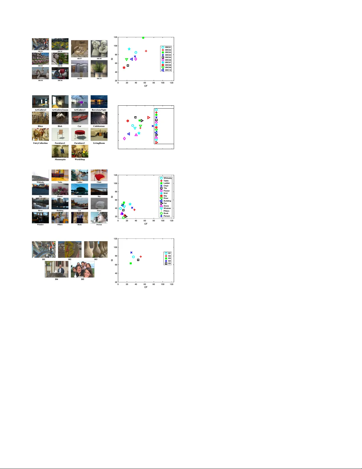
IEEE TRANSA CTIONS ON CIRCUITS AND SYSTEMS FOR VIDEO TECHNOLOGY 1 No-Reference Light Field Image Quality Assessment Based on Spatial-Angular Measurement Likun Shi, W ei Zhou, Student Member , IEEE , Zhibo Chen, Senior Member , IEEE , and Jinglin Zhang Abstract —Light field image quality assessment (LFI-QA) is a significant and challenging resear ch problem. It helps to better guide light field acquisition, processing and applications. Howev er , only a few objective models have been proposed and none of them completely consider intrinsic factors affecting the LFI quality . In this paper , we propose a No-Refer ence Light Field image Quality Assessment (NR-LFQA) scheme, where the main idea is to quantify the LFI quality degradation through evaluating the spatial quality and angular consistency . W e first measure the spatial quality deterioration by capturing the nat- uralness distrib ution of the light field cyclopean image array , which is formed when human observes the LFI. Then, as a transformed repr esentation of LFI, the Epipolar Plane Image (EPI) contains the slopes of lines and in volv es the angular information. Theref ore, EPI is utilized to extract the global and local features fr om LFI to measure angular consistency degradation. Specifically , the di stribution of gradient direction map of EPI is proposed to measure the global angular consistency distortion in the LFI. W e further pr opose the weighted local binary patter n to captur e the characteristics of local angular consistency degradation. Extensive experimental results on f our publicly available LFI quality datasets demonstrate that the proposed method outperf orms state-of-the-art 2D, 3D, multi-view , and LFI quality assessment algorithms. Index T erms —Light field image, quality assessment, epipolar plane image, naturalness, spatial quality , angular consistency . I . I N T R O D U C T I O N W ITH the rapid de velopment of acquisition, transmission and display technologies, many new media modalities (e.g. virtual reality and light field) hav e been created to provide end-users with better immersiv e viewing experiences [1], [2]. Unlike traditional media technologies, such as 2D image or stereoscopic image, light field content contains a large amount of information, which not only records radiation intensity information, but also records the direction information of light rays in the free space. Due to abundance of spatial and angular information, LF research has attracted widespread attention and has many applications, such as rendering new vie ws, depth estimation, refocusing and 3D modeling [3]. L. Shi, W . Zhou and Z. Chen are with the CAS Key Laboratory of T echnology in Geo-Spatial Information Processing and Application Sys- tem, Univ ersity of Science and T echnology of China, Hefei 230027, China, (e-mail: slikun@mail.ustc.edu.cn; weichou@mail.ustc.edu.cn; chen- zhibo@ustc.edu.cn). J. Zhang is with Key Laboratory of Meteorological Disaster , Ministry of Education, Nanjing University of Information Science and T echnology , Nanjing 210044, China, (e-mail: jinglin.zhang@nuist.edu.cn). Likun Shi and W ei Zhou contributed equally to this paper . Corresponding Authors: Zhibo Chen, Jinglin Zhang. This work was supported in part by NSFC under Grant 61571413, 61632001. Distribution of light rays is first described by Gershun et al. in 1939 [4], and then Adelson and Bergen refined its definition and explicitly defined the model called plenoptic function in 1991, which describes the light rays as a function of intensity , location in space, trav el direction, wa velength, and time [5]. Howe ver , obtaining and dealing with this multidimensional function is a huge challenge. T o solv e this problem and for practical usage, the measurement function is assumed to be monochromatic, time-inv ariant and the ray radiation remains constant along the line. The light field model can be simplified to a 4D function that can be parameterized as L ( u, v, s, t ) , where ( u, v ) represents angular coordinate and ( s, t ) expresses the spatial coordinate [6], [7]. Fig. 1 illustrates a light field image captured by L ytro Illum [8], where each image in the LFI is called a Sub-Aperture Image (SAI). Additionally , we can produce EPI by fixing a spatial coordinate ( s or t ) and an angular coordinate ( u or v ). Specifically , vertical EPI can be obtained by fixing u and s , similarly fixing v and t to get the horizontal EPI, as shown in the bottom and right of Fig. 1. According to the abov e mentioned light field function, many light field capture equipments ha ve been designed, and some of them ha ve entered the market. In general, light field acquisition approaches can be cate gorized into High Density Camera Array (HDCA), T ime-Sequential Capture (TSC) and Micro- Lens Array (MLA) [3]. Specifically , the HDCA [9] establishes an array of image sensors distributed on a plane or sphere to simultaneously capture light field samples from dif ferent viewpoints [6]. The angular dimensions are determined by the number of cameras and their distrib ution, while the spatial dimensions are determined by camera sensor . The TSC system is designed that only uses a single image sensor to capture mul- tiple samples of light field through multiple exposures, which captures light field at different vie wpoints by mo ving the image sensor [10] or fixing the camera when moving objects [11]. The angular dimensions are determined by the number of exposures, while the spatial dimensions are determined by camera sensor . In some cases (e.g. negligible illumination changes), the LFI captured by the TSC can be considered to be the same as that captured by the HDCA. Different from the structure of the above devices, the MLA (also called lenslet array) system encodes 4D LFIs into a 2D sensor plane and has been successfully commercialized [8], [12]. Fig. 2(a) exhibits the output of the L ytro Illum camera, which is called lenslet image and consists of many micro-images produced by the micro-lens (as sho wn in Fig. 2(b)). Moreo ver , the lenslet image can be further con verted into multiple SAIs, as shown in Fig. 1. The spatial resolution is defined by the number of micro- lens, and the number of pixels behind a micro-lens defines the IEEE TRANSA CTIONS ON CIRCUITS AND SYSTEMS FOR VIDEO TECHNOLOGY 2 Fig. 1: Light field image captured by L ytro Illum with the corresponding horizontal and vertical epipolar plane image. angular resolution. Benefiting from the development of the aforementioned acquisition equipment and the f ast ev aluation of 5G tech- nologies, we can foresee the explosion of immersiv e media applications presented to end-customers. Specifically , light field display architectures are generally classified into three categories: traditional light field displays [13], multilayer light field displays [14] and compressi ve light field displays [15]. Moreov er , light field images can be visualized in two w ays, namely integral light field structure (i.e. 2D array of images) and 2D slices, such as the EPI. W ith a sufficiently dense set of cameras, one can create virtual renderings of light field at any position of the sphere surf ace or ev en closer to the object by resampling and interpolating light rays [6], rather than synthesizing the vie w based on geometry information [16]. The light field quality monitoring plays an important role in the processing and applications of the LFI for pro viding users with a good viewing e xperience. Ho wev er, most LFI processing and applications do not consider specific characteristic of LFI or only utilize traditional 2D image quality assessment (IQA) metrics, which ignore the relationship between different SAIs. Existing research indicates that LFI quality is af fected by three factors, namely spatio-angular resolution, spatial quality , and angular consistency [3], [17]. The spatio-angular resolu- tion refers to the number of SAIs in a LFI and the resolution of a SAI. Moreover , the spatial quality indicates SAI quality , while the angular consistency measures the visual coherence between SAIs. Since spatio-angular resolution is determined by acquisition devices, this paper focuses on the effects of spatial quality and angular consistency . In order to assess the perceptual LFI quality , we need to conduct subjectiv e experiments or build objecti ve quality assessment models. Although subjective ev aluation is the most reliable method for measuring LFI quality , it is resource and time consuming and cannot be integrated into the automatic optimization of LFI processing. Therefore, an effecti ve objec- tiv e LFI quality assessment model is necessary . Generally , according to the av ailability of original reference information, objecti ve IQA algorithms can be classified as full- (a) (b) Fig. 2: Lenslet image captured by L ytro Illum. (a) Lenslet image; (b) Amplified regions for the red bounding box of (a). reference IQA (FR-IQA), reduced-reference IQA (RR-IQA), and no-reference IQA (NR-IQA). Specifically , the FR-IQA methods utilize complete reference image data and measure the dif ference between reference and distorted images. The RR-IQA models utilize partial information of the reference image for quality assessment, while the NR-IQA metrics e val- uate image quality without original reference images, which is more applicable in most real-world scenarios. For 2D IQA, several 2D FR-IQA metrics have been pro- posed, for example, structural similarity (SSIM) [18], multi- scale SSIM (MS-SSIM) [19], feature similarity (FSIM) [20], information content weighting SSIM (IWSSIM) [21], internal generativ e mechanism (IGM) [22], visual saliency-induced index (VSI) [23] and gradient magnitude similarity deviation (GMSD) [24]. The degree of information loss for the distorted image relativ e to the reference image is ev aluated in informa- tion fidelity criterion (IFC) [25] and visual information fidelity (VIF) [26]. The noise quality measure (NQM) [27] and visual signal-to-noise ratio (VSNR) [28] consider the human visual system (HVS) sensiti vity to dif ferent visual signals and the interaction between different signal components. Moreo ver , there also e xist some 2D RR-IQA metrics, such as [29]– [31], and 2D NR-IQA metrics. The distortion identification- based image verity and integrity e v aluation (DIIVINE) mon- itors natural image behaviors based on scene statistics [32]. The generalized Gaussian density function is modeled by block discrete cosine transform (DCT) coefficients in blind image integrity notator using DCT statistics (BLIINDS-II) [33]. The blind/referenceless image spatial quality ev aluator (BRISQUE) utilizes scene statistics from spatial domain [34]. The natural image quality e v aluator (NIQE) extracts image local features and fits a multi v ariate Gaussian model on the extracted local features [35]. A “bag” of features designed in different color spaces based on human perception are extracted in feature maps-based referenceless image quality e v aluation engine (FRIQUEE) [36]. In addition, due to the high dynamic properties of light field content, we also compare with the visual difference predictor for high dynamic range images (HDR-VDP2) [37]. As for 3D IQA, Y ang et al. proposed a 3D FR-IQA method based on the av erage peak signal-to-noise ratio (PSNR) and the absolute dif ference between left and right vie ws [38]. Chen et al. proposed a 3D FR-IQA algorithm that models the influence of binocular riv alry [39]. They also proposed a IEEE TRANSA CTIONS ON CIRCUITS AND SYSTEMS FOR VIDEO TECHNOLOGY 3 (a) 0 20 40 60 80 100 120 CF 20 40 60 80 100 120 SI SRC01 SRC02 SRC03 SRC04 SRC05 SRC06 SRC07 SRC08 SRC09 SRC10 (b) (c) 0 20 40 60 80 100 120 CF 20 40 60 80 100 120 SI ArtGallery2 ArtGallery2zoom ArtGallery3 BarcelonaNight Bikes Blob Car Cobblestone FairyCollection Furniture1 Furniture3 LivingRoom Mannequin WorkShop (d) (e) 0 20 40 60 80 100 120 CF 20 40 60 80 100 120 SI Whitesky Table Ladder Chair Tile Flower Grid Sky River Building Car Stone Window Pillars Book Person (f) (g) 0 20 40 60 80 100 120 CF 20 40 60 80 100 120 SI I01 I02 I03 I04 I05 (h) Fig. 3: (a) Illustration of the center view for the selected image contents of source sequences of W in5-LID; (b) Distribution of Spatial perceptual Information (SI) and Colorfulness (CF) of W in5-LID; (c) Illustration of the center view for the selected image contents of source sequences of MPI-LF A; (d) Distribution of SI and CF of MPI-LF A; (e) Illustration of the center vie w for the selected image contents of source sequences of SMAR T ; (f) Distribution of SI and CF of SMAR T ; (g) Illustration of the center view for the selected image contents of source sequences of V ALID; (h) Distribution of SI and CF of V ALID. 3D NR-IQA algorithm that e xtracts features from cyclopean images, disparity maps, and uncertainty maps [40]. The S3D integrated quality (SINQ) considers the impact of binocular fusion, ri v alry , suppression, and a re verse salienc y ef fect on the distortion perception [41]. The depth information and binocular vision theory are utilized in (BSVQE) [42]. Regarding to multi-vie w IQA, the morphological p yramid PSNR (MP-PSNR) Full [43] and MP-PSNR Reduc [44] were proposed. Furthermore, morphological wav elet PSNR (MW - PSNR) adopts morphological wa velet decomposition to ev al- uate multi-view image quality [45]. The 3D synthesized vie w image quality metric (3DSwIM) is based on the comparison of statistical features extracted from wav elet subbands for origi- nal and distorted multi-view images [46]. Gu et al. proposed a NR multi-view IQA metric that employs the autoregression based local image description, which is named as AR-plus thresholding (APT) [47]. Howe ver , the abov e-mentioned algorithms do not take into account the essential characteristics of the LFI. Specifically , the 2D and 3D algorithms ignore the influence of angular consistency , and the multi-vie w methods cannot ef fectiv ely measure the deterioration of spatial quality . Therefore, it is important to design an effecti ve light-field-specific metric. Although there exist the ev aluation methods for light field rendering and visualization [48], [49], few objective LFI quality ev aluation methods have been proposed. Specifically , Fang et al. proposed a FR LFI-QA method that measures the gradient magnitude similarity of reference and distorted EPIs [50]. The RR LF image quality assessment metric (LF- IQM) assumes that depth map quality is closely related to LFIs overall quality , which measures the structural similarity between original and distorted depth maps to predict the LFI quality [51]. Ho we ver , neither of these methods utilize te xture information of SAI, which causes insufficient measurement of LFI spatial quality . Furthermore, LF-IQM performance is sig- nificantly affected by depth estimation algorithms. Addition- ally , these methods require the use of original LFI information, which limits their application scenarios. Therefore, a general- purpose NR LFI-QA method that fully considers the factors affecting LFI quality is necessary for real applications. In this paper , to the best of our knowledge, we propose the first No-Reference Light Field image Quality Assessment (NR-LFQA) scheme. As the LFI can provide the binocular cue and consists of many SAIs [52], we propose Light field Cyclopean image array Naturalness (LCN) to measure the deterioration of spatial quality in LFI, which can tak e advantage of information from all SAIs and effecti vely capture the global naturalness distribution of LFI. Specifically , we first mimic binocular fusion and riv alry to generate Light Field Cyclopean Image Array (LFCIA) and then analyze its naturalness distribution. In addition to spatial quality , angular consistency is equally important for the LFI perception [52], [53]. Since the EPI contain angle information of the LFI, we extract features for measuring the degradation of angular consistency on EPI including two ke y aspects: i) we propose the ne w Gradient Direction Distrib ution (GDD) to measure the distribution of EPI gradient direction maps, which can represent the global angular distribution; ii) we then propose the W eighted Local Binary Pattern (WLBP) descriptor to capture the relationship between different SAIs, which focuses on the local angular consistenc y de gradation. Finally , these two features can collecti vely reflect changes in angular consistency . Our experimental results show that the performance of our proposed NR-LFQA model correlates well with human visual perception and achieves the state-of-the-art performance com- IEEE TRANSA CTIONS ON CIRCUITS AND SYSTEMS FOR VIDEO TECHNOLOGY 4 Fig. 4: Flow diagram of the proposed No-Reference Light Field image Quality Assessment (NR-LFQA) model. pared to other objectiv e methods. The software release of NR- LFQA is av ailable online: http://staff.ustc.edu.cn/ ∼ chenzhibo/ resources.html for public research usage. The remainder of this paper is organized as follo ws. Section II introduces adopted datasets in details. In Section IIII, the proposed model is presented. W e then illustrate the experi- mental results in Section IV . Finally , section V concludes our paper . I I . D A T A S E T S W e conducted experiments on four publicly av ailable datasets, namely W in5-LID [52], MPI-LF A [53], SMAR T [54] and V ALID [55] to examine our proposed NR-LFQA model. The W in5-LID dataset selects 6 real scenes captured by L ytro illum and 4 synthetic scenes as original images, which cov er v arious Spatial perceptual Information (SI) and Col- orfulness (CF) [56], as shown in Fig. 3. The 220 distorted LFIs were produced by 6 distortion types, including HEVC, JPEG2000 (JPEG), linear interpolation (LN), nearest neighbor interpolation (NN) and two CNN models. In addition to CNN models, each distortion includes 5 intensity le vels. The observers were asked to rate 220 LFIs under double-stimulus continuous quality scale (DSCQS) on a 5-point discrete scale. The associated o verall mean opinion score (MOS) v alue is provided for each LFI. As shown in Fig. 3, the MPI-LF A dataset is composed of 14 pristine LFIs captured by the TSC system, covering v arious SI and CF . Moreover , 336 distorted LFIs were produced based on 6 distortion types (i.e. HEVC, DQ, OPT , LINEAR, NN and GA USS), with 7 degradation lev els for each distortion type. T o quantify LFI quality , pair-wise comparison (PC) method with a two-alternativ e-forced-choice is performed and just- objectionable-differences (JOD) is provided, which is more similar to dif ference-mean-opinion-score (DMOS). The lower value indicates the worse quality . The SMAR T dataset contains 16 original light field images and 256 distorted sequences are obtained by introducing 4 compression distortions (i.e. HEVC intra, JPEG, JPEG2000 and SSDC). The PC method is selected to collect the subjecti ve ratings for each image and the Bradley-T erry (BT) scores are provided. Higher BT score indicates higher preference rate. The V ALID dataset consists of 5 reference LFIs with 140 distorted LFIs spanning 5 compression solutions. The V ALID includes both 8bit and 10bit LFIs. The comparison-based adjectiv al categorical judgement methodology is adopted for 8bit images, while double stimulus impairment scale (DSIS) is performed for 10bit images. Moreov er , the MOS v alues are provided for the LFIs. I I I . P R O P O S E D M E T H O D The block diagram of the proposed model is shown in Fig. 4. First, we analyze the naturalness distribution of LFCIA, which is generated by simulating binocular fusion and binocular riv alry . T o measure the degradation of angular consistency , GDD is then computed to analyze the direction distribution of EPI gradient direction maps. The WLBP descriptor is proposed to measure the relationship between different SAIs. Finally , regression model is used to predict LFI quality . A. Light field Cyclopean image array Naturalness (LCN) In general, as the LFI perceptual quality is decided by the HVS, it is reasonable to quantify the LFI quality by characterizing the human perception process. Considering that the LFI can pro vide binocular perception, we utilize the binocular fusion and binocular ri valry theory to ev aluate the spatial quality of LFI. In specific, the disparity between the left and right vie ws of the LFI is small, so most scenes are guaranteed in the comfort zone and binocular fusion occurs [57]. When the perceived contents to the left and right e yes are significantly different, the failures of binocular fusion will lead to binocular riv alry [58]. T o simulate the human perception process, the cyclopean perception theory pro vides us with an executable strategy to achieve this goal [59]. When a stereoscopic image pair is presented, a cyclopean image is formed in the mind of observers. The generated cyclopean image contains both left and right vie w information and takes into account the impact of binocular fusion and binocular ri v alry characteristics, so it can effecti vely reflect the percei ved image quality [39], [41]. Specifically , a cyclopean image is synthesized from the stereoscopic image, disparity map, and spatial acti vity map. Here, the horizontal adjacent SAIs of the LFI are regraded as a IEEE TRANSA CTIONS ON CIRCUITS AND SYSTEMS FOR VIDEO TECHNOLOGY 5 (a) (b) (c) Fig. 5: Statistical distribution of Light Field Cyclopean Image Array (LFCIA) and Mean Subtracted and Contrast Normalized (MSCN) coefficients. (a) Statistical distribution of LFCIA; (b) MSCN coefficients of LFCIA; (c) MSCN coefficients for different HEVC compression lev els. left vie w and a right vie w separately . W e define the left view as I u,v ( s, t ) , where ( s, t ) represents the SAI spatial coordinates and ( u, v ) ∈ { U, V } indicates the angular coordinate of the LFI. The LFCIA with angular resolution of U × ( V − 1) can be synthesized by the following model: C u,v ( s, t ) = W u,v ( s, t ) × I u,v ( s, t )+ W u +1 ,v ( s, t ) × I u +1 ,v (( s, t ) + d s,t ) , (1) where C u,v represents a sub-cyclopean image at angular coordinate ( u, v ) and d s,t is the horizontal disparity between I u,v and I u +1 ,v at spatial coordinate ( s, t ) . The disparity map d is generated by using a simple stereo disparity estimation algorithm, which utilizes the SSIM index as a matching criterion [39]. The weights W u,v and W u +1 ,v are computed by the following formulas: W u,v ( s, t ) = ε [ S u,v ( s, t )] + A 1 ε [ S u,v ( s, t )] + ε [ S u +1 ,v (( s, t ) + d s,t )] + A 1 , (2) W u +1 ,v ( s, t ) = ε [ S u +1 ,v (( s, t ) + d s,t )] + A 1 ε [ S u,v ( s, t )] + ε [ S u,v +1 (( s, t ) + d s,t )] + A 1 , (3) where A 1 is the small v alue to guarantee stability . S u,v ( s, t ) is N × N region pixels centered on ( s, t ) and ε [ S u,v ( s, t )] is the spatial acti vity within S u,v ( s, t ) . W e then obtain the spatial activity map as follows: ε [ S u,v ( s, t )] = log 2 [ v ar 2 u,v ( s, t ) + A 2 ] , (4) where v ar u,v ( s, t ) is the v ariance of S u,v ( s, t ) and unit item A 2 guarantee the activity is positive. Similarly , we define quantities S u +1 ,v ( s, t ) , v ar u +1 ,v ( s, t ) and ε [ S u +1 ,v ( s, t )] on the I u +1 ,v ( s, t ) . After obtaining the LFCIA, the locally Mean Subtracted and Contrast Normalized (MSCN) coefficients are utilized to measure their naturalness, which ha ve been successfully employed for image processing tasks and can be used to model the contrast-gain masking process in early human vision [34], [60]. F or each sub-cyclopean image, its MSCN coefficients can be calculated by: b C u,v ( s, t ) = C u,v ( s, t ) − µ u,v ( s, t ) σ u,v ( s, t ) + 1 , (5) where b C u,v ( s, t ) and C u,v ( s, t ) represent the MSCN coef- ficients image and sub-cyclopean image v alues at spatial position ( s, t ) respecti vely . µ u,v ( s, t ) and σ u,v ( s, t ) stands for the local mean and standard de viation in a local patch centered at ( s, t ) . They are respectiv ely calculated as: µ u,v ( s, t ) = K X k = − K L X l = − L z k,l C k,l u,v ( s, t ) , (6) σ u,v ( s, t ) = v u u t K X k = − K L X l = − L z k,l ( C k,l u,v ( s, t ) − µ u,v ( s, t )) 2 , (7) where z = { z k,l | k = − K, ..., K , l = − L, ..., L } denotes a 2D circularly-symmetric gaussian weighting function sampled out 3 standard deviations and rescaled to unit volume. W e set K = L = 3 in our implement. T o measure the spatial quality of the LFI, we consider the naturalness distribution of LFCIA. In specific, the MSCN coefficients of all sub-cyclopean images are superimposed. As shown in Fig. 5(a) and Fig. 5(b), the distribution of MSCN coefficients is significantly different from the statistical distribution of sub-cyclopean images and approximates the Gaussian distribution. Fig. 5(c) illustrates the MSCN coef- ficients distributions of LFIs with dif ferent high efficiency video coding (HEVC) compression levels, the results of which represent that the MSCN coefficients distributions are very indicativ e when the LFI suffer from distortions. Here the sample of LFI is selected from the W in5-LID dataset [52]. Then, we utilize the zero-mean asymmetric generalized gaus- sian distribution (A GGD) model to qualify MSCN coefficients distribution, which can fit the distribution by: f ( x ; α, σ 2 l , σ 2 r ) =        α ( β l + β r )Γ( 1 α ) exp ( − ( − x β l ) α ) x < 0 α ( β l + β r )Γ( 1 α ) exp ( − ( − x β r ) α ) x > 0 , (8) IEEE TRANSA CTIONS ON CIRCUITS AND SYSTEMS FOR VIDEO TECHNOLOGY 6 Fig. 6: Horizontal EPI for a undistorted LFI and its various distorted versions. The samples are selected from the MPI-LFI dataset [53]. (a-b) Center view of the LFIs and the red line indicates the row position at which the EPI is acquired; (c-d) Original EPIs; (e-f) Distorted EPIs with LINEAR distortion; (g-h) Distorted EPIs with NN distortion. Fig. 7: Gradient direction distribution for a undistorted LFI and its various distorted types. where β l = σ l s Γ( 1 α ) Γ( 3 α ) and β r = σ r s Γ( 1 α ) Γ( 3 α ) , (9) and α is the shape parameter controlling the shape of the statistic distrib ution, while σ l , σ r are the scale parameters of the left and right sides respecti vely . If σ l = σ r , AGGD can become generalized gaussian distribution (GGD) model. In addition, we utilize aforementioned three parameters to compute η as another feature: η = ( β r − β l ) Γ( 2 α ) Γ( 1 α ) . (10) W e further compute kurtosis and ske wness as supplementary features. In addition, the SAIs are downsampled by a factor of 2, which has been prov en to improve the correlation between model prediction and subjectiv e assessment [34]. Finally , LFCIA naturalness F LC N is obtained. B. Global Direction Distribution (GDD) The LFI quality is af fected by spatial quality and angular consistency . Usually , angular reconstruction operations, such as interpolation, will break angular consistency . T o measure the deterioration of angular consistency , e xtracting features from the EPI is an executable strategy because it contains the angular information of the LFI. T raditionally , the slopes of lines in the EPI reflect the depth of the scene captured by light field. Man y LFI processing tasks, such as super resolution and depth map estimation, benefit from this particular property [3], [61]. As sho wn in Fig. 6(c-d), the slopes of lines in the undistorted EPI can effecti vely reflect the depth and disparity information in Fig. 6(a-b). Here the LFIs are from MPI-LF A dataset [53]. Howe ver , angular distortion damages existing structures and significantly changes the distribution of the slopes of lines in the EPI, as presented in Fig. 6(e-h). Specifically , we find that the distorted EPIs with the same distortion type hav e a similar distribution, indicating that the angular distortion is not sensitiv e to the depth and content of the original LFI. Therefore, the slopes of lines in distorted EPI can be utilized to capture the degradation of angular distortion of LFI. T o extract the Gradient Direction Distrib ution (GDD) fea- tures, we first compute the gradient direction maps of EPIs and then analyze the distribution of the gradient direction maps to obtain the features. W e define the vertical EPI and horizontal EPI as E u ∗ ,s ∗ ( v , t ) and E v ∗ ,t ∗ ( u, s ) respectiv ely , where u ∗ , s ∗ and v ∗ , t ∗ represent the fixed coordinates. Then we analyze the direction distrib ution of EPI by calculating the gradient direction maps of EPI: G u ∗ ,s ∗ = atan 2( − E y u ∗ ,s ∗ , E x u ∗ ,s ∗ ) ∗ 180 π , (11) where E x u ∗ ,s ∗ = E u ∗ ,s ∗ ⊗ h x and E y u ∗ ,s ∗ = E u ∗ ,s ∗ ⊗ h y , (12) h x =   − 1 0 1 − 2 0 2 − 1 0 1   , h y =   − 1 − 2 − 1 0 0 0 1 2 1   . (13) Similar to the computation process of G u ∗ ,s ∗ , we can obtain the gradient direction maps G v ∗ ,t ∗ of horizontal EPI. W e then quantify the gradient direction maps to 360 bins, i.e. from − 180 ◦ to 179 ◦ . As shown in Fig. 7, v arious distortion types exert systematically dif ferent influences on the EPIs. It can be seen that the original EPI has a direction histogram concentrated on about − 150 ◦ and 30 ◦ , while the distorted EPIs manifest different distributions. Specifically , the nearest neighbor (NN) and LINEAR interpolation distortions make the EPIs appear stepped, and their direction is mainly concentrated at − 180 ◦ and 0 ◦ . The optical flo w estimation (OPT) and quantized depth maps (DQ) distortions sho w higher peaks at − 150 ◦ and 30 ◦ . Overall, gradient direction distrib ution is effecti ve for measuring the degradation of angular consistency . IEEE TRANSA CTIONS ON CIRCUITS AND SYSTEMS FOR VIDEO TECHNOLOGY 7 (a) (b) (c) (d) Fig. 8: Illustration of the statistical distribution of WLBP with different distortion types from MPI-LF A [53]. Here we set R = 1 and P = 8 . (a) Quantized depth maps (DQ). (b) Optical flow estimation (OPT). (c) LINEAR interpolation. (d) Nearest Neighbor (NN) interpolation. (a) (b) (c) (d) Fig. 9: Illustration of the statistical distribution of WLBP with different NN distortion levels from MPI-LF A [53]. Here we set R = 1 and P = 8 . (a) Level 1; (b) Lev el 2; (c) Le vel 3; (d) Level 4. Finally , we calculate the mean value, entrop y , skewness and kurtosis of the G u ∗ ,s ∗ and G v ∗ ,t ∗ , respectively . Since the LFI contains many EPIs, we av erage the mean v alue, entropy , ske wness and kurtosis of all EPIs to obtain the feature F GDD . C. W eighted Local Binary P attern (WLBP) Since the pixels in each row of the EPI come from dif ferent SAIs, the relationship between the pixels of each row can reflect the relationship of the SAIs. This property indicates that we can analyze the relati ve relationship of pixels in EPI to measure the change in angular consistency . In addtion, mea- suring the relationship between pix els at different distances can capture local angular consistency information. As a result, we propose W eighted Local Binary P attern (WLBP) to capture the relationship between dif ferent SAIs. The LBP is able to extract local distribution information, which has prov en its effecti veness in many works and has shown good performance for the e v aluation of 2D-IQA tasks [62]–[67]. W e first calculate the local rotation in v ariant uni- form LBP operator L R,P u ∗ ,s ∗ of the vertical EPI E u ∗ ,s ∗ by: L R,P u ∗ ,s ∗ ( E c u ∗ ,s ∗ ) =        P − 1 X p =0 θ ( E p u ∗ ,s ∗ − E c u ∗ ,s ∗ ) ψ ( ˆ L R,P u ∗ ,s ∗ ) ≤ 2 P + 1 otherw ise, (14) where R is the radius value and P indicates the number of neighboring points. E c u ∗ ,s ∗ represents a center pixel at the position ( x c , y c ) in the corresponding EPIs and E p u ∗ ,s ∗ is a neighboring pixel ( x p , y p ) surrounding E c u ∗ ,s ∗ : x p = x c + R cos(2 π p P ) and y p = y c − R sin(2 π p P ) , (15) where p ∈ { 1 , 2 ...P } is the number of neighboring pixels sampled by a distance R from E c u ∗ ,s ∗ to E p u ∗ ,s ∗ . In this case, θ ( z ) is the step function and defined by: θ ( z ) = ( 1 z > T 0 other w ise, (16) where T indicates the threshold value. In addition, ψ is used to compute the number of bitwise transitions: ψ ( L R,P u ∗ ,s ∗ ) = || θ ( E P − 1 u ∗ ,s ∗ − E c u ∗ ,s ∗ ) − θ ( E 0 u ∗ ,s ∗ − E c u ∗ ,s ∗ ) || + P − 1 X p =1 || θ ( E p u ∗ ,s ∗ − E c u ∗ ,s ∗ ) − θ ( E p − 1 u ∗ ,s ∗ − E c u ∗ ,s ∗ ) || , (17) and ˆ L R,P u ∗ ,s ∗ is rotation-in variant operator: ˆ L R,P u ∗ ,s ∗ ( E c u ∗ ,s ∗ ) = min { ROR ( P − 1 X p =0 θ ( E p u ∗ ,s ∗ − E c u ∗ ,s ∗ )2 p , k ) } , (18) where k ∈ { 0 , 1 , 2 ..., P − 1 } and RO R ( β , k ) is the circular bit-wise right shift operator that shifts the tuple β by k positions. Finally , we obtain L R,P u ∗ ,s ∗ with a length of P + 2 . For a LFI, there exist many EPIs in the vertical and horizon- tal directions. If we concatenate the LBP features that e xtracted from each EPI, it will induce a dimensional disaster . T o reduce the feature dimension, entropy weighting is adopted because some EPIs hav e little information and their LBP features are mainly concentrated in one statistical direction. This represents that these EPIs contain less angular consistency information IEEE TRANSA CTIONS ON CIRCUITS AND SYSTEMS FOR VIDEO TECHNOLOGY 8 T ABLE I: Performance Comparison on Win5-LID, MPI-LF A, and SMAR T Datasets. Win5-LID MPI-LF A SMAR T T ype Metrics SRCC LCC RMSE OR SRCC LCC RMSE OR SRCC LCC RMSE OR 2D FR PSNR 0.6026 0.6189 0.8031 0.0045 0.8078 0.7830 1.2697 0.0060 0.7045 0.7035 1.5330 0.0195 SSIM [18] 0.7346 0.7596 0.6650 0.0000 0.7027 0.7123 1.4327 0.0060 0.6862 0.7455 1.4378 0.0156 MS-SSIM [19] 0.8266 0.8388 0.5566 0.0000 0.7675 0.7518 1.3461 0.0060 0.6906 0.7539 1.4171 0.0117 FSIM [20] 0.8233 0.8318 0.5675 0.0045 0.7776 0.7679 1.3075 0.0030 0.7811 0.8139 1.2533 0.0039 IWSSIM [21] 0.8352 0.8435 0.5492 0.0000 0.8124 0.7966 1.2340 0.0030 0.7111 0.7971 1.3024 0.0000 IFC [25] 0.5028 0.5393 0.8611 0.0000 0.7573 0.7445 1.3629 0.0030 0.4827 0.5946 1.7343 0.0156 VIF [26] 0.6665 0.7032 0.7270 0.0000 0.7843 0.7861 1.2618 0.0030 0.0684 0.2533 2.0867 0.0469 NQM [27] 0.6508 0.6940 0.7362 0.0045 0.7202 0.7361 1.3817 0.0060 0.4601 0.5305 1.8285 0.0234 VSNR [28] 0.3961 0.5050 0.8826 0.0182 0.7427 0.5787 1.6651 0.0179 0.5542 0.6289 1.6770 0.0156 HDR-VDP2 [37] 0.5555 0.6300 0.7941 0.0045 0.8608 0.8385 1.1123 0.0000 0.1888 0.3347 2.0327 0.0625 2D NR BRISQUE [34] 0.6687 0.7510 0.5619 0.0000 0.6724 0.7597 1.1317 0.0000 0.8239 0.8843 0.8325 0.0000 NIQE [35] 0.2086 0.2645 0.9861 0.0045 0.0665 0.1950 2.0022 0.0327 0.1386 0.1114 2.1436 0.0547 FRIQUEE [36] 0.6328 0.7213 0.5767 0.0000 0.6454 0.7451 1.1036 0.0000 0.7269 0.8345 0.9742 0.0000 3D FR Chen [39] 0.5269 0.6070 0.8126 0.0091 0.7668 0.7585 1.3303 0.0030 0.6798 0.7722 1.3706 0.0078 3D NR SINQ [41] 0.8029 0.8362 0.5124 0.0000 0.8524 0.8612 0.9939 0.0000 0.8682 0.8968 0.9653 0.0000 BSVQE [42] 0.8179 0.8425 0.4801 0.0000 0.8570 0.8751 0.9561 0.0000 0.8449 0.8992 0.8514 0.0000 Multi-view FR MP-PSNR Full [43] 0.5335 0.4766 0.8989 0.0000 0.7203 0.6730 1.5099 0.0089 0.8449 0.8992 0.8514 0.0000 MP-PSNR Reduc [44] 0.5374 0.4765 0.8989 0.0000 0.7210 0.6747 1.5067 0.0089 0.6716 0.6926 1.5559 0.0117 MW -PSNR Full [45] 0.5147 0.4758 0.8993 0.0000 0.7232 0.6770 1.5023 0.0089 0.6620 0.6505 1.6382 0.0117 MW -PSNR Reduc [45] 0.5326 0.4766 0.8989 0.0000 0.7217 0.6757 1.5048 0.0089 0.6769 0.6903 1.5607 0.0117 3DSwIM [46] 0.4320 0.5262 0.8695 0.0182 0.5565 0.5489 1.7063 0.0119 0.4053 0.4707 1.9032 0.0234 Multi-view NR APT [47] 0.3058 0.4087 0.9332 0.0045 0.0710 0.0031 2.0413 0.0357 0.5105 0.5249 1.8361 0.0234 LFI FR Fang [50] - - - - 0.7942 0.8065 1.2300 - - - - - LFI RR LF-IQM [51] 0.4478 0.5193 0.8584 0.0227 0.3334 0.4360 1.8038 0.0149 0.1701 0.2101 1.0279 0.0392 LFI NR Pr oposed NR-LFQA 0.9032 0.9206 0.3876 0.0000 0.9119 0.9155 0.7556 0.0000 0.8803 0.9105 0.8300 0.0000 T ABLE II: Performance Comparison on V ALID Dataset. V ALID-8bit V ALID-10bit T ype Metrics SRCC LCC RMSE OR SRCC LCC RMSE OR 2D FR PSNR 0.9620 0.9681 0.3352 0.0000 0.9467 0.9524 0.2935 0.0000 SSIM [18] 0.9576 0.9573 0.3868 0.0000 0.9326 0.9375 0.3348 0.0000 MS-SSIM [19] 0.9593 0.9658 0.3473 0.0000 0.9432 0.9484 0.3051 0.0000 FSIM [20] 0.9695 0.9798 0.2678 0.0000 - - - - IWSSIM [21] 0.9674 0.9764 0.2892 0.0000 0.9499 0.9617 0.2638 0.0000 IFC [25] 0.9693 0.9909 0.1800 0.0000 - - - - VIF [26] 0.9749 0.9870 0.2150 0.0000 - - - - NQM [27] 0.9055 0.9194 0.5266 0.0000 0.8410 0.8582 0.4940 0.0000 VSNR [28] 0.9359 0.9324 0.4838 0.0000 - - - - HDR-VDP2 [37] 0.9623 0.9785 0.2758 0.0000 0.9371 0.9528 0.2921 0.0000 2D NR BRISQUE [34] 0.9222 0.9849 0.2017 0.0000 0.9027 0.9347 0.2838 0.0000 NIQE [35] 0.8636 0.9524 0.4080 0.0000 - - - - FRIQUEE [36] 0.9157 0.9836 0.2160 0.0000 0.8559 0.8986 0.3497 0.0000 3D FR Chen [39] 0.9642 0.9738 0.3046 0.0000 - - - - 3D NR SINQ [41] 0.9222 0.9849 0.2070 0.0000 0.9021 0.9348 0.2722 0.0000 BSVQE [42] 0.9222 0.9814 0.2180 0.0000 - - - - Multi-view FR MP-PSNR Full [43] 0.9730 0.9852 0.2291 0.0000 0.3830 0.3582 0.8986 0.0000 MP-PSNR Reduc [44] 0.9744 0.9859 0.2237 0.0000 0.3826 0.3506 0.9013 0.0000 MW -PSNR Full [45] 0.9597 0.9677 0.3376 0.0000 0.3764 0.3556 0.8995 0.0000 MW -PSNR Reduc [45] 0.9648 0.9751 0.2970 0.0000 0.3815 0.3563 0.8993 0.0100 3DSwIM [46] 0.7950 0.7876 0.8248 0.0000 0.7869 0.7401 0.6472 0.0000 Multi-view NR APT [47] 0.4699 0.6452 1.0228 0.0000 - - - - LFI RR LF-IQM [51] 0.3571 0.4708 1.0712 0.0000 0.3692 0.4828 0.8137 0.0000 LFI NR Pr oposed NR-LFQA 0.9286 0.9799 0.2380 0.0000 0.9228 0.9517 0.2769 0.0000 and their entropy values are close to zero. Therefore, we can obtain the WLBP of vertical EPI E u ∗ ,s ∗ as follows: Lv er R,P = U P u =1 S P s =1 w R,P u,s . ∗ L R,P u,s U P u =1 S P s =1 w R,P u,s , (19) IEEE TRANSA CTIONS ON CIRCUITS AND SYSTEMS FOR VIDEO TECHNOLOGY 9 0.84 0.86 0.88 0.9 0.92 0.94 0.96 0.98 1 FSIM 0 1 2 3 4 5 MOS (a) 0.85 0.9 0.95 1 MSSIM 0.5 1 1.5 2 2.5 3 3.5 4 4.5 5 MOS (b) 0.75 0.8 0.85 0.9 0.95 1 IWSSIM 0.5 1 1.5 2 2.5 3 3.5 4 4.5 5 MOS (c) -1 0 1 2 3 4 5 BSVQE 0.5 1 1.5 2 2.5 3 3.5 4 4.5 5 MOS (d) 0 1 2 3 4 5 Proposed Model 0.5 1 1.5 2 2.5 3 3.5 4 4.5 5 MOS (e) Fig. 10: The scatter plots of predicted quality scores by different methods against the MOS values on the W in5-LID. The horizontal axis in each figure denotes predicted quality scores and the vertical axis in each figure represents the MOS values. The red line is the fitted curve. (a) FSIM; (b) MS-SSIM; (c) IWSSIM; (d) BSVQE; (e) Proposed. PSNR SSIM VIF FSIM MSSIM IWSSIM VSNR UQI IFC NQM NIQE HDR-VDP2 BRISQUE FRIQUEE Chen SINQ BSVQE 3DSwIM MW-PSNR Reduc MW-PSNR Full MP-PSNR Reduc MP-PSNR Full APT LF-IQM NR-LFQA 0 0.2 0.4 0.6 0.8 1 SRCC (a) PSNR SSIM VIF FSIM MSSIM IWSSIM VSNR UQI IFC NQM NIQE HDR-VDP2 BRISQUE FRIQUEE Chen SINQ BSVQE 3DSwIM MW-PSNR Reduc MW-PSNR Full MP-PSNR Reduc MP-PSNR Full APT LF-IQM NR-LFQA 0 0.2 0.4 0.6 0.8 1 SRCC (b) Fig. 11: Box plot of SRCC distributions of algorithms over 1000 trials. (a) On W in5-LID dataset; (b) On MPI-LF A dataset. where the entropy of L R,P u,s is computed as weight w R,P u,s . At the same time, we adopt the same operation to obtain the WLBP features Lhor R,P of the horizontal EPI E v ∗ ,t ∗ . In our implement, we set R ∈ { 1 , 2 , 3 } , P = 3 × R and T = R/ 2 . Finally , we combine all features to obtain feature F W LB P as follows: F W LB P = { Lv er R,P , Lhor R,P } . (20) Fig. 8 illustrates the WLBP histogram of various distortion types with R = 1 and P = 8 . The LFIs are selected from MPI-LF A dataset [53]. Specifically , the WLBP features are extracted from horizontal and vertical EPIs separately . For MPI-LF A dataset, the LFIs only contain horizontal EPIs. Moreov er , for the WLBP feature with parameter ( R, P ) , we can generate P + 2 histogram bins [62]. Therefore, when P = 8 , the corresponding feature dimension is P + 2 = 10 . Furthermore, the histogram of WLBP for NN distortion with different distortion levels for R = 1 and P = 8 is shown in Fig. 9. As the figures show that there is a significant difference in the WLBP distribution for different distortion types, and the WLBP distrib ution changes significantly as the distortion lev el increases. Ov erall, WLBP can ef fecti vely capture the characteristics of local angular consistency degradation in EPI. D. Quality Evaluation In order to conduct the quality assessment, we train a regression model to map the final feature vector F F inal = { F LC N , F GDD , F W LB P } space to quality scores. In our implementation, we utilize support v ector re gression (SVR) model, which can automatically learn the weights of these features from the data distribution. In other words, the weights of these proposed features are dif ferent. Moreover , the SVR model has been applied to many image quality assessment problems [41], [42], [68] and has demonstrated its effecti ve- ness The LIBSVM package [69] is exploited to implement the SVR with a radial basis function (RBF) kernel. W e select four ev aluation criteria to measure the per- formance of objectiv e quality assessment models, namely Spearman rank-order correlation coefficient (SRCC), linear correlation coefficient (LCC), root-mean-square-error (RMSE) and outlier ratio (OR). The SRCC measures the monotonicity , while the LCC e v aluates the linear relationship between pre- dict scores and MOS values. The RMSE and OR measure the prediction accuracy and prediction consistenc y , respecti vely . The SRCC and LCC values closing to 1 represent high positiv e correlation and a lower RMSE/OR value indicates a better performance. Additionally , each dataset is randomly di vided into 80% for training and 20% for testing. W e perform 1000 iterations of cross v alidation on each dataset, and provide the median SRCC, LCC, RMSE and OR performance as the final measurement. Before computing the LCC, RMSE and OR, a non-linear function is employed by: q 0 = β 1 { 1 2 − 1 1 + exp [ β 2 ( q − β 3 )] } + β 4 q + β 5 , (21) where q is the output of a method. The parameters β 1 ··· 5 are optimized to minimize a gi ven goodness-of-fit measure. IEEE TRANSA CTIONS ON CIRCUITS AND SYSTEMS FOR VIDEO TECHNOLOGY 10 T ABLE III: Performance Comparison Between Row and Column Methods W ith T -test on Win5-LID Dataset. The Symbol ‘1’, ‘0’, or ‘-1’ Represents that the Row Method is Statistically Better , Indistinguishable, or W orse Than The Column Algorithm. Due to Space Constraints, Here W e Use the Referenced Number Instead of The Algorithm Name. PSNR [18] [26] [20] [19] [21] [28] [25] [27] [35] [34] [36] [39] [41] [42] [46] [45] [45] [44] [43] [47] [51] Proposed PSNR 0 -1 -1 -1 -1 -1 1 1 -1 1 -1 -1 1 -1 -1 1 1 1 1 1 1 1 -1 [18] 1 0 1 -1 -1 -1 1 1 1 1 1 1 1 -1 -1 1 1 1 1 1 1 1 -1 [26] 1 -1 0 -1 -1 -1 1 1 1 1 0 1 1 -1 -1 1 1 1 1 1 1 1 -1 [20] 1 1 1 0 0 -1 1 1 1 1 1 1 1 1 0 1 1 1 1 1 1 1 -1 [19] 1 1 1 0 0 -1 1 1 1 1 1 1 1 1 1 1 1 1 1 1 1 1 -1 [21] 1 1 1 1 1 0 1 1 1 1 1 1 1 1 1 1 1 1 1 1 1 1 -1 [28] -1 -1 -1 -1 -1 -1 0 -1 -1 1 -1 -1 -1 -1 -1 -1 -1 -1 -1 -1 1 -1 -1 [25] -1 -1 -1 -1 -1 -1 1 0 -1 1 -1 -1 -1 -1 -1 1 -1 -1 -1 -1 1 1 -1 [27] 1 -1 -1 -1 -1 -1 1 1 0 1 -1 1 1 -1 -1 1 1 1 1 1 1 1 -1 [35] -1 -1 -1 -1 -1 -1 -1 -1 -1 0 -1 -1 -1 -1 -1 -1 -1 -1 -1 -1 -1 -1 -1 [34] 1 -1 0 -1 -1 -1 1 1 1 1 0 1 1 -1 -1 1 1 1 1 1 1 1 -1 [36] 1 -1 -1 -1 -1 -1 1 1 -1 1 -1 0 1 -1 -1 1 1 1 1 1 1 1 -1 [39] -1 -1 -1 -1 -1 -1 1 1 -1 1 -1 -1 0 -1 -1 1 0 1 -1 0 1 1 -1 [46] 1 1 1 -1 -1 -1 1 1 1 1 1 1 1 0 -1 1 1 1 1 1 1 1 -1 [42] 1 1 1 0 -1 -1 1 1 1 1 1 1 1 1 0 1 1 1 1 1 1 1 -1 [46] -1 -1 -1 -1 -1 -1 1 -1 -1 1 -1 -1 -1 -1 -1 0 -1 -1 -1 -1 1 -1 -1 [45] -1 -1 -1 -1 -1 -1 1 1 -1 1 -1 -1 0 -1 -1 1 0 1 0 0 1 1 -1 [45] -1 -1 -1 -1 -1 -1 1 1 -1 1 -1 -1 -1 -1 -1 1 -1 0 -1 -1 1 1 -1 [44] -1 -1 -1 -1 -1 -1 1 1 -1 1 -1 -1 1 -1 -1 1 0 1 0 0 1 1 -1 [43] -1 -1 -1 -1 -1 -1 1 1 -1 1 -1 -1 0 -1 -1 1 0 1 0 0 1 1 -1 [47] -1 -1 -1 -1 -1 -1 -1 -1 -1 1 -1 -1 -1 -1 -1 -1 -1 -1 -1 -1 0 -1 -1 [51] -1 -1 -1 -1 -1 -1 1 -1 -1 1 -1 -1 -1 -1 -1 1 -1 -1 -1 -1 1 0 -1 Proposed 1 1 1 1 1 1 1 1 1 1 1 1 1 1 1 1 1 1 1 1 1 1 0 Although the prediction range of the model is different, all prediction scores can be guaranteed to be ev aluated on the same scale after logistic function fitting. T ABLE IV: Performance Comparison of Existing Algorithms on EPIs. Win5-LID MPI-LF A Metrics SRCC LCC RMSE SRCC LCC RMSE PSNR 0.7190 0.7213 0.7083 0.7198 0.6972 1.4634 FSIM [20] 0.7545 0.7780 0.6424 0.7920 0.7818 1.2730 IFC [25] 0.5323 0.5010 0.8850 0.7265 0.7394 1.3743 BRISQUE [34] 0.7727 0.8473 0.4890 0.7864 0.7850 1.0453 FRIQUEE [36] 0.6225 0.6648 0.5784 0.7523 0.7652 1.0753 Fang [50] - - - 0.7942 0.8065 1.2300 Proposed 0.8829 0.9015 0.3993 0.8905 0.8954 0.8259 T ABLE V: Performance of Three Quality Components on W in5-LID and MPI-LF A Datasets. Win5-LID MPI-LF A Featur es SRCC LCC RMSE SRCC LCC RMSE F LC N 0.7464 0.8370 0.5128 0.5806 0.6260 1.2891 F GDD 0.7431 0.7745 0.6090 0.5621 0.6205 1.1383 F W LB P 0.8528 0.8771 0.4006 0.8437 0.8573 0.8900 For OR computation, according to [70]–[72], we calculate the standard deviation of the testing set. If the dif ference between the predicted score and the subjecti ve score is more than 2 times the standard deviation, this can be defined as the outlier . Specifically , the OR represents the mapped objective scores deviating from the subjective ratings in 2 standard deviation as: O R = N P i =1 ( | s i − f i | > 2 σ i ) N , (22) where N is the size of the testing set. s i and f i denote the i -th subjecti ve score and the i -th mapped objectiv e score after the non-linear mapping, respectiv ely . σ i is the i -th standard deviation of the subjectiv e scores. E. Comparison with Other Objective Metrics In order to demonstrate the ef fecti veness of our proposed NR-LFQA model, we conduct extensi ve experiments by using existing 2D, 3D, multi-view , and LFI quality assessment algorithms. In our experiments, we utilize ten 2D-FR metrics [18]–[21], [25]–[28], [37], three 2D-NR metrics [34]–[36], one 3D-FR metric [39], two 3D-NR metrics [41], [42], fi ve multi- view FR metrics [43]–[46], one multi-view NR metric [47], one LFI FR metric [50], and one LFI RR metric (i.e. LF- IQM) [51]. For all 2D-FR, multi-view FR, LFI FR, LF-IQM, NIQE and APT algorithms, the global predicted score of LFI is obtained by av eraging scores of each SAI. W e treat the horizontal adjacent SAIs of the LFI as left and right views to test 3D IQA methods. F or the rest of the methods, we first extract features on each SAI and then average them. Finally , we predict the LFI quality according to regression methods in their papers. It should be noted that for LF-IQM, we first select the Accurate Depth Map (ADM) [73] to estimate the corresponding depth maps of original and distorted light field images. Then, we calculate the SSIM value between original and distorted depth maps as objecti ve scores. Finally , the correlation between the objectiv e scores after mapping and subjectiv e ratings can be obtained as the ultimate performance results. T ABLE I sho ws the performance comparison of objective models on W in5-LID, MPI-LF A and SMAR T datasets, where bold numbers indicate the best results. W e can find that our proposed model outperforms state-of-the-art algorithms. The existing 2D and 3D algorithms only focus on spatial quality prediction, b ut do not take into account angular consistency degradation. Although multi-view e valuation methods consider IEEE TRANSA CTIONS ON CIRCUITS AND SYSTEMS FOR VIDEO TECHNOLOGY 11 T ABLE VI: SRCC of Different Distortion T ypes on W in5-LID and MPI-LF A Datasets. Win5-LID MPI-LF A T ype Metrics HEVC JPEG LN NN HEVC DQ OPT Linear NN GAUSS 2D FR PSNR 0.8183 0.8302 0.8135 0.8734 0.9226 0.7664 0.6842 0.9090 0.8895 0.9239 SSIM [18] 0.9351 0.8390 0.8501 0.8226 0.9769 0.4468 0.5609 0.8055 0.7682 0.9800 MS-SSIM [19] 0.9731 0.8947 0.8789 0.8346 0.9791 0.7087 0.6556 0.8763 0.8775 0.9702 FSIM [20] 0.9756 0.9006 0.8876 0.8661 0.9844 0.7631 0.6969 0.8745 0.8704 0.9502 IWSSIM [21] 0.9690 0.9046 0.8851 0.8313 0.9831 0.7628 0.7336 0.9144 0.9256 0.9662 IFC [25] 0.8634 0.7299 0.6179 0.8037 0.9430 0.8462 0.7909 0.9147 0.9261 0.8852 VIF [26] 0.9627 0.8982 0.8287 0.8816 0.9818 0.7057 0.6445 0.9163 0.9048 0.9506 NQM [27] 0.8861 0.7878 0.7086 0.7214 0.9515 0.6598 0.5596 0.8444 0.9264 0.9333 VSNR [28] 0.9162 0.8861 0.0208 0.1705 0.9871 0.6082 0.6634 0.8333 0.8256 0.9462 HDR-VDP2 [37] 0.7322 0.5282 0.7912 0.8711 0.8065 0.7448 0.7953 0.8632 0.9008 0.9309 2D NR BRISQUE [34] 0.9152 0.9394 0.8268 0.2516 0.9429 0.6121 0.7059 0.7333 0.0941 0.8286 NIQE [35] 0.1332 0.2161 0.3749 0.1514 0.9186 0.0500 0.1226 0.2616 0.1457 0.1413 FRIQUEE [36] 0.8545 0.9273 0.8303 0.2727 0.9429 0.7333 0.7912 0.6364 0.1059 0.9429 3D FR Chen [39] 0.9772 0.9243 0.5455 0.5995 0.9778 0.6933 0.6608 0.8720 0.8715 0.9720 3D NR SINQ [41] 0.9394 0.9362 0.8788 0.7818 0.9429 0.8182 0.7235 0.9030 0.8412 0.8286 BSVQE [42] 0.9265 0.9273 0.8632 0.8781 0.9429 0.6485 0.7471 0.9394 0.9324 0.9429 Multi-view FR MP-PSNR Full [43] 0.8750 0.8388 0.7247 0.8591 0.9404 0.8448 0.8254 0.9267 0.9108 0.9137 MP-PSNR Reduc [44] 0.9083 0.8557 0.7238 0.8542 0.9404 0.8462 0.8193 0.9318 0.9202 0.9177 MW -PSNR Full [45] 0.8548 0.8169 0.7238 0.8464 0.9395 0.8434 0.8322 0.9347 0.9260 0.9467 MW -PSNR Reduc [45] 0.9020 0.8212 0.7206 0.8604 0.9511 0.8434 0.8227 0.9265 0.9235 0.9453 3DSwIM [46] 0.4015 0.3842 0.5455 0.7983 0.4897 0.6063 0.5721 0.7926 0.6878 0.6627 Multi-view NR APT [47] 0.2182 0.0881 0.4466 0.2855 0.3820 0.0559 0.2918 0.0381 0.1303 0.2207 LFI RR LF-IQM [51] 0.1152 0.5222 0.6848 0.6984 0.6000 0.1741 0.1736 0.3468 0.3882 0.7143 LFI NR Pr oposed NR-LFQA 0.9483 0.9423 0.8909 0.8903 0.9429 0.8545 0.8353 0.9515 0.9529 0.9429 angular interpolation distortion, the original intention of the design is to deal with the hole distortion caused by the synthe- sis, and it is not possible to ef fecti vely measure the distortions appearing in the LFI, such as compression distortion. More- ov er , spatial texture information is not in volv ed in e xisting LFI quality ev aluation algorithms, and LFI-IQM is greatly affected by depth map estimation algorithms. Therefore, their performance is poor on W in5-LID, MPI-LF A and SMAR T datasets. In addition, the W in5-LID and MPI-LF A datasets T ABLE VII: Cross V alidation Results by T raining The Proposed Model on W in5-LID and T esting on MPI-LF A. SRCC LCC RMSE Proposed NR-LFQA 0.8389 0.7653 0.4913 use different acquisition de vices, and the LFIs captured by the TSC in the MPI-LF A are close to that captured by HDCA. This demonstrates that our proposed model is suitable for various scenarios and acquisition devices. Specifically , the proposed method performs well for different content types with variety of SI and CF . Moreover , it also has good performance for rich semantic content. Apart from conducting experiments on Win5-LID, MPI- LF A and SMAR T datasets datasets, we also use V ALID dataset because it contains both 8bit and 10bit LFIs. As shown in T ABLE II, almost all FR algorithms deliv er good performance, and our proposed model is superior to all NR algorithms for all the codecs in V ALID dataset. This situation may be caused by that V ALID only uses 5 original LFIs, and their distribution is relativ ely concentrated. As shown in Fig. 3(h), the distribution intervals of CF and SI of V ALID are narro wer than other datasets. In order to show the prediction results more clearly , we illustrate the scatter plots of four methods and the proposed model on W in5-LID dataset in Fig. 10. Clearly , the points of NR-LFQA are more centralized than other existing methods and can be well fitted, which demonstrates that the predicted LFI quality scores by NR-LFQA are more consistent with subjectiv e ratings. T o further analyze the performance stability of our proposed model, we visualize the statistical significance. Specifically , we show box plots of the distribution of the SRCC values for each of 1000 experimental trials. Here, we randomly split the entire datasets into training and test sets according to the ratio of 8:2, and test the results of all methods for 1000 times. As shown in Fig. 11, compared with the existing methods, our proposed model results are more concentrated, indicating that NR-LFQA has better stability . The lower the standard de viation with higher median SRCC, the better the performance. Besides direct comparisons with numerous IQA methods, we also quantitati vely e valuate the statistical significance using the t-test [34] based on the SRCC v alues obtained from the 1000 train-test trials for these image quality methods. The null hypothesis is that the mean correlation for ro w metric is equal to mean correlation for the column metric with a confidence of 95%. Specifically , a v alue of ‘0’ indicates that the row and column metrics are statistically indistinguishable (or equiv alent), and we cannot reject the null hypothesis at the 95% confidence lev el. A value of ‘1’ represents that the row algorithm is statically superior to the column one, whereas a ‘-1’ indicates that the row metric is statistically worse than the column one. From the results on W in5-LID dataset in T ABLE III, we also pro ve that our proposed model is significantly better than all the objectiv e IQA algorithms. IEEE TRANSA CTIONS ON CIRCUITS AND SYSTEMS FOR VIDEO TECHNOLOGY 12 T ABLE VIII: Comparison of The Computation Time against SRCC, LCC, RMSE and OR Performance on W in5-LID Dataset. T ype Metrics T otal Computation Time (s) SRCC LCC RMSE OR 2D FR PSNR 0.8188 0.6026 0.6189 0.8031 0.0045 SSIM [18] 2.3068 0.7346 0.7596 0.6650 0.0000 MS-SSIM [19] 3.2937 0.8266 0.8388 0.5566 0.0000 FSIM [20] 14.4056 0.8233 0.8318 0.5675 0.0045 IWSSIM [21] 27.0113 0.8352 0.8435 0.5492 0.0000 IFC [25] 69.5933 0.5028 0.5393 0.8611 0.0000 VIF [26] 65.9176 0.6665 0.7032 0.7270 0.0000 NQM [27] 16.5390 0.6508 0.6940 0.7362 0.0045 VSNR [28] 4.0910 0.3961 0.5050 0.8826 0.0182 HDR-VDP2 [37] 115.1300 0.5555 0.6300 0.7941 0.0045 2D NR BRISQUE [34] 4.4593 0.6687 0.7510 0.5619 0.0000 NIQE [35] 8.8498 0.2086 0.2645 0.9861 0.0045 FRIQUEE [36] 2343.0336 0.6328 0.7213 0.5767 0.0000 3D FR Chen [39] 1239.3772 0.5269 0.6070 0.8126 0.0091 3D NR SINQ [41] 309.7299 0.8029 0.8362 0.5124 0.0000 BSVQE [42] 396.6745 0.8179 0.8425 0.4801 0.0000 Multi-view FR MP-PSNR Full [43] 32.2917 0.5335 0.4766 0.8989 0.0000 MP-PSNR Reduc [44] 16.2708 0.5374 0.4765 0.8989 0.0000 MW -PSNR Full [45] 1.1421 0.5147 0.4758 0.8993 0.0000 MW -PSNR Reduc [45] 1.1352 0.5326 0.4766 0.8989 0.0000 3DSwIM [46] 322.9451 0.4320 0.5262 0.8695 0.0182 Multi-view NR APT [47] 2626.8449 0.3058 0.4087 0.9332 0.0045 LFI RR LF-IQM [51] 1168.7424 0.4503 0.4763 0.8991 0.0273 LFI NR Pr oposed NR-LFQA 432.1031 0.9032 0.9206 0.3876 0.0000 F . Comparison with Other Methods based on EPI Since our proposed model uses EPI information, we verify the performance of existing algorithms on EPI for fair compar- ison. Due to the size property of EPI, some algorithms are not applicable on EPI (e.g. all 3D IQA methods). The FR metrics predict the final score by av eraging scores of all EPIs, while the NR metrics extract feature from EPIs and then average these features. T ABLE IV sho ws the results of aforementioned methods on W in5-LID and MPI-LF A datasets, which indicates that our NR-LFQA outperforms existing methods. Addition- ally , for most algorithms, using EPI information does not yield performance gains. This is because they are not specifically designed to extract information from the EPI. G. V alidity of Individual Quality Component W e explore the effecti veness of three proposed components ( F LC N , F GDD , F W LB P ). The performance values are shown in T ABLE V . W e can observ e that the F W LB P performance is the best on both W in5-LID and MPI-LF A datasets because it can capture subtle changes between SAIs from EPI. This also demonstrates that the weight of F W LB P should be higher in regression. The reason for the slightly lower performance of F LC N on the MPI-LF A dataset is that only HEVC and GA USS distortion can significantly affect the spatial quality of the LFI. Moreover , other distortions primarily affect the angular consistency of the LFI. Since F GDD is insensitiv e to small angular consistency degradation and MPI-LF A contains many angular distortions with lo w distortion lev els, it has lower performance on MPI-LF A dataset. Overall, the results demonstrate the v alidity of our proposed features and the performance is improv ed after combining features. H. Robustness Against Distortion T ypes As W in5-LID and MPI-LF A datasets consist of dif ferent distortion types, we show how our proposed model performs for each distortion type. The results are listed in T ABLE VI. It can be seen that our proposed model outperforms existing objectiv e methods for most distortion types. Specifically , our proposed model achie ves the best performance for typical reconstruction distortions. The reason is that reconstruction distortions mainly destroy angle consistency and often ha ve little effect on spatial quality . Therefore, existing models are difficult to handle such distortions. The compression distortion caused by HEVC mainly leads to spatial quality degradation. Therefore, our proposed model is not as good as the FR models. Howe ver , our model is still very competitive and has the best performance in the NR methods. Similarly , GA USS distortion also mainly af fects LFI spatial quality . The JPEG distortion in W in5-LID is introduced based on lenslet, and it af fects both LFI spatial quality and angular consistency . Our proposed model can simultaneously consider the impact of these two factors, so it is not surprising that our model has the best performance for JPEG distorted LFIs. Overall, the proposed model can achie ve the excellent performance against existing objective ev aluation schemes in volving all the distortion types. I. Model Generality and T ime Complexity Since aforementioned methods are generally trained and tested on various splits of a single dataset, it is interesting to know whether the algorithm is dataset dependent. T o verify that our proposed model does not depend on the dataset, we choose the same distortion in MPI-LF A and W in5-LID. Specifically , we trained proposed model on Win5-LID dataset, IEEE TRANSA CTIONS ON CIRCUITS AND SYSTEMS FOR VIDEO TECHNOLOGY 13 and tested it on the same distortions in MPI-LF A dataset. The results are sho wn in T ABLE VII. Ob viously , the proposed model still has good performance, which proves the generality of our proposed model. As shown in the above table, we compare the proposed NR-LFQA with state-of-the-art quality assessment algorithms regarding to time complexity on Win5-LID dataset. Besides, we also list the SRCC, LCC, RMSE and OR performance values for fair comparison. From T ABLE VIII, we can find that the proposed method is v erified to ha ve lo wer computation time compared to the LFI RR metric (i.e. LF-IQM [51]). One possible explanation is that different from traditional LFI- QA metrics, our proposed algorithm does not introduce the complex computation of depth map estimation. Generally , our proposed NR-LFQA is in the same lev el of time complexity compared with state-of-the-art 3D metrics. Moreover , the pro- posed NR-LFQA demonstrates the best SRCC, LCC, RMSE and OR performance among all schemes. I V . C O N C L U S I O N In this paper , we have presented a No-Reference Light Field image Quality Assessment (NR-LFQA) scheme. The main contributions of this work are: 1) W e propose the first no- reference metric to assess LFI overall quality by measuring the degradation of spatial quality and angular consistency . 2) T o measure LFI spatial quality , we analyze the naturalness of light field cyclopean image array . 3) Since the epipolar plane image contains v arious slopes of lines reflecting angular consistency , we propose gradient direction distribution to measure the degradation of angular consistency and weighted local binary pattern is proposed to capture the subtle angular consistency changes. 4) W e compare with state-of-the-art 2D, 3D image, multi-vie w , and LFI quality assessment methods with our NR-LFQA model. Experimental results show that our model outperforms other metrics and can handle the typical distortions of LFI. In the future, we will consider to de velop a parametric model based on the proposed features and e xtend our algo- rithm to light field video quality assessment. Additionally , no- reference light field quality assessment metrics are important for future immersive media processing chain from light field content acquisition, compression, to transmission, reconstruc- tion, and display . W e will continue to explore the proposed NR-LFQA for more potential immersive applications, e.g. utilizing NR-LFQA as a loss metric to guide the optimization of synthesizing or compressing light field images. R E F E R E N C E S [1] G. T ech, Y . Chen, K. M ¨ uller , J.-R. Ohm, A. V etro, and Y .-K. W ang, “Overvie w of the multi vie w and 3D extensions of high efficiency video coding, ” IEEE T ransactions on Cir cuits and Systems for V ideo T echnology , vol. 26, no. 1, pp. 35–49, 2016. [2] R. Mekuria, K. Blom, and P . Cesar, “Design, implementation, and ev aluation of a point cloud codec for tele-immersi ve video, ” IEEE T ransactions on Circuits and Systems for V ideo T echnology , vol. 27, no. 4, pp. 828–842, 2016. [3] G. Wu, B. Masia, A. Jarabo, Y . Zhang, L. W ang, Q. Dai, T . Chai, and Y . Liu, “Light field image processing: An overvie w , ” IEEE Journal of Selected T opics in Signal Pr ocessing , vol. 11, no. 7, pp. 926–954, 2017. [4] A. Gershun, “The light field, ” J ournal of Mathematics and Physics , vol. 18, no. 1-4, pp. 51–151, 1939. [5] E. H. Adelson and J. R. Bergen, “The plenoptic function and the elements of early vision. computational models of visual processing, ” International Journal of Computer V ision , p. 20, 1991. [6] M. Lev oy and P . Hanrahan, “Light field rendering, ” in Pr oceedings of the 23rd annual conference on Computer graphics and interactive techniques . A CM, 1996, pp. 31–42. [7] S. J. Gortler, R. Grzeszczuk, R. Szeliski, and M. F . Cohen, “The lumigraph, ” in Pr oceedings of the 23r d annual confer ence on Computer graphics and interactive techniques . ACM, 1996, pp. 43–54. [8] L ytro, http://www .lytro.com, 2017. [Online]. [9] I. J. S. 29/WG1, “JPEG Pleno call for proposals on light field coding, ” Jan. 2017. [10] J. Unger, A. W enger , T . Hawkins, A. Gardner , and P . Debev ec, “Cap- turing and rendering with incident light fields, ” UNIVERSITY OF SOUTHERN CALIFORNIA MARINA DEL REY CA INST FOR CREA TIVE , T ech. Rep., 2003. [11] R. R. T amboli, B. Appina, S. Channappayya, and S. Jana, “Super- multivie w content with high angular resolution: 3D quality assessment on horizontal-parallax lightfield display , ” Signal Pr ocessing: Image Communication , vol. 47, pp. 42–55, 2016. [12] ¯ A. Raytrix, “3D light field camera technology , ” 2017. [13] B. Masia, G. W etzstein, P . Didyk, and D. Gutierrez, “ A surve y on computational displays: Pushing the boundaries of optics, computation, and perception, ” Computers & Graphics , v ol. 37, no. 8, pp. 1012–1038, 2013. [14] R. Narain, R. A. Albert, A. Bulbul, G. J. W ard, M. S. Banks, and J. F . O’Brien, “Optimal presentation of imagery with focus cues on multi- plane displays, ” ACM T ransactions on Graphics (TOG) , vol. 34, no. 4, p. 59, 2015. [15] A. Maimone, G. W etzstein, M. Hirsch, D. Lanman, R. Raskar , and H. Fuchs, “F ocus 3D: Compressi ve accommodation display . ” A CM T rans. Graph. , vol. 32, no. 5, pp. 153–1, 2013. [16] L. McMillan and G. Bishop, “Plenoptic modeling: An image-based rendering system, ” in Proceedings of the 22nd annual confer ence on Computer graphics and inter active techniques . Citeseer , 1995, pp. 39– 46. [17] H. Amirpour , A. M. Pinheiro, M. Pereira, and M. Ghanbari, “Reliability of the most common objectiv e metrics for light field quality assessment, ” in IEEE International Confer ence on Acoustics, Speech and Signal Pr ocessing (ICASSP) . IEEE, 2019, pp. 2402–2406. [18] Z. W ang, A. C. Bovik, H. R. Sheikh, and E. P . Simoncelli, “Image quality assessment: from error visibility to structural similarity , ” IEEE T ransactions on Image Processing , vol. 13, no. 4, pp. 600–612, 2004. [19] Z. W ang, E. P . Simoncelli, and A. C. Bovik, “Multiscale structural similarity for image quality assessment, ” in The Thrity-Seventh Asilomar Confer ence on Signals, Systems & Computers , v ol. 2. IEEE, 2003, pp. 1398–1402. [20] L. Zhang, L. Zhang, X. Mou, and D. Zhang, “FSIM: A feature similarity index for image quality assessment, ” IEEE T ransactions on Image Pr ocessing , vol. 20, no. 8, pp. 2378–2386, 2011. [21] Z. W ang and Q. Li, “Information content weighting for perceptual image quality assessment, ” IEEE T ransactions on Imag e Pr ocessing , vol. 20, no. 5, pp. 1185–1198, 2011. [22] J. Wu, W . Lin, G. Shi, and A. Liu, “Perceptual quality metric with in- ternal generativ e mechanism, ” IEEE Tr ansactions on Image Pr ocessing , vol. 22, no. 1, pp. 43–54, 2013. [23] L. Zhang, Y . Shen, and H. Li, “VSI: A visual saliency-induced index for perceptual image quality assessment, ” IEEE Tr ansactions on Image Pr ocessing , vol. 23, no. 10, pp. 4270–4281, 2014. [24] W . Xue, L. Zhang, X. Mou, and A. C. Bovik, “Gradient magnitude similarity deviation: A highly efficient perceptual image quality index, ” IEEE T ransactions on Image Pr ocessing , vol. 23, no. 2, pp. 684–695, 2014. [25] H. R. Sheikh, A. C. Bo vik, and G. De V eciana, “ An information fidelity criterion for image quality assessment using natural scene statistics, ” IEEE T ransactions on Image Pr ocessing , vol. 14, no. 12, pp. 2117– 2128, 2005. [26] H. R. Sheikh and A. C. Bovik, “Image information and visual quality , ” IEEE T ransactions on Image Pr ocessing , vol. 15, no. 2, pp. 430–444, 2006. [27] N. Damera-V enkata, T . D. Kite, W . S. Geisler , B. L. Evans, and A. C. Bovik, “Image quality assessment based on a degradation model, ” IEEE T ransactions on Image Processing , vol. 9, no. 4, pp. 636–650, 2000. IEEE TRANSA CTIONS ON CIRCUITS AND SYSTEMS FOR VIDEO TECHNOLOGY 14 [28] D. M. Chandler and S. S. Hemami, “VSNR: A wav elet-based visual signal-to-noise ratio for natural images, ” IEEE T ransactions on Image Pr ocessing , vol. 16, no. 9, pp. 2284–2298, 2007. [29] Z. W ang and E. P . Simoncelli, “Reduced-reference image quality assess- ment using a wavelet-domain natural image statistic model, ” in Human V ision and Electronic Imaging X , vol. 5666. International Society for Optics and Photonics, 2005, pp. 149–160. [30] Z. W ang and A. C. Bovik, “Reduced-and no-reference image quality assessment, ” IEEE Signal Pr ocessing Magazine , vol. 28, no. 6, pp. 29– 40, 2011. [31] A. Rehman and Z. W ang, “Reduced-reference image quality assessment by structural similarity estimation, ” IEEE T ransactions on Image Pro- cessing , vol. 21, no. 8, pp. 3378–3389, 2012. [32] A. K. Moorthy and A. C. Bovik, “Blind image quality assessment: From natural scene statistics to perceptual quality , ” IEEE T ransactions on Image Processing , vol. 20, no. 12, pp. 3350–3364, 2011. [33] M. A. Saad, A. C. Bovik, and C. Charrier , “Blind image quality assessment: A natural scene statistics approach in the DCT domain, ” IEEE T ransactions on Image Processing , vol. 21, no. 8, pp. 3339–3352, 2012. [34] A. Mittal, A. K. Moorthy , and A. C. Bovik, “No-reference image quality assessment in the spatial domain, ” IEEE Tr ansactions on Image Pr ocessing , vol. 21, no. 12, pp. 4695–4708, 2012. [35] A. Mittal, R. Soundararajan, and A. C. Bovik, “Making a “completely blind” image quality analyzer, ” IEEE Signal Processing Letters , vol. 20, no. 3, pp. 209–212, 2012. [36] D. Ghadiyaram and A. C. Bovik, “Perceptual quality prediction on authentically distorted images using a bag of features approach, ” Journal of vision , vol. 17, no. 1, pp. 32–32, 2017. [37] R. Mantiuk, K. J. Kim, A. G. Rempel, and W . Heidrich, “HDR-VDP- 2: a calibrated visual metric for visibility and quality predictions in all luminance conditions, ” in ACM T ransactions on Graphics (TOG) , vol. 30, no. 4. A CM, 2011, p. 40. [38] J. Y ang, C. Hou, Y . Zhou, Z. Zhang, and J. Guo, “Objectiv e quality assessment method of stereo images, ” in 3DTV Confer ence: The T rue V ision-Captur e, Tr ansmission and Display of 3D V ideo . IEEE, 2009, pp. 1–4. [39] M.-J. Chen, C.-C. Su, D.-K. Kwon, L. K. Cormack, and A. C. Bovik, “Full-reference quality assessment of stereopairs accounting for riv alry , ” Signal Pr ocessing: Image Communication , vol. 28, no. 9, pp. 1143– 1155, 2013. [40] M.-J. Chen, L. K. Cormack, and A. C. Bovik, “No-reference quality assessment of natural stereopairs, ” IEEE T ransactions on Image Pro- cessing , vol. 22, no. 9, pp. 3379–3391, 2013. [41] L. Liu, B. Liu, C.-C. Su, H. Huang, and A. C. Bovik, “Binocular spatial activity and reverse saliency driv en no-reference stereopair quality assessment, ” Signal Pr ocessing: Image Communication , vol. 58, pp. 287–299, 2017. [42] Z. Chen, W . Zhou, and W . Li, “Blind stereoscopic video quality assess- ment: From depth perception to overall experience, ” IEEE T ransactions on Image Processing , vol. 27, no. 2, pp. 721–734, 2018. [43] D. Sandic-Stankovic, D. Kukolj, and P . Le Callet, “DIBR synthesized image quality assessment based on morphological pyramids, 3DTV - CON immersive and interactiv e 3D media experience over networks, ” Lisbon, J uly , 2015. [44] D. Sandi ´ c-Stankovi ´ c, D. Kukolj, and P . Le Callet, “Multi-scale synthe- sized view assessment based on morphological pyramids, ” Journal of Electrical Engineering , vol. 67, no. 1, pp. 3–11, 2016. [45] D. Sandic-Stankovic, D. Kukolj, and P . Le Callet, “DIBR synthesized image quality assessment based on morphological wavelets, ” in Seventh International W orkshop on Quality of Multimedia Experience (QoMEX) . IEEE, 2015, pp. 1–6. [46] F . Battisti, E. Bosc, M. Carli, P . Le Callet, and S. Perugia, “Objective image quality assessment of 3D synthesized views, ” Signal Pr ocessing: Image Communication , vol. 30, pp. 78–88, 2015. [47] K. Gu, V . Jakhetiya, J.-F . Qiao, X. Li, W . Lin, and D. Thalmann, “Model- based referenceless quality metric of 3D synthesized images using local image description, ” IEEE T ransactions on Image Processing , vol. 27, no. 1, pp. 394–405, 2018. [48] H. Shidanshidi, F . Safaei, and W . Li, “Estimation of signal distortion using ef fective sampling density for light field-based free vie wpoint video, ” IEEE T ransactions on Multimedia , vol. 17, no. 10, pp. 1677– 1693, 2015. [49] P . A. Kara, R. R. T amboli, O. Doronin, A. Cserkaszky , A. Barsi, Z. Nagy , M. G. Martini, and A. Simon, “The key performance indicators of projection-based light field visualization, ” Journal of Information Display , vol. 20, no. 2, pp. 81–93, 2019. [50] Y . Fang, K. W ei, J. Hou, W . W en, and N. Imamoglu, “Light filed image quality assessment by local and global features of epipolar plane image, ” in F ourth International Confer ence on Multimedia Big Data (BigMM) . IEEE, 2018, pp. 1–6. [51] P . Paudyal, F . Battisti, and M. Carli, “Reduced reference quality assess- ment of light field images, ” IEEE T ransactions on Broadcasting , pp. 1–14, 2019. [52] L. Shi, S. Zhao, W . Zhou, and Z. Chen, “Perceptual e valuation of light field image, ” in 25th IEEE International Conference on Image Pr ocessing (ICIP) . IEEE, 2018, pp. 41–45. [53] V . K. Adhikarla, M. Vinkler , D. Sumin, R. K. Mantiuk, K. Myszkowski, H.-P . Seidel, and P . Didyk, “T owards a quality metric for dense light fields, ” in IEEE Confer ence on Computer V ision and P attern Recognition (CVPR) . IEEE, 2017, pp. 3720–3729. [54] P . Paudyal, F . Battisti, M. Sj ¨ ostr ¨ om, R. Olsson, and M. Carli, “T owards the perceptual quality evaluation of compressed light field images, ” IEEE T ransactions on Br oadcasting , vol. 63, no. 3, pp. 507–522, 2017. [55] I. V iola and T . Ebrahimi, “V ALID: Visual quality assessment for light field images dataset, ” in 10th International Conference on Quality of Multimedia Experience (QoMEX) , no. CONF , 2018. [56] P . ITU-T RECOMMENDA TION, “Subjective video quality assessment methods for multimedia applications, ” International telecommunication union , 1999. [57] T . Shibata, J. Kim, D. M. Hoffman, and M. S. Banks, “The zone of comfort: Predicting visual discomfort with stereo displays, ” Journal of vision , vol. 11, no. 8, pp. 11–11, 2011. [58] S. B. Steinman, R. P . Garzia, and B. A. Steinman, F oundations of binocular vision: a clinical perspective . McGraw-Hill Ne w Y ork, 2000. [59] B. Julesz, “Foundations of cyclopean perception. ” 1971. [60] M. Carandini, D. J. Heeger, and J. A. Mo vshon, “Linearity and normal- ization in simple cells of the macaque primary visual cortex, ” J ournal of Neur oscience , v ol. 17, no. 21, pp. 8621–8644, 1997. [61] G. W u, M. Zhao, L. W ang, Q. Dai, T . Chai, and Y . Liu, “Light field reconstruction using deep con volutional network on EPI, ” in IEEE Confer ence on Computer V ision and P attern Recognition (CVPR) , vol. 2017, 2017, p. 2. [62] T . Ojala, M. Pietikainen, and T . Maenpaa, “Multiresolution gray-scale and rotation inv ariant texture classification with local binary patterns, ” IEEE T ransactions on P attern Analysis and Machine Intelligence , vol. 24, no. 7, pp. 971–987, 2002. [63] A. Satpathy , X. Jiang, and H.-L. Eng, “LBP-based edge-texture features for object recognition, ” IEEE T ransactions on Image Processing , v ol. 23, no. 5, pp. 1953–1964, 2014. [64] L. Nanni, A. Lumini, and S. Brahnam, “Surve y on LBP based texture descriptors for image classification, ” Expert Systems with Applications , vol. 39, no. 3, pp. 3634–3641, 2012. [65] P . G. Freitas, W . Y . Akamine, and M. C. Farias, “Blind image quality assessment using multiscale local binary patterns, ” Journal of Imaging Science and T echnology , vol. 60, no. 6, pp. 60 405–1, 2016. [66] M. Zhang, C. Muramatsu, X. Zhou, T . Hara, and H. Fujita, “Blind image quality assessment using the joint statistics of generalized local binary pattern, ” IEEE Signal Processing Letters , vol. 22, no. 2, pp. 207–210, 2015. [67] M. Zhang, J. Xie, X. Zhou, and H. Fujita, “No reference image quality assessment based on local binary pattern statistics, ” in V isual Communications and Image Pr ocessing (VCIP) . IEEE, 2013, pp. 1–6. [68] W . Zhou, N. Liao, Z. Chen, and W . Li, “3D-HEVC visual quality assessment: Database and bitstream model, ” in Eighth International Confer ence on Quality of Multimedia Experience (QoMEX) . IEEE, 2016, pp. 1–6. [69] C.-C. Chang and C.-J. Lin, “LIBSVM: a library for support v ector machines, ” A CM Tr ansactions on Intelligent Systems and T echnology (TIST) , vol. 2, no. 3, p. 27, 2011. [70] V . Q. E. Group et al. , “Final report from the video quality e xperts group on the validation of objective models of video quality assessment, ” in VQEG meeting, Ottawa, Canada, March , 2000. [71] J. Ma, P . An, L. Shen, and K. Li, “Joint binocular ener gy-contrast percep- tion for quality assessment of stereoscopic images, ” Signal Pr ocessing: Image Communication , vol. 65, pp. 33–45, 2018. [72] D. Li, T . Jiang, W . Lin, and M. Jiang, “Which has better visual quality: The clear blue sk y or a blurry animal?” IEEE T ransactions on Multimedia , vol. 21, no. 5, pp. 1221–1234, 2018. [73] H.-G. Jeon, J. Park, G. Choe, J. Park, Y . Bok, Y .-W . T ai, and I. So Kweon, “ Accurate depth map estimation from a lenslet light field camera, ” in IEEE Conference on Computer V ision and P attern Recognition (CVPR) , 2015, pp. 1547–1555.