Aerial Images Processing for Car Detection using Convolutional Neural Networks: Comparison between Faster R-CNN and YoloV3

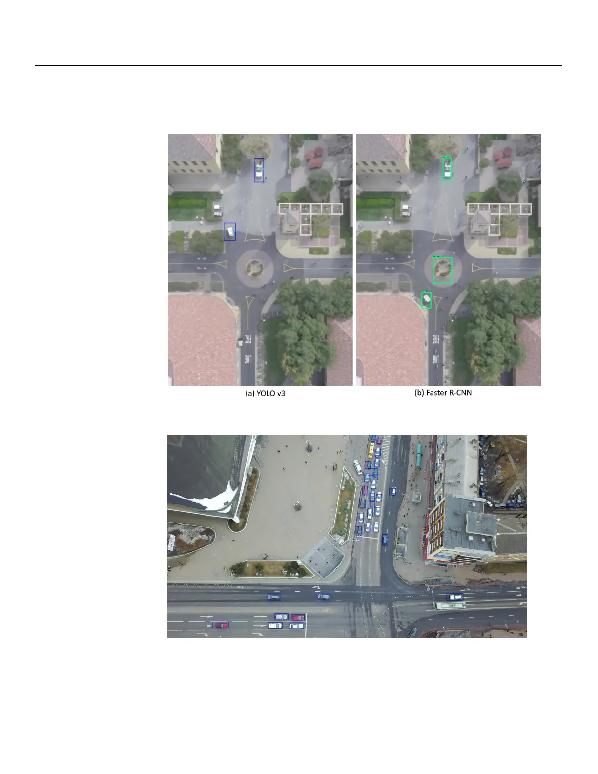
Article Aerial Images Processing for Car Detection using Convolutional Neural Networks: Comparison between Faster R-CNN and Y oloV3 Adel Ammar 1, * , Anis Koubaa 1,2, * , Mohanned Ahmed 1 , Abdulrahman Saad 1 and Bilel Benjdira 1,3        Citation: Ammar , A.; Koubaa, A.; Ahmed, M.; Saad, A.; Benjdira, B. Aerial Images Processing for Car Detection using Convolutional Neural Networks: Comparison between Faster R-CNN and Y oloV3. Journal Not Speciﬁed 2021 , 1 , 1. https://doi.org/ Academic Editor: Giovanni Dimauro Received: 21 February 2021 Accepted: 19 March 2021 Published: Publisher ’ s Note: MDPI stays neutral with regar d to jurisdictional claims in published maps and institutional afﬁl- iations. Copyright: © 2021 by the authors. Licensee MDPI, Basel, Switzerland. This article is an open access arti- cle distributed under the terms and conditions of the Creative Commons Attribution (CC BY) license (https:// creativecommons.or g/licenses/by/ 4.0/). 1 Department of Computer Science, College of Computer & Information Sciences, Prince Sultan University , 11586 Riyadh, Saudi Arabia; mohanned.ahmed@riotu-lab.org (M.A.); abdelrahman.saad@riotu-lab.or g (A.S.); bbenjdira@psu.edu.sa (B.B.) 2 CISTER Research Centr e, ISEP , Polytechnic Institute of Porto, 4200-465 Porto, Portugal 3 SEICT Lab, LR18ES44, Enicarthage, University of Carthage, T unis 1054, T unisia * Correspondence: aammar@psu.edu.sa (A.A.); akoubaa@psu.edu.sa (A.K.) Abstract: This paper addr esses the problem of car detection from aerial images using Convolutional Neural Networks (CNNs). This pr oblem presents additional challenges as compar ed to car (or any object) detection from gr ound images because the features of vehicles from aerial images ar e more dif ﬁcult to discern. T o investigate this issue, we assess the performance of three state-of-the-art CNN algorithms, namely Faster R-CNN, which is the most popular region-based algorithm, as well as YOLOv3 and YOLOv4, which ar e known to be the fastest detection algorithms. W e analyze two datasets with differ ent characteristics to check the impact of various factors, such as the UA V’s (unmanned aerial vehicle) altitude, camera resolution, and object size. A total of 52 training experiments were conducted to account for the ef fect of dif ferent hyperparameter values. The objective of this work is to conduct the most robust and exhaustive comparison between these thr ee cutting-edge algorithms on the speciﬁc domain of aerial images. By using a variety of metrics, we show that the dif ference between YOLOv4 and YOLOv3 on the two datasets is statistically insigniﬁcant in terms of A verage Pr ecision (AP) (contrary to what was obtained on the COCO dataset). However , both of them yield markedly better performance than Faster R-CNN in most conﬁgurations. The only exception is that both of them exhibit a lower recall when object sizes and scales in the testing dataset differ lar gely from those in the training dataset. Keywords: car detection; convolutional neural networks; deep learning; Faster R-CNN; unmanned aerial vehicles; YOLOv3; YOLOv4 1. Introduction Unmanned aerial vehicles (UA Vs) are nowadays a key enabling technology for a lar ge number of applications such as surveillance [ 1 ], tracking [ 2 ], disaster management [ 3 ], smart parking [ 4 ], and Intelligent T ransportation Systems [ 5 ], to name a few . Thanks to their versatility , UA Vs offer unique capabilities in collecting visual data using high-resolution cameras from differ ent locations, angles, and altitudes. These capabilities provide rich datasets of images that can be analyzed to extract useful information that serves the purpose of the underlying applications. Compar ed to ground images, UA V aerial imagery collection pr esents several advantages, including a lar ge ﬁeld of view , high spatial resolution, ﬂexibility , and high mobility . Although satellite imagery also provides a bird’s eye view of the earth, UA V -based aerial imagery presents several advantages as compared to satellite imagery . In fact, UA V imagery has a much lower cost and provides more updated views (many satellite maps are several months old and do not present recent changes). In addition, it can be used for Journal Not Speciﬁed 2021 , 1 , 1. https://doi.or g/10.3390/1010001 https://www .mdpi.com/journal/notspeciﬁed Journal Not Speciﬁed 2021 , 1 , 1 2 of 37 real-time image/video str eam analysis in a much more affor dable means. Aerial images have differ ent resolutions as compared to satellite images. For example, in our experiments, we reached a r esolution of 2 cm/pixel (and can have even lower) for aerial images using typical DJ (Shenzhen DJI Sciences and T echnologies Ltd. https://www .dji.com) drones, whereas satellite images have resolutions of about 15 cm/pixel as for the dataset described in [ 6 ] and can be even larger . W ith the current hype of artiﬁcial intelligence and deep learning, there has been an increasing trend since 2012 (the birth of AlexNet) to use Convolutional Neural Networks (CNNs) to extract information fr om images and video streams. While CNNs have been proven to be the best approach for classiﬁcation, detection, and semantic segmentation of images, aerial images have many peculiarities that differ fr om the classical types of images (ground- level images). For example, objects can be viewed from differ ent altitudes and viewpoints. Hence, a single class can have many patterns and repr esentations to be learned. This is deﬁned as high intra-class variance and indicates high variability in the appearances of objects belonging to the same class. Moreover , dif ferent classes can shar e comparable appearances, especially in high altitudes. This is deﬁned as low inter-class variance and makes the learning task more challenging. Recently , ther e have been several r esearch works that addr ess the pr oblem of car detection from aerial images [ 7 – 10 ]. In our previous work [ 1 ], we compared YOLOv3 and Faster R- CNN in detecting cars from aerial images. However , we only used one small dataset from low-altitude UA V images collected at the premises of Prince Sultan University . However , the altitude at which the image is taken plays an essential role in the accuracy of detection. In addition, we did not pr ofoundly analyze advanced and essential performance metrics such as Intersection over Union (IoU) and the Mean A verage Precision (mAP). In this paper , we address the gap, we consider multiple datasets with different conﬁgurations, and we also compare the newly released YOLOv4 object detector. Our objective is to present a more comprehensive analysis of the comparison between these thr ee state-of-the-art approaches (Faster R-CNN, YOLOv3, and YOLOv4). In [ 4 ], the authors mentioned the challenges faced with aerial images for car detection, namely the problem of having small objects and complex backgr ounds. They addressed the problem with the pr oposed Multi-task Cost-sensitive-Convolutional Neural Network based on Faster R-CNN. Other resear chers have addressed the problem applying deep learning techniques on aerial images, in such contexts as object detection and classiﬁcation [ 11 , 12 ], semantic segmentation [ 13 – 15 ], and generative adversarial networks (GANs) [ 16 ]. Jiao et al. [ 17 ] surveyed a large number of object detectors and r eported their results on the COCO dataset [ 18 ]. Our objective in this paper is different, since we focused on the depth- wise aspect of the comparison by selecting three r ecent algorithms that are r epresentative of the two main categories of object detectors, namely Faster R-CNN [ 19 ] (a two-stage detector) as well as YOLOv3 [ 20 ] and YOLOv4 [ 21 ] (one-stage detectors), examining a wide range of hyperparameters and assessing the effect of the size and characteristics of aerial view datasets. The contributions of this paper are as follows: First, we consider two different datasets of aerial images for the car detection problem with different characteristics to investigate the impact of dataset properties on the performance of the algorithms. In addition, we provide a thorough comparison between the thr ee most sophisticated categories of CNN approaches for object detection, Faster RCCN, which is a region-based approach pr oposed in 2017, YOLOv3, which is still the most popular version of the Y ou-Look-Only-Once approach proposed by Joseph Redmon in 2018, and the latest version YOLOv4, released by Bochkovskiy et al., in April 2020. The r emainder of this paper is or ganized as follows. Section 2 discusses the r elated works that deal with car detection and aerial image analysis using CNN, and some comparative Journal Not Speciﬁed 2021 , 1 , 1 3 of 37 studies applied to other object detections. Section 3 sets forth the theoretical backgr ound of the thr ee algorithms. Section 4 describes the datasets and the obtained results. Finally , Section 5 draws the main conclusions of this study . 2. Related W orks V arious techniques have been proposed in the literature to solve the problem of car detection in aerial images and similar related issues. The main challenge is the small size and the large number of objects in aerial views, which may lead to information loss when performing convolution operations, as well as a dif ﬁculty to discern features because of the angle of view . There are speciﬁc challenges for each type of aerial imagery (ﬁxed CCTV cameras, satellite, or UA V), due to their disparate level of resolution. W e pr esent here the most recent, r elevant works in object detection for each of these thr ee imagery types, and we then highlight the value added of the present work. 2.1. Fixed Surveillance Cameras Xi et al. [ 4 ] addressed the pr oblem of vehicle detection fr om overhead surveillance images. They proposed a multi-task appr oach based on the Faster R-CNN algorithm to which they added a cost-sensitive loss. The main idea was to subdivide the object detection task into simpler subtasks with enlarged objects, thus improving the detection of small objects that are frequent in aerial views. In addition, the cost-sensitive loss gives more importance to objects that are dif ﬁcult to detect or occluded because of a complex background and aims at improving the overall performance. Their method outperformed state-of-the-art techniques on their own speciﬁc, private dataset that was collected from surveillance cameras placed on top of buildings surr ounding a parking lot. However , their approach has not been tested on other datasets, nor on UA V images. In a similar application, Kim et al. [ 22 ] compar ed various implementations of CNN-based object detectors, namely YOLO (see Section 3.2.1 ), the Single Shot MultiBox Detector (SSD), the region-based convolutional neural network (R-CNN), the region-based Fully Convolutional Neural Network (R-FCN), and SqueezeDet [ 23 ] (based on a Fully Convolutional Neural Network). They applied these algorithms on the problem of person detection, and trained and tested them on their own in-house dataset composed of images that were captured by surveillance cameras in retail stores. They found that YOLOv3 (with a 416 input size) and SSD (with a VGG-500 feature extractor) [ 24 ] provide the best tradeof f between accuracy and response latency . In [ 25 ], Hardjono et al. investigated the problem of automatic vehicle counting in CCTV images collected from four datasets with various resolutions. On the one hand, they tested two classical image processing techniques: Background Subtraction (which calculates a for eground mask by subtracting a background model from the image) and the V iola Jones Algorithm [ 26 ] (combining Haar-like Features, Integral Images, AdaBoost Algorithm [ 27 ], and Cascading Classiﬁer), with Median or Gaussian Filters. On the other hand, they also applied deep learning neural networks, namely YOLOv2 [ 28 ] and FCRN Fully Convolutional Regr ession Network) [ 29 ]. Their results show that deep learning techniques yield markedly better detection results (in terms of F1 scor e) when applied on higher resolution datasets. 2.2. Satellite Imagery Chen et al. [ 30 ] applied a technique based on a Hybrid Deep Convolutional Neural Network(HDNN) and a sliding window search to solve the vehicle detection problem fr om Google Earth images. The maps of particular layers of the CNN (last convolutional layer and max-pooling layer) are split into blocks of variable ﬁeld sizes, so as to be able to extract features of various scales. In addition, they modiﬁed the sliding windows to contain the main Journal Not Speciﬁed 2021 , 1 , 1 4 of 37 part of the vehicle to be detected. Thus, they obtained an improved detection rate compar ed to the traditional deep architectur es at that time, but with the expense of a high execution time (7 s per image, using a GPU). For the aim of car counting, Mundhenk et al. [ 6 ] built their own Cars Over head with Con- text (COWC) dataset containing 32,716 unique cars and 58,247 negative targets, standardized to a resolution of 15 cm per pixel, and annotated using single pixel points. The authors used a Convolutional Neural Network that they called ResCeption, based on Inception synthesized with Residual Learning. The main modiﬁcation to the Inception architecture is the substitu- tion of 1 × 1 convolutions by residual pr ojection shortcuts. The model was able to count the number of cars in test patches with a root mean square error of 0.66 at 1.3 FPS (frames per second). 2.3. UA V Imagery Relatively fewer works have addressed the problem of car detection fr om UA V images. Ammour et al. [ 31 ] used a pre-trained CNN coupled with a linear support vector machine (SVM) classiﬁer to detect and count cars in high-resolution UA V images of urban areas. First, the input image is segmented into candidate regions using the mean-shift algorithm. The VGG16 [ 32 ] CNN model is then applied to windows that are extracted around each candidate region to generate descriptive features, that are subsequently classiﬁed using a linear SVM binary model. Finally , they applied a ﬁne-tuning morphological dilation for smoothing the detected regions. This multi-stage technique achieved state-of-the-art performance on a reduced testing dataset (5 images containing 127 car instances), but it still falls short of real- time processing, mainly due to the high computational cost of the mean-shift segmentation stage. Liu and Mattyus [ 8 ] focused on ﬁne-grained car detection. They used a soft-cascade structur e of integral channel features [ 33 ] to classify car orientations and types (car or truck) in a dataset of aerial images of the city of Munich consisting of 20 images taken at an altitude of 1000 m with a resolution of 5616 × 3744 and a GSD (Ground Sampling Distance) of 13 cm. They obtained an accuracy of 98% at a processing time of 4.4 s per image, which is faster than traditional techniques such as V iola Jones, but still far from real time. Such classiﬁcation can be used for the urban planning, trafﬁc management, census estimation, and sociological analysis of cities and countries. 2.4. Our Contribution T able 1 summarizes the datasets, algorithms, and results of the most similar related works on car detection, compared to the present paper . The closest work to the present study is that of Benjedira et al. [ 1 ] who presented a performance evaluation of Faster R-CNN and YOLOv3 algorithms, on a reduced UA V imagery dataset of cars. The present paper is an improvement over this work from several aspects: (1) W e use two datasets with different characteristics for training and testing, whereas most previous works described above tested their technique on a single proprietary dataset. W e show that annotation err ors in the dataset have an important effect on the detection performance. (2) W e added a thir d algorithm (YOLOv4) to the comparative analysis. (3) W e tested various hyperparameter values (three dif ferent input sizes for YOLOv3 and YOLOv4 each, two differ ent feature extractors for Faster R-CNN, and various values of score and IoU thr esholds). (4) W e conducted a more detailed comparison of the results, by showing the AP at differ ent values of IoU thresholds, comparing the tradeof f between AP and inference speed, and calculating several new metrics that have been suggested for the COCO dataset [ 18 ]. Journal Not Speciﬁed 2021 , 1 , 1 5 of 37 T able 1. Comparison of our paper with the related works. Ref. Dataset Used Algorithms Main Results [ 6 ] Mundhenk et al., 2016 Cars Overhead with Context (COWC): 32,716 unique cars. 58,247 negative targets. 308,988 training patches and 79,447 testing patches. Annotated using single pixel points. Resolution: 1024 × 1024 and 2048 × 2048. ResCeption (Inception with Residual Learning) Up to 99.14% correctly classiﬁed patches (containing cars or not). F1 score of 94.34% for detection. Car counting: RMSE of 0.676. [ 4 ] Xi et al., 2019 Parking lot dataset from aerial view . T raining: 2000 images. T esting: 1000 images. Number of instances: NA. Resolution: 5456 × 3632. Multi-T ask Cost-sensitive Convolutional Neural Network (MTCS-CNN). mAP of 85.3% for car detection. [ 30 ] Chen et al., 2014 63 satellite images collected from Google Earth. T raining: 31 images (3901 vehicles). T esting: 32 images (2870 vehicles). Resolution: 1368 × 972. Hybrid Deep Convolutional Neural Network (HDNN). Precision up to 98% at a recall rate of 80%. [ 31 ] Ammour et al., 2017 8 images acquired by UA V . T raining: 3 images (136 positive instances, and 1864 negative instances). T esting: 5 images (127 positive instances). Resolution: V ariable fr om 2424 × 3896 to 3456 × 5184. Spatial resolution of 2 cm. Pre-trained CNN coupled with a linear support vector machine (SVM). Precision from 67% up to 100%, and recall from 74% up to 84%, on the ﬁve testing images. Inference time: between 11 and 30 min/image. [ 25 ] Hardjono et al., 2018 4 CCTV datasets: - Dataset 1: 3 s videos at 1 FPS. Resolution: 480 × 360 - Dataset 2: 60 min:32 sec video at 9 FPS. Resolution: 1920 × 1080 - Dataset 3: 30 min:27 sec video at 30 FPS. Resolution: 1280 × 720 - Dataset 4: 32 sec video at 30 FPS. Resolution: 1280 × 720 T raining: 1932 positive instances and 10,000 negative instances. - Background Subtraction (BS) - V iola Jones (VJ) - YOLOv2 - BS: F1 score from 32% to 55%. Inference time from 23 to 40 ms. - VJ: F1 score from 61% to 75%. Inference time from 39 to 640 ms. - YOLOv2: F1 score from 92% to 100% on Datasets 2 to 4. Inference time not reported. [ 1 ] Benjdira et al., 2019 PSU+[27] UA V dataset: T raining: 218 images (3365 car instances). T esting: 52 images (737 car instances). Resolution: V ariable fr om 684 × 547 to 4000 × 2250. - YOLOv3 (input size: 608 × 608). - Faster R-CNN (Feature extractor: Inception ResNet v2). - YOLOv3: F1 score of 99.9%. Inference time: 57 ms. - Faster R-CNN: F1 score of 88%. Inference time: 1.39 s. (Using an Nvidia GTX 1080 GPU). Our paper - Stanford UA V dataset: T raining: 6872 images (74,826 car instances). T esting: 1634 images (8131 car instances). Resolution: V ariable from 1184 × 1759 to 1434 × 1982. PSU+[27] UA V dataset: T raining: 218 images (3365 car instances). T esting: 52 images (737 car instances). Resolution: V ariable from 684 × 547 to 4000 × 2250. - YOLOv3 and YOLOv4 (input sizes: 320 × 320, 416 × 416, and 608 × 608). - Faster R-CNN (Feature extractors: Inception v2, and Resnet50). - YOLOv4: F1 score: up to 34.4% on the Stanford dataset up to 94.6% on the PSU dataset. Inference time: from 45 to 80 ms. - YOLOv3: F1 score: up to 32.6% on the Stanford dataset up to 96.0% on the PSU dataset. Inference time: from 43 to 85 ms. - Faster R-CNN: F1 score: up to 31.4% on the Stanford dataset up to 84.5% on the PSU dataset. Inference time: from 52 to 160 ms. (Using an Nvidia GTX 1080 GPU). 3. Theoretical Overview of Faster R-CNN and YOLO Architectures Object detection is an old fundamental problem in image pr ocessing, for which various approaches have been applied. However , since 2012, deep learning techniques have markedly outperformed classical ones. The object detection algorithms based on deep learning are classiﬁed into two large branches: two-stage detectors and one-stage detectors. From each of these two branches, we selected, in this study , the best performing algorithms. W e selected in the ﬁrst branch, Faster R-CNN [ 19 ], which is the most r epresentative model fr om the two-stage family , according to [ 34 ]. In the second branch, we selected the YOLO algorithm and picked out its most recent versions: YOLO v3 [ 20 ] and YOLO v4 [ 21 ]. The selected algorithms have been proven successful in terms of of accuracy and speed in a wide variety of applications. . 3.1. T wo-Stage Detector: Faster R-CNN R-CNN, as coined by [ 35 ], is a Convolutional Neural Network (CNN) combined with a region-pr oposal algorithm that hypothesizes object locations. It initially extracts a ﬁxed number of regions (2000), by means of a selective search. It then merges similar regions to- gether , using a greedy algorithm, to obtain the candidate regions on which the object detection will be applied. Afterwards, the same authors proposed an enhanced algorithm called Fast Journal Not Speciﬁed 2021 , 1 , 1 6 of 37 R-CNN [ 36 ] by using a shared convolutional feature map that the CNN generates directly from the input image, and fr om which the regions of interest (RoI) ar e extracted. Finally , Ren et al. [ 19 ] proposed a Faster R-CNN algorithm that intr oduced a Region Proposal Network (RPN), which is a dedicated fully convolutional neural network that is trained end-to-end (Figure 1 ) to predict both object bounding boxes and objectness scor es in an almost compu- tationally cost-free manner (around 10 ms per image). This important algorithmic change thus replaced the selective search algorithm, which was very computationally expensive and repr esented a bottleneck for previous object detection deep learning systems. As a further optimization, the RPN ultimately shares the convolutional features with the Fast R-CNN detector , after ﬁrst being independently trained. For training the RPN, Faster R-CNN kept the multi-task loss function already used in Fast R-CNN [ 36 ]. Faster R-CNN uses three scales and three aspect ratios for every sliding position, and is translation-invariant. In addition, it conserves the aspect ratio of the original image while resizing it, so that one of its dimensions is 1024 or 600. Figure 1. Region Proposal Network (RPN) architectur e. 3.2. One-Stage Detectors W e have considered two networks of the one-stage category: YOLOv3 and YOLOv4. W e ﬁrst describe the architectur e of YOLOv3 and then brieﬂy enumerate the enhancements made in YOLOv4. 3.2.1. YOLOv3 Contrary to R-CNN variants, YOLO [ 37 ], which is an acronym for Y ou Only Look Once, does not extract region pr oposals, but processes the complete input image only once using a Fully Convolutional Neural Network that predicts the bounding boxes and their corre- sponding class probabilities, based on the global context of the image. The ﬁrst version was published in 2016. Later on in 2017, a second version, YOLOv2 [ 28 ], was proposed, which intro- Journal Not Speciﬁed 2021 , 1 , 1 7 of 37 duced batch normalization, a retuning phase for the classiﬁer network, and dimension clusters as anchor boxes for predicting bounding boxes. Finally , in 2018, YOLOv3 [ 20 ] improved the detection further by adopting several new features: • Replacing the mean squared error by cross-entr opy for the loss function. The cross- entropy loss function is calculated as follows: − M ∑ c = 1 δ x ∈ c l o g ( p ( x ∈ c )) (1) where M is the number of classes, c is the class index, x is an observation, δ x ∈ c is an indicator function that equals 1 when c is the correct class for the observation x , and l o g ( p ( x ∈ c )) is the natural logarithm of the predicted probability that observation x belongs to class c . • Using logistic r egression (instead of the softmax function) for predicting an objectness score for every bounding box. • Using a signiﬁcantly larger feature extractor network with 53 convolutional layers (Darknet-53 replacing Darknet-19). It consists mainly of 3 × 3 and 1 × 1 ﬁlters, with some skip connections (Figure 2 ) inspir ed from ResNet [ 38 ]. Contrary to Faster R-CNN’s approach, each gr ound-truth object in YOLOv3 is assigned only one bounding box prior . These successive variants of YOLO wer e developed with the objective of obtaining a maximum mAP while keeping the fastest execution that makes it suitable for real-time applications. Special emphasis has been put on execution time, so that YOLOv3 is equivalent to state-of-the-art detection algorithms such as SSD [ 24 ] in terms of accuracy but with the advantage of being three times faster [ 20 ]. Figure 3 depicts the main stages of the YOLOv3 algorithm when applied to the car detection problem. V ariable input sizes are allowed in YOLO. W e have tested the thr ee input sizes that are usually used (as in the original YOLOv3 paper [ 20 ]): 320 × 320, 416 × 416, and 608 × 608. Figure 2. YOLOv3 architecture. Journal Not Speciﬁed 2021 , 1 , 1 8 of 37 Figure 3. Successive stages of the YOLOv3 model applied on car detection. 3.2.2. YOLOv4 YOLOv4 [ 21 ] was introduced after two years of cumulative improvements over YOLOv3 [ 20 ], leveraging the recent advances in deep learning. It achieves an accuracy of 43.5% AP on the MS COCO dataset compared to 33.0% AP for YOLOv3. This high accuracy is made while keeping a very efﬁcient infer ence time (65 FPS on T esla V100). YOLOv4 aims to make object detection run efﬁciently and smoothly on the low-cost hardwar e provided on most edge devices. Concerning the technical impr ovements made in YOLOv4, they are classiﬁed into two categories. The ﬁrst categ ory is named the Bag of Freebies (BoF) and designates improvements that can be made during training without affecting the inference time. This includes Cut- Mix [ 39 ] and Mosaic data augmentation techniques, DropBlock regularization [ 40 ], class label smoothing, Complete IoU (CIoU) loss [ 41 ], Cross mini-Batch Normalization (CmBN) [ 42 ], Self Adversarial T raining (SA T), multiple anchors for a single ground tr uth, cosine annealing scheduler [ 43 ], and optimal hyper-parameters obtained thr ough genetic algorithms. On the other hand, the second category is named Bag of Specials (BoS) and r epresents improvements that slightly affect the inference time while making a considerable increase in accuracy . This includes the mish activation function [ 44 ], Cross Stage Partial connections (CSP)) [ 45 ], Multi-input W eighted Residual Connection (MiWRC) [ 46 ], the Spatial Pyramid Pooling (SPP) block [ 47 ], the Spatial Attention Module (SAM) block [ 48 ], the Path Aggregation Network (P AN) block [ 49 ], and the Distance IoU Loss (DIoU) [ 41 ] used as a factor in the Non-Maximum-Suppression (NMS) step. T o summarize, T able 2 compar es the features and parameters of Faster R-CNN, YOLOv3, and YOLOv4. While successive optimizations and mutual inspirations made the methodology of the two architectures relatively close, the main difference remains that Faster R-CNN has two separate phases of region proposals and classiﬁcation (although now with shared features), whereas YOLO has always combined the classiﬁcation and bounding-box regression processes. Journal Not Speciﬁed 2021 , 1 , 1 9 of 37 T able 2. Theoretical comparison of YOLOv3, YOLOv4, and Faster R-CNN. YOLOv3 YOLOv4 Faster R-CNN Phases Concurrent bounding box regr ession, and classiﬁcation Concurrent bounding box regr ession, and classiﬁcation RPN + Fast R-CNN object detector Neural network type Fully convolutional. Fully convolutional. Fully convolutional (RPN and 4 detection network). Backbone feature extractor Darknet-53 (53 convolutional layers). CSPDarknet53 (53 convolutional layers). VGG-16 or Zeiler & Fergus(ZF). Other feature extractors can also be incorporated. Location detection Anchor-based (dimension clusters). Anchor-based Anchor-based Number of anchors boxes Only one bounding-box prior for each ground-truth object. Using multiple anchors for a single ground truth 3 scales and 3 aspect ratios, yielding k = 9 anchors at each sliding position. Default Anchors sizes (10,13), (16,30), (33,23), (30,61), (62,45), (59,119), (116,90), (156,198), (373,326) (12,16), (19,36), (40,28), (36,75), (76,55), (72,146), (142,110), (192,243), (459,401) Scales: (128,128), (256,256), (512,512). Aspect ratios: 1:1, 1:2, 2:1. IoU thresholds One (at 0.5). One (at 0.213) T wo (at 0.3 and 0.7). Loss function Binary cross-entr opy loss Complete IoU loss: CIoU Multi-task loss: - Log loss for classiﬁcation. - Smooth L1 for regr ession. Input size Differ ent possible input sizes (n × n with n multiple of 32). Differ ent possible input sizes (n × n with n multiple of 32). - Conserves the aspect ratio of the original image. - Either the smallest dimension is 600, or the largest dimension is 1024. Momentum Default value: 0.9. Default value: 0.949 Default value: 0.9. W eight decay Default value: 0.0005. Default value: 0.0005 Default value: 0.0005. Batch size Default value: 64. Default value: 64. Default value: 1. 4. Experimental Comparison between Faster R-CNN , YOLOv3, and YOLOv4 In this section, we will ﬁrst describe the two datasets used for training and testing, and the hyperparameters chosen for each algorithm, and then present and discuss the results obtained. 4.1. Datasets In order to obtain a robust comparison, we tested the Faster R-CNN, YOLOv3, and YOLOv4 algorithms on two datasets of aerial images showing completely different character - istics. • The Stanford dataset [ 50 ] consists of a large-scale collection of aerial images and videos of a university campus containing various agents (cars, buses, bicycles, golf carts, skate- Journal Not Speciﬁed 2021 , 1 , 1 10 of 37 boarders, and pedestrians). It was obtained using a 3DR SOLO quadcopter (equipped with a 4k camera) that ﬂew over various cr owded campus scenes, at an altitude of around 80 m. It is originally composed of eight scenes, but since we are exclusively interested in car detection, we chose only thr ee scenes that contains the lar gest percentage of cars: Nexus (in which 29.51% of objects are cars), Gates (1.08%), and DeathCir cle (4.71%). All other scenes contain less than 1% of cars. W e used the two ﬁrst scenes for training and the third one for testing. In addition, we removed images that contain no cars. T able 3 shows the number of images and instances in the training and testing datasets. The images in the selected scene have variable sizes, as shown in T able 4 , and contain cars of various sizes, as depicted in Figure 4 . The average car size (calculated based on the ground-truth bounding boxes) is shown in T able 5 . The discr epancy observed between the training and testing datasets in terms of car sizes is explained by the fact that we used different scenes for the training and testing datasets, as explained above. This discrepancy will constitute an additional challenge for the considered object detection algorithms. Furthermore, we noticed that the ground-truth bounding boxes in some images contain some mistakes (bounding boxes containing no objects) and imprecisions (many bounding boxes are much larger than the objects inside them), as can be seen in Figur e 5 , but we used them as they are in or der to assess the impact of annotation err ors on detection performance. In fact, the Stanford Dr one Dataset was not primarily designed for object detection, but for trajectory forecasting and tracking. T able 3. Number of images and car instances in Stanford and PSU (Prince Sultan University) datasets. Stanford Dataset PSU Dataset T raining Set T esting Set T otal T raining Set T esting Set T otal Number of images 6872 1634 8506 218 52 270 Percentage 80.8% 19.2% 100% 80.7% 19.3% 100% Number of car instances 74,826 8131 82,957 3364 738 4102 T able 4. Image size in the Stanford dataset. Size Number of Images 1409 × 1916 1634 1331 × 1962 1558 1330 × 1947 1557 1411 × 1980 1494 1311 × 1980 1490 1334 × 1982 295 1434 × 1982 142 1284 × 1759 138 1425 × 1973 128 1184 × 1759 70 T able 5. A verage car width and length (in pixels) in the PSU and Stanford datasets, calculated based on the ground-truth bounding boxes. Dataset A verage Car Width A verage Car Length PSU training 48 36 PSU testing 55 46 Stanford training 72 152 Stanford testing 60 90 Journal Not Speciﬁed 2021 , 1 , 1 11 of 37 Journal Not Speciﬁed 2021 , 1 , 1 12 of 37 Figure 4. Histogram of car sizes in PSU (a,c) and Stanfor d (b,d) training (a,b) and testing (c,d) datasets, expressed as the number pixels inside the ground truth bounding boxes (width × height). Journal Not Speciﬁed 2021 , 1 , 1 13 of 37 Figure 5. A sample image of the Stanford dataset, with ground-truth bounding boxes showing some annotation errors and impr ecisions. • The PSU datasetwas collected from two sour ces: an open dataset of aerial images avail- able on Github [ 51 ] and our own images acquired after ﬂying a 3DR SOLO drone equipped with a GoPro Hero 4 camera, in an outdoor environment at a PSU parking lot. The drone r ecorded videos from which frames were extracted and manually labeled. Since we are only inter ested in a single class, images with no cars were r emoved from the dataset. The training/testing split was made randomly . T able 3 shows the number of images and instances in the training and testing datasets. The dataset thus obtained contains images of different sizes, as shown in T able 6 , and contains cars of various sizes, as depicted in Figure 4 . The average car size (calculated based on the ground-truth bounding boxes) in the training and testing datasets is shown in T able 5 . W e have made this dataset available on [ 52 ]. T able 6. Image size in the PSU dataset. Size Number of Images 1920 × 1080 172 1764 × 430 26 684 × 547 21 1284 × 377 20 1280 × 720 19 4000 × 2250 12 4.2. Hyperparameters The main hyperparameter for YOLOv3 and YOLOv4 networks is the input size, for which we tested three values (320 × 320, 416 × 416, and 608 × 608), as explained in Section 3.2.1 . Journal Not Speciﬁed 2021 , 1 , 1 14 of 37 On the other hand, the main hyperparameter for Faster R-CNN is the feature extractor . W e tested two different feature extractors: Inception-v2 [ 53 ] (also called BN-inception in the literature [ 54 ]) and Resnet50 [ 38 ]. As explained in Section 3.1 , the default setting of Faster R-CNN conserves the aspect ratio of the original image while resizing it, so that one of its dimensions is 1024 or 600. However , to be able to fairly compare its precision and speed with YOLO algorithms, which use ﬁxed input sizes, we also tested Faster R-CNN with a ﬁxed input size of 608 × 608, for each of the two featur e extractors. These settings make a total of 10 classiﬁers that we trained and tested on the two datasets described above, which amounts to 20 experiments, summarized in T able 7 . In these experiments, we kept the default values for the momentum (0.9), weight decay (0.0005), learning rate (initial rate of 10 − 3 for YOLOv3 and YOLOv4, 2 × 10 − 4 for Faster R-CNN with Inception-v2, and 3 × 10 − 4 with Resnet50), batch size (64 for YOLOv3 and YOLOv4, and 1 for Faster R-CNN), and anchor sizes (see T able 2 ). Furthermore, we conducted additional experiments with differ ent values of learning rates (10 − 5 , 10 − 4 , 10 − 3 , and 10 − 2 ) for each of the main algorithms (Faster R-CNN with Inception-v2, Faster R-CNN with Resnet 50, YOLOv3, and YOLOv4 with the input size 416 × 416), on each of the two datasets. W e trained each network for the number of iterations necessary to its convergence. W e notice, for example, in T able 7 that YOLOv3 necessitated a higher number of iterations when using the largest input size (608 × 608) on the Stanford dataset, while it reached conver gence after much fewer iterations when using the medium input size (416 × 416) on the same dataset. Meanwhile, YOLOv4 converges much faster in all conﬁgurations due to the use of the cosine annealing scheduler described in Section 3.2.2 . Nevertheless, the number of steps needed to r each convergence is non-deterministic and depends on the initialization of the weights. Journal Not Speciﬁed 2021 , 1 , 1 15 of 37 T able 7. Details of the main experiments. The default conﬁguration of Faster R-CNN allows for a variable input size that conserves the aspect ration of the image. In this case, the input size shown is an average. # Algorithm Feature Extractor Dataset A verage Input Size Number of Iterations 1 Faster R-CNN Inception v2 Stanford 816 × 600 (variable) 600,000 2 Faster R-CNN Inception v2 PSU 992 × 550 (variable) 600,000 3 Faster R-CNN Resnet50 Stanford 816 × 600 (variable) 600,000 4 Faster R-CNN Resnet50 PSU 992 × 550 (variable) 600,000 5 Faster R-CNN Inception v2 Stanford 608 × 608 (ﬁxed) 600,000 6 Faster R-CNN Inception v2 PSU 608 × 608 (ﬁxed) 600,000 7 Faster R-CNN Resnet50 Stanford 608 × 608 (ﬁxed) 600,000 8 Faster R-CNN Resnet50 PSU 608 × 608 (ﬁxed) 600,000 9 YOLO v3 Darknet-53 Stanford 320 × 320 (ﬁxed) 896,000 10 YOLO v3 Darknet-53 Stanford 416 × 416 (ﬁxed) 320,000 11 YOLO v3 Darknet-53 Stanford 608 × 608 (ﬁxed) 1,088,000 12 YOLO v3 Darknet-53 PSU 320 × 320 (ﬁxed) 640,000 13 YOLO v3 Darknet-53 PSU 416 × 416 (ﬁxed) 640,000 14 YOLO v3 Darknet-53 PSU 608 × 608 (ﬁxed) 640,000 15 YOLO v4 CSPDarknet-53 Stanford 320 × 320 (ﬁxed) 192,000 16 YOLO v4 CSPDarknet-53 Stanford 416 × 416 (ﬁxed) 192,000 17 YOLO v4 CSPDarknet-53 Stanford 608 × 608 (ﬁxed) 192,000 18 YOLO v4 CSPDarknet-53 PSU 320 × 320 (ﬁxed) 192,000 19 YOLO v4 CSPDarknet-53 PSU 416 × 416 (ﬁxed) 192,000 20 YOLO v4 CSPDarknet-53 PSU 608 × 608 (ﬁxed) 192,000 4.3. Results and Discussion For the experimental setup, we used a workstation powered by an Intel core i7-8700K (3.7 GHz) pr ocessor , with 32 GB RAM, and an NVIDIA GeFor ce 1080 (8 GB) GPU, running on Linux. W e will ﬁrst explain the metrics used for the evaluation, then discuss the results of each metric for each algorithm on each testing dataset described above. W e also tested differ ent learning rates and anchor scales in order to assess the algorithms’ sensitivity to these hyperparameters. A total of 52 trainings have been conducted (20 experiments with default hyperparameters, 28 experiments with differ ent learning rates, and 4 experiments with differ ent anchor scales). 4.3.1. Metrics The following metrics have been used to assess the results: • IoU: Intersection over Union measuring the overlap between the predicted and the ground-tr uth bounding boxes. Journal Not Speciﬁed 2021 , 1 , 1 16 of 37 • mAP: mean average precision, or simply AP , since we are dealing with only one class. It corresponds to the area under the precision vs. recall curve. AP was measured for differ ent values of IoU (0.5, 0.6, 0.7, 0.8, and 0.9). • FPS: number of frames per second, measuring the inference pr ocessing speed. • Inference time (in millisecond per image): also measuring the processing speed. I n f er e nc e t i me ( m s ) = 1000 F P S • AR max=1 , AR max=10 , and AR max=100 : average recall, when considering a maximum num- ber of detections per image, averaged over all values of IoU speciﬁed above. W e allow only the 1, 10, or 100 top-scoring detections for each image. This metric penalizes missing detections (false negatives) and duplicates (several bounding boxes for a single object). 4.3.2. A verage Precision When analyzing the r esults, it appears that all three tested algorithms gave a much better AP on the PSU dataset than on the Stanford dataset (Figure 6 ). This is mainly due to the fact that, contrary to the PSU dataset, the characteristics of the Stanford dataset differ lar gely between the training and testing images, as detailed in IV .A. This is the well known problem of domain adaptation in machine learning [ 16 ]. The Stanford dataset contains 20 times mor e car instances than the PSU dataset (T ables 3 ), whereas the performance of Faster R-CNN, YOLOv3, and YOLOv4 algorithms was r espectively four , seven, and ﬁve times better on the PSU dataset, in terms of AP . This highlights the fact that the clarity of the features, the quality of annotation, and the representativity of the learning dataset are mor e important than the actual size of the dataset. Faster RCNN YOLOv3 YOLOv4 0.0 0.2 0.4 0.6 0.8 Average AP 0.71 0.193 0.919 0.135 0.943 0.175 Average AP PSU Dataset Stanford Dataset Figure 6. Comparison of the AP (A verage Precision) between YOLOv3, YOLOv4, and Faster R-CNN. However , Figure 7 shows that the number of false negatives (non-detected cars) is much higher than the number of false positives on the Stanford dataset (3 times higher for Faster R-CNN, 73 times higher for YOLOv3, and 66 times higher for YOLOv4), and much higher than the number of true positives, which indicates that most cars go undetected in the Stanford dataset, most likely due to the differ ent size and aspect ratio of the cars in the testing images, compared to the training images. This is also visible on Figure 8 , which illustrates the trade-off between precision and recall for different score thresholds. While the precision is close to 1 for YOLOv3 and YOLOv4, but signiﬁcantly lower for Faster R-CNN, all the algorithms Journal Not Speciﬁed 2021 , 1 , 1 17 of 37 have a recall inferior to 0.25 on the Stanford dataset. On the contrary , Figure 9 shows high values of recall for YOLOv3 and YOLOv4, and a slightly lower precision compar ed to Faster R-CNN, on the PSU dataset. Even though all three algorithms performed poorly on the Stanford dataset as compared to the PSU dataset, with less than 20% of AP , there is still a statistically signiﬁcant differ ence between Faster R-CNN and YOLOv3 on this dataset. In fact, a T -test between the two sets of AP values of the two algorithms (for differ ent IoU and score thresholds) yielded a p-value of 0.0020, which means that the null hypothesis (equality of the means of the two sets of AP values) can be rejected with a conﬁdence of 99.8%. Meanwhile, the p-value between YOLOv3 and YOLOv4 AP values is 0.72, which means that the dif ference in performance between these two algorithms is not statistically signiﬁcant, as opposed to the large improvement that Bochkovskiy et al. [ 21 ] obtained on the COCO dataset. This result may indicate that YOLOv4 has been speciﬁcally tuned for the COCO dataset and does not perform as well on other datasets in terms of AP . FP TP FN 0 1000 2000 3000 4000 5000 6000 7000 Average value 14 528 209 PSU Dataset FP TP FN 1875 1715 6415 Stanford Dataset FP TP FN 44 688 49 PSU Dataset FP TP FN 96 1129 7001 Stanford Dataset FP TP FN 71 708 29 PSU Dataset FP TP FN 101 1463 6667 Stanford Dataset Faster RCNN YOLO v3 YOLO v4 Figure 7. A verage number of false positives (FP), false negatives (FN), and true positives (TP) for YOLOv3, YOLOv4, and Faster R-CNN on the two datasets. Journal Not Speciﬁed 2021 , 1 , 1 18 of 37 Figure 8. Precision vs. Recall for different values of scor e threshold (0.3, 0.5, 0.7, and 0.9), and IoU = 0.6 (Intersection over Union), on the Stanford dataset. Figure 9. Precision vs. Recall for different values of scor e threshold (0.3, 0.5, 0.7, and 0.9), and IoU = 0.6 (Intersection over Union), on the PSU dataset. Figure 10 shows examples of YOLOv3 and Faster R-CNN misclassiﬁcations on a sample image of the Stanford dataset. The false positives shown may be explained by the presence of errors of annotations in the learning dataset, as mentioned in Section 4.1 . Figures 11 and 12 Journal Not Speciﬁed 2021 , 1 , 1 19 of 37 show examples of YOLOv3 and Faster R-CNN misclassiﬁcations (all of them false negatives) on a sample image of the PSU dataset, respectively . YOLOv4 yields almost equivalent misclassiﬁcations, compared to YOLOv3. Figure 10. E x a m p l e o f ( a ) Y O L O v 3 a n d ( b ) Fa st er R - C N N ’ s o u t p u t o n a s a m p l e i m a g e o f th e S t a n f o r d d a t a s e t . Figure 11. Example of YOLOv3’s output on an image of the PSU dataset, showing a few false negatives (non-detected cars). Journal Not Speciﬁed 2021 , 1 , 1 20 of 37 Figure 12. Example of Faster R-CNN misclassiﬁcations on an image of the PSU dataset, showing several false negatives (non-detected cars). 4.3.3. A verage Recall T able 8 shows the average r ecall for a given maximum number of detections (as described in the introduction of Section 4.3 ), on the Stanfor d dataset. YOLOv4 (with medium and high input size) shows the best results in this metric, while the small input size (320 × 320) shows a marked inferior performance for both YOLOv3 and YOLOv4. The fact that the columns AR max=10 and AR max=100 in this table are identical can be explained by the fact that very few images in the Stanfor d testing dataset contain more than 10 car instances. Nevertheless, we have kept this duplicated column to compare it to T able 9 , which shows the same metrics on the PSU dataset. YOLOv4 (with any input size) is signiﬁcantly better in terms of the three metrics on this dataset, which indicates that YOLOv4 is better at detecting a high number of objects in a single image. T able 8. A verage recall for a given maximum number of detections, averaged over all values of IoU (0.5, 0.6, 0.7, 0.8, and 0.9) (Intersection over Union), on the Stanfor d dataset. The best results ar e marked in bold. Network AR max=1 AR max=10 AR max=100 Faster R-CNN (Inception-v2) 15.1% 17.1% 17.1% Faster R-CNN (Resnet50) 16.4% 18.6% 18.6% YOLOv3 (320 × 320) 9.0% 9.1% 9.1% YOLOv3 (416 × 416) 17.1% 17.3% 17.3% YOLOv3 (608 × 608) 17.2% 17.3% 17.3% YOLOv4 (320 × 320) 14.7% 14.7% 14.7% YOLOv4 (416 × 416) 19.3% 19.4% 19.4% YOLOv4 (608 × 608) 19.1% 24.0% 24.0% Journal Not Speciﬁed 2021 , 1 , 1 21 of 37 T able 9. A verage recall for a given maximum number of detections, averaged over all values of IoU (0.5, 0.6, 0.7, 0.8, and 0.9), on the PSU dataset. The best results are marked in bold. Network AR max=1 AR max=10 AR max=100 Faster R-CNN (Inception-v2) 6.2% 41.5% 70.8% Faster R-CNN (Resnet50) 6.4% 41.5% 67.2% YOLOv3 (320 × 320) 6.0% 42.2% 81.0% YOLOv3 (416 × 416) 6.4% 44.1% 90.4% YOLOv3 (608 × 608) 6.4% 44.5% 91.9% YOLOv4 (320 × 320) 6.8% 47.1% 95.5% YOLOv4 (416 × 416) 6.8% 46.8% 96.6% YOLOv4 (608 × 608) 6.7% 46.5% 95.6% 4.3.4. Inference Speed Figure 13 depicts the inference speed measur ed in frames per second (FPS), for each of the tested algorithms on both datasets. It shows that all conﬁgurations of YOLOv3 and YOLOv4 are signiﬁcantly faster than Faster R-CNN. Moreover , the input size has a direct impact on the inference time, as expected, since a larger input size generates a greater number of network parameters, and hence a larger number of operations. In fact, the inference processing speed of both YOLOv3 and YOLOv4 largely depends on the input size (from 12 FPS for 608 × 608 up to 23 FPS for 320 × 320), with little variation between the two datasets. As for Faster R-CNN, the Inception v2 feature extractor is 2.3 and 1.5 times faster on the Stanford and PSU datasets, respectively . The differ ence in speed when applying these algorithms on the two datasets is explained by the difference of image input size. In fact, we calculated that the average number of pixels in the input test images (after resizing) is 544,000 for the PSU dataset, and 265,000 for the Stanford dataset, whereas YOLOv3 and YOLOv4 are not affected by this difference because they resize the images to a ﬁxed input size. The inference speed of YOLOv3 and YOLOv4 is nearly real-time. Nevertheless, if we want to run these object detectors on embedded edge devices on UA Vs, which have reduced capabilities compared to the GPU workstation used here, we should apply model optimizations after training, as explained in [ 55 ]. Journal Not Speciﬁed 2021 , 1 , 1 22 of 37 Figure 13. Inference speed measur ed in frames per second (FPS), for each of the tested algorithms. The input size for YOLOv3 and YOLOv4 is ﬁxed, whereas the value shown for Faster R-CNN is an average of the variable input sizes. 4.3.5. Effect of the Dataset Characteristics YOLOv3 (and to a slightly lesser extent YOLOv4) show the largest performance discrep- ancy between the two datasets. While they provide a very high recognition on the PSU dataset (up to 0.965 of AP), their performance markedly decreases on the Stanfor d dataset (Figure 6 ). This is mainly due to the spatial constraints imposed by the YOLO family of algorithms. On the other hand, Faster R-CNN was designed to better deal with objects of various scales and aspect ratios [ 19 ]. Nevertheless, the contrary can be observed in terms of IoU (Figure 14 ). While the average IoU of Faster R-CNN decreases by half between the PSU dataset and the Stanfor d dataset, it decreases only by 9% for YOLOv4 and 11% for YOLOv3. The imprecision of the ground-tr uth bounding boxes in the Stanford dataset and the discrepancy between training and testing features could explain the differ ence between the two datasets in terms of IoU. YOLOv4 and YOLOv3, however , manage to keep relatively pr ecise predicted bounding boxes on both datasets. YOLOv4 shows the best average IoU on the Stanfor d dataset, due to its use of the CIoU loss function, as explained in Section 3.2.2 . Journal Not Speciﬁed 2021 , 1 , 1 23 of 37 PSU Dataset Stanford Dataset 0.0 0.2 0.4 0.6 0.8 IoU (avg) 0.955 0.488 Faster RCNN PSU Dataset Stanford Dataset 0.928 0.825 YOLOv3 PSU Dataset Stanford Dataset 0.913 0.904 YOLOv4 Figure 14. A verage IoU (Intersection over Union) value for YOLOv3, YOLOv4, and Faster R-CNN on the two datasets. In addition, Faster R-CNN shows a high disparity between the two datasets in terms of processing speed (2.7 times faster on the Stanford dataset), mainly due to the differ ence in image input size, as mentioned in Section 4.3.4 . 4.3.6. Effect of Object Size Figures 15 and 16 show the A verage Pr ecision (AP) for each category of object size on the PSU and Stanfor d datasets respectively . W e deﬁne small objects as objects having a surface less than 5000 pixel 2 , medium objects as having a surface between 5000 and 10,000 pixel 2 , and large objects as having a surface greater than 10,000 pixel 2 . W e notice that the pattern is the same for all the tested networks. On the PSU dataset, the best performance is always obtained on small objects, wher eas the lowest performance is obtained for medium-size objects (with the exception of Faster R-CNN/Resnet50 that exhibits a slightly lower AP for large objects). By contrast, on the Stanford dataset, all the algorithms completely fail to detect small and medium-size cars, while showing a much better performance on lar ge objects. In both cases, this can be explained by the distribution of car sizes in the training dataset (Figure 4 ). In fact, in the PSU training dataset, the category of small cars is the most well represented (87% of all objects), while the category of medium-size and large cars are much less repr esented (8% and 4%, respectively). On the other hand, in the Stanfor d training dataset, the most repr esented category is large cars (58%), while small and medium-size cars ar e less repr esented (5% and 38%, respectively). In addition, large objects still have the additional advantage of possessing more discernible featur es, hence being easier to detect. Journal Not Speciﬁed 2021 , 1 , 1 24 of 37 Figure 15. A verage Precision (AP) for each category of object size: small (object surface < 5000 pixel 2 ), medium-size (5000 pixel 2 ≤ object surface ≤ 10,000 pixel 2 ), and large (object surface > 10,000 pixel 2 ), on the PSU dataset. Journal Not Speciﬁed 2021 , 1 , 1 25 of 37 Figure 16. AP for each category of object size: small (object surface < 5000 pixel 2 ), medium-size (5000 pixel 2 ≤ object surface ≤ 10,000 pixel 2 ), and large (object surface > 10,000 pixel 2 ), on the Stanford dataset. 4.3.7. Effect of the Feature Extractor The effect of the featur e extractor for Faster R-CNN is very limited on the AP , except for a high value of IoU threshold (0.9) on the Stanford dataset, as can be seen in Figure 17 and 18 . Nevertheless, in terms of infer ence speed, the Inception-v2 featur e extractor is signiﬁcantly faster than Resnet50 (Figures 19 and 20 ), which is consistent with the ﬁndings of Bianco et al. [ 54 ] who also showed that Inception-v2 (also known as BN-inception) is less computation- ally complex. 4.3.8. Effect of the Input Size Figures 19 and 20 show a signiﬁcant gain in YOLOv3’s AP when moving from a 320 × 320 input size to 416 × 416, but the performance stagnates when we move further to 608 × 608, which means that the 416 × 416 r esolution is sufﬁcient to detect the objects of the two datasets, and a higher input size may lead to overﬁtting. A similar behavior can be observed for YOLOv4, except that the improvement between 320 × 320 and 416 × 416 sizes is much lower on the PSU dataset, since the ﬁrst input size alr eady provides an excellent AP . Mor eover , we observe a decrease in AP , when we move to 608 × 608 on the PSU dataset. This reveals an Journal Not Speciﬁed 2021 , 1 , 1 26 of 37 over-ﬁtting on this smaller dataset, when using more complex networks. Concerning Faster R-CNN, T ables 10 and 11 show that the default variable input size, which conserves the aspect ratio of the images, provides a better precision and recall than the ﬁxed size conﬁguration, in all cases except with Inception-v2 on the Stanford dataset, which results in signiﬁcantly fewer false negatives (5215 compared to 6351). This is likely due to an exceptional congruence between the ﬁxed input size and the anchor scales for Inception-v2 on this particular dataset. This conﬁguration also gives a slightly better performance in terms of inference speed (21.1 FPS compared to 19.2 FPS), due to the smaller average input size. In fact, the image input size has a direct impact on the infer ence speed, as explained in Section 4.3.4 . Figure 17. A P ( A ve ra g e P r ec is io n ) , a t di ff er e n t Io U ( I n t e r s e c t io n ov er U n i o n ) t h r e s h o l d va lu es , o f t he t e s t e d a l g o r i t hm s o n t h e P SU d a t a s e t . Journal Not Speciﬁed 2021 , 1 , 1 27 of 37 Figure 18. AP (A verage Precision), at differ ent IoU (Intersection over Union) threshold values, of the tested algorithms on the Stanford dataset. Journal Not Speciﬁed 2021 , 1 , 1 28 of 37 Figure 19. Comparison of the trade-off between AP (A verage Precision) and inference time for YOLOv4 and YOLOv3 (with 3 differ ent input sizes each) and for Faster R-CNN (with two different feature extractors), on the PSU dataset. Journal Not Speciﬁed 2021 , 1 , 1 29 of 37 Figure 20. Comparison of the trade-off between AP (A verage Precision) and inference time for YOLOv4 and YOLOv3 (with 3 differ ent input sizes each) and for Faster R-CNN (with two different feature extractors), on the Stanford dataset. Journal Not Speciﬁed 2021 , 1 , 1 30 of 37 T able 10. Detailed results of differ ent conﬁgurations of YOLOv3, YOLOv4, and Faster R-CNN, on the PSU dataset. The default conﬁguration of Faster R-CNN allows for a variable input size that conserves the aspect ratio of the image. In this case, the input size shown is an average. The best results are shown in bold. Algorithm Feature Extractor Input Size AP TP FN FP Precision Recall F1 Score FPS Inference T ime (ms) Faster R-CNN Inception v2 992 × 550 (variable) 0.739 548 190 11 0.980 0.743 0.845 9.5 105 Faster R-CNN Inception v2 608 × 608 (ﬁxed) 0.731 541 197 14 0.975 0.733 0.837 9.5 105 Faster R-CNN Resnet50 992 × 550 (variable) 0.708 524 214 9 0.983 0.710 0.825 6.4 156 Faster R-CNN Resnet50 608 × 608 (ﬁxed) 0.623 463 275 17 0.965 0.627 0.76 5.3 189 YOLOv3 Darknet-53 320 × 320 (ﬁxed) 0.902 672 66 35 0.950 0.911 0.930 22.1 45 YOLOv3 Darknet-53 416 × 416 (ﬁxed) 0.957 710 28 40 0.947 0.962 0.954 17.5 57 YOLOv3 Darknet-53 608 × 608 (ﬁxed) 0.965 715 23 36 0.952 0.969 0.960 11.8 84 YOLOv4 CSPDarknet-53 320 × 320 (ﬁxed) 0.961 715 23 59 0.924 0.969 0.946 22.4 45 YOLOv4 CSPDarknet-53 416 × 416 (ﬁxed) 0.965 720 18 66 0.916 0.976 0.945 19.4 52 YOLOv4 CSPDarknet-53 608 × 608 (ﬁxed) 0.950 715 23 66 0.915 0.969 0.941 13 77 T able 11. Detailed results of differ ent conﬁgurations of YOLOv3, YOLOv4, and Faster R-CNN, on Stanford dataset. The default conﬁguration of Faster R-CNN allows a variable input size that conserves the aspect ration of the image. In this case, the input size shown is an average. The best results are shown in bold. Algorithm Feature Extractor Input Size AP TP FN FP Precision Recall F1 Score FPS Inference T ime (ms) Faster R-CNN Inception v2 600 × 816 (variable) 0.202 1780 6351 1813 0.495 0.219 0.304 19.2 52 Faster R-CNN Inception v2 608 × 608 (ﬁxed) 0.317 2916 5215 2654 0.524 0.359 0.426 21.1 47 Faster R-CNN Resnet50 600 × 816 (variable) 0.219 1909 6222 2117 0.474 0.235 0.314 8.6 116 Faster R-CNN Resnet50 608 × 608 (ﬁxed) 0.123 2061 6070 2456 0.456 0.253 0.326 8.2 122 YOLOv3 Darknet-53 320 × 320 (ﬁxed) 0.107 876 7255 4 0.995 0.108 0.194 23.3 43 YOLOv3 Darknet-53 416 × 416 (ﬁxed) 0.195 1583 6548 1 0.999 0.195 0.326 18.6 54 YOLOv3 Darknet-53 608 × 608 (ﬁxed) 0.194 1581 6550 10 0.994 0.194 0.325 11.8 85 YOLOv4 CSPDarknet-53 320 × 320 (ﬁxed) 0.157 1278 6853 5 0.996 0.157 0.272 21.1 47 YOLOv4 CSPDarknet-53 416 × 416 (ﬁxed) 0.202 1646 6485 1 0.999 0.202 0.337 18.5 54 YOLOv4 CSPDarknet-53 608 × 608 (ﬁxed) 0.209 1701 6430 64 0.964 0.209 0.344 12.5 80 4.3.9. Effect of the Learning Rate In order to measure the sensitivity of each algorithm to the learning rate hyperparameter , we conducted additional experiments with dif ferent values of learning rates (10 − 5 , 10 − 4 , 10 − 3 , and 10 − 2 ) for each of the main algorithms (Faster R-CNN with Inception-v2, Faster R-CNN with Resnet 50, and YOLOv3 and YOLOv4 both with input size 416 × 416), on each of the two datasets. Figure 21 shows a high sensitivity of the AP (measured on the validation dataset) to the learning rate value chosen during training, except for YOLOv4, which beneﬁts from the cosine annealing scheduler described in Section 3.2.2 . A learning rate of 10 − 3 yields the best performance in most cases, except that, on the Stanford dataset, Faster R-CNN, with Inception-v2, and YOLOv4 show better results at lower learning rates (10 − 4 and 10 − 5 respectively). A learning rate of 10 − 2 gives poor results in all cases except for YOLOv4 on both datasets, and for Resnet50 on the PSU dataset. A learning rate of 10 − 1 was also tested, but it led to a divergent loss. These results highlight the importance of trying different values of learning rates when comparing the performance of object detection algorithms. The results shown in Figure 21 conﬁrm the better performance of YOLOv4/YOLOv3 and Faster R-CNN, respectively , on the PSU and Stanford datasets, when the learning rate is well chosen. Journal Not Speciﬁed 2021 , 1 , 1 31 of 37 4.3.10. Effect of the Anchor Scales The anchor scales used for the two algorithms are the default values speciﬁed in T able 2 . W e suspected that the anchor values could be the r eason for the poor performance of the tested al- gorithms on the Stanford dataset, so we subsequently conducted four additional experiments with a differ ent set of anchor scales. For YOLOv3 and YOLOv4, the new anchor scales were calculated using K-means clustering on the Stanford training dataset, and yielded smaller anchor sizes (10 × 27, 25 × 16, 17 × 26, 18 × 35, 22 × 31, 35 × 23 , 23 × 38, 27 × 34, and 31 × 42). For Faster R-CNN, we used anchor scales reduced by half (64 × 64, 128 × 128, and 256 × 256 , instead of the default 128 × 128, 256 × 256 , and 51 × 512). T able 12 shows the results obtained after using these anchors, compared to the previous r esults obtained with the default anchors. The performance was markedly lower for YOLOv3 (and to a much lesser extent YOLOv4), which indicates that the YOLOv3 algorithm is very sensitive to the change of anchor scales, whereas this sensitivity was mitigated in YOLOv4. As for Faster R-CNN with Resnet50 as a feature extractor , the AP was slightly lower (20.7% down from 21.9%), while the average IoU dropped noticeably (25% down from 47.7%). In contrast, Faster R-CNN with Inception-v2 as feature extractor was the only algorithm that showed better results with the reduced anchor scales. The two rightmost columns in T able 12 show the average width and height of the predicted bounding boxes. W e notice that the dependency between the anchor scales and the predicted sizes is not straightforwar d. The average predicted sizes ar e more af fected by the size of ground-truth bounding boxes in the training dataset (72 × 152 in average, as shown in T able 5 ) and adapt poorly to the different ground-tr uth car sizes and aspect ratios in the testing dataset (60 × 90 in average), which explains the low performance of all the tested algorithms on the Stanford dataset speciﬁcally . Moreover , we can observe that, despite the fact that the default anchor scales for Faster R-CNN are overall lar ger than those of YOLOv3 and YOLOv4, the ﬁrst algorithm yields the best AP values on the Stanford dataset, which indicates that smaller anchor scales are not the solution for the poor performance obtained on the Stanford dataset. Journal Not Speciﬁed 2021 , 1 , 1 32 of 37 Figure 21. Dependency between the AP (A verage Pr ecision) and the learning rate, on the PSU (a) and Stanford (b) datasets. Journal Not Speciﬁed 2021 , 1 , 1 33 of 37 Journal Not Speciﬁed 2021 , 1 , 1 34 of 37 T able 12. Effect of r educing the anchor scales of YOLOv4, YOLOv3, and Faster R-CNN on the Stanford Dataset. Algorithm Anchor Scales AP (A verage Precision) IoU (Intersection over Union) A verage Predicted W idth A verage Predicted Height YOLOv3 416 × 416 (default anchors) 10 × 13, 16 × 30, 33 × 23, 30 × 61, 62 × 45, 59 × 119, 116 × 90, 156 × 198, 373 × 326 0.195 0.89 67 170 YOLOv3 416 × 416 (reduced anchors) 10 × 27, 25 × 16, 17 × 26, 18 × 35, 22 × 31, 35 × 23, 23 × 38, 27 × 34, 31 × 42 0.082 0.55 127 282 YOLOv4 416 × 416 (default anchors) 12 × 16, 19 × 36, 40 × 28, 36 × 75, 76 × 55, 72 × 146, 142 × 110, 192 × 243, 459 × 401 0.202 0.92 86 170 YOLOv4 416 × 416 (reduced anchors) 10 × 27, 25 × 16, 17 × 26, 18 × 35, 22 × 31, 35 × 23, 23 × 38, 27 × 34, 31 × 42 0.188 0.87 81 192 Faster R-CNN, with ResNet50 (default anchors) Scales: 128 × 128, 256 × 256, 512 × 512 Aspect ratios: 1:1, 1:2, 2:1 0.219 0.48 91 171 Faster R-CNN, with ResNet50 (reduced anchors) Scales: 64 × 64, 128 × 128, 256 × 256 Aspect ratios: 1:1, 1:2, 2:1 0.207 0.25 72 131 Faster R-CNN, with Inception-v2 (default anchors) Scales: 128 × 128, 256 × 256, 512 × 512 Aspect ratios: 1:1, 1:2, 2:1 0.202 0.48 74 140 Faster R-CNN, with Inception-v2 (reduced anchors) Scales: 64 × 64, 128 × 128, 256 × 256 Aspect ratios: 1:1, 1:2, 2:1 0.255 0.50 92 174 4.3.11. Main Lessons Learned T ables 10 and 11 present the detailed results of all tested conﬁgurations of the two algorithms on the PSU and Stanford datasets respectively. The best performance for each metric, and each dataset is highlighted in bold. W e notice that YOLOv4 with a medium input size (416 × 416) and Faster R-CNN (with Inception-v2 feature extractor and a ﬁxed input size) show the best results in terms of AP and r ecall, on the PSU and Stanford datasets, r espectively . In terms of precision, Faster R-CNN (with Resnet50 feature extractor and a variable input size) and YOLOv3/YOLOv4 with a medium input size (416 × 416) perform better on the PSU and Stanford datasets, respectively . Figures 19 and 20 summarize the main results of this comparison study . They compare the trade-off between AP and inference time for YOLOv3/YOLOv4 (with 3 different input sizes) and Faster R-CNN (with two dif ferent featur e extractors) on the PSU and Stanford datasets, respectively, with the default hyperparameters speciﬁed in Section 4.2 . It can be observed that, while Faster R-CNN (with Inception v2 as feature extractor) gave the best trade-off in terms of AP and infer ence speed on the Stanford dataset (followed closely by YOLOv4 416 × 416), YOLOv4 (with input size 320 × 320) presented the best trade-off on the PSU dataset. This lays emphasis on the fact that none of these algorithms outperforms the others in all cases, and that the best trade-off between AP and infer ence time depends on the characteristics of the dataset (object size, resolution, quality of annotation, repr esentativity of the training dataset, etc.). In addition, while YOLOv4 has shown a steep incr ease in AP on the COCO dataset (fr om 33% to 43%), no such gap has been observed in our experiments on the smaller PSU and Stanford datasets, which indicates that the new featur es introduced in YOLOv4 were mainly tailored for the COCO dataset and may not be equally beneﬁcial on other datasets. Finally , it should be noted that, although the present case study was restricted to only car objects, its conclusions can be easily generalized to similar types of objects in aerial images, since we did not use any speciﬁc feature of cars. Journal Not Speciﬁed 2021 , 1 , 1 35 of 37 5. Conclusions In this study , we conducted a thorough experimental comparison of the three leading object detection algorithms (YOLOv4, YOLOv3, and Faster R-CNN) on two UA V imaging datasets that present very differ ent characteristics, which makes the comparison more robust. Furthermore, the performance of the three algorithms was assessed using several metrics (mAP , IoU, FPS, AR max=1 , AR max=10 , and AR max=100 ,...) in order to uncover their strengths and weaknesses. One of the main conclusions that we can draw fr om this comparative study is that the performance of these algorithms largely depends on the characteristics of the dataset and the repr esentativity of the training images. In fact, while Faster R-CNN (with Inception v2 as feature extractor) gave the best trade-off in terms of AP (52% higher than YOLOv4) and inference speed (only 10% slower than YOLOv4) on the Stanford dataset, YOLOv4 (with an input size of 320 × 320) presented the best trade-off on the PSU dataset (31% more accurate and 2.4 times faster than Faster R-CNN). The two tested feature extractors for Faster R-CNN yielded close results in terms of accuracy , while Inception v2 was 1.5 to 2.6 times faster than Resnet50. On the other hand, the difference in accuracy between YOLOv3 and YOLOv4 was shown to be statistically insigniﬁcant on the Stanford and PSU datasets, while they both show a high dependency to the input size (up to 1.9 times slower when passing from 320 × 320 to 608 × 608). In addition, we have shown that a badly chosen learning rate can yield extremely low AP (almost 0), and that the choice of the anchor scale values can impact the AP up to 58% for YOLOv3, and 26% for Faster R-CNN. As futur e work, we intend to extend our r esults to the newly released Ef ﬁcienDet [ 46 ] detector and to much larger datasets of aerial images. Author Contributions: Conceptualization, A.K. and A.A.; methodology , A.A., B.B., and A.K.; software, M.A., A.S., A.A., and B.B.; validation, A.A. and A.K.; formal analysis, A.A., B.B., and A.K.; investigation, A.A., A.K., M.A., and A.S.; resources, A.K., A.A., M.A., and A.S.; data curation, M.A. and A.S.; writing– original draft preparation, A.A.; writing—r eview and editing, A.A. and B.B.; visualization, A.A., M.A., and A.S.; supervision, A.K. and A.A.; project administration, A.K.; funding acquisition, A.K. All authors have read and agr eed to the published version of the manuscript. Funding: Th is w ork is su ppo rte d by the r ese ar ch g ran t SE ED- 202 0-0 5 fr om Pr inc e Su ltan Un ive rsi ty . Data A vailability Statement: The PSU dataset used in this study is available at: https://github.com/aniskoubaa/psu-car-dataset. Acknowledgments: Th e au tho rs w oul d li ke t o a ckn owle dge th e su ppo rt of Pri nce Su lta n Un ive rsi ty f or pa ying the Arti cle Pr oce ssi ng Ch ar ges (APC ) of this pub lica tio n. W e a lso than k T aha Khur she ed f or wo rki ng on the pr ior co nfe re nce ver sio n of th is p ape r . Conﬂicts of Interest: The authors declare no conﬂict of interest. The funders had no role in the design of the study; in the collection, analyses, or interpretation of data; in the writing of the manuscript; or in the decision to publish the results. References 1. Benjdira, B.; Khursheed, T .; Koubaa, A.; Ammar , A.; Ouni, K. Car Detection using Unmanned Aerial V ehicles: Comparison between Faster R-CNN and YOLOv3. In Proceedings of the 2019 IEEE 1st International Confer ence on Unmanned V ehicle Systems-Oman (UVS), Muscat, Oman, 5–7 February 2019; pp. 1–6. 2. Koubaa, A.; Qureshi, B. DroneT rack: Cloud-Based Real-T ime Object T racking Using Unmanned Aerial V ehicles Over the Internet. IEEE Access 2018 , 6 , 13810–13824, doi:10.1109/ACCESS.2018.2811762. 3. Alotaibi, E.T .; Alqefari, S.S.; Koubaa, A. LSAR: Multi-UA V Collaboration for Search and Rescue Missions. IEEE Access 2019 , 7 , 55817–55832, doi:10.1109/ACCESS.2019.2912306. 4. Xi, X.; Y u, Z.; Zhan, Z.; T ian, C.; Y in, Y . Multi-task Cost-sensitive-Convolutional Neural Network for Car Detection. IEEE Access 2019 , 7 , 98061–98068, doi:10.1109/ACCESS.2019.2927866. 5. Menouar, H.; Guvenc, I.; Akkaya, K.; Uluagac, A.S.; Kadri, A.; T uncer, A. UA V -Enabled Intelligent T ransportation Systems for the Smart City: Applications and Challenges. IEEE Commun. Mag. 2017 , 55 , 22–28. Journal Not Speciﬁed 2021 , 1 , 1 36 of 37 6. Mundhenk, T .N.; Konjevod, G.; Sakla, W .A.; Boakye, K. A large contextual dataset for classiﬁcation, detection and counting of cars with deep learning. In European Confer ence on Computer V ision ; Springer: Berlin/Heidelberg, Germany , 2016; pp. 785–800. 7. Li, X.; Luo, M.; Ji, S.; Zhang, L.; Lu, M. Evaluating generative adversarial networks based image-level domain transfer for multi-source remote sensing image segmentation and object detection. Int. J. Remote Sens. 2020 , 41 , 7327–7351, doi:10.1080/01431161.2020.1757782. 8. Liu, K.; Mattyus, G. Fast Multiclass V ehicle Detection on Aerial Images. IEEE Geosci. Remote Sens. Lett. 2015 , 12 , 1938–1942, doi:10.1109/LGRS.2015.2439517. 9. Audebert, N.; Le Saux, B.; Lefèvre, S. Segment-before-Detect: V ehicle Detection and Classiﬁcation thr ough Semantic Segmentation of Aerial Images. Remote Sens. 2017 , 9 , 368, doi:10.3390/rs9040368. 10. Ma, B.; Liu, Z.; Jiang, F .; Y an, Y .; Y uan, J.; Bu, S. V ehicle Detection in Aerial Images Using Rotation-Invariant Cascaded Forest. IEEE Access 2019 , 7 , 59613–59623. 11. Ševo, I.; A vramovi ´ c, A. Convolutional Neural Network Based Automatic Object Detection on Aerial Images. IEEE Geosci. Remote Sens. Lett. 2016 , 13 , 740–744, doi:10.1109/LGRS.2016.2542358. 12. Ochoa, K.S.; Guo, Z. A framework for the management of agricultural resour ces with automated aerial imagery detection. Comput. Electron. Agric. 2019 , 162 , 53–69, doi:10.1016/j.compag.2019.03.028. 13. Kampffmeyer, M.; Salber g, A.; Jenssen, R. Semantic Segmentation of Small Objects and Modeling of Uncertainty in Urban Remote Sensing Images Using Deep Convolutional Neural Networks. In Proceedings of the 2016 IEEE Conference on Computer V ision and Pattern Recognition W orkshops (CVPR W), Las V egas, NV , USA, 26 June–1 July 2016; pp. 680–688, doi:10.1109/CVPRW .2016.90. 14. Azimi, S.M.; Fischer, P .; Körner, M.; Reinartz, P . Aerial LaneNet: Lane-Marking Semantic Segmentation in Aerial Imagery Using W avelet-Enhanced Cost-Sensitive Symmetric Fully Convolutional Neural Networks. IEEE T rans. Geosci. Remote Sens. 2019 , 57 , 2920–2938, doi:10.1109/TGRS.2018.2878510. 15. Mou, L.; Zhu, X.X. V ehicle Instance Segmentation From Aerial Image and V ideo Using a Multitask Learning Residual Fully Convolutional Network. IEEE T rans. Geosci. Remote Sens. 2018 , 56 , 6699–6711, doi:10.1109/TGRS.2018.2841808. 16. Benjdira, B.; Bazi, Y .; Koubaa, A.; Ouni, K. Unsupervised Domain Adaptation Using Generative Adversarial Networks for Semantic Segmentation of Aerial Images. Remote Sens. 2019 , 11 , 1369, doi:10.3390/rs11111369. 17. Jiao, L.; Zhang, F .; Liu, F .; Y ang, S.; Li, L.; Feng, Z.; Qu, R. A survey of deep learning-based object detection. IEEE Access 2019 , 7 , 128837–128868. 18. Lin, T .Y .; Maire, M.; Belongie, S.; Hays, J.; Perona, P .; Ramanan, D.; Dollár , P .; Zitnick, C.L. Microsoft coco: Common objects in context. In European Confer ence on Computer V ision ; Springer: Berlin/Heidelberg, Germany , 2014; pp. 740–755. 19. Ren, S.; He, K.; Girshick, R.; Sun, J. Faster R-CNN: T owards Real-T ime Object Detection with. IEEE T rans. Pattern Anal. Mach. Intell. 2017 , doi:10.1109/TP AMI.2016.2577031. 20. Redmon, J.; Farhadi, A. YOLOv3: An Incremental Improvement. arXiv 2018 , 21. Bo chk ovs kiy , A. ; W ang, C. Y .; L iao , H. Y .M. YO LOv 4: Op tima l Sp eed an d Ac cur acy of Obj ect De tec tio n. a rXi v 20 20 , arX iv: 200 4.1 093 4. 22. Kim, C.E.; Oghaz, M.M.D.; Fajtl, J.; Argyriou, V .; Remagnino, P . A comparison of embedded deep learning methods for person detection. arXiv 2018 , 23. W u, B.; Iandola, F .; Jin, P .H.; Keutzer , K. Squeezedet: Uniﬁed, small, low power fully convolutional neural networks for real-time object detection for autonomous driving. In Proceedings of the IEEE Conference on Computer V ision and Pattern Recognition W orkshops, Honolulu, HI, USA, 21–26 July 2017; pp. 129–137. 24. Liu, W .; Anguelov , D.; Erhan, D.; Szegedy , C.; Reed, S.; Fu, C.Y .; Berg, A.C. SSD: Single shot multibox detector. In Lecture Notes in Computer Science (Including Subseries Lecture Notes in Artiﬁcial Intelligence and Lecture Notes in Bioinformatics) ; Springer: Cham, Switzerland, 2016; doi:10.1007/978-3-319-46448-0_2. 25. Hardjono, B.; Tjahyadi, H.; Rhizma, M.G.A.; W idjaja, A.E.; Kondorura, R.; Halim, A.M. V ehicle Counting Quantitative Comparison Using Background Subtraction, V iola Jones and Deep Learning Methods. In Proceedings of the 2018 IEEE 9th Annual Information T echnology , Electr onics and Mobile Communication Conference (IEMCON), V ancouver , BC, Canada, 1–3 November 2018; pp. 556–562. 26. V iola, P .; Jones, M. Rapid object detection using a boosted cascade of simple featur es. In Proceedings of the 2001 IEEE Computer Society Conference on Computer V ision and Pattern Recognition, CVPR 2001, Kauai, HI, USA, 8–14 December 2001; V olume 1, pp. I–I. 27. Freund, Y .; Schapire, R.E. A decision-theoretic generalization of on-line learning and an application to boosting. J. Comput. Syst. Sci. 1997 , 55 , 119–139. 28. Redmon, J.; Farhadi, A. YOLO9000: Better , Faster , Str onger . In Proceedings of the 2017 IEEE Confer ence on Computer V ision and Pattern Recognition, CVPR 2017, Honolulu, HI, USA, 21–26 July 2017; pp. 6517–6525, doi:10.1109/CVPR.2017.690. 29. T ayara, H.; Gil Soo, K.; Chong, K.T . V ehicle Detection and Counting in High-Resolution Aerial Images Using Convolutional Regr ession Neural Network. IEEE Access 2018 , 6 , 2220–2230, doi:10.1109/ACCESS.2017.2782260. 30. Chen, X.Y .; Xiang, S.M.; Liu, C.L.; Pan, C.H. V ehicle Detection in Satellite Images by Hybrid Deep Convolutional Neural Networks. IEEE Geosci. Remote Sens. Lett. 2014 , doi:10.1109/Lgrs.2014.2309695. 31. Ammour , N.; Alhichri, H.; Bazi, Y .; Benjdira, B.; Alajlan, N.; Zuair , M. Deep Learning Approach for Car Detection in UA V Imagery. Remote Sens. 2017 , 9 , 312, doi:10.3390/rs9040312. Journal Not Speciﬁed 2021 , 1 , 1 37 of 37 32. Simonyan, K.; Zisserman, A. V ery Deep Convolutional Networks for Large-Scale Image Recognition. Int. Conf. Learn. Represent. (ICRL) 2015 , doi:10.1016/j.infsof.2008.09.005. 33. Dollár , P .; T u, Z.; Perona, P .; Belongie, S. Integral channel features. Proc. Br . Mach. Conf. 2009 , 91.1–91.11. doi:10.5244/C.23.91. 34. Carranza-García, M.; T orres-Mateo, J.; Lara-Benítez, P .; García-Gutiérr ez, J. On the Performance of One-Stage and T wo-Stage Object Detectors in Autonomous V ehicles Using Camera Data. Remote Sens. 2021 , 13 , 89. 35. Girshick, R.; Donahue, J.; Darrell, T .; Malik, J. Rich feature hierarchies for accurate object detection and semantic segmentation. In Proceedings of the IEEE Computer Society Conference on Computer V ision and Pattern Recognition, Columbus, OH, USA, 23–28 June 2014; pp. 580–587, doi:10.1109/CVPR.2014.81. 36. Girshick, R. Fast R-CNN. In Proceedings of the IEEE International Conference on Computer V ision, Santiago, Chile, 7–13 December 2015; doi:10.1109/ICCV .2015.169. 37. Redmon, J.; Divvala, S.K.; Girshick, R.B.; Far hadi, A. Y ou Only Look Once: Uniﬁed, Real-T ime Object Detection. In Proceedings of the 2016 IEEE Conference on Computer V ision and Pattern Recognition, CVPR 2016, Las V egas, NV , USA, 27–30 June 2016; pp. 779–788, doi:10.1109/CVPR.2016.91. 38. He, K.; Zhang, X.; Ren, S.; Sun, J. Deep Residual Learning for Image Recognition. In Proceedings of the IEEE Confer ence on Computer V ision and Pattern Recognition, Las V egas, NV , USA, 27–30 June 2016; doi:10.3389/fpsyg.2013.00124. 39. Y un, S.; Han, D.; Chun, S.; Oh, S.J.; Y oo, Y .; Choe, J. CutMix: Regularization Strategy to T rain Strong Classiﬁers W ith Localizable Features. In Proceedings of the 2019 IEEE/CVF International Conference on Computer V ision (ICCV), Seoul, Korea, 27–28 October 2019; doi:10.1109/iccv .2019.00612. 40. Ghiasi, G.; Lin, T .Y .; Le, Q.V . DropBlock: A regularization method for convolutional networks. arXiv 2018 , 41. Zheng, Z.; W ang, P .; Liu, W .; Li, J.; Y e, R.; Ren, D. Distance-IoU Loss: Faster and Better Learning for Bounding Box Regression. arXiv 2019 , 42. Y ao, Z.; Cao, Y .; Zheng, S.; Huang, G.; Lin, S. Cross-Iteration Batch Normalization. arXiv 2020 , 43. Loshchilov , I.; Hutter , F . SGDR: Stochastic Gradient Descent with W arm Restarts. arXiv 2016 , 44. Misra, D. Mish: A Self Regularized Non-Monotonic Neural Activation Function. arXiv 2019 , 45. W ang, C.Y .; Liao, H.Y .M.; Y eh, I.H.; Wu, Y .H.; Chen, P .Y .; Hsieh, J.W . CSPNet: A New Backbone that can Enhance Learning Capability of CNN. arXiv 2019 , 46. T an, M.; Pang, R.; Le, Q.V . Efﬁcientdet: Scalable and efﬁcient object detection. arXiv 2019 , 47. Huang, Z.; W ang, J.; Fu, X.; Y u, T .; Guo, Y .; W ang, R. DC-SPP-YOLO: Dense connection and spatial pyramid pooling based YOLO for object detection. Inf. Sci. 2020 , 522 , 241–258, doi:10.1016/j.ins.2020.02.067. 48. W oo, S.; Park, J.; Lee, J.Y .; Kweon, I.S. CBAM: Convolutional Block Attention Module. Lect. Notes Comput. Sci. 2018 , 3–19, doi:10.1007/978-3-030-01234-2_1. 49. Liu, S.; Qi, L.; Qin, H.; Shi, J.; Jia, J. Path Aggregation Network for Instance Segmentation. In Proceedings of the 2018 IEEE/CVF Conference on Computer V ision and Pattern Recognition, Salt Lake City , UT , USA, 18–23 June 2018; doi:10.1109/cvpr .2018.00913. 50. Robicquet, A.; Sadeghian, A.; Alahi, A.; Savarese, S. Learning social etiquette: Human trajectory understanding in crowded scenes. In European Confer ence on Computer V ision ; Springer: Berlin/Heidelberg, Germany , 2016; pp. 549–565. 51. Aerial-Car-Dataset. A vailable online: https://github.com/jekhor/aerial- cars- dataset (accessed on 16 October 2018). 52. PSU Car Dataset. A vailable online: https://github.com/aniskoubaa/psu- car- dataset (accessed on 7 August 2020). 53. Ioffe, S.; Szegedy , C. Batch Normalization: Accelerating Deep Network T raining by Reducing Internal Covariate Shift. In Proceedings of Machine Learning Research, Lille, France, 07–09 July 2015; pp. 448–456. 54. Bianco, S.; Cadene, R.; Celona, L.; Napoletano, P . Benchmark analysis of representative deep neural network architectures. IEEE Access 2018 , 6 , 64270–64277. 55. Koubaa, A.; Ammar , A.; Kanhouch, A.; Alhabashi, Y . Cloud versus Edge Deployment Strategies of Real-T ime Face Recognition Inference. IEEE T rans. Netw . Sci. Eng. 2021 , doi:10.1109/TNSE.2021.3055835.

Aerial Images Processing for Car Detection using Convolutional Neural Networks: Comparison between Faster R-CNN and YoloV3

Original Paper

Comments & Academic Discussion

Leave a Comment

Original Paper

Related Papers

Comments & Academic Discussion

Leave a Comment