To bee or not to bee: Investigating machine learning approaches for beehive sound recognition

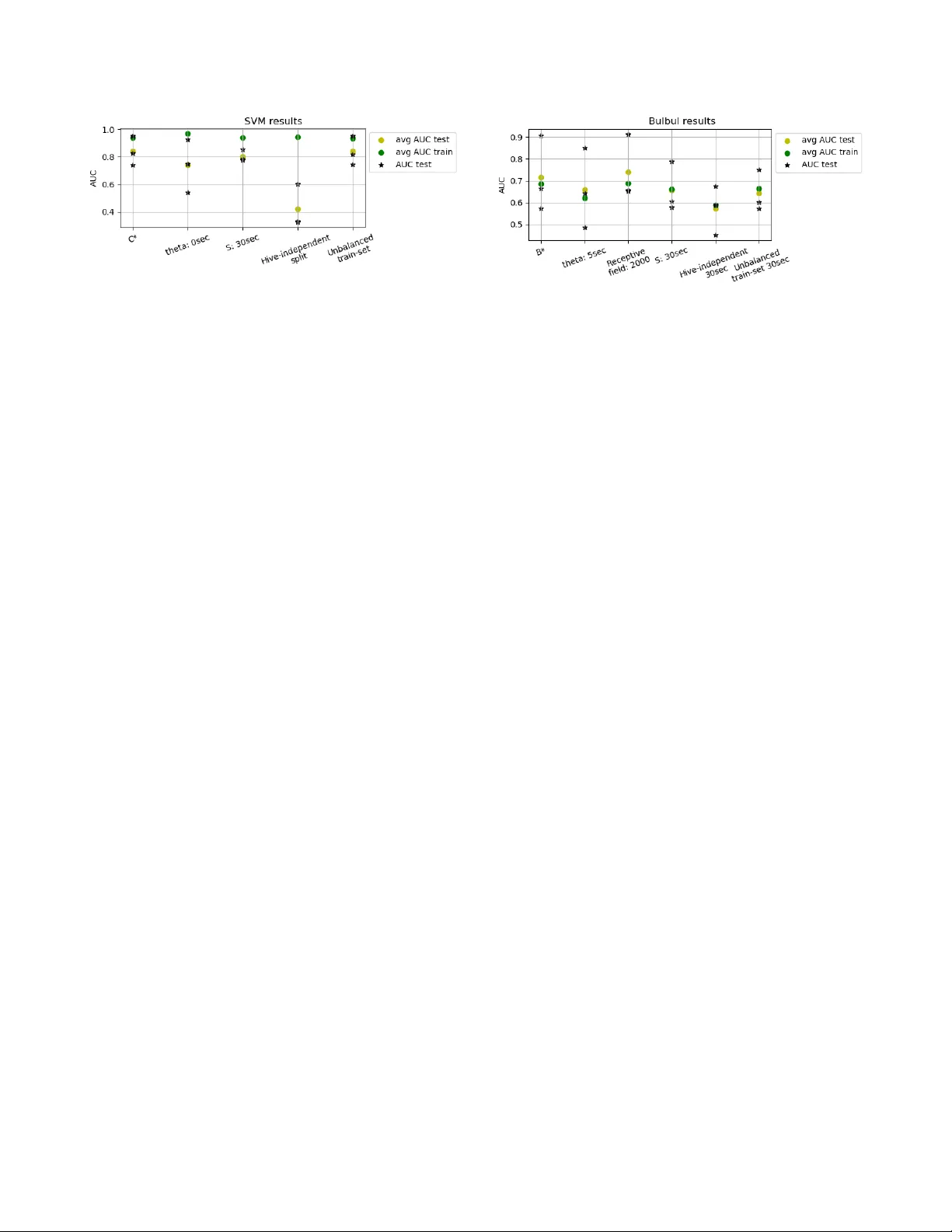
Detection and Classification of Acoustic Scenes and Events 2018 19-20 November 2018, Surre y , UK TO BEE OR NO T TO BEE: INVESTIGA TING MA CHINE LEARNING APPR O A CHES FOR BEEHIVE SOUND RECOGNITION In ˆ es Nolasco and Emmanouil Benetos School of Electronic Engineering and Computer Science, Queen Mary Uni versity of London, UK { i.dealmeidanolasco@,emmanouil.benetos@ } qmul.ac.uk ABSTRA CT In this work, we aim to explore the potential of machine learn- ing methods to the problem of beehive sound recognition. A major contribution of this work is the creation and release of annotations for a selection of beehive recordings. By experimenting with both support v ector machines and con volutional neural netw orks, we e x- plore important aspects to be considered in the de velopment of bee- hiv e sound recognition systems using machine learning approaches. Index T erms — Computational bioacoustic scene analysis, ecoacoustics, beehiv e sound recognition. 1. INTRODUCTION A significant part of computational sound scene analysis research in volv es the dev elopment of methods for automatic analysis of sounds in natural environments. This area of research has close links with the field of bioacoustics and has se veral applications, including automatic biodiv ersity assessment and automatic animal welfare monitoring [1]. Within the context of computational bioa- coustic scene analysis , the de velopment of technologies for auto- mated beehi ve monitoring has the potential to revolutionise the bee- keeping profession, with benefits including b ut not limited to a re- duction of manual inspections, distant monitoring of bee popula- tions, and by rapidly identifying phenomena related to the natural cycle of the beehi ve (e.g. queen missing, bee swarming). In particular , sound plays a central role towards the dev elop- ment of such technologies for automated beehiv e monitoring. In [2, 3], the authors give a thorough description of bee sounds and their characteristics. In short, the sound of a beehive is a mixture of the individual contributions of sounds produced by each bee of the colony . This mixture is percei ved as a dense, continuous, lo w- frequency b uzz. The first step tow ards the creation of audio-based beehi ve mon- itoring technologies is to create systems that are able to recognise bee sounds and discriminate them from other sounds that might be captured. These non-bee sounds will usually be related with the en vironment and e vents occurring in the hive’ s surroundings and can be as varied as urban sounds, animals, rain, or maintenance sounds. Thus, the aim of this work is to automatically detect sounds produced by bees, distinguishing them from external non-related sounds, given audio recordings captured inside beehi ves. One as- pect that appears useful to differentiate between both classes is that the majority of non-beehiv e sounds can be of a short duration when compared with beehiv e sounds. This work was supported by UK EPSRC grant EP/R01891X/1 and a UK RAEng Research Fellowship (RF/128). Related works in beehive sound analysis generally use heavy data pre-processing, hand-crafted features and domain knowledge to clean the recordings and come up with useful representations for beehiv e audio signals. In [4], the authors apply at a first stage a Butterworth filter with cut-of f frequencies of 100 Hz and 2000 Hz in order to filter the acoustic signal and remove all sounds of fre- quencies expected not to be in the bee sound class. In [5], besides the use of se veral filtering techniques, the authors propose the use of Mel-frequency cepstral coefficients (MFCCs) as features to rep- resent beehi ve sounds, inspired by speech processing research. The work of [6] is directly rele vant to this paper , since a classification is performed to clean the recordings from e xternal sounds. This task is set up to distinguish between 3 classes: beehiv e sounds, en viron- mental sounds and cricket sounds. Howe ver , denoising techniques and hand-crafted features are still applied, including W avelet trans- forms and features such as MFCCs, chroma and spectral contrast. Machine learning methods, and in particular deep learning methods, can decrease up to a point the amount of handcrafted fea- tures and domain kno wledge which can be responsible for intro- ducing bias and limiting the modelling capabilities of sound recog- nition methods. In [7], deep neural networks (DNNs) and con volu- tional neural networks (CNNs) are used to automatically detect the presence of mosquitoes in a noisy en vironment, although the pro- posed methodology disre gards the long duration characteristics of mosquito sounds. The work of [8] tackles the problem of detecting the presence of birds from audio as part of the 2017 Bird Audio De- tection challenge 1 . The proposed method, Bulbul , is a combination of deep learning methods also relying on data augmentation. Given that Bulb ul was the challenge submission that produced the best results, it became the baseline method for the DCASE 2018 Bird Audio Detection task 2 . In the context of environmental sound scene analysis, it is shown in [9] that DNNs hav e good performance when compared to shallower methods such as Gaussian mixture models (GMMs). Howe ver the authors also stress that the use of temporal methods such as recurrent neural netw orks (RNNs) does not im- prov e classification in this conte xt, which they justify with the char- acteristic of en vironmental sounds as not having strong temporal dependencies and being rather non-predictiv e and random. In this work, we aim to explore the potential of machine learn- ing methods to the problem of beehiv e sound recognition, as a first step to wards the creation of audio-based beehiv e monitoring sys- tems. A core problem when using supervised machine learning methods is the large amount of labelled data needed. A major con- tribution of this w ork is the creation and release of annotations for a 1 http://machine- listening.eecs.qmul.ac.uk/ bird- audio- detection- challenge/ 2 http://dcase.community/challenge2018/ task- bird- audio- detection Detection and Classification of Acoustic Scenes and Events 2018 19-20 November 2018, Surre y , UK selection of recordings from the Open Source Beehive project [10] and for a part of the NU-Hive project dataset [11]. The annotated data is used in experiments using support vector machines (SVMs) and a CNN-based approach by adapting the Bulbul implementation [8]. The results presented are indicativ e of the important aspects to be considered in the de velopment of machine learning-based bee- hiv e sound recognition systems. The outline of the paper is as follo ws. In Section 2 we de- scribe the data and the annotation procedure. Section 3 describes the methods applied; Section 4 presents the experiments performed, the ev aluation metrics, and results. Finally , Section 5 concludes the paper and provides directions for future research. 2. DA T A ANNO T A TION The main issue of posing the problem of automatic recognition of beehiv e sounds as a classification problem is the need for annotated data. In this case we need examples of pure beehive sounds and examples of external sounds as the y occur in the recordings made inside the beehiv es, so that the methods can learn their character- istics and map them to the corresponding labels. Giv en the lack of labelled data for this task, a major effort of dev eloping such a dataset is undertaken here. The resulting dataset is based on a se- lected set of recordings acquired in the context of two projects: the Open Source Beehive (OSBH) project [10] and the NU-Hive project [11]. The main goal of both projects is to dev elop beehiv e monitor- ing systems capable of identifying and predicting certain e vents and states of the hive that are of interest to beekeepers. Among many different variables that can be measured and that help the recogni- tion of dif ferent states of the hi ve, the analysis and use of the sound the bees produce is a big focus for both projects. The recordings from the OSBH project [10] were acquired through a citizen science initiativ e which asked members of the gen- eral public to record the sound from their beehives together with the registering of the hive state at the moment. Because of the am- ateur and collaborativ e nature of this project, the recordings from the OSBH project present great div ersity due to the very dif ferent conditions in which the signals were acquired: dif ferent recording devices used, dif ferent environments where the hiv es were placed, and ev en different position for the microphones inside the hi ve. This variety of settings makes this dataset a very interesting tool to help ev aluate and challenge the methods developed. The NU-Hiv e project [11] is a comprehensi ve ef fort of data ac- quisition, concerning not only sound, b ut a vast amount of vari- ables that will allow the study of bee behaviours. Contrary to the OSBH project recordings, the recordings from the NU-Hi ve project are from a much more controlled and homogeneous en vironment. Here the occurring e xternal sounds are mainly traf fic, honks and birds. The annotation procedure consists in listening the selected recordings and marking the onset and offset of e very sound that could not be recognised as a beehiv e sound. The recognition of external sounds is based primarily on the perceived heard sounds, but a visual aid is also used by visualising the log-mel-frequency spectrum of the signal. All the above are functionalities offered by Sonic V isualiser 3 , which was used by two volunteers that are neither bee-specialists nor specially trained in sound annotation tasks. By marking these pairs of instances corresponding to the beginning and end of external sound periods, we are able to get the whole record- 3 http://sonicvisualiser.org/ Figure 1: Example of the annotation procedure for one audio file. ing labelled into Bee and noBee intervals. The noBee intervals refer to periods where an external sound can be perceiv ed (superimposed to the bee sounds). An e xample of this process is shown in Fig. 1. The whole annotated dataset consists of 78 recordings of vary- ing lengths which make up for a total duration of approximately 12 hours of which 25% is annotated as noBee events. About 60% of the recordings are from the NU-Hive dataset and represent 2 hives, the remaining are recordings from the OSBH dataset and 6 differ - ent hives. The recorded hi ves are from 3 regions: North America, Australia and Europe. The annotated dataset 4 and auxiliary Python code 5 are publicly av ailable. 3. METHODS 3.1. Preprocessing The audio recordings are processed at a 22050 Hz sample rate, and are segmented in blocks of predefined lengths. Segments smaller than the defined block length hav e their length normalised by re- peating the audio signal until the block length is reached. For each block a label is assigned based on the existing annotations. A label Bee is assigned if the entirety of the segment does not contain nor ov erlap any external sound interval. Similarly , the label noBee is assigned if at least a part of the segment contains an external sound ev ent. Finally , the training data is artificially balanced by randomly duplicating segments of the class less represented. In order to ev aluate the impact of the length of external sounds, we explore different threshold v alues ( Θ ) for the minimum duration of external sounds to be included in the annotations. 3.2. SVM classifier W e first create a system for beehiv e sound recognition using a sup- port vector machine (SVM) classifier . In order to gain insight on which features, normalisation strategies and other classifier param- eters are promising to use in this problem, we explore a set of com- binations of the three on the SVM classifier, detailed in Section 4.3. T wo types of features are extracted for use with the SVM: 20 Mel- frequency cepstral coef ficients (MFCCs) and Mel spectra [12], the latter with 80 and 64 number of bands. The spectra are computed with a window size of 2048 samples and hop size of 512 samples. 4 https://zenodo.org/record/1321278#.W2XswdJKjIU 5 https://github.com/madzimia/Audio_based_ identification_beehive_states Detection and Classification of Acoustic Scenes and Events 2018 19-20 November 2018, Surre y , UK 3.3. CNN classifier For the deep learning approach we explore the application of the Bulbul CNN implementation [8] as modified for the DCASE 2018 Bird Audio Detection task. The choice of this implementation for a first experiment using a deep learning approach is due to both its promising results achieved in the Bird Audio Detection Challenge, but also because the original problem for which the Bulbul system was de veloped poses similar challenges as the ones we face. In this implementation, Mel spectra with 80 bands are com- puted using a window size of 1024 samples and a hop size of 315 samples. Additionally , these spectra are normalised by subtracting their mean over time. The network consists of four conv olution lay- ers (two layers of 16 filters of size 3 × 3 and two layers of 16 filters of size 3 × 1 ) with pooling, followed by three dense layers (256 units, 32 units and 1 unit). All layers use a leaky rectifier as acti va- tion function with the exception of the output layer which uses the sigmoid function. Data augmentation is also employed, which includes shifting the training examples periodically in time, and applying random pitch shifting of up to 1 mel band. Dropout of 50% is applied to the last three layers during training. 4. EV ALU A TION 4.1. Experimental setup Giv en the diversity of the data av ailable we are interested in ev alu- ating ho w well the classifiers are able to generalise to dif ferent data. Thus, besides random splitting between train and test sets, we im- plement a “hiv e-independent” splitting scheme. This means having training samples belonging only to certain hives, and testing using samples from other , unseen hiv es. For both schemes a test size of 5% is used (5% of the total number of se gments in the case of the random split scheme or 5% of the number of hiv es in the hiv e-independent splitting scheme). When applying the SVM classifier , all remaining data is used in a single training set. For the b ulbul implementation, in order to mimic the original cross validation scheme, where a model is trained in each set and validated on the others, the remaining data (95%) is further split in half between two sets. The training of the Bulbul netw ork is done by stochastic gradi- ent descent optimisation on a mini-batch of 20 input samples of size 1000 frames by 80 Mel-frequencies (receptive field), and through 100 epochs. The training samples are organised in tw o sets, and the resulting two trained models are ensembled to generate the predic- tions in the test set. The prediction for a single sample is obtained by a veraging the netw ork output predictions of the non-ov erlapping 1000 frame excerpts that constitute the whole input sample. 4.2. Evaluation Metrics The results of each experiment are ev aluated using the area under the curve score (A UC) [13]. Each e xperiment is run three times following the same setup and parameters, and we report the results on each run and the av erage of the three. The results on the training set are also reported. 4.3. SVM Experiments As mentioned in Section 3, in this approach a combination of the below parameters is e valuated: SVM kernels: RBF , linear , and 3 rd order polynomial. Featur es: µ and σ of: 20 MFCCs, the ∆ of 20 MFCCs and of the ∆∆ of 20 MFCCs; µ and σ of: Mel-spectra and ∆ of Mel- spectra with 64 or 80 bands; µ and σ of: log Mel-spectra and ∆ of log Mel-spectra with 64 or 80 bands; Normalisation strategies: no normalisation, normalisation by maximum value per recording, by maximum value in dataset, z-score normalisation at recording le vel, and z-score normal- isation at dataset lev el. Segment size ( S ): 30 seconds and 60 seconds. Threshold Θ : 0 seconds and 5 seconds. Split modes: Hive-independent and Random split Combining these parameters and ev aluating the results of each combination leads us to define the optimal set of parameters (C*). In order to thoroughly ev aluate the classifier, e xperiments using C* are compared against specific parameter changes: (a) different value of threshold Θ ; (b) dif ferent segment size S; (c) Hive-independent split of the data to determine the generalisation capability to unseen hiv es; (d) Unbalanced dataset to determine the robustness of the classifier regarding unbalanced classes. 4.4. CNN Experiments Where possible, parallel experiments to the SVM approach are set up here. As baseline parameters (B*), we use the follo wing: Featur es: 80 Mel-band spectra Receptive field: 1000 frames Number of training epochs: 100 Batch size: 20 Experiments with changes to these parameters are: (a) different values of Θ , to determine if the classifier can learn to reject only external sounds with long durations; (b) dif ferent v alues of segment size S ; (c) Hive-independent split of data, to determine the gener- alisation capability of the classifier to unseen hiv es; (d) unbalanced dataset, to determine how the classifier can cope with this aspect; (e) larger recepti ve fields, to determine if the classifier can exploit the larger conte xt of the input samples. 4.5. SVM Results The resulting average A UC scores for the test and training set of the 3 runs of each experiment are shown in Fig. 2. From the 1 st experiment we infer that the highest average A UC score in test sets is achieved when we use the follo wing combination of parameters (C*): features as the µ and σ of the v alue, the ∆ and the ∆∆ of 20 MFCCs, not considering the first coef ficient; S of 60 seconds, Θ of 5 seconds and not using any of the normalisation strategies defined. Fig. 2 [ Θ : 0sec] shows the A UC results for the experiment us- ing the C* parameters but changing Θ from 5 to 0 seconds. These show primarily that the classifier is not performing in a consistent way , which may indicate a strong dependency on the individual in- stances in which it is being tested and trained. Also the larger differ - ence between the scores in the train and test sets indicate overfitting to the training examples. Using the smallest value for Θ means that we pro vide to the classifier samples from which their label is defined based on what can be v ery short duration e vents. It is there- fore expected that the classifier struggles to distinguish the classes. Detection and Classification of Acoustic Scenes and Events 2018 19-20 November 2018, Surre y , UK Figure 2: SVM results on the test set for each of the 3 runs ( ? ), using the A UC score. The • and • represent the average A UC score of the 3 runs in both train and test sets respectiv ely . By running the classifier with C* parameters but with segment size changed from 60 to 30 seconds (Fig. 2 [ S : 30sec] ), we can observe a decrease in both A UC in the train and test sets. These results affirm the idea that, given the long-term aspect of the beehi ve sounds, if we pro vide more context to the classifier , it will be better at distinguishing between the two classes of sounds. In Fig. 2 [Hive-independent split] , the classifier is run on 3 sets of data split using the hive-independent splitting scheme. The results clearly show the inability of the classifier to generalise to unseen hiv es. Fig. 2 [Unbalanced train-set] shows the results of running the classifier in the same sets as experiment C*, b ut not replicating sam- ples to artificially balance the sets. Comparing the two, they are almost identical which makes sense for SVMs since when data bal- ancing is performed by simple data duplication, the new points are all in locations where data points already existed, therefore these do not influence the decision boundary found by the SVM. 4.6. CNN Results The resulting average A UC scores for the test and training sets for the 3 runs of each experiment are shown in Fig. 3. The first experi- ment determined that the best average A UC in the test sets of the 3 runs is achie ved when we use the baseline parameters defined in 4.4 plus the follo wing parameters: S of 60 seconds and Θ of 0 seconds. The best results are shown in Fig. 3 [B*] . Regarding the values of Θ , Fig. 3 [ Θ : 5sec] shows that using a larger Θ is detrimental to performance. This may be explained by the fact that the Bulbul system was specifically designed for the de- tection of bird sounds, which are mainly short duration ev ents, and thus struggles to identify longer ev ents like traf fic and rain sounds. The experiment to e valuate if providing more conte xt to the net- work impro ves performance is done by changing the recepti ve field from 1000 ( ∼ 14 seconds) to 2000 ( ∼ 30 seconds). In Fig. 3 [Re- ceptive field: 2000] , the results show that indeed more context is particularly useful in the context of this problem. This is also con- sistent with the results from the SVM approach. The role of S in the CNN approach is different from the SVM one. Here, a larger segment size does not imply that larger samples with more context are gi ven to the classifier , since this is controlled by the receptive field of the network. Howe ver , given that predic- tion is done for a whole segment by a veraging the predictions for each frame, using larger segments leads to introducing more con- text. Confirming the results regarding the need for more context, Fig. 3 [S: 30sec] shows that using a smaller segment size results in Figure 3: Results for the Bulb ul CNN using the A UC score, for each of the 3 runs ( ? ). The • and • represent the average A UC score of the 3 runs in both train and test sets respectiv ely . slightly worse predictions than using a larger segment size ( S : 60 seconds, shown in Fig. 3 [B*] ). Fig. 3 [Hiv e-independent 30sec] sho ws the results when using a hiv e-independent splitting scheme in a 30 second segment size data. Comparing this with the results in Fig. 3 [S: 30sec] , the lack of generalisation capacity to unseen hiv es is also evident here, al- though, compared with the SVM approach, the results seem to be slightly better and less overfitting occurs which may indicate better generalisation capabilities for the CNN. Fig. 3 [Unbalanced train-set 30sec] shows the results of not doing data balancing on the 30 second segment data. When com- paring with Fig. 3 [S: 30sec] , the results indicate that data balancing should be considered when training this CNN. 5. CONCLUSIONS In this work we allocate a major effort for the creation of an anno- tated dataset for beehi ve sound recognition where machine learning approaches can be used. Ho wev er , the annotation procedure can be improv ed for future additions to this dataset: ideally annotations should be performed by specialists which label overlapping sets of data so that the annotations are subject to peer validation. Finally the main critique to the annotations could be that they are the most important source of human bias introduced in this work. Although the scores achiev ed by the CNN implementation fail to achiev e the le vel of the SVM approach, results are indicati ve of the important aspects to be considered when de veloping neural net- works to tackle this unique problem. Mainly , the importance of providing samples with large context, the amount of training data, and finally due to the incapacity of both approaches to generalise to different hi ves, the one constraint would be to train systems in the same hiv es where they are going to be used. W e consider that this work can be a first step in a pipeline of beehi ve monitoring sys- tems, which we think will hav e an important role in the future of bee keeping. Finally , we expect that this work and the release of the an- notated dataset to further moti v ate research in this topic, and more broadly in the intersection of machine learning and bioacoustics. 6. A CKNO WLEDGEMENT W e would like to thank the authors of the NU-Hive project for cre- ating such complete dataset and making it av ailable for us to work with. Also a special thanks to Ermelinda Almeida for her effort and dedication on annotating the data. Detection and Classification of Acoustic Scenes and Events 2018 19-20 November 2018, Surre y , UK 7. REFERENCES [1] D. Stowell, “Computational bioacoustic scene analysis, ” in Computational Analysis of Sound Scenes and Events , T . V ir- tanen, M. D. Plumbley , and D. P . W . Ellis, Eds. Springer , 2018, pp. 303–333. [2] M. Bencsik, J. Bencsik, M. Baxter, A. Lucian, J. Romieu, and M. Millet, “Identification of the honey bee swarming process by analysing the time course of hiv e vibrations, ” Computers and Electr onics in Agricultur e , vol. 76, no. 1, pp. 44–50, 2011. [3] A. Zacepins, A. Kviesis, and E. Stalidzans, “Remote detec- tion of the swarming of honey bee colonies by single-point temperature monitoring, ” Biosystems Engineering , vol. 148, pp. 76–80, 2016. [4] S. Ferrari, M. Silva, M. Guarino, and D. Berckmans, “Moni- toring of swarming sounds in bee hives for early detection of the swarming period, ” Computers and Electronics in Agricul- tur e , vol. 64, no. 1, pp. 72–77, 2008. [5] A. Robles-Guerrero and T . Saucedo-Anaya, “Frequency anal- ysis of honey bee b uzz for automatic recognition of health sta- tus: A preliminary study , ” Resear ch in Computing Science , vol. 142, no. 2017, pp. 89–98, 1870. [6] P . Amlathe, “Standard machine learning techniques in audio beehiv e monitoring: Classification of audio samples with lo- gistic regression, K-nearest neighbor, random forest and sup- port v ector machine, ” Master’ s thesis, Utah State Uni versity , 2018. [7] I. Kiskin, P . Bernardo, T . W indebank, D. Zilli, and M. L. May , “Mosquito detection with neural networks: The buzz of deep learning, ” ArXiv e-prints , pp. 1–16, 2017, [8] T . Grill and J. Schl ¨ uter , “T wo conv olutional neural netw orks for bird detection in audio signals, ” in 25th Eur opean Signal Pr ocessing Conference (EUSIPCO) , 2017, pp. 1764–1768. [9] J. Li, W . Dai, F . Metze, S. Qu, and S. Das, “ A comparison of deep learning methods for en vironmental sound detection, ” in IEEE International Confer ence on Acoustics, Speech and Signal Pr ocessing (ICASSP) , Mar . 2017, pp. 126–130. [10] “Open Source Beehiv es Project, ” https://www .osbeehi ves. com/. [11] S. Cecchi, A. T erenzi, S. Orcioni, P . Riolo, S. Ruschioni, and N. Isidoro, “ A preliminary study of sounds emitted by honey bees in a beehiv e, ” in Audio Engineering Society Con vention 144 , 2018. [12] R. Serizel, V . Bisot, S. Essid, and G. Richard, “ Acoustic fea- tures for environmental sound analysis, ” in Computational Analysis of Sound Scenes and Events , T . V irtanen, M. D. Plumbley , and D. P . W . Ellis, Eds. Springer, 2018, pp. 13–40. [13] A. Mesaros, T . Heittola, and D.Ellis, “Datasets and ev al- uation, ” in Computational Analysis of Sound Scenes and Events , T . V irtanen, M. D. Plumbley , and D. P . W . Ellis, Eds. Springer , 2018, pp. 13–40.