Optimal measures and Markov transition kernels

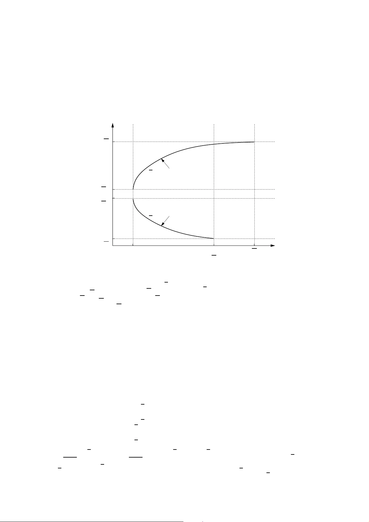
The final publ ication is av ail able at www .springe rlink.co m In J Glob Optim DOI: 10.10 07/s1 0898- 012-9851-1 Optimal measures and Markov transition kernels ∗ Roman V . Bela vkin Draft of 29 Nov ember 2011 Abstract W e study optimal solu tions to an ab stract o ptimization p roblem for measu res, wh ich is a gener alization of classical v ariational problem s in informa tion theor y and statistical physics. In the classical prob lems, in formatio n and relative en tropy are defined using the Kullback-Leib ler d iv ergence, and for this reason op timal measures belo ng to a one- parameter exponential f amily . Measu res within such a family ha ve t he prop erty of mutual absolute continu ity . Here w e show that this prop erty characterizes other families of op ti- mal positiv e mea sures if a functional representin g inform ation has a strictly con vex dual. Mutual abso lute continuity of optimal prob ability measures allows us to strictly separate deterministic and no n-determ inistic Mar kov tran sition kernels, w hich play an important role in theories of decisions, estimation, contro l, commun ication and comp utation. W e show that d eterministic tr ansitions are strictly sub-op timal, u nless in formatio n resource with a strictly conve x du al is unconstrain ed. For illustration, we construct an example where, unlike non-determ inistic, any deter ministic kernel either has negativ ely infinite expected utility (unboun ded expected error) or commu nicates infinite inform ation. 1 Introd uction This work was motiv ated by the f act that probabi lity measures within an expon ential f amily , which are solution s to va riation al prob lems of information theo ry and statistic al physics , are mutually absolutely contin uous. Thus, we beg in by clarifying and discussing this property in the simplest setting . L et Ω be a fi nite set, and let x : Ω → R be a real function. Consider the family { y β } x of real function s y β : Ω → R , inde xed by β ≥ 0: y β ( ω ) = e β x ( ω ) y 0 ( ω ) , y 0 ( ω ) ≥ 0 (1) The elements of { y β } x repres ent one-parameter expone ntial measures y β ( E ) = ∑ ω ∈ E y β ( ω ) on Ω , and normalized elemen ts P β ( ω ) = y β ( ω ) / y β ( Ω ) are the cor respon ding ex ponential probab ility measures. Of cou rse, expo nential measures can be defined on an infinite set, for exa mple, as elements of the Banach space Y : = M ( Ω , R , k · k 1 ) of real Radon measu res on a locally compac t space Ω [11]. In this case, x and e x are elemen ts of the normed algebra X : = C c ( Ω , R , k · k ∞ ) of continuou s funct ions with compact support in Ω . As will be clarified later , Y can be consid ered not only a s the dual of X , but also as a module ove r alg ebra X , whic h exp lains the definition of an ex ponen tial family (1) as multip licatio n of y 0 ∈ Y by elemen ts of X . Furthermor e, for some y 0 , e xponential m easure s are finite ev en if fun ction x is not contin uous, has non-compact support and unbounded . A similar constr uction can be m ade in the case when X is a non- commutati ve ∗ -algebr a, such as the algebra of compact Hermitian ∗ This work was sup ported by EPSR C gran t EP/H031936/1. operat ors on a separable Hilbert spa ce used in qu antum pro bability theory . Howe ver , qua ntum exp onent ial measures can be defined in di f ferent ways, such as y β : = exp ( β x + ln y 0 ) or y β : = y 1 / 2 0 exp ( β x ) y 1 / 2 0 , which are not equi val ent. One prope rty that characterize s all these expone ntial measures is that elements within a family are mutuall y ab solute ly continu ous. W e remin d that measur e y is absolutely cont inuou s with respect to measure z , if z ( E ) = 0 implies y ( E ) = 0 for all E in the σ -ring of subsets of Ω . Mutual abso lute continuity is the case when the implic ation holds in both directions . It is easy to see from equation (1) that exponent ial measur es within one family hav e exactly the same supp ort and are mutually absolu tely continuou s. This property is particul arly important, when measures are consid ered on a compos ite system, such as a direct produ ct of two sets Ω = A × B . Normalized measur es on such Ω are joint pr obabi lity measures P ( A × B ) uniquely defining condition al probabil ities P ( A | B ) (i.e. Marko v transition kerne ls). Observ e now that if P ( A × B ) and P ( A ) P ( B ) (produc t of mar ginals) are mutually absolut ely continuous , then P ( a | b ) > 0 for all a ∈ A s uch t hat P ( a ) > 0. Conditional p robability with th is prop erty is no n- determin istic, because sev eral elements a ∈ A can be in the ‘imag e’ of b ∈ B . Clearl y , all joint probab ility measures within an exp onent ial famil y define such non-determin istic trans ition ker nels. Another , perhaps the most important, prop erty of exp onential fa m ilies is that they are, in a certain sense, optimal. It is well-kno wn in mathematica l statistics that the lower bound for the varian ce of the unbiased estimator of an unkno wn parameter , defined by the Rao-Cramer inequa lity , is attained if and only if the probability distrib ution is a member of an expone ntial family [1 3, 31]. In statistical physics, it is kno wn that exponen tial distrib utions ( i.e. Boltzmann or Gibbs distrib utions) maximize entropy of a thermodyn amical system under a constr aint on ener gy [17]. In infor mation theory , expon ential transition ker nels are kno wn to maximize a chann el capacity [33, 34, 35], and they are used in some randomized optimization techniques (e.g. [20]) as well as variou s machine learning algorithms [39]. A one-par ameter e xponential family has been studied in informati on geometry , and it was shown to be a Banach space with an Orlicz norm [30 ]. Similar construc tions hav e been considered in quantum probability [10, 36]. Optimality of expo nential f amilies of measures on one hand and their mutual absolute contin uity on the other is a particu larly intere sting combin ation, becau se it seems that for the first time we ha ve an opt imality criterio n, with resp ect to which all deterministi c transitions between el ements of a c omposite system are stri ctly sub-o ptimal. This appe ars to ha ve impor - tance not only for information and communication theories, but also for theori es of computa- tional a nd algo rithmic comple xity , because Marko v transitio n kernels can be u sed to repre sent v arious input-o utput systems, includ ing computation al syste m s and algorithms. Thus, under- standi ng the rela tion between mutual absolu te continu ity w ithin some famil ies of measures and their optimal ity was the main motiv ation for this work. It is w ell-kn o w n, and will be reminded later in this pap er , that a one-paramete r e xpo- nentia l family of probabili ty measur es is the so lution to a v ariatio nal problem of minimizing Kullb ack-Leib ler (KL) di ver gence [23] of one pro babili ty measure from another subject to a constr aint on the e xpected v alue. In fact, the logarithmic fun ction, whic h ap pears in the defini - tion of the KL-di ver gence, is precisely the reason why the exp onent ial function appears in the soluti ons. Ho weve r , mutu al abso lute con tinuity , which f or compo site sys tems implies the non - determin istic property of conditio nal probabili ties, is not exclus i ve to familie s of expone ntial measures . Indeed, geometrical ly , this property simply means that measures are in the inte- rior of the same positi ve cone, defined by the ir common support. Thus, our method is based on a generalizati on of the abo ve mentio ned v ariationa l probl em by relaxing the definition of 2 informat ion and then employ ing geometric analys is of its solutions . In the ne xt secti on, we introduce th e notation, de fine the generalize d optimizati on problem and recall some basic relev ant facts. An abstract informat ion resource will be repres ented by a clo sed functi onal F : Y → R ∪ { ∞ } , defined on the space Y of measures , and such that its v alues F ( y ) can be associate d with valu es I ( y , y 0 ) of some informat ion distance (e.g. the KL - di ver gence). In Section 3 we establish se veral properties of opt imal solu tions. In particu lar , we prov e in Proposition 3 that the optimal value function is order isomorphism puttin g infor - mation in duality with ex pected utility of an optimal system. These results are then used in Section 4 to pro ve a theor em relating mutual absol ute continuit y of optimal pos iti ve m easure s to strict con ve xity of function al F ∗ , the Legendre- Fenchel dual of F represe nting information resour ce. W e sho w that strict con ve xity of F ∗ is necessary to separ ate dif ferent varia tional proble ms by optimal m easure s, and for this reason it appea rs to be a natural minimal require- ment on info rmation, generalizi ng the additi vity axiom. Because proo f of m utual abso lute contin uity does not depend on commutati vity of algebra X , pre-dual of Y , these results apply to a genera l, non-co m mutati ve setti ng used in quantum probability and info rmation theorie s. In S ection 5, we discu ss opti mal Mark ov transition kern els (condi tional probabil ities) in the classic al (commutati ve) setting , which is done for simplicit y reasons. W e shall recall sev eral fact s abou t trans ition k ernels, informat ion cap acity of memoryles s channels they repr esent an d the correspo nding v ariationa l probl ems. The main result of this section is a theorem separat - ing determinis tic and non-dete rministic k ernels. W e show how mutual absolu te continui ty of optimal Marko v transiti on kern els implies that optimal transitions are non-det erminist ic; de- terminist ic transitions are strictly subopti mal if information, understo od broadly here, is con- straine d. This result will be illustrate d by an example, where any det erministi c ker nel either has a ne gativ ely infinite expec ted utility (unbou nded expect ed error) or communicates infinite informat ion; a non-dete rministic kern el, on the other hand, can hav e both finite expecte d util- ity a nd finite inf ormation . In the e nd of the section we s hall consi der applica tions of this w ork to theories of algori thms and computatio nal comple xity . W e shal l dis cuss ho w deterministic and non-dete rministic algorithms ca n be represent ed by Marko v trans ition k ernels be tween the space of inp uts and the space of output sequen ces, and ho w constraints on the expe cted utility or complexi ty of the algori thms are related to v ariatio nal proble ms studied in this work. The paper conc ludes by a summary and discussion of the results. 2 Pr eliminaries This work i s based on a general izatio n of classica l variati onal problems of informatio n theory and statis tical physics, which can be formulated as follo ws. Let ( Ω , R ) be a measura ble set and let P ( Ω ) be the set of all Radon probab ility measures on Ω . W e denote by E p { x } the expecte d v alue of random variab le x : Ω → R with respe ct to p ∈ P ( Ω ) . An infor mation distance is a function I : P × P → R ∪ { ∞ } that is closed (lower semicon tinuou s) in each argumen t. An import ant example is the Kullback -Leibler div erge nce I K L ( p , q ) : = E p { ln ( p / q ) } [23]. W e remind that E p { x } is linear in p , and I K L ( p , q ) is con vex. The v ariational problem is formulated as follo ws: maximize (minimize) E p { x } subjec t to E p { ln ( p / q ) } ≤ λ (2) where optimizati on is ov er probabilit y measures p ∈ P . This problem can be con sidered as linear programming with an infinite number of linear constr aints, and it can be formulate d as 3 the foll o w ing con ve x progra mming problem: minimize E p { ln ( p / q ) } subject to E p { x } ≥ υ  E p { x } ≤ υ  (3) Figure 1 illustra tes the se variat ional problems on a 2-simplex of probab ility measur es over a set of three elemen ts with the uniform distrib ution q ( ω ) = 1 / 3 as the referen ce measure. q p β E p { x } ≥ υ E p { ln ( p / q ) } ≤ λ Figure 1: 2-Simplex P of probabili ty measur es over set Ω = { ω 1 , ω 2 , ω 3 } with le vel sets of exp ected utility E p { x } = υ and the Kullback -L eibler di ver gence E p { ln ( p / q ) } = λ . P roba- bility measure p β is the solution to var iation al problems (2) and (3 ). The family { p β } x of soluti ons, shown by dash ed curve, belong s to the interior of P . In optimizati on and information theories , E p { x } represents ex pected utility to be maxi- mized or e xpected cost to be minimized. In physics, it repre sents internal ener gy . Information distan ce I K L ( p , q ) is also call ed relat i ve e ntrop y , and t he inequal ity I K L ( p , q ) ≤ λ repres ents an informat ion constr aint . Depending on the domai n of definit ion of the probability measures, the information const raint may hav e dif ferent meanin gs, such as a lower boun d on entropy (i.e. irredu cible uncertai nty), partial observ ability of a rand om var iable, a co nstrain t on the amount of stati stical informati on (i.e. a number of i ndepe ndent tests, que stions or bi ts of information), on communica tion capac ity of a channel, on memory of a computat ional de vice and so on [35]. These v ariatio nal problems can also be formulated in quantum physics, where x is an element of a non- commutati ve algebra of observ ables, and p , q are quantum probabilit ies (states). As is well-kn o w n, solutions to probl ems (2) and (3) are el ements of an e xponential family of prob ability distrib utions. Before we define an appropriate general izatio n of the se prob lems, we remind some axio matic principles underpinnin g the choice of functional s. 2.1 Axioms beh ind the choice of functionals The choice of linear o bjectiv e function al E p { x } has axiomatic foun dation in game theory [2 7 ], where Ω is equ ipped with total pre-ord er . , called the pr efer ence re lation , and functio n x : Ω → R is its utili ty r epr esentat ion : ω 1 . ω 2 if and only if x ( ω 1 ) ≤ x ( ω 2 ) . Because the quot ient 4 set Ω / ∼ of a pre-order ed set with a utility function is isomorphic to a subset of the real line, it is separa ble and metrizab le by ρ ([ a ] , [ b ]) = | x ( a ) − x ( b ) | , and therefor e ev ery probability measure on the completi on of Ω / ∼ is R adon (e.g. by Ulam’ s theorem for probabilit y meas ures on Polish spac es). The set P ( Ω ) of al l clas sical probability measures o n Ω is a simplex with Dir ac meas ures δ ω comprisi ng the set ext P of its extreme points [29]. T he question that has been discussed ext ensi vely is: H o w to extend pre-o rder . , which was defined on Ω ≡ ext P , to the whole P ? It was sho wn in [27] that linear (or af fine) functiona l E p { x } is the only functio nal that makes the exte nded pre-o rder ( P , . ) compati ble with the vector spa ce structu re of Y ⊃ P and Archimedian. W e remind that for the correspon ding pre -order ( Y , . ) ⊃ ( P , . ) this is defined by the axio m s: 1. q . p implies q + r . p + r and α q . α p for all r ∈ Y and α ≥ 0. 2. nq . p for all n ∈ N implies q . 0. In this paper we shall follo w this formalis m assuming tha t the obj ecti ve functio nal is linea r . W e note that non-li nearit y may arise in certain dynamical systems, where x may change w ith time, but this will not be consi dered in this work, becaus e our focus is on optimizatio n prob- lems with respect to some fixe d prefere nce relation . or util ity x on Ω . A non-commuta ti ve (quant um) analogu e of a utility fun ction was gi ven in [7] by a H ermitian oper ator x on a sep a- rable Hilbert space (an observ able) with its real spectrum representin g a total pre-order on its eigen states. The p rincip al dif ference with th e cla ssical theo ry is the existence of incompatibl e (non-c ommutati ve) utility operators. As mentio ned earlier , information constrain ts may be related to dif ferent phenomena (e.g. uncert ainty , observ ability , statist ical data, communication capacity , memory , etc). H o we ver , in information theo ry they often ha ve been represente d by f unctio nals, such as relati ve entro py or Shannon informati on, which are defined using the Kullback -Leibler div er gence I K L . Its choice i s also ba sed on a number of axi oms [14, 19, 33], suc h as additi vity: I K L ( p 1 p 2 , q 1 q 2 ) = I K L ( p 1 , q 1 ) + I K L ( p 2 , q 2 ) . In fact, this axiom is precisel y the reason why the lo garithm func tion appear s in its definition (i.e. as homomorp hism between multiplic ati ve and additi ve groups of R ). There is, ho wev er , an ab undan ce of oth er infor mation distances and metrics, such as the Hellinge r distance , total v ariation and the Fisher metrics. Although they often fail to ha ve a proper statisti cal interpretatio n [12], there has been a rene wed interest in using diff erent informat ion distance s and contrast functions in applicatio ns to compare distrib utions (e.g. see [4, 6, 26]). For rea sons outlined above , we shall generali ze problems (2) and (3) by considerin g an abstra ct informatio n dist ance or resource, which will be used to define a subs et of feasi ble soluti ons. In additio n, we shall no t restric t the problems to normalized measure s, which mak es the expos ition a lot simpler . N ormaliza tion can be performed at a later stage. W e now define an appr opriat e algebra ic structure . 2.2 Dual al gebraic structur es Let X and Y be comple x linear spac es put in duality via bilinear form h· , ·i : X × Y → C : h x , y i = 0 , ∀ x ∈ X ⇒ y = 0 , h x , y i = 0 , ∀ y ∈ Y ⇒ x = 0 W e denote by X ♯ the algebraic dual of X , by X ′ the continuou s dual of a locally con ve x space X and by X ∗ the complete normed dual space of ( X , k · k ) . The same notation appl ies to 5 dual space s of Y . The results will be deri ved usin g only the facts that X and Y are ordered linear spaces in duality . These spac es, ho wev er , can ha ve ri cher algebr aic structures , which we briefly outlin e here. Space X is closed und er an associati ve, but general ly non-commutati ve binar y operatio n · : X × X → X (e.g. pointwise multiplic ation or matrix multipl icatio n) and in v olution as a se lf- in ve rse, antilinear map ∗ : X → X rev ersing the multip lication orde r: ( x ∗ z ) ∗ = z ∗ x . Thus, X is a ∗ -algebra. T he set of all Hermitian elements x = x ∗ is a real subspace of X , and if ev ery x ∗ x has positi ve real spectrum, then X is called a total ∗ -algebra, in w hich the spectrum of all Hermitian elements is real. In this case, Hermitian elements x ∗ x form a pointed con ve x cone X + , gene rating X = X + − X + . The dua l space Y is clos ed under the trans posed in vo lution ∗ : Y → Y , defined by h x , y ∗ i = h x ∗ , y i ∗ . It is ordere d by a posit i ve cone Y + : = { y : h x ∗ x , y i ≥ 0 , ∀ x ∈ X } , dual of X + , and it has ord er unit y 0 ∈ Y + (also called a reference measu re), which is a strictly pos iti ve linear functi onal: h x ∗ x , y 0 i > 0 for all x 6 = 0. If the pai ring h· , ·i has the property that for each z ∈ X there exi sts a transpos ed element z ′ ∈ Y such that h zx , y i = h x , z ′ y i , then Y ⊃ X is a left (right) m odule o ver X with resp ect to the tran spose d left (right) acti on y 7→ z ′ y ( y 7→ yz ∗′∗ ) of X on Y such that ( xz ) ′ = z ′ x ′ and h x , yz ∗′∗ i = h x ∗ , z ∗′ y ∗ i ∗ = h z ∗ x ∗ , y ∗ i ∗ = h xz , y i (see [9], Appendi x). In man y pract ical cases, the pairing h· , ·i is central (or tr acial ) , so that the left and right transposi tions act identically on y 0 : z ∗′ y 0 = y 0 z ′∗ for all z ∈ X . In this case, the element z ∗′ y 0 = y 0 z ′∗ ∈ Y can be identified with a complex conjug ation of z ∈ X . T wo pri mary exampl es of a total ∗ -algebra X , which are important in this work , are the commutati ve algebra C c ( Ω , C , k · k ∞ ) of continuous fu nctions with compact support in a l ocally compact topolog ical space Ω and the non-commutati ve algeb ra C c ( H , C , k · k ∞ ) of compact Hermitian operato rs on a separable Hilbert space H . The correspo nding example s of dual space Y = X ∗ are the Banach space M ( Ω , C , k · k 1 ) of complex signed Radon m easure s on Ω and i ts non -commutati ve generali zation M ( H , C , k · k 1 ) . Note that these e xamples o f algebra X are gen erally incomplete and c ontain only an a pproximate identity . Howe ver , by X we shall unders tand here an extended algebr a that contain s additional elements. In partic ular , X will contai n the unit elemen t 1 ∈ X such that h 1 , y i = k y k 1 if y ≥ 0 (i.e. 1 ∈ X coincides on Y + with the norm k · k 1 , which is additi ve on Y + ). Furthe rmore, because constraints in varia tional proble ms ( 2) or (3 ), o r their g eneralization s, define a p roper subs et of space Y , w e can cons ider random v ariables represe nted by elemen ts x ∈ Y ♯ that are o utside of the Bana ch space Y ∗ (e.g. unbou nded functions or operators). Belo w are three main examp les of pairing X and Y by a sum, an integral or trace: h x , y i : = ∑ Ω x ( ω ) y ( ω ) , h x , y i : = Z Ω x ( ω ) d y ( ω ) , h x , y i : = tr { xy } (4) Although the linear functio nals x ( y ) = h x , y i are generally comple x-valu ed, we shall assume, without furth er mentionin g, that h· , ·i is e valu ated on Hermitian elements x = x ∗ and y = y ∗ so that h x , y i ∈ R . In p articular , the ex pected v alue E p { x } = h x , p i ∈ R , where x is Hermit ian and p is p ositi ve. Thus, the ex pressi ons ‘maximize (minimize) x ( y ) = h x , y i ’ should be u nderst ood accord ingly as maximization or minimization of a real functional . 2.3 Generalized v aria tional pr oblems for measures Normalized non -ne gati ve measures (i.e. proba bility measures) are elements of the set: P : = { y ∈ Y : y ≥ 0 , h 1 , y i = 1 } 6 This is a weakly compa ct co n ve x set, an d the refore P = cl co ext P by the Kre in-Milman t he- orem. In the commutati ve case, P is a simplex, because each p ∈ P is uniquely represente d by extreme poin ts δ ∈ ext P [29]. In information geometry P is referred to as statistical manifold , and its topologic al propert ies ha ve been stud ied by defining diffe rent information distan ces I : P × P → R + ∪ { ∞ } [3 , 12, 3 0]. W e ca n gener alize this by con sidering informa- tion resou rce as a functional, defined for all positi ve or Hermitian element s. υ υ 0 υ 0 υ λ 0 λ λ Optimal v alues, υ = h x , y i Constrai nt valu es, λ ≥ F ( y ) x ( λ ) : = sup {h x , y i : F ( y ) ≤ λ } x ( λ ) : = inf {h x , y i : F ( y ) ≤ λ } Figure 2: Optimal va lue functions υ = x ( λ ) and υ = x ( λ ) . The value λ 0 = inf F correspon ds to υ ∈ [ υ 0 , υ 0 ] . Special valu es λ , λ of the cons traint λ ≥ F ( y ) corre spond respec tive ly to optimal v alues υ and υ . Let F : Y → R ∪ { ∞ } be a closed fun ctiona l, so that F is finite at s ome y ∈ Y , and subl e vel sets { y : F ( y ) ≤ λ } are closed in the weak topology σ ( Y , X ) for eac h λ . B ecause − ∞ is not includ ed in the definition of closed F , it is also lower -semicont inuou s [32]. W e shall assume without furth er mentionin g that the eff ecti ve domain dom F : = { y : F ( y ) < ∞ } has non-emp ty algebr aic interior . In add ition, if Y is defined ov er the fi eld of co mplex numb ers, we shall also assume that dom F contains only Hermitian elements y = y ∗ (e.g. dom F ⊆ Y + ). V ariatio nal problems (2) and (3) are generalize d by consid ering all, not necessa rily po si- ti ve or normalized measures , and by using an y closed func tional F to define an informatio n resour ce. The optimal v alues achie ved by solutions to these problems are defined by the fol- lo wing optimal value function s : x ( λ ) : = sup {h x , y i : F ( y ) ≤ λ } (5) x ( λ ) : = inf {h x , y i : F ( y ) ≤ λ } (6) x − 1 ( υ ) : = inf { F ( y ) : h x , y i ≥ υ } (7) x − 1 ( υ ) : = inf { F ( y ) : h x , y i ≤ υ } (8) W e define x ( λ ) : = − ∞ , if λ < inf F , and x ( ∞ ) : = lim x ( λ ) as λ → ∞ . Observ e that x ( λ ) = − ( − x )( λ ) and x − 1 ( υ ) = ( − x ) − 1 ( − υ ) . Thus, it is suf ficient to study only the properties of x ( λ ) . Figure 2 dep icts schematically the optimal va lue functions x ( λ ) and x ( λ ) . It is clear 7 from the definition that x ( λ ) is a non-decrea sing ext ended real function , and x ( λ ) is non- increa sing. It will be sho w n also in the nex t section that x ( λ ) is conca ve, and x ( λ ) is con ve x (Proposi tion 3). Because sets { y : F ( y ) ≤ λ } may b e unbalance d and unbounde d, the functions may not be reflections of each o ther in th e sense th at x ( λ ) − υ 0 6 = υ 0 − x ( λ ) for all υ 0 , an d on e or both functio ns can be empty . The definition of the optimal value func tions (5)–(8) in terms of funct ional F ( y ) of one v ariable , unlik e information distance I ( y , y 0 ) , allo ws for consider ing the case when inf F is not achie ved at any y 0 ∈ Y . In addition to λ 0 : = inf F , we define t wo special v alues λ and λ of func tional F as follo w s: x ( λ ) : = sup {h x , y i : y ∈ dom F } , x ( λ ) : = inf {h x , y i : y ∈ dom F } (9) Thus, problems of maximization or minimization o f x ( y ) = h x , y i subjec t to co nstrai nts F ( y ) ≤ λ or F ( y ) ≤ λ respec ti vely are equiv alent to unc onstra ined problems on dom F . The corre- spond ing optimal val ues are denot ed υ = x ( λ ) and υ = x ( λ ) , as shown on Figure 2. The reason for defining these valu es is that generally λ ≤ ∞ , λ ≤ ∞ and λ 6 = λ (see Figure 2). Solution s to unconstra ined proble ms may correspond to lar ge, possibly infinite valu es λ or λ , and therefore they can be considered unfeasible . Subsets of feasib le solutions will be defined by cons traint s F ( y ) ≤ λ < λ or F ( y ) ≤ λ < λ . In addit ion, we define the follo wing special val ues: υ 0 : = lim λ ↓ inf F sup {h x , y i : F ( y ) ≤ λ } , υ 0 : = lim λ ↓ inf F inf {h x , y i : F ( y ) ≤ λ } (10) If there exists a set ∂ F ∗ ( 0 ) ⊂ dom F such tha t inf F = F ( y 0 ) for all y 0 ∈ ∂ F ∗ ( 0 ) , then υ 0 = sup {h x , y 0 i : y 0 ∈ ∂ F ∗ ( 0 ) } and υ 0 = inf {h x , y 0 i : y 0 ∈ ∂ F ∗ ( 0 ) } . If y 0 is uniqu e, then υ 0 = υ 0 ; otherwis e υ 0 ≥ υ 0 (see Figure 2 ). Elements y 0 ∈ ∂ F ∗ ( 0 ) represen t triv ial solu tions, because the y corres pond to const raint λ 0 : = inf F in functio ns x ( λ ) and x ( λ ) . Constraints h x , y i ≥ υ > υ 0 and h x , y i ≤ υ < υ 0 in th e in ve rse functions x − 1 ( υ ) and x − 1 ( υ ) ensure that F ( y ) > λ 0 , and the solu tions are non-tri vial. 2.4 Some facts abou t subdiffer entials of dual con vex functions In the next section, we sho w that solution s to the generaliz ed v ariation al prob lems with optimal v alues (5)–(8), i f exist , are elements of a subdif ferential of functional F ∗ , dual of F . W e remind that F ∗ : X → R ∪ { ∞ } is the Legend re-Fenchel transf orm of F : F ∗ ( x ) : = sup {h x , y i − F ( y ) } and it is aways closed and con ve x (e.g. see [32, 38]). C onditi on F ∗∗ = F implies F is closed and con vex . Otherwise, the epig raph of F ∗∗ is a con vex closu re of the epig raph of F in Y × R . Closed and con ve x function als are continuou s on the (alge braic) inter ior of their effecti ve domains (e.g. see [25] or [32], Theorem 8), and they ha ve the property x ∈ ∂ F ( y ) ⇐ ⇒ ∂ F ∗ ( x ) ∋ y (11) where set ∂ F ( y ) : = { x : h x , z − y i ≤ F ( z ) − F ( y ) , ∀ z ∈ Y } is subdif fer ential of F at y , and its elemen ts are calle d subgr adients . In part icular , 0 ∈ ∂ F ( y 0 ) impli es F ( y 0 ) ≤ F ( y ) for all y (i.e. inf F = F ( y 0 ) ). W e point out that the notions of sub gradient and subdif ferentia l make sense eve n if F is n ot con vex or finite at y , b ut non -empty ∂ F ( y ) implies F ( y ) < ∞ and F ( y ) = F ∗∗ ( y ) , ∂ F ( y ) = ∂ F ∗∗ ( y ) ([32], Theorem 12). 1 Function al F ∗ is strictly con ve x if and only if ∂ F ∗ ( x ) ∋ y is injecti ve, so that the in ver se mapping ∂ F ( y ) = { x } is single-v alued. 1 It is possible, ho weve r , that F ( y ) < ∞ , but ∂ F ( y ) = ∅ (e.g. see [38], Chapter 1, S ection 2.4, Example 6d). 8 Recall a lso that sub dif ferential ∂ F ∗ : X → 2 Y of a c on ve x function is an example of m ono- tone opera tor [18]: h x 1 − x 2 , y 1 − y 2 i ≥ 0 , ∀ y i ∈ ∂ F ∗ ( x i ) (12) The inequ ality is strict for all x 1 6 = x 2 if and only if ∂ F ∗ ( x ) ∋ y is injecti ve (i.e. ∂ F ∗ is strictly monoton e). W e remind also that H : Y → R ∪ {− ∞ } is concave if F ( y ) = − H ( y ) is con ve x. The dual of H in conca ve sense is H ∗ ( x ) : = inf {h x , y i − H ( y ) } . By analogy , one defines supgr adien t and supdif fer ential of a conc a ve function [32]. 3 General pr operties of optimal solutions and the optimal value functions In this section, we app ly the standard method of Lagrange multipliers to deriv e solutio ns y β achie ving the opt imal value x ( λ ) = h x , y β i . Then w e shall study exist ence of solutions and monoton ic properties of the optimal valu e functions (5)–(8). 3.1 Optimality conditions Pro p osition 1 (Necessary and suf ficient optimality conditions) . E lement y β ∈ Y maximizes linear functio nal x ( y ) = h x , y i on sublev el set { y : F ( y ) ≤ λ } of a closed fun ctional F : Y → R ∪ { ∞ } if and only if the following conditi ons hold y β ∈ ∂ F ∗ ( β x ) , F ( y β ) = λ wher e para meter β − 1 > 0 is r elated to λ via β − 1 ∈ ∂ x ( λ ) . Pr oof. If y β maximizes h x , y i on suble vel set C ( λ ) : = { y : F ( y ) ≤ λ } , the n it belon gs to the bound ary of C ( λ ) (because h x , ·i is linear and C ( λ ) is closed). Moreov er , y β belong s als o to the bound ary of a con v ex closure of C ( λ ) , because it is the intersection of all closed half-sp aces { y : h x , y i ≤ h x , y β i} con tainin g C ( λ ) . Observ e also that cl co { y : F ( y ) ≤ λ } = { y : F ∗∗ ( y ) ≤ λ } and therefore solutions satisfy condition F ( y β ) = F ∗∗ ( y β ) and ∂ F ( y β ) = ∂ F ∗∗ ( y β ) (e.g. see [32], Theor em 12) . Thus, the Lagrange functio n for the conditi onal ex tremum in (5) can be written in terms of F ∗∗ as follo ws K ( y , β − 1 ) = h x , y i + β − 1 [ λ − F ∗∗ ( y )] , where β − 1 is the Lagran ge multip lier for the constra int λ ≥ F ∗∗ ( y ) . This Lagrang e function is conca ve for β − 1 ≥ 0, an d theref ore con dition ∂ K ( y β , β − 1 ) ∋ 0 is both ne cessary and suf ficient for y β and β − 1 to define its least uppe r bound, which giv es ∂ y K ( y β , β − 1 ) = x − β − 1 ∂ F ∗∗ ( y β ) ∋ 0 , ⇒ y β ∈ ∂ F ∗ ( β x ) ∂ β − 1 K ( y β , β − 1 ) = λ − F ∗∗ ( y β ) = 0 , ⇒ F ∗∗ ( y β ) = λ Note that if F 6 = F ∗∗ , then gener ally F ∗∗ ( y ) ≤ F ( y ) , and condition F ∗∗ ( y β ) = λ must be replac ed by a stronger conditio n F ( y β ) = λ . Noting that x ( λ ) = h x , y β i + β − 1 [ λ − F ( y β )] , the L agrang e multi plier is defined by ∂ x ( λ ) ∋ β − 1 . Note tha t ∂ x ( λ ) ≥ 0, because x ( λ ) is non -decre asing, and β − 1 = 0 if and only if F ( y ) ≥ λ . 9 Remark 1 . The in verse o ptimal v alue x − 1 ( υ ) , defined by equation (7), is achi e ved by solutions y β gi ven by similar conditio ns. Indeed, the correspond ing Lagrange functio n is K ( y , β ) = F ∗∗ ( y ) + β [ υ − h x , y i ] and the nece ssary and sufficient condit ions are y β ∈ ∂ F ∗ ( β x ) , h x , y β i = υ where β > 0 is related to υ via β ∈ ∂ x − 1 ( υ ) . W e note also that conditions for optimal valu es x ( λ ) = − ( − x )( λ ) and x − 1 ( υ ) = ( − x ) − 1 ( − υ ) , defined by equations (6) and (8), are identical to those in Propos ition 1 and abov e with the except ions that β − 1 < 0 and β < 0. 3.2 Existenc e of solutions The existenc e of optimal solutions in Propositio n 1 is equi valen t to finiteness of x ( λ ) , which depen ds on the propertie s of suble vel set C ( λ ) : = { y : F ( y ) ≤ λ } and linear function al x ( y ) = h x , y i . Clearl y , the exi stence of solu tions is guaranteed if C ( λ ) is bounded in ( Y , k · k ) and x ∈ Y ∗ . This setti ng, ho we ver , appears to be t oo re strictiv e. First, the r estriction of x to Banach space Y ∗ is not desira ble in many applicati ons. Indeed, measures are often considered as ele- ments of a Banach space w ith norm k · k 1 of absolu te con ver gence, and therefore Y ∗ is complete with respec t to the C hebysh ev (sup remum) norm k · k ∞ . Man y objecti ve func tions, ho w e ver , such as utility or cost functio ns, are expres sed using unbound ed forms, such as polynomial s, logari thms and exponen tials. Second, the suble vel sets C ( λ ) are generally unbalanced (i.e. if I ( y , y 0 ) 6 = I ( y 0 , y ) or F ( y 0 + [ y − y 0 ]) 6 = F ( y 0 − [ y − y 0 ]) ), which means that x ( λ ) 6 = ( − x )( λ ) , and therefore x ( λ ) ∈ R does n ot imply ( − x )( λ ) ∈ R . In addition, sets C ( λ ) can be unbounded in ( Y , k · k ) if we allo w for measu res th at are not ne cessar ily norma lized. In this case, finiten ess of x ( λ ) is no lon ger guarantee d, eve n if x ∈ Y ∗ . These consid erations motiv ate us t o de fine the most gene ral class of linear functionals x ∈ Y ♯ (element s of algebraic dual) that admit optimal soluti ons to the genera lized vari ationa l problems for measu res and achie ving fi nite optimal v alues for all constraints. Definition 1 ( F -bounded linear functiona l) . A n element x ∈ Y ♯ is bounde d abo ve (belo w) relati ve to a closed functiona l F : Y → R ∪ { ∞ } or F -bounde d above ( below ) if it is bounded abo ve (belo w) on sets { y : F ( y ) ≤ λ } for each λ ∈ ( λ 0 , λ ) ( λ ∈ ( λ 0 , λ ) ). W e call x ∈ Y ♯ F -bound ed if it is F -bounded abov e and belo w . Thus, bounded linear function als x ∈ Y ∗ are k · k -bounded. If F ( y ) = I ( y , y 0 ) is und er - stood as info rmation, the n we speak of information -boun ded functio nals. Although we do not addres s topo logical que stions in this paper , we point out that the va lues x ( λ ) coincide with the value s of support function s C ( λ ) ( x ) : = sup {h x , y i : y ∈ C ( λ ) } of set C ( λ ) , and it gen- eralize s a seminorm on Y ′ . In fact, a seminorm can be defined for F -boun ded elements as sup {− x ( λ ) , x ( λ ) } = sup { s C ( λ ) ( − x ) , s C ( λ ) ( x ) } , which means the y form a topo logica l vecto r space. There are, ho wev er , elements x ∈ Y ♯ that are only F -bounde d abo ve or belo w , as will be illus trated in the next example . Example 1. Let Ω = N and let X , Y be the spaces of real sequen ces { x ( n ) } and { y ( n ) } with pairin g h· , ·i defined by the sum (4). Let F ( y ) = h ln y − 1 , y i for y > 0, so that the gradie nt ∇ F ( y ) = ln y , and F is minimized at the cou nting measure y 0 ( n ) = 1. The optimal solu tions 10 ha ve the form y β = e β x , and the valu es of fun ctions x ( λ ) and x ( λ ) = − ( − x )( λ ) are respe c- ti vely h x , y β i = ∞ ∑ n = 1 x ( n ) e β x ( n ) and h x , y β i = ∞ ∑ n = 1 x ( n ) e − β x ( n ) , β − 1 > 0 In parti cular , for x ( n ) = − n , the first series con ver ges to − e β ( e β − 1 ) − 2 , but the secon d di- ver ges for an y β − 1 > 0. Thus, x ( n ) = − n is F -bounded above , b ut not bel o w . Observe also that x ( n ) = − n is unbou nded, because k x k ∞ : = sup {|h x , y i| : k y k 1 ≤ 1 } is infinite. On the ot her hand, any constant sequenc e x ( n ) = α ∈ R is bounde d ( k x k ∞ = | α | ), but it is not F -bounded abo ve or bel o w . The criterion for element x ∈ Y ♯ to be F -bounded abo ve follo ws from the optimality con- dition s, obtained in Propositio n 1. Pro p osition 2 (Existence of solutions) . Solution s y β ∈ Y maximizing x ( y ) = h x , y i on sets { y : F ( y ) ≤ λ } ex ist for all va lues λ ∈ ( λ 0 , λ ) of a c losed func tional F : Y → R ∪ { ∞ } , if th ere e xists at least one number β − 1 > 0 suc h that subdif fer ential ∂ F ∗ ( β x ) is non -empty . Pr oof. The element y β ∈ ∂ F ∗ ( β x ) maximizes x ( y ) = h x , y i on { y : F ( y ) ≤ λ } by Propositio n 1, and if β − 1 > 0 and x 6 = 0, then F ( y β ) = λ ∈ ( λ 0 , λ ) . The optimal value x ( λ ) ∈ R is equal to h x , y β i = β − 1  F ∗ ( β x ) + F ( y β )  Note also that F ∗ ( β x ) ∈ ( inf F ∗ , sup F ∗ ) . Because sets { y : F ( y ) ≤ λ } are closed for all λ ( F is clos ed), the existen ce of a solution for one λ implies the existen ce of solutio ns for all λ , an d the y are y β ∈ ∂ F ∗ ( β x ) enume rated by dif ferent valu es β − 1 > 0. Thus, ele ment x ∈ Y ♯ is F -boun ded above i f ∂ F ∗ ( β x ) is non-empty at least for o ne β − 1 > 0. Geometrically , th is means that x can be absorbed into the con ve x set C ∗ ( λ ∗ ) : = { w : F ∗ ( w ) ≤ λ ∗ } for some λ ∗ ∈ ( inf F ∗ , sup F ∗ ) . If x ∈ Y ♯ is also F -bounded belo w , then − x can be absorbed into C ∗ ( λ ∗ ) . Therefore, if x ∈ Y ♯ is F -bounde d only abov e or belo w , then the origin of a one-di mension al subspa ce R x : = { β x : β ∈ R } is not on the interior of dom F ∗ . In fa ct, it is well-kn own that if sets C ( λ ) : = { y : F ( y ) ≤ λ } are bounded, then 0 ∈ Int ( dom F ∗ ) (see [5, 25]). 3.3 Monotonic pr operties Pro p osition 3 (Monotonici ty) . Optimal value functions x ( λ ) , x ( λ ) , x − 1 ( υ ) and x − 1 ( υ ) , de- fined by equations (5), (6), (7) and (8) for a closed F : Y → R ∪ { ∞ } and x 6 = 0 , have the followin g pr operties: 1. The mapping λ 7→ β − 1 ∈ ∂ x ( λ ) is non-in cr easing , and υ 7→ β ∈ ∂ x − 1 ( υ ) is non- decr easing . 2. If in a dditio n F ∗ is str ictly con vex , then these map pings ar e dif fer entiabl e so that β − 1 = d x ( λ ) / d λ and β = d x − 1 ( υ ) / d υ . 3. x ( λ ) is conc ave and strictly incr easing for λ ∈ [ λ 0 , λ ] . 4. x ( λ ) is con vex and strictly decr easing for λ ∈ [ λ 0 , λ ] . 5. x − 1 ( υ ) is con vex and strictly incr easing for υ ∈ [ υ 0 , υ ] . 11 6. x − 1 ( υ ) is con vex and strictly decr easing for υ ∈ [ υ , υ 0 ] . wher e λ , λ ar e defined by equations (9), and υ 0 , υ 0 by equa tions (10). Pr oof. 1. Let y β 1 , y β 2 be maximizers of lin ear function al x ( y ) = h x , y i on suble vel sets { y : F ( y ) ≤ λ } with constraints λ 1 , λ 2 respec ti vely , and let υ 1 = h x , y β 1 i and υ 2 = h x , y β 2 i denote the corre spond ing optimal v alues. Clearl y , λ 1 ≤ λ 2 implies υ 1 ≤ υ 2 by the inclu- sion { y : F ( y ) ≤ λ 1 } ⊆ { y : F ( y ) ≤ λ 2 } , s o that th e optimal value function x ( λ ) = h x , y β i is non-dec reasin g. Using conditi on y β ∈ ∂ F ∗ ( β x ) of Proposition 1 and monotonicity condit ion (12) for con vex F ∗ , we hav e h β 2 x − β 1 x , y β 2 − y β 1 i = ( β 2 − β 1 ) h x , y β 2 − y β 1 i ≥ 0 Therefore , υ 1 ≤ υ 2 implies β 1 ≤ β 2 . This prov es tha t λ 7→ β − 1 is non-in creasing, and υ 7→ β is non-d ecreasing. 2. Optimality condition y β ∈ ∂ F ∗ ( β x ) is equi vale nt to β x ∈ ∂ F ( y β ) by prop erty (11), and togethe r w ith conditio n F ( y β ) = λ or h x , y β i = υ it implies that differe nt β 1 < β 2 can correspon d to the same λ or υ if and only if ∂ F ( y β ) includes both β 1 x and β 2 x . This implies that F ∗ is not strictly con ve x on [ β 1 x , β 2 x ] ⊆ ∂ F ( y β ) . D ually , if F ∗ is strictl y con v ex, then β 1 6 = β 2 implies λ 1 6 = λ 2 and υ 1 6 = υ 2 , so that { β − 1 } = ∂ x ( λ ) and { β } = ∂ x − 1 ( υ ) . In this case, m onoton e functio ns x ( λ ) and x − 1 ( υ ) are differe ntiabl e. 3. Function x ( λ ) is strictly inc reasing on λ ∈ [ λ 0 , λ ] , because ∂ x ( λ ) ∋ β − 1 ≥ 0 and β − 1 = 0 if and only if λ ≥ λ (Proposi tion 1). The mapping λ 7→ β − 1 ∈ ∂ x ( λ ) is non-incre asing , and therefo re x ( λ ) is conc ave . 4. By the same reaso ning as abo ve, func tion ( − x )( λ ) is concav e and strictl y increa sing for λ ∈ [ λ 0 , λ ] . Thus, x ( λ ) = − ( − x )( λ ) is con ve x and strictly decreasing. 5. Function x − 1 ( υ ) is strictly increasin g for all υ ∈ [ υ 0 , υ ] , because ∂ x − 1 ( υ ) ∋ β ≥ 0, and β = 0 if and only if υ = h x , y 0 i ≤ υ 0 for an y y 0 ∈ ∂ F ∗ ( 0 ) ( λ 0 : = inf F = F ( y 0 ) ). Moreo ver , the mapping υ 7→ β ∈ ∂ x − 1 ( υ ) is non- decrea sing, and therefore x − 1 ( υ ) is con v ex. 6. Function x − 1 ( υ ) is the in verse of con ve x and strictl y decreasi ng function x ( λ ) . Thus, x − 1 ( υ ) is also con vex and strictly decrea sing for υ ∈ [ υ , υ 0 ] . W e no w use the facts that X is ordered by a pointed con ve x cone X + , generatin g X = X + − X + , and that Y is ordered by the dual cone: Y + : = { y ∈ Y : h x , y i ≥ 0 , ∀ x ≥ 0 } . For exa mple, this is the case when X is a function space with the poi ntwise order , or if X is the space of operat ors on a Hilbert space with x ∗ x ∈ X + . Pro p osition 4 (Zero solution) . Let X be ord ered by a gener ating pointed cone X + , and let { y β } x be the family of all elements m aximizing linear functio nal x ( y ) = h x , y i on sets { y : F ( y ) ≤ λ } for all values λ of a closed functional F : Y → R ∪ { ∞ } . If all y β ∈ { y β } x ar e non-n e gative and y β = 0 for some λ , then x = 0 or F ( 0 ) = λ 0 or F ( 0 ) = λ wher e λ 0 : = inf F , and λ is such that x ( λ ) = sup {h x , y i : y ∈ dom F } 12 Pr oof. Assume the opposite: x 6 = 0 and λ 0 < F ( 0 ) < λ . Then function x ( λ ) = h x , y β i is st rictly increa sing (Propositio n 3), and sets { y : F ( y ) < F ( 0 ) } and { y : F ( 0 ) < F ( y ) } are non-empt y ( F is closed ). Thus, there exis t solution s y 1 and y 2 such that F ( y 1 ) < F ( 0 ) < F ( y 2 ) and h x , y 1 i < 0 < h x , y 2 i Using dec ompositi on x = x + − x − , x + , x − ∈ X + and y 1 , y 2 ∈ Y + , we concl ude that h x + − x − , y 1 i < 0 < h x + − x − , y 2 i ⇒ x + > x − and x + < x − This implies x = 0, which is a contradic tion. 4 Optimal measures Our intere st is in the supp ort set of optimal positi ve measure s maximizing linear function al x ( y ) = h x , y i on closed sets { y : F ( y ) ≤ λ } . First, we shall prov e the main theorem about mutual absolute conti nuity within families of optimal measure s. Then we shall discuss the underl ying propert y of an informatio n function al. In the end of this sec tion, we formu late a coroll ary stating that support of a utility function or operator is contai ned in the sup port of optimal measur es. 4.1 Mutu a l absolute continuity of optimal measur es Let X be a ∗ -algebra with a unit element 1 ∈ X . Recall that X can be associated w ith the algebra R ( Ω ) of subsets of Ω in the classic al (commutati ve) settin g, or with the alge bra R ( H ) of operat ors on a Hilbert space H in the non-cla ssical (non-commutati ve) setting. A su balgebra R ( E ) of subset E ⊂ Ω or subspace E ⊂ H corresp onds in each case to a subalgeb ra M ⊂ X , and we sha ll use notation y ( M ) = 0 to denote measures tha t are zero on sub set or subs pace E . The dual of subalgebr a M ⊂ X is the fact or space Y / M ⊥ of equi valen ce classes [ y ] : = { z ∈ Y : y − z ∈ M ⊥ } genera ted by the annihilato r M ⊥ : = { y ∈ Y : h x , y i = 0 , ∀ x ∈ M } . Thus, the elements of Y / M ⊥ corres pond to measures that are equi vale nt on M , and M ⊥ = [ 0 ] ∈ Y / M ⊥ is the subsp ace of measures y ( M ) = 0. W e shall define the restrictio n of functions or operators x to subset or subspac e E as their localiz ation Π M x , where Π M : X → M is a posit ive ‘super’ operator (i.e. a linear operator acting o n the algebra of fu nctions or operato rs) such that Π M ( X ) = M and Π M ( x ∗ x ) ≥ 0. Note that when X is a commutativ e algebra, one can alw ays define Π M with th e projec tion property Π 2 M = Π M , lea ving M in vari ant. In the non -commutati ve case, a projection of X onto M exist s if and only if M is in var iant under the action of a m odular automorphism gro up (see [37] for details ). More sp ecifically , the pos iti ve operator Π M satisfies in this ca se conditi on Π M ( wx ) = w Π M ( x ) for all w ∈ M and all x ∈ X . If in add ition Π M ( 1 ) = 1, then Π M is the non-co m mutati ve genera lizatio n of conditi onal expecta tion (e.g. see [28]). Clearly , on ly suba lgebras M ⊂ X with projecti ons ha ve statistical or phys ical meaning. Note that one can al ways con struct a complete ly positi ve linear operator Π M , which becomes a projectio n onto M , if M has the abo ve mentione d prop erty of modular automorphis m in var iance [1]. W e shall refer to such Π M as localizatio n onto subalgebr a M . The restrictio n of F ∗ : X → R ∪ { ∞ } to M is giv en by F ∗ ( Π M x ) , and the dual of F ∗ ( Π M x ) is define d on Y / M ⊥ as F ∗∗ ([ y ]) : = inf { F ∗∗ ( y ) : y ∈ [ y ] } . Theor em 1 (Mutual absolute continui ty) . Let X be or der ed by a gener ating pointed cone X + , and let { y β } x be the family of all elements maximizing linear functio nal x ( y ) = h x , y i on sets { y : F ( y ) ≤ λ } for all values λ of a closed functional F : Y → R ∪ { ∞ } . If all y β ∈ { y β } x ar e non-n e gative and F ∗ ( x ) : = sup {h x , y i − F ( y ) } is str ictly con ve x, then: 13 1. Ther e is a subfamily { y ◦ β } x ⊆ { y β } x contai ning y ◦ β for each λ ∈ ( λ 0 , λ ) , and y ◦ β corr e- spond to mutuall y absolutely continuo us positive measur es. 2. If ther e e xists element y 0 (r esp. δ x ) in { y β } x suc h that inf F = F ( y 0 ) (re sp. sup {h x , y i : y ∈ dom F } = h x , δ x i ), then y 0 (r esp. δ x ) is absolut ely continuo us w .r .t. all y ◦ β . 3. If in addition F ∗∗ is strict ly con ve x, then { y ◦ β } x = { y β } x \ { y 0 , δ x } . Pr oof. Let y β be a solution for some λ ∈ ( λ 0 , λ ) . Then y β ∈ ∂ F ∗ ( β x ) , 0 < β − 1 < ∞ (Propo- sition 1). L et Π M : X → M be a localiza tion operato r onto sub algebr a M ⊂ X (i.e. a com- pletely positi ve linear operator that acts as a projection onto some subalgebras [1]). Then [ y β ] ∈ ∂ F ∗ ( β Π M x ) ⊂ Y / M ⊥ . A ssume that the cor responding measure y β ( M ) = 0. Then y β ∈ [ 0 ] ∈ Y / M ⊥ , where [ 0 ] = M ⊥ , and b ecause [ y β ] ≥ 0 ( y β ≥ 0 and Π M is positi ve), [ y β ] = [ 0 ] implies by Proposit ion 4 Π M x = 0 or F ∗∗ ([ 0 ]) = λ 0 or F ∗∗ ([ 0 ]) = λ M where λ 0 : = inf F , and λ M ≤ λ is such that Π M x ( λ M ) = sup {h Π M x , [ y ] i : [ y ] ∈ dom F ∗∗ } . Observ e tha t non-empty ∂ F ∗∗ ([ 0 ]) is a singlet on set, because F ∗ (and hence F ∗ ( Π M x ) ) is strictl y con ve x. T herefo re, the last two cases abov e are fal se, because otherwise ∂ F ∗∗ ([ 0 ]) would contain the inte rvals [ 0 , β Π M x ] or [ β Π M x , ∞ ) , 0 < β < ∞ . Thus, Π M x = 0 is the only true case. But then β Π M x = 0 for all β , and there fore [ 0 ] ∈ ∂ F ∗ ( β Π M x ) , ∀ β ∈ R In other words , for each λ ∈ ( λ 0 , λ ) , there is a solution y β ∈ [ 0 ] , such that the corresp ondin g measure y β ( M ) = 0. These measu res are not mutuall y absolutely continuou s only if there exis ts solution y ◦ β for some λ ∈ ( λ 0 , λ ) such that the correspondi ng measure y ◦ β ( N ) = 0 on some larger sub alge- bra N ⊃ M . The subf amily { y ◦ β } x ⊆ { y β } x corres pondi ng to mutually abs olutely continuo us measures for all λ ∈ ( λ 0 , λ ) is constructe d by taking M = sup { N ⊂ X : ∃ y ◦ β ∈ { y β } x , y ◦ β ( N ) = 0 } where sup remum is with respect to ordering by inclusion. If λ 0 : = inf F (resp. υ : = sup {h x , y i : y ∈ dom F } ) is attaine d at some y 0 (resp. δ x ), then they corres pond to elements of { y β } x with β = 0 (resp. β − 1 = 0). The corres pondi ng measures y 0 (resp. δ x ) are absolute ly continuou s with respect to all y ◦ β , because Π M x = 0 implies β Π M x = 0 for all β . If F ∗∗ is strictly con ve x, then ∂ F ∗ ( β x ) conta ins a uniqu e element y ◦ β for each β − 1 > 0, and { y ◦ β } x = { y β } x \ { y 0 , δ x } . Remark 2 . The ke y condition in th e proof o f Theorem 1 is t hat the non-empty subdif ferentials ∂ F ( y β ) are s ingleton sets , whic h follo ws imm ediatel y fro m injec ti vity of ∂ F ∗ or strict co n ve x- ity of F ∗ . If y β ∈ Int ( dom F ∗∗ ) , then F ∗∗ is continuou s at y β (e.g. see [ 25] or [3 2 ], Theo rem 8), and ∂ F ∗∗ ( y β ) is a singleton if and only if F ∗∗ is G ˆ ateaux dif ferentiable at y β (e.g. see [38], Chapter 2, S ection 4.1). Injec ti vity of ∂ F ∗ can also be base d on its algebraic prop erties. In particu lar , if ∂ F ∗ is a group homomorp hism, then it is injecti ve if and only if its kerne l is a single ton set. This will be discuss ed in the end of Example 2 (see also [8]). 14 Optimal probability measures are obtained by normalization p β : = y β / k y β k 1 of optimal positi ve measu res y β . T his c orresp onds to additi onal equality k y k 1 = h 1 , y i = 1 and inequality y ≥ 0 const raints in the optimal v alue functions (5)–(8) or simply to a rest riction of functio nal F to the statistica l m anifol d P : = { y : y ≥ 0 , h 1 , y i = 1 } , which is the base of positi ve cone Y + . Optimal probabili ty measures are soluti ons to generalized v ariatio nal pro blems (2) or (3) with cons traints on information distance I ( p , q ) or resourc e F ( p ) . All mutua lly absolutel y contin uous measures y ◦ β ∈ { y β } x belong to the same su bspace M ⊥ ⊂ Y , and the cor respon ding probab ility measures p ◦ β belong to the interior of the base P ∩ M ⊥ of subco ne M ⊥ + ⊂ Y + . In the classical (commutat ive) cas e, P is a simplex, and P ∩ M ⊥ is its face t, which is itself a simple x. Remark 3 . If the ef fectiv e domain dom F ⊂ Y of functiona l F : Y → R ∪ { ∞ } is the positi ve cone Y + , then property y β ( M ) = 0 on subalgeb ra M ⊂ X implies y β is on the boundar y of Y + = dom F . In this cas e, mutual absolute con tinuity of measures y β ∈ ∂ F ∗ ( β x ) can be prove d using the fact that the image of injecti ve subdif ferential mapping ∂ F ∗ : X → 2 Y is interio r of dom F (e.g. see [2], Lemma 4). Therefor e, such subgradient s y β ∈ ∂ F ∗ ( β x ) cannot be on the bound ary of Y + = dom F . The existe nce of optimal and mutually absolutely contin uous probability measures for all constr aints F ( y ) ≤ λ on an informatio n resource is used in the nex t s ection to stu dy optimalit y of deterministi c and non-deter ministic Marko v transition kernels . Theore m 1 sho ws that this is related to strict con v exi ty of F ∗ (or injecti vity of ∂ F ∗ ), and therefor e w e now discuss this proper ty with some examples. 4.2 Inf ormation and separation of variational pr oblems for measur es If F ∗ is not strictl y con vex (or ∂ F ∗ is not inject i ve), then ∂ F ( y β ) may contai n differ ent ele- ments x , w ∈ Y ♯ . Recall that linear functionals x ∈ Y ♯ are unders tood in classical optimization theory as objecti ve (e.g. utility) functio ns x : Ω → R representing a prefere nce rela tion . on Ω ≡ ext P . Thus, y β may maximize both x ( y ) = h x , y i and w ( y ) = h w , y i on { y : F ( y ) ≤ λ } , which means that y β solv es dif ferent optimization prob lems. Indeed, va lue λ = F ( y β ) cor - respon ds to equal optimal v alues x − 1 ( υ ) = w − 1 ( υ ) , and v alue υ = h x , y β i = h w , y β i to equal optimal v alues x ( λ ) = w ( λ ) . Therefore, if F ∗ is not stric tly con ve x, then elements y β ∈ Y may not sep arate some optimization problems. Let us consid er two examples. Example 2 (Relati ve informati on) . Let us define I K L : Y × Y → R ∪ { ∞ } as follo w s I K L ( y , y 0 ) : =      D ln y y 0 , y E − h 1 , y − y 0 i if y > 0 and y 0 > 0 h 1 , y 0 i if y = 0 and y 0 > 0 ∞ otherwis e (13) This function al is an extensi on of the Kullba ck-Leibl er di ver gence E p { ln ( p / q ) } to the w hole space Y , because h 1 , y − y 0 i = 0 for positi ve measures y , y 0 with equal norms k · k 1 . The term h 1 , y − y 0 i makes I K L ( y , y 0 ) ≥ 0 for all elements y and y 0 not necess arily with equal norms. If X is a commutati ve alge bra, and the pai ring h· , ·i is defined by the sum or the integ ral (4), then (13 ) redu ces to the classic al KL-div ergenc e. In the non- commutativ e case, such as X being an algebra of compact Hermitian operator s and the trace pairing (4), func tional (13) is a generaliz ation of some types of quantum information [9 ], which depend on the way yy − 1 0 is defined, such as e xp ( ln y − ln y 0 ) or y − 1 / 2 0 yy − 1 / 2 0 . 15 The functional F K L ( y ) : = I K L ( y , y 0 ) is clos ed, str ictly co n vex a nd G ˆ ateaux differ entiab le on Int ( dom F K L ) , and its gradient has the follo wing con ven ient form: ∇ F K L ( y ) = ln y y 0 ⇐ ⇒ y 1 / 2 0 e x y 1 / 2 0 = ∇ F ∗ K L ( x ) One can define the dua l functional F ∗ K L : X → R ∪ { ∞ } as follo ws F ∗ K L ( x ) : = h 1 , y 1 / 2 0 e x y 1 / 2 0 i Clearly , F ∗ K L is also cl osed, strictl y con vex and G ˆ ateaux dif ferenti able for all x ∈ X , where it is finite. Optimal measures maximizing x ( y ) = h x , y i on sets { y : F K L ( y ) ≤ λ } belong to a one- paramete r ex ponen tial family y β : = y 1 / 2 0 e β x y 1 / 2 0 , which are mutually absolutely conti nuous . Such maximizing measure s exist for all valu es λ ∈ ( λ 0 , λ ) , if x ∈ Y ♯ is F K L -boun ded abo ve, and by Propositio n 2 it is suf fi cient to sho w that ∂ F ∗ K L ( β x ) 6 = ∅ for some β − 1 > 0. W e point out that this prope rty depends on the choice of element y 0 = ∇ F ∗ K L ( 0 ) , minimizin g F K L . Recall also that Y can be considered as a m odule ov er algebra X ⊂ Y (Section 2.2). The exp onent ial mappin g e xp : X → X ⊂ Y is the unique (up to the base constant ) homomor - phism between the additi ve and multiplicati ve groups of algebra X , and it is injecti ve, be- cause it has a sin gleton kernel { x : exp ( x ) = yy − 1 = 1 } = { 0 } . The property ∇ F K L ( y ) = ln ( yy − 1 0 ) = ( exp ) − 1 ( yy − 1 0 ) ensur es that informat ion distance I K L ( y , y 0 ) = F K L ( y ) is additi ve: I K L ( p 1 p 2 , q 1 q 2 ) = I K L ( p 1 , q 1 ) + I K L ( p 2 , q 2 ) for all p 1 p 2 , q 1 q 2 ∈ P . q p β E p { x } ≥ υ k p − q k 1 ≤ λ E p { w } ≥ υ Figure 3: 2-Simplex P of probabili ty measur es over set Ω = { ω 1 , ω 2 , ω 3 } with le vel sets of exp ected utilities E p { x } = E p { w } = υ and the total var iation met ric k p − q k 1 = λ . Probability measure p β maximizes both E p { x } and E p { w } subj ect to constraint k p − q k 1 ≤ λ . The f amily { p β } x of solution s, sho wn by dashed line, contains elements on the boundary of P . Example 3 (T otal v ariation) . An ex ample of in formatio n distance that does no t hav e a strict ly con v ex dual is the total v ariatio n metric: I V ( y , y 0 ) : = k y − y 0 k 1 16 Function al F V ( y ) : = I V ( y , y 0 ) is not G ˆ ateaux dif ferentiabl e at y = y 0 , as well as y such that y − y 0 ∈ [ 0 ] ∈ Y / M ⊥ , if suba lgebra M ⊂ X bounds X + (e.g. if M contain s an e xtreme ray of X + ). Optimal solutions y β maximizing x ( y ) = h x , y i on sets C ( λ ) : = { y : k y − y 0 k 1 ≤ λ } are ext reme po ints of C ( λ ) , and they maxi mize dif ferent, not ne cessarily proportio nal linear func - tional s. Figure 3 illustr ates the v ariational problems on a 2-simpl ex of probab ility measures ov er a set o f three elements with the un iform d istribu tion q ( ω ) = 1 / 3 as the refe rence measure (compare wit h Figur e 1). Distrib ution p β maximizes b oth E p { x } = h x , p i and E p { w } = h w , p i on C ( λ ) : = { p : k p − q k 1 ≤ λ } . The dual of F V is function al F ∗ V ( x ) = χ C ◦ 0 ( λ ) ( x ) − h x , y 0 i , where χ C ◦ 0 ( λ ) ( x ) is the indicator functi on of set C ◦ 0 ( λ ) = { β x : k β x k ∞ ≤ 1 } , the pola r of set C 0 ( λ ) = C ( λ ) − y 0 . Clearly , F ∗ V ( x ) is not strictly con vex . T herefo re, ∂ F V ( y β ) may include multiple elements, and the family { y β } x may conta in measures that are not mutually absolute ly continuo us. Figure 3 shows that the f amily { p β } x of optimal soluti ons contains elements on the bounda ry of 2-simplex P . In the commutati ve case, elements of ∂ F V ( y β ) ⊂ X are understoo d as utilit y functions, repres enting prefer ence relat ions . on Ω ≡ ext P . If ∂ F V ( y β ) includes functions x and w , then the y attain their suprema sup x ( ω ) = x ( ⊤ ) = k x k ∞ and sup w ( ω ) = w ( ⊤ ) = k w k ∞ on the set of the same elemen ts ⊤ ∈ Ω . Howe ver , the utility function s x ( ω ) and w ( ω ) may represent dif ferent preference relations . on Ω . N ote also that the suprema x ( ⊤ ) or w ( ⊤ ) of utilities may ne ver be achie ved or observe d in problems with constraints on information , e ven if x or w are bound ed functions . The v alues of utiliti es on elements ω 6 = ⊤ are impo rtant for maximizati on of the ex pected utility . As was discusse d in Section 2.1, informa tion is often required to satisfy the additi vity axiom, which is why information -theoretic definitio ns of entropy and mutual informatio n are based on the KL-di ver gence I K L ( y , y 0 ) , and it has a stri ctly con vex dual. Strict con ve xity of the dual fun ctiona l is a weaker co nditio n than the additi vity axi om, b ut it ensures that each probab ility measure p ∈ P is an optimal solution to a unique v ariatio nal pro blem with an abstrac t information resourc e F , generalizin g problems (2) or (3 ). Note also that strict con v exity of F ∗ ensure s that information resource F has directiona l deri v ati ve at each y ∈ Int ( dom F ) (e.g. p ∈ Int ( P ) ), which facilitates con ver gence of measures in problems with dynamic informat ion. Thus, strict con vex ity of the dual function al appea rs to be a natural requir ement on the functio nal represen ting information . 4.3 Su pport of utility functions and operators W e no w conclud e this section by the follo wing corollary about the suppor t of utility functions or operators. W e remind that the support of function x : Ω → R is the set supp ( x ) : = { ω : x ( ω ) 6 = 0 } . T he suppor t of an opera tor x on a Hilbert space is defined as a projection onto the orth ogonal compleme nt of its kernel (e.g. [15], Append ix III). When x is con sidere d as an element of algebra X , its restric tion to a subset E ⊂ Ω (subspa ce E ⊂ H ) is giv en by localiz ation Π M x of x onto subalgebra M ⊂ X correspond ing to E . Thus, the support of x can be iden tified with the complement of the larges t subalge bra M ⊂ X such that Π M x = 0. Cor ollary 1 (Support) . Under the assumption s of Theor em 1, the support of element x ∈ X is a subse t of the support of optimal measur es y β for all λ ∈ ( λ 0 , λ ) . Pr oof. During the proof of Theorem 1, we establ ished under its assumptions, that if solution y β ( M ) = 0 for some λ ∈ ( λ 0 , λ ) and M ⊂ X , then the localizatio n Π M x = 0. Dually , if Π M x 6 = 0 for some M ⊂ X , then y β ( M ) 6 = 0 for all such y β . 17 Because random variab les or observ ables are consid ered with respect to normalize d pos- iti ve measu res (i.e. probability measures) , they can be treated not as elements of algebra X , dual of Y , b ut as elements of the factor space X / R 1, generate d by subspace R 1 : = { β 1 : β ∈ R , 1 ∈ X } of scala r vec tors. Indeed , statisti cal manifold P is a subset of the affine set { y : h 1 , y i = 1 } = { 1 } ⊥ + q , where { 1 } ⊥ is the annihil ator of element 1 ∈ X , and q ∈ P . Thus, ev ery probability measure p ∈ P is equiv alently represente d by elements y ∈ { 1 } ⊥ as p = y + q . The dual of subsp ace { 1 } ⊥ is the fa ctor space X / R 1, and random v ariables are affine sets [ x ] = R 1 + x corres pondi ng to equi valen ce classes [ x ] = { w : x − w ∈ R 1 } and h x − w , p − q i = 0 for any p , q ∈ P . Observ e now that R 1 is the zero element in X / R 1, and therefo re the fa ct that localizatio n Π M x / ∈ R 1 implies p β ( M ) > 0 for all optimal probabi lity measures (Corollary 1). Dually , p β ( M ) = 0 implies that Π M x ∈ R 1. In the languag e of clas- sical prob ability this can be stated as follo w s: if x ( ω 1 ) 6 = x ( ω 2 ) for some ω 1 , ω 2 ∈ E ⊂ Ω , then p β ( E ) > 0 for a ll proba bility m easure s maximizing E p { x } on sets { p : F ( p ) ≤ λ } for all λ ∈ ( λ 0 , λ ) . Dually , p β ( E ) = 0 implies that x ( ω ) = const for all ω ∈ E . 5 Optimal Mark ov transition ke r nels In this section, we consider a composit e syste m , su ch as a direct p roduct Ω = A × B of two sets, and the problem of optimization of tra nsitio ns betwee n the elements of A and B . S uch prob- lems ap pear in t heorie s of decisio ns, control, communicati on and computati on, where compo- nents of a sys tem (represen ted by sets A , B , etc) may hav e diff erent meanin gs, bu t the main object i ve is to find transitions between the elements of A and B that are optimal with respec t to a utility function x : A × B → R . In some cases, optimal transitio ns are determinis tic corre- spond ing to so me functi ons a = f ( b ) or b ∈ f − 1 ( a ) . More gen erally , non-det erminist ic transi - tions ar e repres ented by cond itiona l probabiliti es or Marko v transition kernel s. For s implicity , our exposi tion will be in the classica l set ting of commutati ve algebra X : = C c ( Ω , R , k · k ∞ ) of functi ons on Ω = A × B . This is bec ause joint and conditio nal pro babili ties are well-d efined and understood in this setting. In the non-classic al case, the analogue of a condition al proba- bility operato r can also be defined (e.g. [1, 28, 37]), and the results of this section can then be transfe rred to this set ting. Howe ver , this leads to unnece ssary complication s, which we shall a void. 5.1 Mark ov transition ker nels and information con straints Let us remind the follo wing definition (e.g. see [12], Sections 2 and 5). Definition 2 (Marko v trans ition ker nel) . Giv en two measurable sets ( A , A ) and ( B , B ) , a Marko v tra nsition ke rnel is a con ditional probabili ty measure P ( A i | b ) ∈ P ( A ) on ( A , A ) , which is B -measurable for each A i ∈ A . Marko v transitio n kernel defines lin ear transformati on Π : P ( B ) → P ( A ) between stati s- tical manifol ds P ( A ) and P ( B ) as follo ws: P ( A i ) = Π P ( B j ) : = Z B j P ( A i | b ) d P ( b ) Elements p ∈ P ( A × B ) are join t probability measures P ( A i × B j ) = P ( A i | B j ) P ( B j ) , and for P ( B j ) > 0, the condition al proba bility is defined by the Bayes formula: P ( A i | B j ) = P ( A i × B j ) P ( B j ) , 18 Event a ∈ A is stati stical ly independe nt of b ∈ B if a nd only if P ( A i | b ) = P ( A i ) for eac h b ∈ B and a ll A i ∈ A . In this cas e, P ( A i × B j ) = P ( A i ) P ( B j ) . On the other h and, a func tion a = f ( b ) defines determinis tic dependen cy of a on b , and it corres ponds to a determin istic transiti on ker nel P ( A i | b ) = δ f ( b ) ( A i ) : =  1 if f ( b ) ∈ A i 0 otherwis e One can see that each joint probabil ity measure p ∈ P ( A × B ) defines a pair of marg inal and condition al probabilit y measures P ( B ) and P ( A | B ) or P ( A ) and P ( B | A ) . Thus, po ints of P ( A × B ) define a ll po ssible transiti on kernels, inc luding all possible measurab le function s between A and B . Hence the follo wing classification . Definition 3 (Determinis tic composite state) . A joint probab ility measure p ∈ P ( A × B ) is determin istic , if and only if i t define s a determinis tic transitio n kern el δ f ( b ) ( A i ) for some mea- surabl e function f : B → A or f − 1 : A → B . Otherwise, p is non-dete rministic . T ransition ker nels are often unde rstood as communication channe ls givi ng a more tradi- tional m eaning to the n otion of info rmation rela ted to the process of sending messages between A and B . The amount of information communicated by P ( A i | b ) is measured by the Shannon mutual informa tion [33]: I S { a , b } : = Z A × B  ln d P ( a , b ) d P ( a ) d P ( b )  d P ( a , b ) = Z B d P ( b ) Z A  ln d P ( a | b ) d P ( a )  d P ( a | b ) (14) One can see that I S { a , b } is defined as information distance I K L ( p , q ) : = E p { ln ( p / q ) } of joint measure p : = P ( A i × B j ) from the product of margi nals q : = P ( A i ) P ( B j ) , o r as the expect ation of the information distance I K L of the condit ional probability P ( A i | b ) from the margin al P ( A i ) , tak en with respect to a fixed mar ginal P ( B j ) . V ariatio nal problems (2 ) and (3) for composit e syste m s a nd constrain ts on mu tual informa- tion hav e been studied in information theory (e.g. [33, 34, 35]). Note that when problems (2) and (3) are considere d on any measurable set Ω , the y are referred to in informat ion theory as proble ms of the fi rst kind [35]. For a comp osite system Ω = A × B , one distinguish es between prob lems of the seco nd and third kind. Observ e that the amount of m utual info r - mation (14) commun icated depends on P ( B j ) , w hich we refer to as an the input or source distrib ution, and transitio n probab ilities P ( A i | b ) . In fact, I S { a , b } = H { b } − H { b | a } , where H { b } : = E p {− ln P ( b ) } is the entrop y of P ( B ) , and H { b | a } is the condit ional entrop y . Opti- mization problems over input distrib utions P ( B ) and with a fixed chann el P ( A i | b ) are prob- lems of the second kind. Problems of the third kin d are concerned with finding an optimal chann el for a fixed set of input distrib utions. The results of prev ious sections allow us to con- sider a general ization of the se problems when mutual information is defined by some other informat ion dis tance I ( p , q ) between two joint states p , q ∈ P ( A × B ) or an inf ormation re- source F ( p ) . Note that problems of the third kind play important role not only in information theory , but also in other areas includ ing optimal statistic al decis ions, estimati on, control and e ven in the theory of algorith m s, as will be illustrated in Section 5.6. 5.2 Str ict sub-optimality of deterministic ker nels Observ e tha t P f ( A i × B j ) = δ f ( b ) ( A i ) P ( B j ) = 0 for all f ( b ) / ∈ A i . Thus, de terminis tic tran sition ker nels can be defined onl y by joint states that are on the boundary of P ( A × B ) ; int erior points of P ( A × B ) can define only non -deterministic transition k ernels. The app licatio n of Theorem 1 to the case Ω = A × B yiel ds the follo wing result. 19 Theor em 2 (Separation of determini stic and non-determini stic kern els) . Let { p β } x ⊂ P ( A × B ) be a family of joint pr obabili ty measu res m aximizing ex pected value E p { x } = h x , p i of functi on x : A × B → R on sets { p : F ( p ) ≤ λ } for all values λ of a closed functional F : P → R ∪ { ∞ } . If F ∗ ( x ) : = sup {h x , p i − F ( p ) } is strictly con vex and F is minimized at p 0 ∈ ∂ F ∗ ( 0 ) ⊂ Int ( P ( A × B )) , then 1. { p β } x contai ns determinist ic p f if and only if it is a solution to an unconstr ained pr ob- lem: λ ≥ λ or h x , p f i = υ : = x ( λ ) = sup {h x , p i : p ∈ P ( A × B ) } . 2. The inequalit y h x , p f i < h x , p β i holds for all deter ministic p f ∈ P ( A × B ) suc h that F ( p f ) = F ( p β ) ∈ ( λ 0 , λ ) . 3. Similarly , the ineq uality F ( p f ) > F ( p β ) holds for all deter ministic p f ∈ P ( A × B ) suc h that h x , p f i = h x , p β i ∈ ( υ 0 , υ ) . Pr oof. 1. ( ⇒ ) Assume there exists p f ∈ { p β } x for λ < λ (and h x , p f i < υ ), and such that the correspond ing transitio n kerne l is deter ministic : P f ( A i | B j ) = 1 if A i = f ( B j ) and P f ( A \ A i | B j ) = 0. In this case , p f : = P f ( A × B ) is not in the inte rior of P ( A × B ) , becaus e P f (( A \ f ( B j )) × B j ) = 0, and in particular p f does not m inimize F , becaus e ∂ F ∗ ( 0 ) ⊂ Int ( P ( A × B )) by our assu mption. T hus, F ( p f ) = λ ∈ ( λ 0 , λ ) . But then P f (( A \ f ( B j )) × B j ) = 0 implies that there exist p ◦ β ∈ { p β } x for all λ ∈ [ λ 0 , ∞ ] such that p ◦ β : = P ◦ β (( A \ f ( B j )) × B j ) = 0 by Theorem 1. In par ticula r , there exists p ◦ 0 ∈ ∂ F ∗ ( 0 ) such that P ◦ 0 (( A \ f ( B j )) × B j ) = 0, and therefore p ◦ 0 is also not in the interio r of P ( A × B ) . Thus, by contradictio n we hav e prov en p f / ∈ { p β } x or λ ≥ λ (and hence h x , p f i = υ ). ( ⇐ ) If λ ≥ λ , then there exi sts solution δ x ∈ ext P ( A × B ) such that h x , δ x i = υ : = sup {h x , p i : p ∈ P } (by linearity of h x , ·i and Krein-Milman theorem for P ), and δ x corres ponds to some function f ( b ) = a . 2. For all x ∈ X and y ∈ Y , the Y oung-Fenche l inequality holds: h x , y i ≤ F ∗ ( x ) + F ( y ) . Moreo ver , it hol ds with equality if and only if y ∈ ∂ F ∗ ( x ) (e.g. see [38], Chapter 2, Section 4.1, Lemma 3). A ssume p β ∈ ∂ F ∗ ( β x ) . Then h x , p β i = β − 1 [ F ∗ ( β x ) + F ( p β )] . On the other hand, if p f is determinist ic and F ( p f ) ≤ λ < λ , then p f / ∈ ∂ F ∗ ( β x ) and therefo re h x , p f i < β − 1 [ F ∗ ( β x ) + F ( p f )] = β − 1 [ F ∗ ( β x ) + F ( p β )] = h x , p β i 3. By definition of the Lege ndre-Fen chel trans form, F ∗∗ ( y ) ≥ h x , y i − F ∗ ( x ) , and the e qual- ity holds if a nd only if x ∈ ∂ F ∗∗ ( y ) . Assume β x ∈ ∂ F ∗∗ ( p β ) . Then F ∗∗ ( p β ) = F ( p β ) = β h x , p β i − F ∗ ( β x ) . On the other hand , if p f is determini stic and h x , p f i < υ , then β x / ∈ ∂ F ∗∗ ( p f ) , and therefo re F ( p f ) ≥ F ∗∗ ( p f ) > β h x , p f i − F ∗ ( β x ) = β h x , p β i − F ∗ ( β x ) = F ( p β ) Note that β > 0 and F ( p β ) = λ > λ 0 , if h x , p β i = υ > υ 0 . 20 The assumpt ions of Theorem 2 are quite gen eral. The relation of stric t con ve xity of F ∗ to separating propert y of info rmation of v ariational problems for measures was discusse d in Section 4.2. The assumption p 0 ∈ Int ( P ( A × B )) is very natur al. Indeed, each facet of the simple x P ( A × B ) is also a simpl ex of some subs et of A × B . T herefor e, the eleme nt p 0 is alw ays in the interior of some simple x P ( A i × B j ) , u nless p 0 = δ ∈ ext P ( A × B ) . In a ll prac- tical cases, infor mation is minimized at p 0 / ∈ ext P ( A × B ) . In part icular , one often chooses p 0 : = P ( A i ) P ( B j ) , so that a and b are indepen dent, and supports of m ar ginal probabilitie s P ( A i ) and P ( B j ) include more than one element. T o under stand better the result of Theorem 2, we now recall some facts about mutual in- formatio n for dete rministic k ernels and then for exponen tial kernels, which are an impor tant exa mple of non-dete rministic kernel s. These facts will be used in a qualita ti ve e xample, pre- sented later . 5.3 Deter ministic transition ker nels Probabil ity measure P ( A i ) = Π f P ( B j ) defined by a linea r transforma tion with dete rministic transit ion kernel δ f ( b ) ( A i ) is sometimes denoted P f − 1 ( A i ) : = P { b : f ( b ) ∈ A i } (e.g. [12], Section 2). If f : B → A is injecti ve, then P f − 1 ( A i ) = P ( B j ) for each A i = f ( B j ) . Definition 4 (Measurable isomorphism) . An injec tive and measurable function f : B → A is called a measura ble m onomorp hism of B . If f is also surjecti ve and f − 1 ( a ) is measurable , then f is a measurabl e isomorphism . W e poin t out the follo wing known resu lt. Pro p osition 5 (In vertib le transfor m ation) . A li near tr ansformatio n Π : P ( B ) → P ( A ) of sta- tistica l manifold s is in vertible if and only if its Marko v transitio n ke rnel is δ f ( b ) ( A i ) , wher e f is a measur able isomorphism. Pr oof. ( ⇒ ) Assume that the transition kernel of Π is not defined by any function . Thus, Π δ b = p / ∈ ext P ( A ) for some δ b ∈ ex t P ( B ) . Wi thout loss of generality , we can assume that p = ( 1 − t ) δ a 1 + t δ a 2 for some t ∈ ( 0 , 1 ) , δ a 1 , δ a 2 ∈ ex t P ( A ) such that δ a 1 6 = δ a 2 . T hen Π − 1 p = Π − 1 [( 1 − t ) δ a 1 + t δ a 2 ] = ( 1 − t ) Π − 1 δ a 1 + t Π − 1 δ a 2 = δ b Because δ b ∈ ext P ( B ) is not a con ve x combination of any points of P ( B ) , i t implies Π − 1 δ a 1 = Π − 1 δ a 2 = δ b . But then Π − 1 is not injecti ve, because δ a 1 6 = δ a 2 , and therefore Π is not surjec ti ve. Thus, the transit ion kern el of an in ve rtible Π m ust be δ f ( b ) ( A i ) for some measurabl e functio n f : B → A . Clearly , such Π is in vertible only if the mapping f : ext P ( B ) → ext P ( A ) is injecti ve, surjec ti ve, and both f and f − 1 are measurab le. ( ⇐ ) Obvio us. Let us consid er info rmation communicated by a deterministic tran sition kernel δ f ( b ) ( A i ) . The maximum (or sup remum) amoun t of information can be communicated if f is an injec- ti ve function , beca use pre image f − 1 ( a ) uniquel y deter mines b . If a function is not injecti ve, then b ∈ f − 1 ( a ) is determine d up to the probability 1 / | f − 1 ( a ) | . Indeed, for coun table B and consta nt P ( b ) 2 this can be sho wn as follo ws: P f ( b | a ) = P f ( a , b ) P f ( a ) = δ f ( b ) ( a ) P ( b ) ∑ B δ f ( b ) ( a ) P ( b ) = 1 · P ( b ) ∑ b ∈ f − 1 ( a ) 1 · P ( b ) = 1 | f − 1 ( a ) | 2 The condition P ( b ) = const was omitted in the final version. 21 W e can expre ss the a verage amoun t of info rmation communicat ed by functio n f by the fol- lo wing injectivi ty inde x of f : I ( f ) : = 1 E {| f − 1 ( a ) |} ≤ 1 Note that if B is finite, then we can compute the injecti vity index as I ( f ) = | f ( B ) | / | B | . Ind eed, ∑ a ∈ f ( B ) | f − 1 ( a ) | = | B | , and so the av erage val ue of | f − 1 ( a ) | is | B | / | f ( B ) | . Thus, I ( f ) = 1 for an inject i ve functio n, and inf I ( f ) = 0 corresp onding to an empty function . For constan t functi ons, I ( f ) = 1 / | B | , and the y communi cate the least amount of information among non- empty functions. If B is fi nite, then I ( f ) < 1 implies | f ( B ) | < | B | . This is not the case, ho weve r , for functio ns defined on an infinite set (e.g. I ( f ) = 1 / 2 for f : Z → N defined as f ( b ) = | b | , b ut | f ( B ) | = | B | = ℵ 0 ). Let us sho w that if the image of a fu nction is infinite, then one can alw ays construct an input distrib ution P ( B ) such that the output distrib ution P f − 1 ( A ) has infinit e entropy . Pro p osition 6 (Max imizing inpu t distrib ution) . Let ( A , A ) and ( B , B ) be infinite measur able sets, and let { f n } be a sequence of measurabl e functions f n : B → A with finite images. Ther e e xists a sequence of pr obabil ity m easur es P n on B such that lim | f n ( B ) |→ ∞ ( H n { a } = − ∑ a ∈ f n ( B ) ln [ P n f − 1 n ( a )] P n f − 1 n ( a ) ) = ∞ Pr oof. It is suffici ent to take P n on B that induce under the mappings f n : B → A constan t (i.e. unifor m) probab ility distrib utions on the images f n ( B ) . For example, assu ming withou t loss of gene rality that B is countable, define the followin g function on B : P n ( b ) = 1 | f n ( B ) | 1 | f − 1 n ◦ f n ( b ) | It is a prob ability measure, becau se it is positi ve, additi ve and P n ( B ) = 1. Inde ed P n ( B j ) = 1 | f n ( B ) | ∑ b ∈ B j 1 | f − 1 n ◦ f n ( b ) | ≤ 1 | f n ( B ) | ∑ a ∈ f n ( B j ) | f − 1 n ( a ) | | f − 1 n ( a ) | = | f n ( B j ) | | f n ( B ) | where equ ality holds if and only if B j = f − 1 n ◦ f n ( B j ) . Then P n f − 1 n ( a ) = 1 | f n ( B ) | ∑ b ∈ f − 1 n ( a ) 1 | f − 1 n ◦ f n ( b ) | = 1 | f n ( B ) | | f − 1 n ( a ) | | f − 1 n ( a ) | = 1 | f n ( B ) | The entrop y of P n f − 1 n ( a ) is H n { a } = ln | f n ( B ) | , and it gro ws infinitely with | f n ( B ) | . It follo ws from Proposition 6 that if the amount of informatio n communicate d by a de- terminist ic transition kernel δ f ( b ) ( A i ) is finite for any input distrib ution P ( B j ) , then the image of f must be finite. Note that this arg ument is not based on any specific notion of mutual informat ion. For Shanno n informat ion, one can show that the follo wing inequality holds for a determin istic kernel δ f ( b ) ( A i ) : I S { a , b } = ∑ b ∈ B P ( b ) ∑ a ∈ A  ln δ f ( b ) ( a ) P f − 1 ( a )  δ f ( b ) ( a ) = ∑ b ∈ B P ( b )  ln 1 P f − 1 ◦ f ( b )  ≤ ln | f ( B ) | (15) 22 This inequality is obtain ed by maximizin g I S { a , b } for a fixed determinis tic kernel δ f ( b ) ( A i ) ov er all input dist rib utions P ( b ) . The supre mum of I S { a , b } is achi e ved at P ( b ) induc ing a consta nt distrib ution P f − 1 ( a ) on A , such as the maximizing distrib ution in Proposition 6. 5.4 Expon ential ker nels If the functio n f : B → A is not injec ti ve, th en there e xist input d istribu tions P ( B ) with non-zero entrop y such that P f − 1 ( a ) = 1 for some a ∈ A . In this case, the output entrop y H { a } is zero, and the transition kern el communi cates no infor mation. Moreove r , if f : B → A has infinite domain and fi nite image, then its injecti vity inde x is zero: lim | B |→ ∞ | f ( B ) | / | B | = 0. This means that such a function can poten tially ‘loose’ an infinit e amount of information. Non- determin istic transition k ernels, on the other hand, are quite differe nt in this sense, because there ex ist kernels that alwa ys communicate some informatio n. An important examp le are exp onent ial transitio n kernels . Let Ω = A × B and x : A × B → R be a utility function. Consider vari ational problems (2 ) and (3) with I K L ( p , q ) : = E p { ln [ p / q ] } definin g Shannon mutual informatio n (14). The uniqu e soluti ons to these prob lems are joint probability measures p β ∈ P ( A × B ) that belon g to a one-pa rameter exp onential family: d P β ( a , b ) = e β [ x ( a , b )+ Φ ( β − 1 )] d P ( a ) d P ( b ) , where Φ ( β − 1 ) is determined from the normaliz ation conditio n e − β Φ ( β − 1 ) = Z A × B e β x ( a , b ) d P ( a ) d P ( b ) The corres pondi ng exponen tial transition kernels are d P β ( a | b ) = e β [ x ( a , b )+ Φ ( β − 1 , b )] d P ( a ) , d P β ( b | a ) = e β [ x ( a , b )+ Φ ( β − 1 , a )] d P ( b ) where Φ ( β − 1 , b ) and Φ ( β − 1 , a ) now depend on b and a , as the y are compute d using partial inte grals: e − β Φ ( β − 1 , b ) = Z A e β x ( a , b ) d P ( a ) , e − β Φ ( β − 1 , a ) = Z B e β x ( a , b ) d P ( b ) If the produ ct e β Φ ( β − 1 , b ) d P ( b ) does not dep end on b , and e β Φ ( β − 1 , a ) d P ( a ) does not de- pend on a , then exp onenti al ker nels do n ot depend on the mar ginal measu res d P ( a ) and d P ( b ) respec ti vely . Indeed, beca use d P ( a ) = R B d P ( a , b ) and d P ( b ) = R A d P ( a , b ) , we hav e the fol- lo wing equation s Z B e β [ x ( a , b )+ Φ ( β − 1 , b )] d P ( b ) = 1 , Z A e β [ x ( a , b )+ Φ ( β − 1 , a )] d P ( a ) = 1 Then, using the f acts that e β Φ ( β − 1 , b ) d P ( b ) and e β Φ ( β − 1 , a )] d P ( a ) are const ants, w e obtain : e − β Φ ( β − 1 , b ) = [ d P ( b ) / d b ] Z B e β x ( a , b ) d b , e − β Φ ( β − 1 , a ) = [ d P ( a ) / d a ] Z A e β x ( a , b ) d a Using these relations and the B ayes formula the exp onential transition kernels can be w ritten in the follo wing simple form d P β ( a | b ) = e β x ( a , b ) d a R A e β x ( a , b ) d a , d P β ( b | a ) = e β x ( a , b ) d b R B e β x ( a , b ) d b 23 Here, the normalizi ng inte grals are const ant, because the y do not depe nd on a or b , and one can introd uce the fr ee ener gy function Φ 0 ( β − 1 ) : = − β − 1 ln R B e β x ( a , b ) d b or the fr ee cumulant gen era ting function Ψ 0 ( β ) = − β Φ 0 ( β − 1 ) . If one of the m ar ginal distrib utions, say P ( B ) , is fixed, then Shannon informati on has the follo wing expres sion: I S { a , b } = Z A d P ( a ) Z B  ln d P ( b | a ) d P ( b )  d P ( b | a ) = Z A d P ( a ) Z B n β x ( a , b ) − ln Z B e β x ( a , b ) d b − ln [ d P ( b ) / d b ] o d P ( b | a ) = β E p β { x } − Ψ 0 ( β ) + H { b } , (16) Observ e also that the expecte d utility is the deri vati ve of Ψ 0 ( β ) = ln R B e β x ( a , b ) d b : E p β { x } = Z A d P ( a ) Z B x ( a , b ) e β x ( a , b ) R B e β x ( a , b ) d b d b = d Ψ 0 ( β ) d β Z A d P ( a ) = Ψ ′ 0 ( β ) (17) Here, H { b } = − R B ln [ d P ( b ) / d b ] d P ( b ) is the dif ferenti al entrop y of P ( B ) (assumin g that the density d P ( b ) / d b exist s). Also, because I S { a , b } = H { b } − H { b | a } , the dif ference Ψ 0 ( β ) − β Ψ ′ 0 ( β ) is the conditi onal diffe rential entrop y H { b | a } . Expected utility defined by equa tion (17) is indepen dent of the input distrib ution P ( B ) . One can show that the products e β Φ ( β − 1 , b ) d P ( b ) and e β Φ ( β − 1 , a ) d P ( a ) are con stant w hen A = ( A , +) and B = ( B , +) are equi valent locally compact groups with in varia nt measure s d a and d b , and the utility fun ction is tra nslatio n in vari ant: x ( a + c , b + c ) = x ( a , b ) . An impor - tant exa m ple is when A and B are equ i v alent linear spac es, and x ( a , b ) depend s only on the dif ference a − b (e.g. x ( a , b ) = − 1 2 k a − b k 2 ). In such cases, the simplified expre ssions and equati ons (16) and (17) can be applied. Joint expon ential measures P β are mutually absolu tely contin uous for all β ≥ 0. Further - more, by Coroll ary 1 about the suppor t of utility functions x ( a , b ) and due to normali zation of probab ility measures, con dition P β ( A i × B j ) = 0 impli es x ( a , b ) is cons tant on A i × B j , an d one may extend this to the cas e x ( a , b ) = − ∞ . A s is well known, exponen tial distrib ution s approxi- mate the D irac δ -funct ion for β → ∞ . The correspond ing joint p robab ility meas ures define de- terminist ic transition kerne ls δ f ( b ) ( a ) , where functio n f is such that x ( f ( b ) , b ) = sup a ∈ A x ( a , b ) , and one may inclu de the case sup x ( a , b ) = ∞ . 5.5 Qualitativ e example Strict inequalities of T heorem 2 present an interesting opportunit y for constructin g an ex- ample such that h x , p f i = − ∞ or F ( p f ) = ∞ for any deterministi c transitio n kernel satisfy- ing a proper information constra int F ( p ) ≤ λ < λ or a non-tr i vial exp ected utili ty constraint E p { x } = h x , p i ≥ υ > υ 0 . If solu tions p β to the corr espon ding v ariatio nal problems exist , then inequaliti es h x , p β i > − ∞ or F ( p β ) < ∞ suggest that a non-de terminis tic transit ion ker - nel satisfying the same constrain ts may ha ve a fi nite e xpecte d utilit y and infor m ation. S uch an ex ample would pro vide qualitati ve rather than quanti tati ve illustratio n. Let us cons ider one protot ypical example. Let a ∈ A and b ∈ B be real varia bles, and let us consid er the proble m of informati on transmis sion between A and B that is optimal with resp ect to a measurab le uti lity function x : A × B → R . If b ∈ ( R , B , P ) is a random v ariabl e with kno w n distrib ution, then the ex pected utility E p { x } is: E p { x } = Z A Z B x ( a , b ) d P ( a , b ) = Z B d P ( b ) Z A x ( a , b ) d P ( a | b ) = Z B E p { x | b } d P ( b ) 24 Here E p { x | b } denotes the condit ional ex pected uti lity , and it is m aximized by choos ing the optimal con dition al probabi lity measure d P ( a | b ) . The maximum of information is communi- cated by an inj ectiv e function a = f ( b ) , de fining a dete rministic tran sition kernel. The op timal functi on is such that x ( f ( b ) , b ) = sup a ∈ A x ( a , b ) . On the other hand, if no informati on can be communica ted, then d P ( a | b ) = d P ( a ) . A deterministic kern el communic ating no informa- tion is defined by a constant function . Note, ho weve r , that one can still choose an optimal consta nt function ¯ a 1 = f ( b ) . Indeed, if x ( a , b ) is dif ferenti able and conca ve in a , then ¯ a 1 is a solution to the equation ∇ a R B x ( a , b ) d P ( b ) = 0. In particular , if x ( a , b ) = − 1 2 ( a − b ) 2 , then ∇ a R B x ( a , b ) d P ( b ) = R B ( b − a ) d P ( b ) , and ¯ a 1 = R B b d P ( b ) = E p { b } , which is the well-k nown classic al method minimizing mean-squa red de viation. Thus, for constant f ( b ) = a 1 E p f { x } = − 1 2 Z B ( a 1 − b ) 2 d P ( b ) ≤ − 1 2 Z B ( E p { b } − b ) 2 d P ( b ) = − 1 2 V ar { b } The va lue on the right de pends on the distrib ution P ( B ) , a nd there are many examples of distri- b utions with un bounded v arianc e, such as d P ( b ) = [ π ( b 2 + 1 )] − 1 d b (the Cauc hy distrib ution). Indeed , the inte gral R B ( a − b ) 2 ( b 2 + 1 ) − 1 d b does not con ve r ge on B = ( − ∞ , ∞ ) . Let us assume no w that some limited information can be communicate d so that d P ( a | b ) 6 = d P ( a ) (and hence d P ( b | a ) 6 = d P ( b ) ). For exampl e, this can be the information associat ed with b belongin g to some subset of B , such as b > 0 or b ≤ 0. In each case, one can choose dif ferent optimal elements ¯ a 1 and ¯ a 2 . A more ‘precise’ info rmation would correspon d to a lar ger number of subsets B i ⊂ B and opt imal elements ¯ a i , such that E p f { x } ≤ − 1 2 n ∑ i = 1 Z B i ( ¯ a i − b ) 2 d P ( b ) Observ e that the valu e abo ve still depends on P ( B ) , and because for any fi nite partiti on of the real lin e there are some unboun ded interv als, one can take P ( B ) givin g a negati vely infinit e v alue on the right. For example, if P ( B ) is the Cauchy dis trib ution, then the inte gral R ( a − b ) 2 ( b 2 + 1 ) d b does not con ver ge on the inter v als B 1 = ( − ∞ , 0 ] or B 2 = [ 0 , ∞ ) . T hus, b can be distrib uted in such a way that the expect ed va lue of utility x ( a , b ) = − 1 2 ( a − b ) 2 canno t be lar ger tha n − ∞ for an y de terminis tic p f with finite image | f ( B ) | . The ex pected utility can hav e finite val ues only if f has an infinite image. By the argumen t of P roposi tion 6, howe ver , this means tha t the func tion can communicate an infinite a mount of in formation. Let us sho w now that there exist non-determin istic transitio n kernel s for this problem achie ving finite expect ed utility and communica ting fi nite amount of info rmation. Indeed , consider an expone ntial kernel from Section 5.4 , optimal for constraints on S han- non mutual information . Because the util ity functi on x ( a , b ) = − 1 2 ( a − b ) 2 is trans lation in- v ariant x ( a + c , b + c ) = x ( a , b ) , we can use the simplified expres sions from Section 5.4. In particu lar , Ψ 0 ( β ) = ln p 2 π β − 1 , and the ex ponen tial kernel is G aussia n d P β ( a | b ) = 1 p 2 π β − 1 e − β 1 2 ( a − b ) 2 d a Conditio nal expectati on E p β { x | b } is cons tant for all b ∈ B : E p β { x | b } = − 1 2 1 p 2 π β − 1 Z ∞ − ∞ ( a − b ) 2 e − β 1 2 ( a − b ) 2 d a = − 1 2 p 2 π β − 3 p 2 π β − 1 = − 1 2 β − 1 and therefo re E p β { x } = Z B E p β { x | b } d P ( b ) = − 1 2 β − 1 25 The express ion abov e can also be easily obtaine d from equati on (17 ) as the deriv ati ve of Ψ 0 ( β ) = ln p 2 π β − 1 . The optimal v alue β − 1 ≥ 0 depends on the amount λ of mutual in- formatio n, and it can be compute d using equation (16) by in vertin g λ = I S { a , b } : β = 2 π e 1 − 2 [ H { b }− λ ] The v alue β depen ds on the diff erence H { b } − λ , which equals to the condition al differ ential entrop y H { b | a } , be cause I S { a , b } = H { b } − H { b | a } = λ . T herefo re, if H { b | a } is finite, then β > 0, and E p β { x } is finite for all λ > 0. Other examp les can be construc ted using the same principles . For instanc e, if A = B = N , and the utility function x ( a , b ) is a polynomial of degree m ≥ 1, then one can distrib ute b ∈ B accord ing to P ( b ) = [ b m + 1 ζ ( m + 1 )] − 1 , where ζ ( k ) = ∑ b ∈ N b − k is the Riemann zeta fun ction. In this case, the expect ed utility is negati vely infinite for any determinist ic ke rnel δ f ( b ) ( a ) , if f has finite image satisfying a finite information con straint . The optimal transition kern els satisfy ing both finite expect ed utili ty and finite inf ormation con straints in suc h problems are non-d eterminis tic. These ex amples demons trate that de terminis tic and non-d etermini stic tran- sition kernels are qual itativ ely dif ferent, beca use their expected utiliti es can be separated by infinity . 5.6 A pplication: Deterministic and non-deterministic algo rithms Because M ark ov transition kernels giv e a non-determin istic gene ralizat ion of functions, they can be used to model var ious input-ou tput or informat ion processing systems. Computat ional machines and algorithms are example s of such systems, and we no w discuss ho w they can be repres ented by transition kernels and the cor respon ding varia tional problems. R esults of this work may h a ve interestin g applicati ons to the study of algorith ms and computatio n. An algorithm Γ is defined as a system of compu tations transforming input words w 0 in some finite alphabet into output (e.g. final) words w t (e.g. [24]). Each word in the domain of definitio n of Γ can be considered as initial word w 0 . In a determinist ic algor ithm, the compu- tation process is performed by a seque nce of trans formations γ ( w t ) = w t + 1 of words, where γ is called the dir ect pr ocessing operator [21] or a transition functio n. In a non-deter ministic algori thm, these transitio ns are randomized according to some loca l pro babilities. The com- putati onal process may terminate reaching a final word (answer), terminate without reaching a fi nal word (error) or continue the computati ons indefinitely . In addition, when computation terminate s with a non-fina l wo rd, one may distinguis h between errors of the first and second kinds (i.e. false pos itiv es and f alse ne gativ es). Algorithms may be restri cted to run in po ly- nomial time of the size of input words or produce only certain types of errors (i.e. one-side d errors) . The computatio nal cost of Γ ( w 0 ) can be associated w ith resources or comple xity of com- putati ons, such as the length of the output sequence ( w 1 , . . . , w t ) , if w t is final: l ( Γ ( w 0 ) , w 0 ) : =  t if Γ ( w 0 ) = ( w 1 , . . . , w t ) and w t is a final wor d ∞ othe rwise A B oolean loss functi on can be defined by δ ∞ ( l ( Γ ( w 0 ) , w 0 )) , where δ ∞ ( · ) indic ates an error (i.e. one, if the algorithm does not terminate or terminates with a non-fina l word). A uti lity of computati on can be defined by any function proporti onal to negati ve loss, such as Boolean utility x ( Γ ( w 0 ) , w 0 ) = 1 − δ ∞ ( l ( Γ ( w 0 ) , w 0 )) . Maximizati on of expecta tion E p { x } for Boolean utility is maximizat ion of the probability that computation terminates with a fi nal wor d. 26 Both dete rministic and non-dete rministic algorith ms compute a function from the set of input words w 0 , for which the comput ation terminates with an answer , onto the set of fi nal words w t . The main dif ference is that a non-deter ministic algorithm can compute the pair ( w 0 , w t ) in diff erent wa ys and with dif ferent run ning times, so that the cost or utility of a non-d eterminis tic computat ion is a random variab le. W e can represent algorithms by Marko v transit ion kernels as follo w s. Let B be the set of all input words w 0 , and let A be the set of all, possibly infinite, output word sequ ences { w t } . A determin istic algorithm correspond s to a determinis tic Marko v tran- sition k ernel δ Γ ( b ) ( a ) , so t hat e ach input word i s mapped to a particul ar output word seque nce: B ∋ w 0 7→ Γ ( w 0 ) = ( w 1 , . . . , w t , . . . ) ∈ A . A n on-de terminis tic algorith m assigns n on-zero pro b- abiliti es P Γ ( a | b ) to differ ent output seque nces. W e say that two algorithms are equiv alent, if the y corres pond to identi cal Marko v transitio n kern els. Points i n the set P ( A × B ) , whic h is a Choquet s imple x, corres pond to equ i valenc e classes of all deter m inistic and non -deter ministic algori thms, defined on B , togeth er with all distrib utions P ( B ) of input words. This formalism allo ws us to consider optimization of al gorith m s in the conte xt of v ariational problems (2), (3) and their gener alizat ions. Indeed , optimizat ion of a class of algorithms subjec t to con straint E p { l } ≤ υ on the ex - pected loss or a constr aint E p { x } ≥ υ on the expected utility has been conside red in complexi ty theory (e.g. see [16]). For e xample, the complexity class of bounded error probabilis tic poly- nomial time machines (BPP) is defined as a class of problems solv ed by non-d eterminis tic algori thms w ith constrain ts on the expe cted error (i.e. E p { x } ≥ υ > 1 / 2, where x is Boolean utility ). Informat ion constraints hav e also been considere d in complexity theory , such as con- straint s on communica tion capacity (communica tion complexity ) or in the cl ass of pro babilis- tically che ckabl e proofs (PC P), w hich is defined as a non- determin istic algo rithm with con- straint s on randomness and a number of queries to an oracle (i.e. a constrain t on informatio n amount about the proof). Problems of opti mization of a lgorith m s can be conside red as a search for the correspon ding class of optimal Markov transitio n kernel s (i.e. va riation al prob lems of the third kind in information theory). The optimal valu e function s (5)–(8) put the expecte d utility c onstraint E p { x } ≥ υ in du ality with a constraint F ( p ) ≤ λ on an informatio n resource. Thus, the study of performance and computati onal complexity of the algorithms is related to the stud y of their informatio n constrain ts. 6 Discussion W e hav e studied famil ies of optimal measures usin g a generaliza tion of the classical varia- tional problems of informa tion theor y [33, 34] and statistica l physics [17]. In fac t, standard formulae of th ese theories relating Gibbs measures, free ener gy , entropy and channel capacit y can be recov ered simply by defining information constr aints usin g the Kullbac k-Leibler di- ver gence. The m ain motiv ation for the generali zation was understandi ng the mutual absolu te contin uity of measures within optimal familie s, and it was establish ed that such f amilies ex- ist if an abstrac t informat ion res ource has a strictly con vex dual, which is a geometric rather than algebraic property of information . W e ha ve discu ssed also that strict con ve xity of the dual functiona l is related to separabili ty of dif ferent v ariational pro blems, which is useful in the contex t of optimization. Our m ethod doe s not depend on commutati vity of the algebra of random variab les or observ ables, and for this reason the result holds both for commutati ve (classi cal) and non-commutati ve (quantum) measures. Mutual abso lute continuity of optimal probabili ty measures allo wed us to show tha t de- terminist ic transit ion kernels are strictly sub-optimal. T his result is important not only for 27 applic ations of opti mization theory , but also for some theoretica l question s in studies of al- gorith ms and computat ional comple xity , where much of the ef fort is dev oted to the question whether non-determin istic proce dures hav e any qualitati ve adva ntage over determinis tic. Our results suggest that in a broad class of optimizati on problems with constrain ts on informa- tion optimal deterministic ker nels do not e xist. Moreove r , an example has been construc ted to sho w that the dif ference between e xpected utilities of deter ministic and non-determin istic ker nels can be infinite for all proper constrai nts on an information resource. These results about strict sub-optima lity of deterministic k ernels do not contra dict the establ ished unders tanding in the clas sical theory of statistical decisions that asymptot ically randomiz ed poli cies cannot be better than determinis tic (e.g. see [35] or more recently [22]). Indeed , these asymptotic results are concerned with obtaining all, possibly infinite amount of informat ion, in w hich case there are det erminist ic optimal k ernels. Our resu lts, on the oth er hand, are abou t optimali ty subject t o con straints making such asympt otic soluti ons unfeas ible. Note also that a simple randomizati on of a function ’ s outp ut can only decreas e (loose) the amount of informatio n it communicates. Howe ver , w e hav e compared deterministi c and non- determin istic kernel s that can communicate the same amount of informatio n. The possibi lity to separat e deterministic and non-de terminist ic transitions qualitati vely (i.e. by infinity) is particu larly interestin g, because it confirms a common intuition in applied optimization about numerou s problems, in which non-d eterministic algorithms outperfo rm all kno wn determini s- tic method s. Acknowledgements I would like to expres s my gratitude to Paul B lampied, Vladimir G on- charo v , Pando Geor giev , S atoshi Iriy ama and Ser guei Nov ak for valua ble discussio ns of the early drafts of this paper . Special than ks go my father , V iach eslav Bela vkin, for clarif ying some algebraic and non- commutati ve issues, and to my mother for her suppo rt during thes e discus sions . I am also indebted to my girlfriend O liya for her love and inspira tion. T his work was supported by the United Kingdom Engineeri ng and Physical Sciences R esearc h Council (EPSRC) grant EP/H031936 /1. Refer ences [1] Accardi, L., C ecchin i, C.: Conditional exp ectations in vo n Neumann algebras and a theore m of Takesaki. Journ al of Functional Analysis 45 (2), 245–273 (1982) [2] Aleske r , S.: Integrals of s mooth and anal ytic funct ions ov er Minko wski’ s su m s of c on ve x sets. In: K.M. Ball, V . Milman (eds .) Con vex Geometric Analysis, v ol. 34, pp. 1–15. MSRI Publicati ons (1998) [3] Amari, S .I.: D if ferent ial-Geomet rical Methods of S tatistic s, Lectur e Notes in Statisti cs , v ol. 25. S pringe r , Berlin, Germany (198 5) [4] Amari, S.I., Ohara, A.: Geometry of q -expo nentia l family of probabil ity distrib utions . Entrop y 13 , 1170–11 85 (2011) [5] Asplund, E., Rockafell ar , R.T .: Gradients of con ve x func tions. Tran sactions of the Am er - ican Mathematical Society 139 , 443–467 (1969 ) [6] Banerjee, A., Merugu, S., Dhillon, I.S., Ghosh, J.: Clustering w ith Bregman div erge nces. Journa l of Machine Learning Research 6 , 1705–174 9 (20 05) 28 [7] Bela vkin, R.V .: Utility and val ue of informatio n in cogniti ve science, biology and quan- tum theory . In: L. Accardi, W . Freudenber g, M. O hya (eds.) Quantum Bio-Informati cs III, QP-PQ: Quantum P r obabi lity and White Noise Analysis , vol. 26. W orld Scientific (2010 ) [8] Bela vkin, R. V . : On e volu tion of an information dynamic system and its g enerating oper- ator . Optimizatio n Letters pp. 1–14 (2011). 10.1007/s1 1590-011-0325-z [9] Bela vkin, V . P .: New types of quantum entropies and additi ve info rmation capac ities. In: L. Accardi, W . Freudenbe r g, M. Ohya (eds.) Quantum Bio-Informati cs IV, QP -PQ: Quantum Probability and White Noise Analysis, pp. 61–89. W orld Scientific (2011) [10] Bobk ov , S .G., Zega rlinsk i, B .: Entropy bound s and isoperimetr y . Memoirs of the Amer- ican Mathematical Society 176 (829 ) (2005) [11] Bourbak i, N.: El ´ ements de math ´ ematiques. Int ´ egration . Hermann (1963) [12] Chentso v , N.N.: Statistical Decision R ules and Optimal Inference. Nauka, Mosco w , U.S.S. R. (197 2). In Russian, English translati on: Providen ce, RI: AM S, 198 2 [13] Cram ´ er , H .: Mathematical Methods of Statistic s. Princeton Univ ersity Press, Princeton, NJ (1946) [14] Csisz ´ ar , I.: Why least squares and maximum entropy? An axiomatic approach to infer - ence for linear in ver se problems. Annals of Statistics 19 (4), 2032– 2066 (1991) [15] Dixmier , J.: von N eumann algebras. North-Holland Publishin g Company , Amsterd am- New Y or k (1981 ) [16] Goldreic h, O.: Computation al Complexit y: A C oncept ual Perspecti ve. Cambridge Uni- ver sity Press (2008) [17] Jayne s, E .T .: Information theor y and statistical mechan ics. Physical R e vie w 106, 108 , 620–6 30, 171–190 (1957) [18] Kachuro vskii, R.I.: Nonlinear monotone ope rators in Banach spaces. Russian Mathe- matical Surve ys 23 (2), 117–16 5 (1968) [19] Khinchi n, A.I.: Mathematical Foundat ions of Information Theory . Dover , Ne w Y ork (1957 ) [20] Kirkpatr ick, S., G elatt, C.D. , V ecchi, J.M.P . : Optimizati on by simulated annealing . S ci- ence 220 (459 8), 671–680 (1983) [21] K olmogorov , A.N., U spensk ii, V .A.: O n the definitio n of an algorithm. U spekhi Mat. Nauk 13 (4), 3–28 (1958). In Russian [22] K ozen, D., Ruozzi, N.: Applicati ons of metric coinduc tion. L ogical Methods in Com- puter Science 5 (3:10 ), 1–19 (2009) [23] Kullb ack, S .: Information T heory and Statisti cs. John W iley and Sons (1959) [24] Mark ov , A.A., Nag ornyi, N.M.: The t heory o f algorith ms. Kluwer A cademic, Dordrecht, Boston, London (1988). T ransla ted from Russian 29 [25] Moreau, J.J.: Functionelles Con ve xes. Lectrue Notes, S ´ eminaire sur les ´ equation s aux deri v ´ ees partielles. C oll ´ ege de France, Paris (1967 ) [26] Naudts, J.: Generalised expon ential families and associat ed entropy function s. E ntrop y 10 , 131–14 9 (2008) [27] v on Neumann , J., M or genstern, O.: Theory of games and economic beha vior , first edn. Princeton Univ ersity P ress, Prince ton, NJ (1944) [28] Petz, D.: Conditiona l expe ctation in quantu m probability . Lecture Notes in Mathematics 1303 , 251–260 (1988) [29] Phelps, R .R.: Lectures on Choquet’ s theorem, Lectur e Notes in Mathematics , v ol. 1757, 2nd edn. Springer , Berlin (2001) [30] Pistone, G., Sempi, C.: An infinite-di m ension al geomet ric structure on the space of all the p robab ility measure s eq ui valen t to a gi ven one. The Annals of Stati stics 23 (5), 1543– 1561 (1995) [31] Rao, C.R.: Information and the accurac y attainab le in t he es timation of sta tistica l param- eters. Bulletin of the Calcutta Mathematic al Society 37 , 81–89 (1945) [32] Rockafe llar , R.T .: C onjuga te Duality and Optimization, C BMS-NSF Re gional Confer - ence Series in Applied Mathematics , v ol. 16. Society for Industrial and Applied Mathe- matics, P A (1974 ) [33] Shannon , C.E.: A mathematical theory of communicatio n. B ell System T echn ical Journal 27 , 379–42 3 and 623–656 (1948) [34] Stratono vich, R.L.: On val ue of informatio n. Izvestiya of US SR Academy of Sciences, T echnical Cybernetics 5 , 3–12 (1965). In Russian [35] Stratono vich, R.L.: Informatio n Theory . Sov etskoe R adio, Mosco w , USSR (1975). In Russian [36] Streater , R .F .: Quantum Orlicz spaces in informatio n geometry . In: The 36th Confere nce on Mathematica l Physics, Open Systems and Inf ormation Dynamics , vol. 11 , pp. 350– 375. T orun (2004) [37] T akesa ki, M.: Conditio nal expectat ions in von Neu m ann alge bras. Journal of Function al Analysis 9 (3), 306–3 21 (1972) [38] T ikhomirov , V .M.: Analysis II, Encyclop edia of Mathematic al Scie nces , vol. 14, chap. Con ve x A nalysi s, pp. 1–92. Springer -V erlag (1990) [39] W ainwright , M.J., Jordan, M.I.: Graphical models, exponen tial familie s, and v ariational inferen ce. T ech. Rep. 649, Univ ersity of California, Berkele y (2003) 30