Minimax adaptive estimation in manifold inference

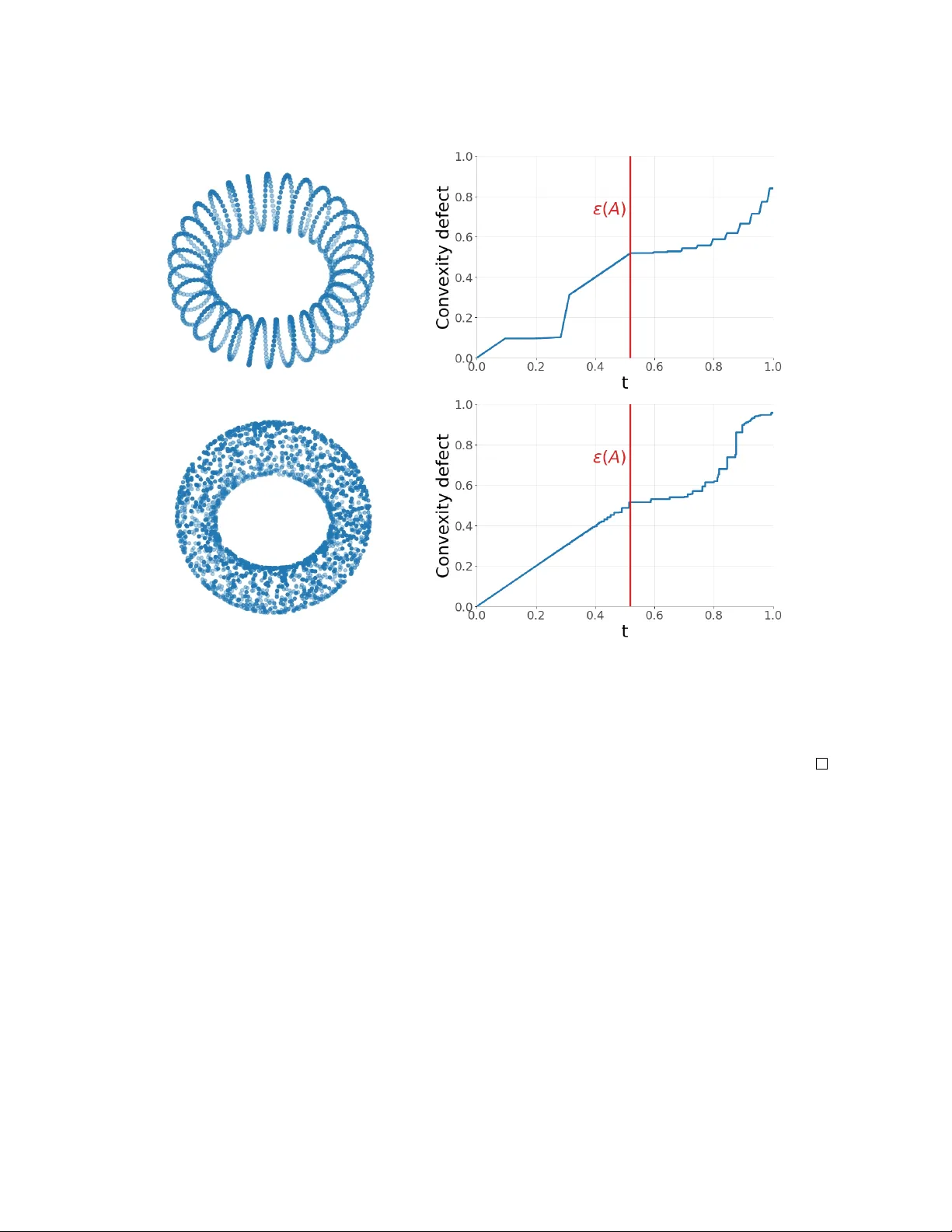
MINIMAX AD APTIVE ESTIMA TION IN MANIF OLD INFERENCE V inc ent Divol ∗ Abstract. W e fo cus on the problem of manifold estimation: giv en a set of observ ations sampled close to some unknown submanifold M , one w ants to reco ver information ab out the geometry of M . Minimax estimators which ha v e b een proposed so far all dep end crucially on the a priori kno wledge of parameters quan tifying the underlying distribution generating the sample (suc h as b ounds on its density), whereas those quantities will b e unknown in practice. Our con tribution to the matter is tw ofold. First, we in tro duce a one-parameter family of manifold estimators ( ˆ M t ) t ≥ 0 based on a lo calized v ersion of conv ex hulls, and show that for some c hoice of t , the corresp onding estimator is minimax on the class of models of C 2 manifolds in tro duced in [ GPPVW12 ]. Second, w e prop ose a completely data-driv en selection pro cedure for the parameter t , leading to a minimax adaptiv e manifold estimator on this class of mo dels. This selection pro cedure actually allows us to reco ver the Hausdorff distance b et ween the set of observ ations and M , and can therefore b e used as a scale parameter in other settings, such as tangen t space estimation. 1 Intro duction Manifold inference deals with the estimation of geometric quantities in a random setting. Giv en X n = { X 1 , . . . , X n } a set of i.i.d. observ ations from some la w µ on R D supp orted on (or con- cen trated around) a d -dimensional manifold M , one w an ts to pro duce an estimator ˆ θ that estimates accurately some quan tit y θ ( M ) related to the geometry of M suc h as its dimen- sion d [ HA05 , LJM09 , KR W19 ], its homology groups [ NSW08 , BRS + 12 ], its tangen t spaces [ AL19 , CC16 ], or M itself [ GPPVW12 , GPPIW12 , MMS16 , AL18 , AL19 , PS19 ]. Consider for instance the problem of estimating the manifold M with resp ect to the Hausdorff distance d H . The quality of an estimator ˆ M with resp ect to some la w µ , called its µ -risk, is given b y the a verage Hausdorff distance d H b et ween the estimator and M : R n ( ˆ M , µ ) : = E [ d H ( ˆ M , M )] , (1.1) where ˆ M = ˆ M ( X n ) and X n is a n -sample of law µ . In reality , the law µ generating the dataset is unknown, and it is more in teresting to control the µ -risk uniformly o v er a set Q of laws µ , ∗ Center for Data Scienc e and Cour ant Institute of Mathematic al Scienc e, New Y ork University firstname.lastname@nyu.edu 1 τ ( A ) A τ ( A ) A Figure 1: If the reac h of the curve M is large, then the curv e cannot be to o pinc hed (left) an d cannot presen t a tigh t b ottlenec k structure (right). that w e call a statistical mo del. The uniform risk of the estimator ˆ M on the class Q is giv en by , R n ( ˆ M , Q ) : = sup { R n ( ˆ M , µ ) : µ ∈ Q} . (1.2) while we sa y that an estimator is minimax if it attains (up to a m ultiplicativ e constant as n goes to ∞ ) the minimax risk R n ( Q ) : = inf { R n ( ˆ M , Q ) : ˆ M is an estimator } . (1.3) In geometric inference, several statistical mo dels w ere in tro duced, which tak e in to account differen t noise models and regularities of the manifold M . Let us men tion the family of mo dels Q d τ min ,f min ,f max in tro duced b y Geno vese et al. in [ GPPVW12 ], consisting of the la ws µ supp orted on a d -dimensional manifold M satisfying some additional prop erties. First, we assume that µ has a densit y f on M , low er b ounded by some constan t f min > 0 and upp er b ounded by another constant f max . This ensures that all the parts of the manifold M are approximately ev enly sampled: w e then say that the law is "almost-uniform" on M . The parameter τ min giv es a low er b ound on the reac h τ ( M ) of the manifold. The reac h is a central notion in geometric inference, defined as the largest radius r such that, if some p oint x is at distance less than r to M , then there exists a unique pro jection π M ( x ) of x on M . As suc h, it con trols b oth a lo cal regularit y of M (a b ound on its curv ature radius) and a global regularit y (namely the presence of a "b ottlenec k structure"), see also Figure 1 . On the statistical model Q d τ min ,f min ,f max , the minimax rate of con vergence satisfies c 0  ln n n  2 /d ≤ R n ( Q d τ min ,f min ,f max ) ≤ c 1  ln n n  2 /d , (1.4) for tw o positive constants c 0 , c 1 dep ending on τ min , f min , f max and d . The low er bound in this inequalit y was sho wn by Kim and Zhou [ KZ15 ], while the upp er b ound is obtained by exhibit- 2 ing an estimator ha ving a uniform risk of order (ln n/n ) 2 /d . Suc h an estimator (although not computable in practice) was first prop osed b y Geno v ese et al. in [ GPPVW12 ], while another estimator attaining this same minimax rate (computable in practice), and based on the T an- gen tial Delaunay Complex [ BG14 ], w as prop osed by Aamari and Levrard [ AL18 ]. Although b eing minimax and computable, the T angential Delauna y Complex dep ends on the tuning of sev eral parameters (for instance a radius quantifying the size of neigh b orhoo ds which are used to compute lo cal PCAs), while those parameters ha ve to b e calibrated in a precise manner with resp ect to the quantities τ min , f min and f max defining the model for the T angential Delaun y Complex to be minimax. Ho wev er, those quantities are a priori unkno wn. A first p ossibilit y is to estimate those quantities in turn: if pro cedures are known to estimate the reac h (although themselv es dep ending on the tuning of parameters [ AKC + 19 , BHHS21 ]), estimating f min and f max app ears to be delicate. The problem of the practical choice of the parameters defining the estimator is then raised. This question of the tuning of parameters defining an estimator is not restricted to the framew ork of manifold estimation, but is a classical problem in statistics. Let us cite for instance the question of the choice of the bandwidth for k ernel densit y estimation. Let X 1 , . . . , X n b e a n -sample of some law µ having a density f on R , and sup- p ose that we wan t to recov er the v alue f ( x 0 ) of the densit y at some fixed p oin t x 0 ∈ R . A standard metho d to ac hieve this goal is to consider the con volution of the empirical measure µ n = 1 n P n i =1 δ X i b y some k ernel K h , where K h = h − 1 K ( · /h ) and K satisfies R K = 1 . W e then obtain a function ˆ f = K h ∗ µ n . Assume that the density f is of regularity s , that is f ∈ C s ( R ) , the set of b s c -times differentiable functions, whose b s c th deriv ativ e is ( s − b s c ) -Hölder contin u- ous. Then, for a go od c hoice of k ernel K , it is optimal to c ho ose the bandwidth h opt of order c · n − 1 / (2 s +1) , where c dep ends on the C s -norm of f [ T sy08 , Chapter 1]. The asso ciated risk is then of order n − s/ (2 s +1) , which is the minimax rate of estimation on the class of densities of regularit y s . In practice, it is imp ossible to know exactly the v alue of s , so that w e must find another strategy to c ho ose the bandwidth h . A daptive methods consist in c ho osing a bandwidth ˆ h in a data-dep enden t wa y , suc h that the estimator ˆ f ˆ h has a µ -risk almost as go od as the opti- mal estimator ˆ f h opt under weak hypotheses on µ . One of suc h metho ds, the PCO metho d (for P enalized Comparison to Overfitting) introduced by Lacour, Massart and Rivoirard [ LMR17 ] consists in comparing eac h estimator ˆ f h to some degenerate estimator ˆ f h min for some very small bandwidth h min . The selected bandwidth ˆ h is c hosen among a family H of bandwidths (all larger than h min ), b y minimizing a criterion dep ending on the distance k ˆ f h − ˆ f h min k L 2 ( R ) , while p enalizing small v alues of h . Lacour, Massart and Riv oirard then show an oracle inequalit y for their estimator, that is an inequalit y of the form E k ˆ f ˆ h − f k 2 L 2 ( R ) ≤ C min { E k ˆ f h − f k 2 L 2 ( R ) : h ∈ H} + C ( n, |H| ) (1.5) where C ( n, |H| ) is a remainder term negligible in fron t of the optimal risk. Thus, we obtain that ˆ f ˆ h has a risk almost as go od as the b est estimator ˆ f h opt , while w e never had to estimate the parameters defining the statistical mo del (that is the regularity s of the densit y and the C s -norm of f ). 3 Figure 2: The t -conv ex hull Conv( t, A ) (in green) of a curv e A (in black). Our main goal is to adapt the PCO metho d to the manifold inference setting. A first step consists in creating a family of estimators ( ˆ M t ) t ≥ 0 similar to kernel densit y estimators, but in the context of manifold estimation. This is made p ossible with t -con vex hulls. F or t ≥ 0 , the t -con vex hull Conv( t, A ) of a set A is an interpolation b et ween the set A ( t = 0 ) and its con vex h ull Con v( A ) ( t = ∞ ). It is defined as Con v( t, A ) : = [ σ ⊆ A r ( σ ) ≤ t Con v( σ ) , (1.6) where r ( σ ) is the radius of the set σ , that is the radius of the smallest enclosing ball of σ . See Figure 2 for an example. W e prov e in Section 3 that for A ⊆ M , the Hausdorff distance b et ween Conv( t, A ) and M can b e efficiently controlled for v alues of t a little larger than the appro ximation rate ε ( A ) : = sup { d ( x, A ) : x ∈ M } of A . More precisely , for suc h v alues of t , Lemma 3.3 states that d H (Con v( t, A ) , M ) ≤ t 2 /τ ( M ) . Using this control on the t -con vex h ull enables us to sho w that the t -conv ex hull of the sample X n is a minimax estimator on the mo del Q d τ min ,f min ,f max for a certain c hoice of t . Theorem 1.1. L et α d b e the volume of the d -dimensional unit b al l. F or the choic e of sc ale t n = 7 4 (3 ln n/ ( α d f min n )) 1 /d , we have (for n lar ge enough) R n (Con v( t n , X n ) , Q d τ min ,f min ,f max ) ≤ c 0 τ min ( α d f min ) 2 /d  ln n n  2 /d (1.7) for some absolute c onstant c 0 . In other wor ds, Conv( t n , X n ) is a minimax estimator of M on Q d τ min ,f min ,f max . T o create an adaptive estimator, the next step is to build a selection pro cedure for the parameter t . An analog of the degenerate estimator ˆ f h min is given b y the c hoice t = 0 , with 4 Con v(0 , X n ) = X n . The PCO metho d therefore suggests comparing the estimators Conv( t, X n ) with X n , that is to study the function t 7→ h ( t, X n ) : = d H (Con v( t, X n ) , X n ) . The function h ( · , X n ) w as actually already introduced under the name of "conv exity defect function of the set X n " in a pap er by A ttali, Lieutier and Salinas [ ALS13 ], where it was used to study the homotop y types of Rips complexes. The conv exity defect function is nonnegative, nondecreasing, and satisfies 0 ≤ h ( t, A ) ≤ t for an y set A . F or A = X n , this function is piecewise constan t, while it ma y only c hange v alues at t ∈ Rad( X n ) : = { r ( σ ) : σ ⊆ X n } . W e show that the con vexit y defect function h ( t, X n ) of X n at scale t exhibits different b eha viors in tw o differen t regimes: for t ≤ ε ( X n ) it has a globally linear b eha vior (that is it sta ys close to its maximal v alue t ), whereas roughly after ε ( X n ) , it is almost constant. The con vexit y defect function can b e computed using only the dataset, so that we may in practice observ e those tw o regimes. In practice, w e fix a v alue 0 < λ < 1 , and let t λ ( X n ) : = inf { t ∈ Rad( X n ) : h ( t, X n ) ≤ λt } . (1.8) Our main result states that t λ ( X n ) is a little larger than ε ( X n ) with high probabilit y , so that we may control the risk of ˆ M = Conv( t λ ( X n ) , X n ) , without ha ving to know d , f min , f max or the reac h τ ( M ) , leading to an adaptiv e estimator in a sense made precise in Theorem 6.2 . The estimator ˆ M is to our kno wledge the first minimax adaptiv e manifold estimator. Our pro cedure allo ws us to actually estimate (up to a multiplicativ e constan t arbitrarily close to 1 ) the appro ximation rate ε ( X n ) , while scale parameters in computational geometry t ypically hav e to b e prop erly tuned with resp ect to this quantit y . The parameter t λ ( X n ) can therefore b e used as a h yp erparameter in different settings. T o illustrate this general idea, w e show ho w to create a data-driv en minimax estimator of the tangen t spaces of a manifold (see Corollary 6.5 ). Related w o rk "Lo calized" v ersions of con vex h ulls such as the t -con vex h ulls hav e already b een introduced in the supp ort estimation literature. F or instance, slightly mo dified versions of the t-conv ex h ull ha ve been used as estimators in [ AB16 ] under the assumption that the supp ort has a smo oth b oundary and in [ R C07 ] under reach constraints on the supp ort, with differen t rates obtained in those mo dels. Selection pro cedures w ere not designed in those t w o pap ers, and whether our selection procedure leads to an adaptive estimator in those framew orks is an interesting question. The statistical mo dels we study in this article were introduced in [ GPPVW12 ] and [ AL18 ], in which manifold estimators w ere also prop osed. If the estimator in [ GPPVW12 ] is of purely theoretical in terest, the estimator prop osed by Aamari and Levrard in [ AL18 ], based on the T angen tial Delauna y complex, is computable with O ( nD 2 O ( d 2 ) ) op erations. F urthermore, it is a simplicial complex which is kno wn to b e ambien t isotopic to the underlying manifold M with high probabilit y . It ho w ever requires the tuning of sev eral h yp erparameters in order to b e minimax, which ma y make its use delicate in practice. In con trast, the t -con v ex hull estimator 5 with parameter t λ ( X n ) is completely data-driv en, computable in polynomial time (see Section 7 ), while k eeping the minimax prop ert y . How ev er, unlike in the case of the T angential Delaunay complex, w e ha ve no guarantees on the homotopy type of the corresp onding estimator. 2 Background on submanifold with p ositive reach Let us first introduce some notation. The Euclidean norm in R D is denoted b y | · | and h· , ·i stands for the dot product. If A ⊆ R D and x ∈ R D , then d ( x, A ) := inf {| x − y | : y ∈ A } is the distance to a set A while diam( A ) := sup {| x − y | : x, y ∈ A } is its diameter. Given r ≥ 0 , B ( x, r ) is the op en ball of radius r centered at x and w e write B A ( x, r ) for B ( x, r ) ∩ A . W e let M d b e the set of C 2 compact connected d -dimensional submanifolds of R D without b oundary . If M ∈ M d and x ∈ M , then T x M is the tangent space of M at x . It is identified with a d -dimensional subspace of R D , and we write π x for the orthogonal pro jection on T x M , while π ⊥ x = id − π x is the pro jection on the normal space T x M ⊥ . The asymmetric Hausdorff distance b etw een sets A, B ⊆ R D is defined as d H ( A | B ) := sup { d ( x, B ) : x ∈ A } , while the Hausdorff distance is defined as d H ( A, B ) = max { d H ( A | B ) , d H ( B | A ) } . F or A ⊆ M , we denote by ε ( A ) := d H ( A, M ) the appro ximation rate of A . The regularity of a submanifold M ∈ M d is measured by its reac h τ ( M ) . This is the largest num b er r suc h that if d ( x, M ) < r for x ∈ R D , then there exists a unique p oin t of M , denoted b y π M ( x ) , which is at distance d ( x, M ) from x . Thus, the pro jection π M on the manifold M is well-defined on the r -tubular neigb orho od M r := { x ∈ M : d ( x, M ) ≤ r } for r < τ ( M ) . The notion of reac h was in tro duced for general sets by F ederer in [ F ed59 ], where it is also pro v en that C 2 compact submanifolds without b oundary hav e p ositiv e reac h (see [ F ed59 , p.432]). Differen t geometric quan tities of interest can b e b ounded in term of the reac h. F or instance, the v olume V ol( M ) of M satisfies V ol( M ) ≥ ω d τ ( M ) d (2.1) where ω d is the volume of a d -dimensional sphere (with equalit y obtained only for a sphere of radius τ ( M ) ), see [ Alm86 ]. The reac h also controls how p oin ts on M deviate from their pro jections on some tangent s pace. Lemma 2.1 (Theorem 4.18 in [ F ed59 ]) . F or x, y ∈ M ,    π ⊥ x ( y − x )    ≤ | y − x | 2 2 τ ( M ) . The follo wing lemma asserts that the pro jection from a manifold to its tangen t space is w ell-b eha ved. Lemma 2.2. L et x ∈ M . 1. L et y ∈ R D with d ( y , M ) < τ ( M ) . Then, π M ( y ) = x if and only if y − x ∈ T x M ⊥ . 6 2. L et y 1 , y 2 ∈ R D b e two p oints at distanc e less than γ < τ ( M ) fr om M . Then, | π M ( y 1 ) − π M ( y 2 ) | ≤ τ ( M ) τ ( M ) − γ | y 1 − y 2 | . 3. F or r < τ ( M ) / 3 , the map ˜ π x : y 7→ π x ( y − x ) is a diffe omorphism fr om B M ( x, r ) to its image, and, if r ≤ τ ( M ) / 2 , we have B T x M (0 , 7 r / 8) ⊆ ˜ π x ( B M ( x, r )) . In p articular, if y ∈ B M ( x, 7 τ ( M ) / 24) , then 7 8 | y − x | ≤ | π x ( y − x ) | ≤ | y − x | . (2.2) Pr o of. • F or 1 and 2, see [ F ed59 , Theorem 4.8]. • W e first show that ˜ π x is injectiv e on B M ( x, τ ( M ) / 3) . Assume that ˜ π x ( y ) = ˜ π x ( y 0 ) for some y 6 = y 0 ∈ M . Consider without loss of generalit y that | x − y | ≥ | x − y 0 | . The goal is to sho w that | x − y | ≥ τ ( M ) / 3 . If | x − y | > τ ( M ) / 2 , the conclusion obviously holds, so we ma y assume that | x − y | ≤ τ ( M ) / 2 . Define the angle b et ween T x M and T y M as k π x − π y k op (where k · k op denotes the operator norm). Lemma 3 . 4 in [ BSW09 ] states that if | x − y | ≤ τ ( M ) / 2 , then ∠ ( T x M , T y M ) ≤ 2 | x − y | τ ( M ) . Also, by definition, ∠ ( T x M , T y M ) ≥ | ( π x − π y ) ( y − y 0 ) | | y − y 0 | = | π y ( y − y 0 ) | | y − y 0 | ≥ | y − y 0 | −    π ⊥ y ( y − y 0 )    | y − y 0 | ≥ 1 − | y − y 0 | 2 τ ( M ) b y Lemma 2.1 ≥ 1 − | x − y | τ ( M ) b y the triangle inequalit y . Therefore, we hav e 3 | x − y | /τ ( M ) ≥ 1 , i.e. | x − y | ≥ τ ( M ) / 3 and ˜ π x is injective on B M ( x, τ ( M ) / 3) . T o conclude that ˜ π x is a diffeomorphism, it suffices to show that its differential is alw ays inv ertible. As ˜ π x is an affine application, the differential d ˜ π x ( y ) is equal to π x . Therefore, the Jacobian of the function ˜ π x : M → T x M at y is given b y the determinant of the pro jection π x restricted to T y M . In particular, it is larger than the smallest singular v alue of π x ◦ π y to the p o wer d , which is larger than (1 − ∠ ( T x M , T y M )) d ≥  1 − 2 | x − y | τ ( M )  d ≥  1 3  d thanks to [ BSW09 , Lemma 3.4] and using that | x − y | ≤ τ ( M ) / 3 . In particular, the Jacobian is p ositiv e, and ˜ π x is a diffeormorphism from B M ( x, τ ( M ) / 3) to its image. The second statemen t is stated in [ AL19 , Lemma A.2]. 7 The second inequality of the last statement follows from the pro jection b eing 1-Lipschitz con tinuous. F or the first one, let y ∈ B M ( x, 7 τ ( M ) / 24) , and let u = π x ( y − x ) . The p oin t u is in B T x M (0 , h ) for h > | u | . W e ha ve B T x M (0 , h ) ⊆ ˜ π x ( B M ( x, 8 h/ 7)) ⊆ ˜ π x ( B M ( x, τ ( M ) / 3)) . As ˜ π x is injectiv e on B M ( x, τ ( M ) / 3) , this means that w e necessarily ha v e y ∈ B M ( x, 8 h/ 7) . Therefore, | x − y | < 8 h/ 7 , and the conclusion holds b y letting h go es to | u | . It will also b e necessary to hav e precise b ounds on the v olume of balls on M . As exp ected, the v olume of a small ball is asymptotically equiv alent to the v olu me of an Euclidean ball. Let α d b e the volume of the d -dimensional unit ball. Lemma 2.3. L et r ≤ τ ( M ) / 4 and x ∈ M . Then,  47 48  d ≤ 1 − r 2 3 τ ( M ) 2 ! d ≤ V ol ( B M ( x, r )) α d r d ≤ 1 + 4 r 2 3 τ ( M ) 2 ! d ≤  13 12  d . (2.3) Pr o of. The proof of Prop osition 8.7 in [ AL18 ] implies that, if ˜ B M ( x, r ) is the geo desic ball cen tered at x of radius r , then 1 − r 2 3 τ ( M ) 2 ! d ≤ V ol  ˜ B M ( x, r )  α d r d ≤ 1 + r 2 τ ( M ) 2 ! d . As ˜ B M ( x, r ) ⊆ B M ( x, r ) , we hav e in particular V ol( B M ( x,r )) α d r d ≥  1 − r 2 3 τ ( M ) 2  d . F urther- more, by [ A CLG19 , Lemma 3.12] and [ NSW08 , Prop osition 6.3], if | x − y | ≤ τ ( M ) / 4 , then the geo desic distance b et ween x and y is smaller than | x − y | 1 + π 2 50 τ ( M ) 2 | x − y | 2 ! ≤ 1 . 05 | x − y | . This implies that B M ( x, r ) ⊆ ˜ B M  x, r  1 + π 2 r 2 50 τ ( M ) 2  . Therefore, V ol ( B M ( x, r )) α d r d ≤ 1 + π 2 r 2 50 τ ( M ) 2 ! 1 + (1 . 05 r ) 2 τ ( M ) 2 !! d ≤ 1 + π 2 50 + (1 . 05) 2 + π 2 (1 . 05) 2 r 2 50 τ ( M ) 2 ! r 2 τ ( M ) 2 ! ≤ 1 + 4 r 2 3 τ ( M ) 2 ! d , where w e used at the last line that r ≤ τ ( M ) / 4 . 8 3 App ro ximation of manifolds with t -convex hulls Let A ⊆ M b e a finite set. W e inv estigate in this section ho w the t -conv ex h ull of A approx- imates M for differen t v alues of t , first in a deterministic setting, then in a random setting. The quan tit y of interest d H (Con v( t, A ) , M ) is by definition the maximum of the t wo quan tities d H (Con v( t, A ) | M ) and d H ( M | Con v( t, A )) . The first quantit y d H (Con v( t, A ) | M ) is given b y the maxim um of the distances d H (Con v( σ ) | M ) ov er the simplexes σ ⊆ A satisfying r ( σ ) ≤ t. A naiv e attempt to b ound this quantit y leads to a control of order t . Lemma 3.1. L et σ ⊆ R D b e a close d set. Then, d H (Con v( σ ) | σ ) ≤ r ( σ ) . Pr o of. Let y ∈ Con v( σ ) and let z b e the cen ter of the smallest enclosing ball of σ . The half-space n x ∈ R D : | x − z | 2 − r ( σ ) 2 ≤ | x − y | 2 − d ( y , σ ) 2 o con tains σ . It thus con tains Conv( σ ) , and in particular y . Therefore, d ( y , σ ) 2 ≤ r ( σ ) 2 − | y − z | 2 ≤ r ( σ ) 2 , concluding the proof. As σ ⊆ M , we ha ve in particular that d H (Con v( t, A ) | M ) ≤ t . W e can actually obtain a m uch b etter b ound by exploiting that σ lies on M , which lo oks locally lik e a flat space. Consider for instance the case where σ = { x 0 , x 1 } is made of t wo points. Then, the line ( x 0 , x 1 ) should b e appro ximately parallel to the tangent space T x 0 M , with the distance from x 1 to T x 0 M b eing of order | x 0 − x 1 | 2 . As a consequence, the distance from an y p oin t of the segment [ x 0 , x 1 ] to M is also of order | x 0 − x 1 | 2 . More generally , w e hav e the following result. Lemma 3.2. L et σ ⊆ M with r ( σ ) < τ ( M ) and let y ∈ Con v( σ ) . Then, d ( y , M ) ≤ τ ( M ) 1 − s 1 − r ( σ ) 2 τ ( M ) 2 ! ≤ r ( σ ) 2 2 τ ( M ) 1 + r ( σ ) 2 τ ( M ) 2 ! . (3.1) In p articular, for any t ≥ 0 and A ⊆ M , d H (Con v( t, A ) | M ) ≤ t 2 2 τ ( M ) " 1 + t 2 τ ( M ) 2 ! ∧ 2 # ≤ t 2 τ ( M ) . (3.2) Pr o of. Lemma 12 in [ ALS13 ] states that if σ ⊆ M satisfies r ( σ ) < τ ( M ) and y ∈ Con v ( σ ) , then, d ( y , M ) ≤ τ ( M ) 1 − s 1 − r ( σ ) 2 τ ( M ) 2 ! . As √ 1 − u ≥ 1 − u/ 2 − u 2 / 2 for u ∈ [0 , 1] , one obtains the conclusion. 9 t ≥ t ∗ ( A ) t < t ∗ ( A ) Figure 3: The t -conv ex hull of the finite set A (red crosses) is display ed (in green) for tw o v alues of t . The black curv e represen ts the (one dimensional) manifold M . On the first display , the v alue of t is smaller than t ∗ ( A ) , as there are regions of the manifold (circled in blue) whic h are not attained by the pro jection π M restricted to the t -con vex h ull. The v alue of t is larger than t ∗ ( A ) on the second displa y . The other asymmetric distance d H ( M | Con v( t, A )) is apparently more delicate to handle. It can actually b e controlled efficiently if the parameter t is large enough. Indeed, assume that t is large enough so that ev ery p oint x of M is the projection of some p oin t y of Conv( t, A ) . Then w e ha ve d ( x, Con v( t, A )) ≤ | x − y | = | π M ( y ) − y | = d ( y , M ) ≤ d H (Con v( t, A ) | M ) ≤ t 2 τ ( M ) . (3.3) This suggests defining the parameter t ∗ ( A ) := inf { t < τ ( M ) : π M (Con v( t, A )) = M } . (3.4) Lemma 3.2 and ( 3.3 ) imply directly the following lemma. Lemma 3.3. L et A ⊆ M and t > t ∗ ( A ) . Then, d H (Con v( t, A ) , M ) ≤ t 2 τ ( M ) . (3.5) A crucial result in the analysis of the t -con vex h ull estimator is given by the next prop o- sition, that indicates that the quan tity t ∗ ( A ) is almost equal to the approximation rate ε ( A ) . 10 Prop osition 3.4. L et A ⊆ M b e a finite set. Then, ε ( A ) ≤ t ∗ ( A )  1 + t ∗ ( A ) τ ( M )  . F urthermor e, if ε ( A ) < τ ( M ) / 8 , then, t ∗ ( A ) ≤ ε ( A )  1 + 6 ε ( A ) τ ( M )  The pro of of Prop osition 3.4 relies on cons idering Delaunay triangulations. Given d + 1 p oin ts σ in R d that do not lie on a hyperplane, there exists a unique ball that contains the p oin ts on its b oundary . It is called the circumball of σ , and its radius is called the circumradius circ( σ ) of σ . Given a finite set A ⊆ R d that does not lie on a h yp erplane, there exists a triangulation of A , called the Delaunay triangulation, such that for eac h simplex σ in the triangulation, the circum ball of σ con tains no p oin t of A in its interior. Note that there may exist sev eral Delaunay triangulations of a set A , should the set A not b e in general position. With a slight abuse, w e will still refer to "the" Delauna y triangulation of A , b y simply c ho osing a Delaunay triangulation among the p ossible ones should sev eral exist. If the set A lies on a low er dimensional subspace, we consider the Delaunay triangulation of A in the affine v ector space spanned by A . Therefore, for ev ery set A , the Delaunay triangulation is well defined (for instance, the Delauna y triangulation of three p oin ts aligned in the plane is the 1-dimensional triangulation obtained by joining the middle p oin t with the tw o others). Pr o of. Let x ∈ M b e such that d ( x, A ) = ε ( A ) . By definition, there exists a simplex σ ⊆ A of radius smaller than t ∗ ( A ) with x = π M ( y ) for some p oin t y ∈ Con v( σ ) . W e hav e, using Lemma 3.1 and Lemma 3.2 , ε ( A ) = d ( x, A ) ≤ | x − y | + d ( y , A ) ≤ t ∗ ( A ) 2 τ ( M ) + t ∗ ( A ) pro ving the first inequalit y . T o prov e the other inequality , without loss of generalit y , we assume that 0 ∈ M and w e sho w that 0 ∈ π M (Con v( t, A )) for t = ε ( A )(1 + 6 ε ( A ) /τ ( M )) . Let ˜ A = π 0 ( A ∩ B (0 , R )) for R = ε ( A ) (2 + c 0 ε ( A ) /τ ( M )) and c 0 = 32 / 49 . Note that the condition ε ( A ) ≤ τ ( M ) / 8 implies that R < 7 τ ( M ) / 24 . W e first state tw o lemmas. Lemma 3.5. A ssume that ε ( A ) ≤ 7 τ ( M ) / 24 . L et ˜ x ∈ T 0 M with | ˜ x | ≤ ε ( A ) . Then d ( ˜ x, ˜ A ) ≤ ε ( A ) . Pr o of. By con tinuit y , it suffices to pro ve the claim for | ˜ x | < ε ( A ) . In this case, according to Lemma 2.2 , if ε ( A ) ≤ 7 τ ( M ) / 24 , then there exists x ∈ B M (0 , 8 ε ( A ) / 7) with π 0 ( x ) = ˜ x . F urthermore, by Lemma 2.1 , | x | ≤ | ˜ x | + | x − ˜ x | ≤ ε ( A ) + | x | 2 2 τ ( M ) ≤ ε ( A )  1 + 32 ε ( A ) 49 τ ( M )  . 11 W e hav e d ( x, A ) = | x − a | for some p oin t a ∈ A , and | a | ≤ | x − a | + | x | ≤ ε ( A ) (2 + c 0 ε ( A ) /τ ( M )) . As π 0 ( a ) ∈ ˜ A , w e ha ve d ( ˜ x, ˜ A ) ≤ | ˜ x − π 0 ( a ) | ≤ | x − a | = d ( x, A ) ≤ ε ( A ) . Lemma 3.6. L et V ⊆ R d b e a finite set and t > 0 . If d H ( B (0 , t ) | V ) ≤ t , then 0 ∈ Conv( V ) . Pr o of. W e pro ve the contrapositive. If 0 / ∈ Conv( V ) , then there exists an op en half-space which con tains V . Let x b e the unit v ector orthogonal to this half-space. Then, d ( tx, V ) > t . Apply Lemma 3.6 to V = ˜ A and t = ε ( A ) . F or ˜ x ∈ B T 0 M (0 , ε ( A )) , we hav e d ( ˜ x, ˜ A ) ≤ ε ( A ) according to Lemma 3.5 . Therefore, we ha v e 0 ∈ Con v( ˜ A ) . Consider the Delaunay triangulation of ˜ A . The p oin t 0 b elongs to the conv ex hull of some simplex ˜ σ of the triangulation, with circumradius circ( ˜ σ ) and center of the circumball ˜ q . The simplex ˜ σ corresp onds to some simplex σ in A , and the p oin t 0 is equal to π 0 ( y ) for some p oin t y ∈ Conv( σ ) . By Lemma 2.2 , we actually hav e π M ( y ) = 0 , and to conclude, it suffices to sho w that r ( σ ) ≤ ε ( A )  1 + 6 ε ( A ) τ ( M )  . T o do so, w e use the next lemma (recall that σ ⊆ B M (0 , R ) with R < 7 τ ( M ) / 24) . Lemma 3.7. L et σ ⊆ B M (0 , 7 τ ( M ) / 24) and ˜ σ = ˜ π 0 ( σ ) . A ssume that 0 ∈ Con v( ˜ σ ) . Then, r ( ˜ σ ) ≤ r ( σ ) ≤ r ( ˜ σ )  1 + 6 r ( ˜ σ ) τ ( M )  . (3.6) Pr o of. As the pro jection is 1-Lipschitz, it is clear that r ( ˜ σ ) ≤ r ( σ ) . Let us pro v e the other inequalit y . Let σ = { y 0 , . . . , y k } , ˜ σ = { ˜ y 0 , . . . , ˜ y k } and fix 0 ≤ i ≤ k . As y i ∈ B M (0 , 7 τ ( M ) / 24) , w e ha ve by ( 2.2 ) | y i | ≤ 8 7 | ˜ y i | ≤ 16 7 r ( ˜ σ ) . (3.7) where we used that | ˜ y i | ≤ 2 r ( ˜ σ ) as 0 ∈ Con v( ˜ σ ) . Let ˜ z b e the cen ter of the minim um enclosing ball of ˜ σ . W rite ˜ z = P k j =0 λ j ˜ y j as a con vex combination of the ˜ y j s and let z = P k j =0 λ j y j ∈ Con v( σ ) . Then, we ha ve | z − y i | ≤ | z − ˜ z | + | ˜ z − ˜ y i | + | ˜ y i − y i | ≤ k X j =0 λ j | y j − ˜ y j | + r ( ˜ σ ) + | y i | 2 2 τ ( M ) using Lemma 2.1 ≤ k X j =0 λ j | y j | 2 2 τ ( M ) + r ( ˜ σ ) + 128 49 r ( ˜ σ ) 2 τ ( M ) using Lemma 2.1 and ( 3.7 ) ≤ r ( ˜ σ ) + 256 49 r ( ˜ σ ) 2 τ ( M ) ≤ r ( ˜ σ ) + 6 r ( ˜ σ ) 2 τ ( M ) using ( 3.7 ). 12 0 ˜ w ε ( A ) ˜ q Figure 4: If | ˜ q | > ε ( A ) , then the ball B T 0 M ( ˜ q , | ˜ q | ) con tains a ball of radius ε ( A ) cen tered at a p oin t (here denoted by ˜ w ) at distance less than ε ( A ) from 0. W e obtain the conclusion as σ is included in the ball of radius max i | z − y i | and center z . Using the previous lemma, w e are left with sho wing that r ( ˜ σ ) ≤ ε ( A ) . W e will actually sho w the stronger inequalit y circ( ˜ σ ) ≤ ε ( A ) (the radius of a set is alwa ys smaller than its circumradius). As 0 is in the circumball (that is cen tered at ˜ q ), the ball cen tered at ˜ q of radius | ˜ q | does not in tersect ˜ A . This enforces | ˜ q | ≤ ε ( A ) : otherwise, there would exist a ball not intersecting ˜ A , of radius ε ( A ) , and whose center is at distance less than ε ( A ) from 0, a con tradiction with Lemma 3.5 (see Figure 4 ). As | ˜ q | ≤ ε ( A ) , we obtain, once again according to Lemma 3.5 , that circ( ˜ σ ) = d ( ˜ q , ˜ A ) ≤ ε ( A ) concluding the pro of. Remark 3.8. In the c ase wher e the dimension d is known, one c an c onsider a variant of the t -c onvex hul l, Con v d ( t, A ) , wher e one r estricts the union to b e over simplic es of dimension less than d . The set Con v d ( t, A ) is simpler to c ompute as it c ontains less simplic es (se e Se ction 7 ). F urthermor e, if t ∗ d ( A ) := inf { t : π M (Con v d ( t, A )) = M } , then b oth L emma 3.3 and Pr op osition 3.4 hold with t ∗ d ( A ) and Conv d ( t, A ) inste ad of t ∗ ( A ) and Conv( t, A ) . Inde e d, only simplic es of dimension less than d (c orr esp onding to simplic es of a Delaunay triangulation on a tangent sp ac e) wer e c onsider e d in the pr evious pr o of. W e ha v e now shown that the quality of the t -con vex hull on A can b e con trolled for t ≥ ε ( A )(1 + 6 ε ( A ) /τ ( M )) (that is slightly larger than the appro ximation rate ε ( A )) . In a random setting, the appro ximation rate is known to b e of order (ln n/n ) 1 /d : this is enough to sho w that the t -conv ex h ull is a minimax estimator. Recall the definition of the statistical mo del Q d τ min ,f min ,f max from the introduction: it consists of laws µ supp orted on some manifold M ∈ M d with τ ( M ) ≥ τ min , ha ving a density f low er bounded b y f min and upp er bounded b y f max . The 13 minimax result will actually hold on the larger mo del Q d τ min ,f min := S f max Q d τ min ,f min ,f max (that is without imp osing any upper b ound on f ). Let µ ∈ Q d τ min ,f min and let X n b e a n -sample from la w µ . W e consider the estimator Con v( t, X n ) . Note first that Conv( t, X n ) is indeed an estimator, that is the application ( x 1 , . . . , x n ) ∈  R D  n 7→ Conv( t, { x 1 , . . . , x n } ) is measurable (with resp ect to the Borel σ -field asso ciated with the metric d H on the set K  R D  of all nonempty compact subsets of R D ). Indeed, for E a measurable subset of K  R D  and A, B ∈ K  R D  , introduce the notation G E ( A, B ) = A if A ∈ E and B otherwise. This function is measurable, and Con v ( t, { x 1 , . . . , x n } ) can be written as [ I ⊆{ 1 ,...,n } G E  Con v( { x i } i ∈ I  , { x i } i ∈ I ) where E is the subset of K  R D  giv en by n K ∈ K  R D  : r ( K ) ≤ t o , whic h is closed [ ALS13 , Lemma 16]. As the functions ∪ and Con v are measurable, the measurability follows [ Aam17 , Prop osition I I I.7]. F or a fixed t > 0 , w e obtain the follo wing con trol of E [ d H (Con v( t, X n ) , M )] . E [ d H (Con v( t, X n ) , M )] = E [ d H (Con v( t, X n ) , M ) 1 { t ≥ t ∗ ( X n ) } ] + E [ d H (Con v( t, X n ) , M ) 1 { t < t ∗ ( X n ) } ] ≤ t 2 τ ( M ) + diam ( M ) P ( t ∗ ( X n ) > t ) By Prop osition 3.4 , if ε ( X n ) < τ ( M ) / 8 , then t ∗ ( X n ) ≤ ε ( X n )  1 + 6 ε ( X n ) τ ( M )  ≤ 7 4 ε ( X n ) . Therefore, if t is small enough, P ( t ∗ ( X n ) > t ) ≤ P ( ε ( X n ) > τ ( M ) / 8) + P ( ε ( X n ) > 4 t/ 7) ≤ 2 P ( ε ( X n ) > 4 t/ 7) . W e obtain E [ d H (Con v( t, X n ) , M )] ≤ t 2 τ ( M ) + 2 diam ( M ) P ( ε ( X n ) > 4 t/ 7) (3.8) 14 Hence, to con trol the risk, it suffices to bound the tail of ε ( X n ) . Prop osition 3.9. L et µ ∈ Q d τ min ,f min and let X n = { X 1 , . . . , X n } b e a n -sample of law µ. If r ≤ τ min / 4 , then, for any η ∈ (0 , 1) P ( ε ( X n ) > r ) ≤ c d,η f min r d exp   − nα d f min 1 − r 2 3 τ 2 min ! d η r d   , (3.9) wher e c d,η dep ends on d and η . F urthermor e, for any a > 0 , for n lar ge enough (with r esp e ct to d , f min , τ min and a ), with pr ob ability 1 − c (ln n ) d − 1 n 1 − a (wher e c dep ends also on those p ar ameters), we have ε ( X n ) ≤  a ln n α d f min n  1 /d . (3.10) Pr o of. A measure ν is said to b e ( a, b ) -standard at scale r 0 if ν ( B ( x, r )) ≥ ar b for all r ≤ r 0 and x in the supp ort of ν . Let µ ∈ Q d τ min ,f min with supp ort M . Lemma 2.3 indicates that the measure µ is ( a, b ) -standard at scale r 0 for an y r 0 ≤ τ ( M ) / 4 , with a = f min α d  1 − r 2 0 3 τ ( M ) 2  d and b = d . It is stated in the pro of [ Aam17 , Prop osition II I.14] that for such a measure, and for an y δ ≤ 2 r 0 with 0 < r − δ ≤ r 0 , w e ha ve P ( ε ( X n ) > r ) ≤ 2 b aδ b exp  − na ( r − δ ) b  . Letting r = r 0 and δ =  1 − η 1 /d  r for some η ∈ (0 , 1) , we obtain that P ( ε ( X n ) > r ) ≤  2 /  1 − η 1 /d  d f min α d  1 − r 2 3 τ ( M ) 2  d r d exp   − nf min α d 1 − r 2 3 τ ( M ) 2 ! d η r d   ≤ c d 0 f min α d r d exp   − nf min α d 1 − r 2 3 τ ( M ) 2 ! d η r d   (3.11) for c 0 = 96 /  47  1 − η 1 /d  , where w e used at the last line that r ≤ τ ( M ) / 4 . T o prov e the second statement, w e let r =  a ln n α d f min n  1 /d . Then, we hav e nα d f min r d = a ln n . Letting η = 1 − 1 / ln n , we obtain that 15 nf min α d 1 − r 2 3 τ ( M ) 2 ! d η r d = ( a ln n )  1 − 1 ln n  1 − c  ln n n  2 /d ! ≥ ( a ln n ) − C a . In particular, w e obtain that the upper b ound in ( 3.11 ) is of order (ln n ) d − 1 n 1 − a . Cho ose t such that 4 t/ 7 =  3 ln n α d f min n n  1 /d . Then, according to Prop osition 3.9 , we hav e P ( ε ( X n ) > 32 t/ 7) ≤ c (ln n ) d − 1 n − 2 . As diam( M ) is also b ounded b y a constant dep ending on τ min , f min and d (see [ Aam17 , Lemma I II.24]), w e obtain Theorem 1.1 from ( 3.8 ) (without ev en the need of assuming that the density f is upp er b ounded). 4 Selection p ro cedure for the t -convex hulls Assuming that w e hav e observed a n -sample X n ha ving a distribution µ ∈ P d τ min ,f min , w e were able in the previous section to build a minimax estimator of the underlying manifold M . The tuning of this estimator requires the kno wledge of d and f min : if the dimension d can b e effi- cien tly estimated, this is not the case for f min , which will lik ely not b e accessible in practice. An idea to o vercome this issue is to design a selection pro cedure for the family of estimators (Con v( t, X n )) t ≥ 0 . As the loss of the estimator Con v ( t, X n ) is controlled efficiently for t ≥ t ∗ ( X n ) a go o d idea is to select a scale t larger than t ∗ ( X n ) . W e how ever do not hav e access to this quan tity based on the observ ations X n , as the manifold M is unkno wn. T o select a scale close to t ∗ ( X n ) , we monitor ho w the estimators Con v( t, X n ) deviate from X n as t increases. Namely , w e use the con vexit y defect function in tro duced in [ ALS13 ]. Definition 4.1. L et A ⊆ R D and t > 0 . The c onvexity defe ct function at sc ale t of A is define d as h ( t, A ) := d H (Con v( t, A ) , A ) . (4.1) As its name indicates, the conv exit y defect function measures the (lack of ) con vexit y of a set A at a giv en scale t . The next prop osition states preliminary results on the conv exity defect function. Prop osition 4.2. L et A ⊆ R D b e a close d set and t ≥ 0 . 1. W e have 0 ≤ h ( t, A ) ≤ t . 2. The set A is c onvex if and only if h ( · , A ) ≡ 0 . 3. If M ∈ M d , then h ( t, M ) ≤ t 2 2 τ ( M )  1 + t 2 τ ( M ) 2  . 16 Figure 5: T w o subsets of the torus ha ving the same appro ximation rate, but whose conv exity defect functions exhibit differen t b eha viors on [0 , t ∗ ( A )] . Pr o of. P oint 1 follo ws from Lemma 3.1 . P oint 2 is clear and P oin t 3 is a consequence of Lemma 3.2 . As exp ected, the con vexit y defect of a conv ex set is null, whereas for small v alues of t , the con vexit y defect of a manifold h ( t, M ) is v ery small (compared to the maximum v alue p ossible, whic h is t ): when lo ok ed at lo cally , M is "almost flat" (and thus "almost lo cally con v ex"). As already noted in the introduction, if A is a finite set, then the con vexit y defect function is a piecewise constant function, whose v alue ma y only change at t if t ∈ Rad( A ) := { r ( σ ) : σ ⊆ A } . F or a set A ⊆ M , w e reco ver the sub quadratic b eha vior of the con vexit y defect function for v alues of t abov e the threshold v alue t ∗ ( A ) . Namely , w e hav e the following proposition. 17 Prop osition 4.3. L et A ⊆ M . F or t ∗ ( A ) < t < τ ( M ) , h ( t, A ) ≤ t 2 2 τ ( M ) 1 + t 2 τ ( M ) 2 ! + t ∗ ( A )  1 + t ∗ ( A ) τ ( M )  . (4.2) Pr o of. By using that h ( t, A ) ≤ t and Lemma 3.3 , for an y t ∗ ( A ) < s < t , h ( t, A ) = d H (Con v( t, A ) , A ) ≤ d H (Con v( t, A ) , M ) + d H ( M , Conv( s, A )) + d H (Con v( s, A ) , A ) ≤ t 2 2 τ ( M ) 1 + t 2 τ ( M ) 2 ! + s 2 2 τ ( M ) 1 + s 2 τ ( M ) 2 ! + s The conclusion is obtained b y letting s go to t ∗ ( A ) . F or 0 < t < t ∗ ( A ) , the con vexit y defect function ma y exhibit v ery differen t b eha viors, as sho wn in Figure 5 . How ev er, when the set A = X n is a random n -sample, it app ears that the graph of the conv exity defect function sta ys close to the diagonal { x = y } for small v alues of t . This is explained b y the fact that for tw o points X 1 , X 2 in the sample at v ery small distance 2 t from one another, it is very unlikely that there is a third p oin t at distance of order t from X 1 and X 2 , so that d H (Con v( { X 1 , X 2 } ) |X n ) = d H (Con v( { X 1 , X 2 } ) | { X 1 , X 2 } ) = t . This suggests the following strategy to select a v alue of t larger than t ∗ ( X n ) using the con vexit y defect function: Definition 4.4. L et A ⊆ M b e a finite set and 0 < λ ≤ 1 . W e define t λ ( A ) := inf { t ∈ Rad( A ) : h ( t, A ) ≤ λt } . (4.3) Restricting to v alues t ∈ Rad( A ) is necessary , for otherwise we would alwa ys ha ve t λ ( A ) = 0 (as h ( t, A ) = 0 for t small enough). Proposition 4.3 implies that t λ ( A ) cannot b e to o large. More precisely , we hav e the following lemma. Lemma 4.5. L et A ⊆ M with t ∗ ( A ) ≤ λ 2 τ ( M ) / 4 . L et r 0 = t ∗ ( A ) λ  1 + 8 λ 2 t ∗ ( A ) τ ( M )  and r 1 = λτ ( M ) / 2 . If t ∈ Rad( A ) ∩ [ r 0 , r 1 ] , then t λ ( A ) ≤ t . Pr o of. By Prop osition 4.3 , we ha ve, for t ∗ ( A ) < t ≤ λτ ( M ) / 2 , h ( t, A ) ≤ t 2 2 τ ( M ) 1 + t 2 τ ( M ) 2 ! + t ∗ ( A )  1 + t ∗ ( A ) τ ( M )  ≤ t 2 2 τ ( M )  1 + λ 2 / 4  + t ∗ ( A )  1 + t ∗ ( A ) τ ( M )  − λt + λt =: P ( t ) + λt. 18 Let u = 2 t ∗ ( A )  1 + t ∗ ( A ) τ ( M )   1 + λ 2 / 4  /  λ 2 τ ( M )  . The condition t ∗ ( A ) ≤ λ 2 τ ( M ) / 4 ensures that u ≤ 1 . The quan tity P ( t ) is nonp ositive if t is b et ween t 0 and t 1 , where t 0 = τ ( M ) λ 1 + λ 2 / 4 (1 − √ 1 − u ) and t 1 = τ ( M ) λ 1 + λ 2 / 4 (1 + √ 1 − u ) . W e ha v e t 1 ≥ r 1 and, using the inequalit y √ 1 − u ≥ 1 − u 2 − u 2 2 for 0 ≤ u ≤ 1 , w e obtain that t 0 ≤ r 0 . Therefore, an y t ∈ [ r 0 , r 1 ] satisfies h ( t, A ) ≤ λt (note that r 0 > t ∗ ( A ) ). In particular, if t is also in Rad( A ) , we ha ve t λ ( A ) ≤ t . Our main theorem states that, with high probability , the parameter t λ ( X n ) is larger than t ∗ ( X n ) Theorem 4.6. 1. L et µ ∈ Q d τ min ,f min ,f max . L et 0 < b ≤ 2 and let X n b e a n-sample of law µ . L et a = ( d − 1) ∨ 2 if b = 2 , and a = d − 1 otherwise. F or n lar ge enough, and with pr ob ability lar ger than 1 − c (ln n ) a n − b , we have for 0 < λ < (1 + b ) − 1 /d , t ∗ ( X n ) ≤ t λ ( X n ) ≤ t ∗ ( X n ) λ   1 + C (ln n ) 2 n ! 1 /d   (4.4) wher e the c onstant c dep ends on b , and µ , and C dep ends on f min , f max , d , τ min and λ . 2. F urthermor e, if µ is the uniform distribution on the cir cle of r adius τ min , then, for λ > (1 + b ) − 1 , we have P ( t ∗ ( X n ) > t λ ( X n )) ≥ cn − b (4.5) for some c onstant c dep ending on τ min and b . Inequalit y ( 4.5 ) implies that the probability 1 − c (ln n ) a n − b app earing in the theorem is close to being tight. Pro of of the upp er b ound in ( 4.4 ) Let µ ∈ Q d τ min ,f min ,f max b e a probability distribution with supp ort M and density f . W e assume without loss of generalit y th at f min is the essential infim um of f . Recall the notation r 1 = λτ ( M ) / 2 and r 0 = t ∗ ( X n ) λ  1 + 8 λ 2 t ∗ ( X n ) τ ( M )  from Lemma 4.5 . The pro of of the upp er b ound is based on the follo wing lemma. 19 Lemma 4.7. Ther e exists a p ositive c onstant β > 0 (dep ending on f min , f max , d and τ min ) such that the fol lowing holds. L et α > 0 and let I = [ a, b ] b e an interval of length at le ast ` = α  ln n n  2 /d with b ≤ β α  ln n n  1 /d and a ≥ `/ 2 . Then, the pr ob ability that Rad( X n ) do es not interse ct I is smal ler than n − 1 / 2 . Before proving the lemma, let us use it to obtain the upp er b ound in ( 4.4 ). By Prop osition 3.9 and Proposition 3.4 , we hav e t ∗ ( X n ) ≤  4 ln n α d f min n  1 /d ev erywhere but on a set of probability smaller than n − 2 . W e will assume that this condition is satisfied. In particular, the condition t ∗ ( X n ) ≤ λ 2 τ ( M ) / 4 of Lemma 4.5 is satisfied. Let u = δ  (ln n ) 2 n  1 /d (for some constan t δ to fix) and let R 0 := r 0 (1 + u ) ≤ t ∗ ( X n ) λ   1 + 2 δ (ln n ) 2 n ! 1 /d   ≤ 2 λ  4 ln n α d f min n  1 /d ≤ r 1 . Lemma 4.8. L et A ⊆ M b e a finite set of c ar dinality n . Then, ε ( A ) ≥ c d τ ( M ) n − 1 /d . Pr o of. If ε ( A ) ≥ τ ( M ) / 4 , the conclusion holds. Otherwise, as M ⊆ S x ∈ A B M ( x, ε ( A )) , one has V ol( M ) ≤ nc d ε ( A ) d (using Lemma 2.3 ). W e conclude with inequality ( 2.1 ). A ccording to Lemma 4.8 and Prop osition 3.4 , the interv al [ r 0 , R 0 ] is of length r 0 u ≥ C 1 δ  ln n n  2 /d =: ` for some constant C 1 . Cho ose δ large enough so that 2 λ  4 α d f min  1 /d ≤ β C 1 δ . Then, as r 0 ≥ `/ 2 (once again by Lemma 4.8 ), one can apply Lemma 4.7 : the interv al [ r 0 , R 0 ] in tersects Rad( X n ) with probabilit y 1 − n − 2 . Lemma 4.5 then yields the conclusion. Pr o of of L emma 4.7 . Let I k = [ k `/ 2 , ( k + 1) `/ 2] for k an in teger. Assume that we show that Rad( X n ) in tersects every interv al I k for k = 1 , . . . , K , where K is chosen so that b ≤ β α  ln n n  1 /d ≤ ( K + 1) `/ 2 , say K + 1 =  2 β α  ln n n  1 /d /`  = l 2 β ( n/ ln n ) 1 /d m . As the interv al I is of length at least ` , and as `/ 2 ≤ a , the in terv al I con tains one of the interv al I k for some 1 ≤ k ≤ K . In particular, the in terv al I also intersects X n . Therefore, it suffices to b ound the probabilit y that Rad( X n ) do es not intersect I k . If w e sho w that this probability is of order at most n − 3 , we may then conclude b y a union bound: the probability that Rad( X n ) intersects all the I k is larger than 1 − 2 K n − 3 ≥ 1 − 4 β n 1 /d − 3 / (ln n ) 1 /d ≥ 1 − n − 2 . T o b ound the probability that Rad( X n ) does not intersect I k , we split the set X n in to tw o groups: the set X 0 n = { X 1 , . . . , X L } (for some in teger L to fix), and the set X 1 n = { X L +1 , . . . , X n } . If some distance | X i − X j | is betw een k ` and ( k + 1) ` , then Rad( X n ) intersects I k . W e will show that it is v ery likely that | X i − X j | ∈ [ k `, ( k + 1) ` ] for some i ≤ L and j > L . T o do so, we 20 consider the ball B i cen tered at the p oint X i , of radius ( k + 1) ` . Let Y be a p oin t sampled according to µ , conditioned on being in B i . Then, according to Lemma 2.3 , w e hav e P ( | Y − X i | ∈ [ k `, ( k + 1) ` ] | X i ) = µ ( B ( X i , ( k + 1) ` ) \B ( X i , k ` )) µ ( B ( X i , ( k + 1) ` )) ≥ c d f min f max ( k + 1) d   ( k + 1) d 1 − ( k + 1) 2 ` 2 3 τ ( M ) 2 ! d − k d 1 + 4 k 2 ` 2 3 τ ( M ) 2 ! d   ≥ c d f min f max ( k + 1) d dk d − 1 1 − ( k + 1) 2 ` 2 3 τ ( M ) 2 ! d − k d   1 + 4 k 2 ` 2 3 τ ( M ) 2 ! d − 1 − ( k + 1) 2 ` 2 3 τ ( M ) 2 ! d   ! ≥ c d f min f max ( k + 1) d dk d − 1 / 2 − C 4 k d k 2 ` 2 τ ( M ) 2 ! ≥ C 5 k where we used the inequalit y C 4 k 2 ` 2 τ ( M ) 2 ≤ dk − 1 / 4 at the last line: this inequalit y holds as ` 2 is of order (ln n/n ) 4 /d and k − 3 is at least of order (ln n/n ) 3 /d . If Y 1 , . . . , Y N are i.i.d. random v ariables of la w µ , conditioned on b eing in B i , w e therefore ha ve P ( ∀ j ∈ { 1 , . . . , N } , | Y j − X i | / ∈ [ k `, ( k + 1) ` ] | X i ) ≤ exp ( − C 5 N /k ) F or each ball B i , w e let J i ⊆ { L + 1 , . . . , n } b e the set of indexes j > L such that X j ∈ B i . Assume that there exists a set of A balls B i 1 , . . . , B i A that are pairwise disjoin t. Then, the corresponding sets J i are also pairwise disjoint. Conditionally on X 0 n and on N a := | J i a | , the sets { X j : j ∈ J i a } are independent for a = 1 , . . . , A , and eac h consists of a sample of N i a indep enden t points sampled according to µ conditioned on b eing in B i a . Therefore, if E is the ev ent that Rad( X n ) do es not intersect I k , w e ha ve P ( E |X 0 n , ( N i ) i ≤ L ) ≤ exp − A X a =1 N i a C 5 /k ! . The random v ariable P A a =1 N i a is the num b er of p oin ts of X 1 n in S A a =1 B i a . It follows a binomial disribution of parameters n − L and p = P A a =1 µ ( B i a ) ≥ C 6 A ( k ` ) d , so that w e ha v e P  E |X 0 n  ≤ E " exp − A X a =1 N i a C 5 /k !      X 0 n # ≤ exp  − C 6 ( n − L ) A ( k ` ) d  1 − e − C 5 /k  ≤ exp  − C 7 ( n − L ) A ( k ` ) d /k  . 21 The quantit y A can be chosen equal to the maximal num b er of balls B i that are pairwise disjoin t. A pro cedure to create a set of pairwise disjoint balls is the following. Start with X i 1 = X 1 , and thro w a w ay all the p oin ts of X 0 n at distance less than 2( k + 1) ` from X 1 . T ake any point X i 2 that has not b een thrown a wa y , and thro w a wa y all the remaining p oin ts that are distance less than 2( k + 1) ` from X i 2 . Repeating this procedure for ˜ A steps until no p oin ts are left, we obtain a set of indexes for whic h the corresp onding balls are pairwise disjoin t. In particular, ˜ A ≤ A . The num b er of p oin ts that are thro wn aw ay at the step a follo ws a bin omial distribution of parameters m and q , where m ≤ L is the n umber of points in M a := M \ S a 0 0 , and assume that there is some t 0 ∈ Rad( X n ) smaller than t such that h ( t 0 , X n ) < t 0 . There must then exist a simplex of size at 22 least 3 of radius smaller than t in X n . In particular, there are three p oin ts X 1 , X 2 and X 3 of X n so that X 2 , X 3 ∈ B ( X 1 , 2 t ) . Therefore, according to Lemma 2.3 , if t ≤ τ ( M ) / 8 , P ( t λ ( X n ) < t ) ≤ P ( ∃ X 1 , X 2 , X 3 with X 2 , X 3 ∈ B ( X 1 , 2 t )) ≤ E [ P ( ∃ X 2 , X 3 ∈ B ( X 1 , 2 t ) | X 1 )] ≤ E h ( nµ ( B  X 1 , 2 t )) 2 i ≤ ( α d f max n (13 t/ 6) d ) 2 ≤ C 0 ( nt d ) 2 . (4.6) W e kno w from the previous section that t ∗ ( X n ) is of order t ' (ln n/n ) 1 /d , while  nt d  2 ' (ln n ) 2 for suc h a v alue of t . Hence, the previous inequalit y is far from sufficien t to obtain Theorem 4.6 . W e therefore consider a more elab orate construction. Lemma 4.9. L et δ > 0 . F or t smal l enough (dep ending on µ and δ ) , ther e exist K p airwise disjoint me asur able subsets U 1 , . . . , U K , so that K ≥ c u,δ t − d and e ach set U k c ontains a b al l V k of r adius t and satisfies µ ( U k ) = m ( t ) := α d (1 + δ ) f min t d . (4.7) Before pro ving the lemma, note that w e also hav e K m ( t ) ≤ 1 b y a union b ound. Pr o of. Consider the collection F of balls V of radius t centered at a p oin t of M satisfying µ ( V ) ≤ α d (1 + δ ) f min t d , and let A t b e the set of the centers of suc h balls. By Besicovitc h’s co vering theorem [ F ed69 , Theorem 2.8.14], there exist N M collections G 1 , . . . , G N M of disjoint balls in F suc h that A t ⊆ N M [ l =1 [ V ∈G l V . Letting K t b e the maximal num b er of pairwise disjoin t balls in F , w e hav e µ ( A t ) ≤ N M K t α d (1 + δ ) f min t d . By the Leb esgue differentiation theorem, for almost all p oin ts x ∈ M with f ( x ) < (1 + δ ) f min , w e ha ve lim t → 0 µ ( B ( x, t )) α d t d < f min (1 + δ ) . F or such a x , we then hav e x ∈ lim inf t → 0 A t . Therefore, c µ = µ ( { x ∈ M : f ( x ) < (1 + δ ) f min } ) ≤ µ  lim inf t → 0 A t  ≤ lim inf t → 0 µ ( A t ) ≤ N M α d (1 + δ ) lim inf t → 0 K t t d . By the definition of f min , c µ > 0 . Therefore, for t small enough, we hav e the inequalit y K t ≥ c µ 2 N M α d (1+ δ ) t − d . Let V 1 , . . . , V K ( t ) b e a set of pairwise disjoin t balls in F . By construction, 23 λt t x k B k A − k A + k (2 − λ ) t U k V k Figure 6: An y ball with diameter whose one extremit y is in A − k and the other in A + k is included in U k . eac h ball V k satisfies µ ( V k ) ≤ m ( t ) . Also, w e ha ve µ ( V k ) ≥ α d f min t d / 2 for t small enough by Lemma 2.3 . This implies b y a union b ound that 1 ≥ K ( t ) α d f min t d / 2 . Therefore, K ( t ) m ( t ) ≤ 2(1 + δ ) . W e define K = b K ( t ) / (2(1 + δ )) c , a num b er that satisfies K ≥ c µ,δ t − d and K m ( t ) ≤ 1 . Ev entually , w e build the sets U k b y induction by choosing any measurable set W k in M \ ( S k 0 0 . Then, κ (ln n/n ) ≤ nm ≤ 1 , so that φ ( nm ) ≥ φ ( κ (ln n/n )) ≥ κ ln n/ (2 n ) for n large enough. Cho osing κ ≥ 4 /C 3 , w e obtain that ∀ t ∈ [ t 0 , t 1 ] , P ( h ( t, X n ) < λt ) ≤ C 2 n − C 3 κ/ 2 ≤ C 2 n − 2 . (4.12) The picture is no w as follo ws. W e know from ( 4.6 ) that t λ ( X n ) ≥ t 0 with probabilit y at least 1 − c 3 (ln n/n ) 2 . F or each t betw een t 0 and t 2 , w e also hav e h ( t, X n ) ≥ λt with probabilit y at least n − 2 (at least for n large enough with respect to λ and µ ). Consider a sequence t ( i ) with t (0) = t 0 and t ( i +1) = t ( i ) /λ for i = 0 , . . . , I , with I chosen so that t 2 /λ ≤ t ( I ) ≤ t 2 Assume that t λ ( X n ) ≥ t 0 and that h ( t ( i ) , X n ) ≥ λt ( i ) for ev ery i . If t b elongs to the in terv al h t ( i ) , t ( i +1) i , then h ( t, X n ) ≥ h ( t ( i ) , X n ) ≥ λt ( i ) ≥ λ 2 t . Therefore, t λ 2 ( X n ) ≥ t 2 Let λ 0 = λ 2 . As I is of order ln n , by a union bound, w e obtain that, for an y 0 < β , δ < 1 , λ 0 ∈ (0 , 1) and n large enough P t λ 0 ( X n ) ≤ 1 2 − √ λ 0  β ln n α d f min (1 + δ ) n  1 /d ! ≤ P ( t λ ( X n ) < t 0 ) + I X i =0 P  h ( t ( i ) , X n ) < λt ( i )  ≤ c 3 (ln n/n ) 2 + c 4 (ln n ) n − 2 ≤ c 5 (ln n/n ) 2 . (4.13) Lemma 4.13. L et A ⊆ M . L et 0 < λ ≤ λ 0 < 1 . Then, t λ ( A ) ≥ λ 0 λ t λ 0 ( A ) . Pr o of. The function h ( · , A ) is nondecreasing, and is therefore larger than λ 0 t λ 0 ( A ) for t ≥ t λ 0 ( A ) . Therefore, for t ∈ [ t λ 0 ( A ) , ( λ 0 /λ ) t λ 0 ( A )] , w e ha v e h ( t, A ) ≥ λ 0 t λ 0 ( A ) ≥ λt , yielding the conclusion. 27 Let 0 < λ < (1 + b ) − 1 /d . F rom Prop osition 3.9 , w e know that with probability 1 − c (ln n ) d − 1 n − b , w e ha ve ε ( X n ) ≤ (1 + b ) 1 /d (ln n/ ( nα d f min )) 1 /d . F or an y r > 1 , if n is large enough, by Proposition 3.4 , this en tails that t ∗ ( X n ) ≤ r ε ( X n ) . Cho ose λ 0 , β and r close enough to 1, and δ small enough, so that λ 0 λ  2 − √ λ 0  β 1 /d (1 + δ ) 1 /d ≥ r (1 + b ) 1 /d . Suc h a c hoice is p ossible as 1 λ > (1 + b ) 1 /d . Then, assuming that the complementary of the ev en t describ ed in ( 4.13 ) also holds, w e hav e t λ ( X n ) ≥ λ 0 λ t λ 0 ( X n ) ≥ λ 0 λ 1 2 − √ λ 0  β ln n α d f min (1 + δ ) n  1 /d ≥ r ε ( X n ) ≥ t ∗ ( X n ) As the probability app earing in ( 4.13 ) is smaller than a quan tity of order (ln n ) 2 n − 2 ≤ (ln n ) a n − b for any 0 < b ≤ 2 , w e obtain inequalit y ( 4.4 ), concluding the pro of of the first statemen t of Theorem 4.6 . Pro of of ( 4.4 ) Consider a n -sample { X 1 , . . . , X n } on the circle M of radius 1. Without loss of generality , we assume that X 1 = (0 , 1) . Eac h p oin t X i is equal to exp ( iθ i ) where θ i ∈ [ 0 , 2 π ) . Consider the ordering 0 = θ (1) ≤ · · · ≤ θ ( n ) and the associated p oin ts X (1) , . . . , X ( n ) . Define the spacings V i = θ ( i +1) − θ ( i ) for i = 1 , . . . , n (with by conv en tion θ ( n +1) = 2 π  . The corresp onding edge len th    X ( i +1) − X ( i )    =: 2 t i satisfies V i = arccos  1 − 2 t 2 i  . W e write V (1) ≤ · · · ≤ V ( n ) for the ordered spacings (and t (1) ≤ · · · ≤ t ( n ) for the asso ciated lengths). Note that w e ha ve t ∗ ( X n ) = t ( n ) . The next lemma asserts that the con vexit y defect function cannot increase too muc h b et ween tw o consecutive t ( i ) s . Lemma 4.14. F or t ∈ h t ( i ) , t ( i +1)  , we have h ( t, X n ) ≤ t ( i ) + t 2 ( i +1) . Pr o of. Let h X ( k ) , X ( l ) i b e an edge of length smaller than 2 t with k < l . W e assume without loss of generality that X 0 do es not lie on the arc b et ween X ( k ) and X ( l ) . Let x b e a p oin t on this edge, of the form r e iθ for some angle θ ( k ) ≤ θ ≤ θ ( l ) . The angle θ belongs to the segment h θ ( j ) , θ ( j +1) i for some index j . As t < t ( i +1) w e ha v e t j < t ( i +1) , that is t j ≤ t ( i ) . The ra y of angle θ hits the line h X ( j ) , X ( j +1) i at some point y , and 28 Figure 7: Construction used in the pro of of Lemma 4.14 . The distance b et w een X ( j ) = e iθ ( j ) and X ( j +1) = e iθ ( j +1) is equal to 2 t j , while the distance betw een X ( k ) = e iθ ( k ) and X ( l ) = e iθ ( l ) is smaller than 2 t . d ( x, X n ) ≤ | x − y | + d ( y , X n ) ≤ d ( x, M ) + t j ≤ t 2 + t ( i ) b y Lemma 3.2 . As t ≤ t ( i +1) , w e obtain the conclusion. Let λ > (1 + b ) − 1 and fix an arbitrary λ 0 satisfying (1 + b ) − 1 < λ 0 < λ . Assume that t ( n − 1) ≤ λ 0 t ( n ) . Then, for t ∈ h t ( n − 1) , t ( n )  , w e ha ve according to the previous lemma that h ( t, X n ) ≤ λ 0 t ( n ) + t 2 ( n ) . Cho osing t ∈ I := h t ( n )  λ 0 + t ( n )  /λ, t ( n )  , w e hav e h ( t, X n ) < λt . The interv al I satisfies the conditions of Lemma 4.7 , and therefore intersects Rad( X n ) with probability 1 − n − 2 . In particular, t λ ( X n ) is smaller than the upp er endp oin t of I , that is t ( n ) = t ∗ ( X n ) . Note that suc h a c hoice of t is possible as long as λ − λ 0 > t ( n ) . T o put it another wa y , we hav e P ( t λ ( X n ) < t ∗ ( X n )) ≤ P  t ( n − 1) ≤ λ 0 t ( n )  + P  λ − λ 0 < t ( n )  + n − 2 . (4.14) The second probabilit y in the ab o ve equation is exp onentially small by Prop osition 3.9 . It remains to study the probability that t ( n − 1) ≤ λ 0 t ( n ) . Let A 1 , . . . , A n b e a n -sample follo wing an exp onen tial distribution. A ccording to [ DD70 , Section 6.4], w e hav e ( V 1 , . . . , V n ) ∼ 2 π  A 1 P n i =1 A i , . . . , A n P n i =1 A i  29 In particular, the law of V ( n ) /V ( n − 1) is equal to the law of A ( n ) / A ( n − 1) , the largest of the A i s divided by the second largest. F urthermore, according to [ ZD17 , Theorem 2.1], we ha ve, for an y s > 1 , P  A ( n ) / A ( n − 1) ≥ s  = n ( n − 1) n − 2 X k =0 n − 2 k ! ( − 1) n − 2 − k n − 1 − k + s = n ( n − 1) n − 2 X k =0 n − 2 k ! ( − 1) n − 2 − k Z 1 0 x n − 2 − k + s d x = n ( n − 1) Z 1 0 x s (1 − x ) n − 2 d x = n ( n − 1) B ( s + 1 , n − 1) ∼ n 2 Γ( s + 1) n − ( s +1) ∼ Γ( s + 1) n 1 − s , (4.15) where B is the Beta function. Also, by writing a T a ylor expansion of arccos at 1, w e obtain that for t ( n ) small enough, V ( n ) V ( n − 1) = arccos  1 − 2 t 2 ( n )  arccos  1 − 2 t 2 ( n − 1)  ≤ t ( n ) t ( n − 1) 1 + 5 t 2 ( n ) 24 ! If t ( n − 1) ≤ λ 0 t ( n ) , then we hav e V ( n ) V ( n − 1) ≥ ( λ 0 ) − 1  1 + 5 t 2 ( n ) 24  ≥ 1 + b if t ( n ) is smaller than some constan t c 0 (recall that λ 0 > (1 + b ) − 1  . Therefore, P  t ( n − 1) ≤ λ 0 t ( n )  ≥ P  t ( n ) > c 0  + P V ( n ) V ( n − 1) ≥ 1 + b ! for some small constant c 0 (dep ending on the distance b et ween (1 + b ) − 1 and λ 0 ). The first probabilit y is exp onen tially small, and the second one is of order n − b b y ( 4.15 ). Inequality ( 4.14 ) then yields the conclusion. 5 Sampling with noise So far, w e hav e alwa ys considered that the p oin t cloud X n lies exactly on the manifold M . Ho wev er, all the constructions presen ted are stable with respect to tubular noise. Let 0 < γ < τ min . Let X = Y + Z , with the law ν of Y being in Q d τ min ,f min ,f max and Z ∈ T Y M ⊥ satisfying | Z | ≤ γ . W e let Q d,γ τ min ,f min ,f max b e the set of la ws of such random v ariables X . Observe that, as we do not assume that the conditional noise Z | Y is centered, the mo del is 30 not iden tifiable, that is M is not determined b y the law µ of X . T o simplify matters, for each la w µ ∈ Q d,γ τ min ,f min ,f max , w e will make an arbitrary choice among the admissible couples ( Y , Z ) with Y + Z ∼ µ . The "underlying manifold M of the la w µ " will be the supp ort of the law of Y , while the results of this section will hold for an y c hoice of couple ( Y , Z ) . Remark 5.1 (On the orthogonality assumption) . The assumption that the noise is ortho gonal (that is Z ∈ T Y M ⊥  is not r estrictive. L et γ < τ min , ν ∈ Q d τ min ,f min ,f max with density f and Y ∼ ν . L et Z b e any r andom variable supp orte d on B (0 , γ ) , and X = Y + Z (without ne c essarily Z ∈ T Y M ⊥  . W e may write X = π M ( X ) + ( X − π M ( X )) = Y 0 + Z 0 . By L emma 2.2 , we have Z 0 ∈ T Y , M ⊥ . F urthermor e, the density of Y 0 c an b e explicitely c ompute d in terms of the density of f and of the Jac obian of the function G z : y ∈ M 7→ π M ( y + z ) . Mor e pr e cisely, one c an show that G z is bije ctive, of class C 1 , and, by a change of variable, that the density f 0 of Y 0 at y is given by E h f ( G − 1 Z ( y )) J ( G − 1 Z )( y ) i . The derivative of G Z is expr esse d in terms of the se c ond fundamental form of M (whose op er ator norm is b ounde d by the r e ach τ ( M ) [ NSW08 ]). In p articular, the Jac obian is upp er and lower b ounde d, so that f 0 is lower and upp er b ounde d on M . In other wor ds, the law of X b elongs to Q d,γ τ min ,af min ,f max /a for some 0 < a < 1 dep ending on d, τ min and τ min − γ . W e first show that the t -conv ex h ull with parameter t of order (ln n/n ) 1 /d has a risk of the same order if tubular noise is added. Prop osition 5.2. L et A, B ⊆ R D and let d H ( A, B ) ≤ γ . Then, d H (Con v( t, A ) | Conv( t + γ , B )) ≤ γ (5.1) Pr o of. Let σ ⊆ A . By definition, there exists σ 0 ⊆ B such that d H ( σ | σ 0 ) ≤ γ . W e ha v e r ( σ 0 ) ≤ r ( σ ) + γ ≤ t + γ (see [ ALS13 , Lemma 16]) and d H (Con v( σ ) | Conv( σ 0 )) ≤ γ . Let X n = { X 1 , . . . , X n } b e a n -sample of la w µ , with Y n = { Y 1 , . . . , Y n } the corresp onding sample on M (that is Y i = π M ( X i ) . If t ≥ t ∗ ( Y n ) + γ , then d H ( M | Con v( t, X n )) ≤ d H ( M | Con v( t − γ , Y n )) + d H (Con v( t − γ , Y n ) | Con v( t, X n )) ≤ ( t − γ ) 2 τ ( M ) + γ and d H (Con v( t, X n ) | M ) ≤ d H (Con v( t, X n ) | Con v( t + γ , Y n )) + d H (Con v( t + γ , Y n ) | M ) ≤ γ + ( t + γ ) 2 τ ( M ) . Therefore, w e obtain that, for t ≥ t ∗ ( Y n ) + γ , d H (Con v( t, X n ) , M ) ≤ ( t + γ ) 2 τ ( M ) + γ . (5.2) 31 Assume that γ ≤ η (ln n/n ) 2 /d for some η > 0 and let ˜ t n = 2 t n , where t n is the radius app earing in Theorem 1.1 . The probabilit y that ˜ t n ≤ t ∗ ( Y n ) + γ is smaller than the probabilit y that t n ≤ t ∗ ( Y n ) , a probability that w e con trol by Proposition 3.9 . As ˜ t n + γ ≤ 3 t n for n large enough, w e obtain that E  d H (Con v( ˜ t n , X n ) , M )  ≤ c 1 τ min ( α d f min ) 2 /d + η !  ln n n  2 /d for some absolute constan t c 1 . Let us now analyze ho w the selection pro cedure is impacted by the presence of noise. W e mimick the pro of of Theorem 4.6 . Let 0 < b ≤ 2 and let 0 < λ < (1 + b ) − 1 /d . If t λ ( X n ) < t , then in particular there exist three p oin ts X 1 , X 2 and X 3 suc h that X 2 , X 3 ∈ B ( X 1 , 2 t ) . W e then ha v e by Lemma 2.2 that Y 2 , Y 3 ∈ B  Y 1 , 2 τ ( M ) τ ( M ) − γ t  . W e obtain as in ( 4.6 ) that P ( t λ ( X n ) < t ) ≤ C 1  nt d  2 ( τ min − γ ) 2 . (5.3) Fix t ∈ [ t 0 , t 2 ] (where t 0 and t 2 are defined in the pro of of Theorem 4.6 ) and let 0 < γ < t . W e hav e, by Prop osition 5.2 , h ( t, X n ) = d H (Con v( t, X n ) |X n ) ≥ d H (Con v( t − γ , Y n ) |Y n ) − d H ( X n |Y n ) − d H (Con v( t − γ , Y n ) | Con v( t, X n )) ≥ h ( t − γ , Y n ) − 2 γ . Therefore, if λt +2 γ t − γ ≤ λ 0 < 1 and h ( t − γ , Y n ) ≥ λ 0 ( t − γ ) , then h ( t, X n ) ≥ λt . Assume that γ ≤ η (ln n/n ) 2 /d for some η > 0 and fix λ 0 = (1 + λ ) / 2 . Then, for t ≥ ˜ t 0 := 6 γ / (1 − λ ) , the condition λt + γ t − γ ≤ λ 0 is satisfied. F urthermore, according to the pro of of Theorem 4.6 , for such a t , the condition h ( t − γ , Y n ) ≥ λ 0 ( t − γ ) is satisfied with probability at least 1 − cn − 2 . Using the same argumen t than in the proof of Theorem 4.6 , we then obtain that P t λ ( X n ) ≤ 1 2 − √ λ  β ln n α d f min (1 + δ ) n  1 /d ! ≤ c 1 (ln n ) n − 2 + c 2  n ˜ t d 0  2 ≤ 2 c 2 (ln n ) 4 n 2 . (5.4) W e ma y conclude as in the previous proof that we hav e t λ ( X n ) ≥ t ∗ ( Y n ) + γ with probabilit y equal to 1 − c (ln n ) ˜ a n − b , where ˜ a = 4 ∨ ( d − 1) if b = 2 and d − 1 otherwise. Let us no w pro vide an upp er b ound on t λ ( X n ) . Consider the interv al I = [ (1 − λ/ 8) t λ/ 2 ( Y n ) , (1 − λ/ 16) t λ/ 2 ( Y n )) . 32 By Theorem 4.6 , Prop osition 3.4 , Lemma 4.8 and Prop osition 3.9 , t λ/ 2 ( Y n ) is at least of order n − 1 /d and at most of order (ln n/n ) 1 /d with probabilit y 1 − n − 2 . By Lemma 4.7 , this implies that Rad ( Y n ) intersects I with the same probabilit y . Let t 0 ∈ Rad ( Y n ) ∩ I . This scale corresp onds to some simplex σ 0 = { y 1 , . . . , y K } , and w e let σ = { x 1 , . . . , x K } ⊆ X n where y i = π M ( x i ) . W e ha ve t := r ( σ ) ≤ γ + t 0 according to [ ALS13 , Lemma 16]. F urthermore, if z is the center of the smallest enclosing ball of σ , we ha v e using Lemma 2.2 , | y i − π M ( z ) | ≤ τ ( M ) τ ( M ) − γ | x i − z | ≤ tτ ( M ) τ ( M ) − γ , indicating that t 0 ≤ tτ ( M ) τ ( M ) − γ . Recalling that γ is of order (ln n/n ) 2 /d  n − 1 /d  t λ/ 2 ( Y n ) , this means w e ha ve found a scale t ∈ Rad( X n ) satisfying (1 − λ/ 4) t λ/ 2 ( Y n ) ≤  1 − γ τ ( M )  t 0 ≤ t ≤ t 0 + γ ≤ (1 − λ/ 8) t λ/ 2 ( Y n ) . (5.5) Using Prop osition 4.3 and ( 5.5 ), we obtain h ( t, X n ) ≤ d H (Con v( t, X n ) | Con v( t λ/ 2 ( Y n ) , Y n )) + h ( t λ/ 2 ( Y n ) , Y n ) + d H ( X n , Y n ) ≤ ( t λ/ 2 ( Y n ) − t ) + λ 2 t λ/ 2 ( Y n ) + γ ≤ λ 4 t λ/ 2 ( Y n ) + λ 2 t λ/ 2 ( Y n ) + γ ≤ 3 λ 4 t λ/ 2 ( Y n ) + γ ≤ λ (1 − λ/ 4) t λ/ 2 ( Y n ) ≤ λt where at the second to last line we used that γ ≤ λ (1 − λ ) 4 t λ/ 2 ( Y n ) (as t λ/ 2 ( Y n ) is of order at least n − 1 /d  . This implies that t λ ( X n ) ≤ t ≤ t λ/ 2 ( Y n ) . Using the upp er b ound on t λ/ 2 ( Y n ) giv en in Theorem 4.6 , w e ha ve that, with probability 1 − c (ln n ) ˜ a n − b , t ∗ ( Y n ) + γ ≤ t λ ( X n ) ≤ 2 t ∗ ( Y n ) λ   1 + C (ln n ) 2 n ! 1 /d   (5.6) that is an analog of Theorem 4.6 also holds in a setting where tubular noise of size (ln n/n ) 2 /d is presen t. 6 A daptive estimation with the selected scale In this section, we sho w that the estimator ˆ M = Conv( t λ ( X n ) , X n ) is minimax adaptive on the scale of mo dels Q d τ min ,f min ,f max . F or the sak e of exp osition, w e fo cus on the noiseless case γ = 0 . W e first ha ve to b e careful when defining the scale of mo dels. Indeed, by ( 2.1 ), w e hav e for µ ∈ Q d τ min ,f min ,f max supp orted on M 1 = µ ( M ) ≥ f min ω d τ d min , 33 so that the mo del Q d τ min ,f min ,f max is empty if f min ω d τ d min > 1 . Also, if we hav e f min ω d τ d min = 1 , then µ is the uniform distribution on a sphere. In this case d + 1 observ ations characte rize M , and the minimax rate on Q d τ min ,f min ,f max is zero for n ≥ d + 1 . T o discard suc h degenerate cases, we will assume that there exists a constant κ < 1 so that ω d f min τ d min < κ . W e ha ve already men tioned in the introduction that Kim and Zhou [ KZ15 ] sho wed that the minimax risk R n ( Q d τ min ,f min ,f max ) is of order (ln n/n ) 2 /d . They w ere how ev er not concerned with precise constan ts. W e indicate in Appendix B how to mo dify their pro of to obtain a more precise result. Prop osition 6.1. Ther e exists a c onstant C dep ending only on κ such that lim n inf R n ( Q d τ min ,f min ,f max ) (ln n/n ) 2 /d ≥ C ( α d f min ) 2 /d τ min . Our adaptivit y result then reads as follo ws. Theorem 6.2. L et d ≥ 2 . L et µ ∈ Q d τ min ,f min ,f max and let 0 < λ < (1 + 2 /d ) − 1 /d . Then, for n lar ge enough, we have E [ d H (Con v( t λ ( X n ) , X n ) , M )] ≤ c 0 λ 2 ( α d f min ) 2 /d τ min  ln n n  2 /d ≤ c 1 λ 2 R n ( Q d τ min , f min , f max ) , (6.1) wher e c 0 is a numeric al c onstant and c 1 only dep ends on κ . Pr o of. Cho ose b ∈ (0 , 2] such that λ < (1 + b ) − 1 /d < (1 + 2 /d ) − 1 /d . Assume that the ev ent describ ed in ( 4.4 ) is satisfied (that is with probability larger than 1 − c (ln n ) d − 1 n − b  . Then, we ha ve by Lemma 3.3 d H (Con v( t λ ( X n ) , X n ) , M ) ≤ t λ ( X n ) 2 τ min ≤ t ∗ ( X n ) 2 λ 2 τ min   1 + C (ln n ) 2 n ! 1 /d   2 W e also assume that ε ( X n ) ≤  4 ln n α d f min n n  1 /d , an even t that happ ens with probability 1 − (ln n ) d − 1 n − 3 b y Prop osition 3.9 . Then, for n large enough, we ha v e t ∗ ( X n ) ≤ 2 ε ( X n ) by Prop osition 3.4 . In particular, w e obtain that, for n large enough d H (Con v( t λ ( X n ) , X n ) , M ) ≤ c 0 λ 2 ( α d f min ) 2 /d τ min  ln n n  2 /d for some absolute constan t c 0 . The probabilit y that this inequalit y is not satisfied is of order (ln n ) d − 1 n − b  (ln n/n ) 2 /d , and if this is the case w e b ound the risk by diam( M ) (that 34 is bounded by a constant dep ending on τ min , f min and d [ Aam17 , Lemma I II.24]). W e therefore obtain the first inequality of ( 6.1 ), while the second one follows directly from Prop osition 6.1 . Remark 6.3. In the c ase d = 1 , the minimax risk is of or der (ln n/n ) 2 /  ( α d f min ) 2 τ min  , wher e as, with b = 2 , the pr ob ability with which ( 5.6 ) holds is of or der (ln n/n ) 2 . A s such, one c an show that the risk of Conv( t λ ( X n ) , X n ) is of or der (ln n/n ) 2 for d = 1 , but with a le ading c onstant that wil l dep end on the c onstants app e aring in The or em ( 4.6 ) . This le ading c onstant is ther efor e not anymor e of or der 1 /  ( α d f min ) 2 τ min  , and we do not have a cle an ine quality of the form ( 6.1 ) . Stil l, Con v ( t λ ( X n ) , X n ) is a data-driven minimax estimator even in this c ase. With a c hoice of λ smaller than 1 / √ 2 (sa y λ = 1 / 2 ), the condition λ < (1 + 2 /d ) − 1 /d is satisfied for ev ery d ≥ 2 . With such a choice, we obtain a completely data-driven estimator that attains asymptotically the minimax rate R n ( Q d τ min ,f min ,f max ) up to an absolute constan t, for ev ery admissible choice of τ min , f min , f max and d ≥ 2 . The slop e λ in our selection pro cedure is akin to a regularization parameter that app ears in most selection metho ds (suc h as in the LASSO [ Tib96 ], or the PCO and Goldenshluger-Lepski metho ds already mentioned). If every c hoice of parameter λ < 1 / √ 2 is admissible from a theoretical p oin t of view, the practical choice of the parameter λ is more delicate. W e develop in Section 7 a heuristic, similar to the slop e heuristics [ Arl19 ], to c ho ose the parameter λ . Remark 6.4. W e insist that our r esult is of an asymptotic natur e, as the "lar ge enough" in the ab ove the or em dep ends on the pr ob ability me asur e µ . A similar b ehavior o c curs with the PCO metho d mentione d in the intr o duction [ LMR17 ] (or with the Goldenshluger-L epski metho d [ LM16 , Pr op osition 1]). Inde e d, the r emainder term C ( n, |H| ) app e aring in ( 1.5 ) dep ends on µ thr ough the ∞ -norm of its density function, wher e as the minimax risk do es not dep end on this ∞ -norm (se e [ T sy08 , The or em 2.8]). A s such, the r emainder term C ( n, |H | ) b e c omes ne gligible in fr ont of the minimax risk only for n lar ge enough with r esp e ct to µ (and not only with r esp e ct to the p ar ameters defining the statistic al mo del), as this is the c ase in The or em 6.2 . The parameter t λ ( X n ) actually gives us the approximation rate ε ( X n ) up to a multiplica- tiv e constan t (roughly equal to λ − 1 ). As such, it can b e also used to design other data-driven estimators. As an example, w e consider the estimation of the tangen t spaces of a manifold. Let x ∈ M and A ⊆ M b e a finite set. W e denote b y T x ( A, t ) the d -dimensional vector space U that minimizes d H ( A ∩ B ( x, t ) | x + U ) . This estimator was originally studied in [ BSW09 ]. Recall that the angle betw een subspaces is denoted b y ∠ . Corollary 6.5. L et µ ∈ Q d τ min ,f min ,f max with supp ort M and let 0 < λ < (1 + 1 /d ) − 1 /d . Then, for n lar ge enough (with r esp e ct to µ ) , we have E ∠ ( T x M , T p ( X n , 11 t λ ( X n ))) ≤ c  ln n n  1 /d for some c onstant c dep ending on λ, d, τ min and f min 35 This rate is the minimax rate (up to logarithmic factors) according to [ AL19 , Theorem 3]. Pr o of. Theorem 3 . 2 in [ BSW09 ] states that for A ⊆ M , if t < τ ( M ) / 2 and t ≥ 10 ε ( A ) , then ∠ ( T x ( A, t ) , T x M ) ≤ 6 t τ ( M ) . As in the previous pro of, we ma y choose b ∈ (0 , 2] suc h that λ < (1 + b ) − 1 /d < (1 + 1 /d ) − 1 /d , and assume that the even t describ ed in Theorem 4.6 is satisfied. W e also assume that ε ( X n ) ≤  4 ln n α d f min n  1 /d . Then, the quan tity t = 11 t λ ( X n ) is larger than 10 ε ( X n ) for n large enough, and furthermore satisfies t ≤ c 0  ln n α d f min n n  1 /d for some absolute constant c 0 if n is large enough. W e then ha ve ∠ ( T x ( X n , t ) , T x M ) ≤ c 1 ( α d f min ) 1 /d τ min  ln n n  1 /d for some absolute constant c 1 large enough. If one of the t w o conditions do es not hold (this happ ens with a probabilit y smaller than (ln n ) a n − b = o  n − 1 /d  , we b ound the angle by 2, concluding the proof. Remark 6.6. A uthors in [ BHHS21 ] also pr op ose to use the c onvexity defe ct function of a set A ⊆ M to estimate the r e ach of M , while their metho d r e quir es only the know le dge of ε ( A ) . A s such, we may use their te chnique by using the sc ale t λ ( X n ) inste ad of ε ( X n ) . This le ads to a r e ach estimator that attains a risk of or der (ln n/n ) 1 / (3 d ) . A s the minimax risk is of or der n − 1 /d up to lo garithmic factors for this pr oblem (at le ast on a statistic al mo del made of C 3 manifolds), this is far fr om b eing minimax. Stil l, this yields a c onsistent ful ly data-driven r e ach estimator. W e r efer to [ BHHS21 ] for details on the c onstruction. 7 Numerical considerations 1 There are t w o distinct pro cedures to inv estigate: first, the computation of the t -con vex hull Con v( t, X n ) , and second, the computation of the scale t λ ( X n ) . T o compute the t -conv ex hull Con v( t, X n ) , it suffices to compute the Čec h complex Cec h( t, X n ) := { σ ⊆ X n : r ( σ ) ≤ t } . F or x ∈ R D , let N ( x ) b e the n um b er of p oin ts of X n at distance less than 2 t of x . Assume that one has access to the set E t ( X n ) of edges of X n of length smaller than 2 t . Then, authors in [ LMD V15 ] propose an algorithm of complexit y C D P n i =1 N ( X i ) D to compute Cec h( t, X n ) . When t is of order (ln n/n ) 1 /d , N ( X i ) is on av erage of order ln n and we obtain an a v erage complexit y 1 Co de is made av ailable at gith ub.com/vincentdiv ol/lo cal-conv ex-hull . 36 of order C D n (ln n ) D . In high dimension, the complexit y can b e reduced if one has access to the dimension d by computing Conv d ( t, X n ) instead (see Remark 3.8 ). Indeed, according to [ LMD V15 ], the set of simplices of Cech( t, X n ) of dimension smaller than d can b e computed with a verage time complexity of order C d D n (ln n ) d . W e also hav e to consider the computation of the edges E t ( X n ) . A naiv e algorithm to compute this set leads to a complexit y of order D n 2 , but in practice this can be considerably sp ed up b y using e.g. a RP tree [ DF08 ]. W e no w adress the selection pro cedure described in Section 4 . T o c ho ose the scale t λ ( X n ) , w e ha v e to compute the conv exity defect function of X n . T o do so, we need for eac h simplex σ ⊆ X n to (i) compute its radius r ( σ ) and (ii) compute d H (Con v( σ ) |X n ) . W e will simplify this problem by considering only simplexes σ of dimension 1 (i.e. edges). Let Graph( t, X n ) be the union of the edges of X n of length 2 t . W e may define a graph conv exity defect function ˜ h ( t, X n ) = d H (Graph( t, X n ) , X n ) , as w ell as a graph scale parameter ˜ t λ ( X n ) := inf n t ∈ g Rad( X n ) : ˜ h ( t, X n ) ≤ λt o , where g Rad( X n ) := {| X i − X j | / 2 : 1 ≤ i, j ≤ n } . A careful read of the pro of of Theorem 4.6 shows that only edges are considered to obtain the different inequalities of the theorem. In particular, this theorem also holds with ˜ t λ ( X n ) instead of t λ ( X n ) . When e is an edge of X n , the distance d H (Con v( e ) |X n ) can b e computed in O ( n ( D + ln n )) op erations [ ABG + 03 ]. By lo oping o v er the O  n 2  edges of the dataset, we ma y compute ˜ h ( · , X n ) with a time complexity of O  n 3 ( D + ln n )  . The c hoice of the slop e v alue λ has an impact on the selection pro cedure. Ideally , we w ould lik e to choose λ so that it is just below λ max ( X n ) := max { λ : t λ ( X n ) > t ∗ ( X n ) } . Let t max ( X n ) = t λ max ( X n ) ( X n ) . A ccording to Prop osition 4.3 , the function h ( · , X n ) is almost constant after t ∗ ( X n ) , and therefore also almost constan t after t max ( X n ) . This implies that t λ ( X n ) should increase prop ortionally with 1 /λ for λ < λ max ( X n ) (at least appro ximately). On the opp osite, for λ > λ max ( X n ) , w e exp ect t λ ( X n ) to go to 0 quic kly . By plotting the graph of the function g X n : λ 7→ 1 /t λ ( X n ) , those tw o b eha viors should b e observed (first linear and then diverging), so that a "jump" should o ccur around the v alue λ max ( X n ) . W e indeed observ e suc h a phenomenon, see Figure 8 . In practice, w e use a grid 0 = λ 1 ≤ · · · ≤ λ L = 1 and the jump is defined by the smallest l such that the condition g X n ( λ l +1 ) − g X n ( λ l ) > 0 . 5 g X n (0) is satisfied. W e then select λ choice ( X n ) = 0 . 8 λ jump ( X n ) and let t sel ( X n ) := t λ choice ( X n ) ( X n ) (other constan ts than 0 . 5 and 0 . 8 w ould w ork as w ell). Remark 7.1. This metho d to sele ct the slop e λ is similar to the slop e heuristics in mo del sele ction. Consider for instanc e the fixe d-design r e gr ession setting wher e Y = F + ε ∈ R n is observe d with a Gaussian noise ε ∼ N  0 , σ 2 Id  . The go al is to r e c onstruct the signal F for 37 Figure 8: T op left. Sample X n . T op righ t. The v alue of λ choice ( X n ) is equal to 0 . 8 λ jump ( X n ) . Bottom left. The set Conv( t sel ( X n ) , X n ) . Bottom righ t. The graph conv exity defect function h ( · , X n ) . 38 the ` 2 -loss, by sele cting an estimator among the estimators ˆ F m = π S m ( Y ) , wher e { S m : m } is a c ol le ction of line ar subsp ac es, e ach S m b eing of dimension D m . A classic al metho d to sele ct the estimator F m is to cho ose ˆ m ( C ) ∈ arg min m     ˆ F m − Y    2 + C D m  wher e C is a c onstant to fix. In the ory, any value of C smal ler than σ 2 wil l le ad to overfitting, wher e as values of C lar ger than σ 2 ar e admissible. W e then say that C = σ 2 is the minimal p enalty. The exact value of the minimal p enalty C = σ 2 is of an asymptotic natur e. However, we stil l se e a minimal p enalty phenomenon o c curring in pr actic e: for C to o smal l, the sele cte d dimension D ˆ m ( C ) wil l b e very lar ge, wher e as at some value ˆ C jump it wil l suddend ly de cr e ase and gets smal ler. This jump is dete cte d and is use d to sele ct the value of C . W e r efer to [ A rl19 ] for details. A similar phenomenon o c curs in our setting: the slop e λ plays the r ole of the p ar ameter C (or r ather 1 /C ), and we have a maximal p enalty phenomenon: every value of λ smal ler than 1 is the or etic al ly admissible. The quantity 1 /t is the analo g of the dimension D m , as it is a me asur e of the c omplexity of the estimator Conv( t, X n ) : cho osing t = + ∞ amounts to assuming that M is a c onvex set, wher e as cho osing very smal l values of t amounts to assuming that M has a smal l r e ach. In pr actic e, we observe a jump in the function g X n : λ 7→ 1 /t λ ( X n ) , and we use this phenomenon to cho ose the p ar ameter λ . In Figure 8 , w e display the graph con vexit y defect function ˜ h ( · , X n ) for a set X n made of n = 100 uniformly sampled p oin t on the unit circle M , with a tubular uniform noise of size γ = 0 . 1 . Both the "jump" phenomenon in the function g X n and the expected behavior of the func- tion h ( · , X n ) o ccur. W e ev aluate ε ( X n ) = 0 . 16 , while λ choice ( X n ) = 0 . 60 and t sel ( X n ) = 0 . 26 . A c- cording to [ NSW08 , Prop osition 3.1], the Cech complex Cech( X n , 2 t ) on A of radius 2 t has the same homology as M as long as t ≥ ε ( X n ) . As a safety chec k, w e compute the homology of Cec h ( X n , 2 t sel ( X n )) , whic h is indeed equal to the homology of the circle. A ctually , it is not necessary to compute the whole con vexit y defect function to compute ˜ t λ ( X n ) , as one can stop at the first v alue for which ˜ h ( t, X n ) < λt . This can b e used to sp eed up the computation t sel ( X n ) . Given an integer K , we let ` K ( X n ) b e half the maximum distance b et ween a p oin t of X n and its K th nearest neigh b or in X n . W e compute for eac h p oin t X i in X n its K nearest neigh b ors X i K (using for instance a RP tree [ DF08 ]). Then, for eac h p oin t X j in X i K , if e = ( X i , X j ) , we ha ve d H (Con v( e ) |X n ) = d H (Con v( e ) |X i K ) . The latter distance can b e computed in O ( K ( D + ln K )) op erations. There are at most nK suc h edges, so that w e compute ˜ h ( · , X n ) up to t = ` K ( X n ) with O ( nK 2 ( D + ln K )) op erations. W e then apply the slop e selection pro cedure on the con v exity defect function up to ` K ( X n ) . If w e select the maximal v alue possible, that is if t sel ( X n ) = ` K ( X n ) , then we did not go far enough in the computation of the con v exity defect function. In that case, we rep eat the pro cedure with ¯ K = 2 K . If t sel ( X n ) < ` K ( X n ) , we stop. In practice, the maximal v alue K max of K is muc h smaller than n and this approac h leads to a considerable speed-up. 39 (a) Choice of λ - T orus (b) Choice of t - T orus (c) Choice of λ - Swissroll (d) Choice of t - Swissroll Figure 9: F or a set X n made of 10 4 p oin ts sampled on the torus (resp. on the swiss roll), we compute g X n and h ( · , X n ) up to the v alue t = ` K max ( X n ) . The selected v alues of λ are resp ectively 0 . 796 and 0 . 792 , while the selected v alues of t sel ( X n ) are 0 . 309 and 1.126. In b oth cases, we also estimate the appro ximation rate ε ( X n ) , resp ectiv ely equal to 0 . 254 and 0 . 891 . Both times, w e indeed ha ve t sel ( X n ) ≥ ε ( X n ) , and furthermore, the Čech complex of parameter 2 t sel ( X n ) has the same homology as the torus (resp. the swiss roll). 40 Figure 10: Left. Distribution of log 2 K max o ver the different p oin t clouds (circle, torus and swiss roll of different sizes on 10 tries eac h). Righ t. F or eac h class and each num b er of p oin ts n , we displa y the mean v alue of log 2 K max o ver the 10 tries: in each class, it stays b ounded as n grows. Large v alues of K max for the swiss roll dataset corresp ond to num b ers of samples n for which ε ( X n ) is to o large ( n ≤ 1000) : the sub quadratic b eha vior then do es not occur and therefore the whole con v exity defect function is computed. W e test this faster algorithm on three classes of datasets. The first class is made of n p oin ts uniformly sampled on a circle that lies on a random plane in R 100 , that are corrupted with uniform noise (in R 100 ) of size (ln n/n ) 2 /d . The second class consists of points sampled on the torus of inner radius 1 and outer radius 4. The third class is made of p oin ts sampled on the swiss roll dataset from the SciPy Python library [ V GO + 20 ]. F or each class, we conduct 10 exp erimen ts for each v alue of n, n ranging from 10 2 to 10 4 . The v alue K max w as nev er larger than 2 10 = 1024 , and did not increase with n , see Figure 10 . Increasing the ambien t dimension in the first class did not significan tly increase the computation time. W e display in Figure 9 the functions ˜ h ( · , X n ) and g X n for t wo p oin t clouds from this dataset: we observ e once again the "jump" phenomenon o ccurring. 8 Discussion and further w orks In this article, we in tro duced a particularly simple manifold estimator, based on a unique rule: add the conv ex hull of any subset of the set of observ ations whic h is of radius smaller than t . After pro ving that this leads to a minimax estimator for some choice of t , we explained ho w to select the parameter t by computing the conv exity defect function of the set of observ ations. The selection procedure actually allows us to find a parameter t λ ( X n ) such that ε ( X n ) /t λ ( X n ) is arbitrarily close to 1 (by c ho osing λ close enough to 1 ). The selected parameter can therefore b e used as a scale parameter in a wide range of pro cedures in geometric inference. W e illustrated this general idea b y sho wing ho w a data-driven minimax tangen t space estimator can be created 41 thanks to t λ ( X n ) . The main limitation to our pro cedure is its non-robustness to outliers. Indeed, ev en in the presence of one outlier in X n , the loss function t 7→ d H (Con v( t, X n ) , M ) would b e constan t, equal to the distance b et ween the outlier and the manifold M : with resp ect to the Hausdorff distance, all the estimators Con v( t, X n ) are then equally bad. Of course, ev en in that case, w e would like to assert that some v alues of t are "b etter" than others in some sense. A solution to ov ercome this issue would b e to c hange the loss function, for instance b y using W asserstein distances on judicious probability measures built on the t -con v ex h ulls Con v ( t, X n ) in place of the Hausdorff distance A ckno wledgments I am grateful to F réderic Chazal (Inria Saclay) and Pascal Massart (Université Paris-Sud) for though tful discussions and v aluable comments on b oth mathematical and computational aspects of this w ork. I would also like to thank the anonymous review ers for their helpful suggestions. A Pro of of Lemma 4.12 Let S = P K k =1 1 { N k = 2 } . Let ˜ n b e the n umber of p oin ts of X n in S k U k , so that ˜ n follows a binomial distribution of parameters n and K m . Recall that b y construction, K m ≥ c 0 for some constan t c 0 (see Lemma 4.9 ). Conditionally on ˜ n , the random v ariable S can b e realized as the n umber of urns con taining exactly t wo balls, in a mo del where ˜ n balls are thro wn uniformly in K urns. Let p i =  ˜ n i  K − i  1 − K − 1  ˜ n − i b e the probability that an urn contains exactly i balls. W e hav e E [ S | ˜ n ] = K p 2 , and E [exp ( − C 1 S ) | ˜ n ] ≤ E [exp ( − C 1 K p 2 / 2) 1 { S ≥ K p 2 / 2 } | ˜ n ] + P ( S < K p 2 / 2 | ˜ n ) ≤ exp ( − C 1 K p 2 / 2) + P ( | S − K p 2 | > K p 2 / 2 | ˜ n ) . (A.1) Let v = 2 K max (2 p 2 , 3 p 3 ) . According to [ BHBO17 , Prop osition 3.5], if for some s > 0 , K p 2 / 2 ≥ √ 4 v s + 2 s/ 3 , (A.2) then P ( | S − K p 2 | > K p 2 / 2 | ˜ n ) ≤ 4 e − s . Recall that nm 2 ≤ 1 b y assumption, and that K ≥ c µ,δ t − d ≥ c 1 /m . W e therefore ha ve n/K 2 ≤ c − 2 1 . Assuming that ˜ n ≥ 3 and using the inequality ln  1 − K − 1  ≥ − K − 1 − K − 2 for K ≥ 2 , w e obtain the inequalities p 2 ≥ ( ˜ n/K ) 2 4 e c − 2 1 e − ˜ n/K and p 3 ≤ e 3 6 ( ˜ n/K ) 3 e − ˜ n/K ≤ c 2 p 2 ( n/K ) (A.3) for some pos itiv e constant c 2 . W e consider t wo differen t regimes. 42 • Assume first that n/K ≤ 2 / (3 c 2 ) . Then 3 p 3 ≤ 2 p 2 and one can chec k that s = K p 2 / 100 satisfies ( A.2 ). Inequality ( A.1 ) then yields that E [exp ( − C 1 S ) | ˜ n ] ≤ 5 exp  − C 0 1 K p 2  for C 0 1 = min ( C 1 / 2 , 1 / 100) . T o conclude, we remark that for any α ∈ (0 , 1) , b y the Ho effding inequalit y , the ev en t | ˜ n − nK m | ≤ nK mα holds with probabilit y at least 1 − exp  − 2 nα 2  . Letting α = 1 / 2 , we obtain that, on this even t, 1 2 nm ≤ ˜ n K ≤ 3 2 nm ≤ 3 2 n K mK ≤ 1 c 2 where w e used that mK ≤ 1 . Therefore, p 2 ≥ c 3 ( nm ) 2 ≥ c 4 ( nm ) 2 e − nm for some constants c 3 and c 4 . The probability of order exp  − 2 nα 2  b eing negligible, we obtain a final b ound of order exp  − C 0 1 c 4 K ( nm ) 2 e − nm  ≤ exp ( − C 2 nφ ( nm )) , concluding the pro of in the regime n/K ≤ 2 / (3 c 2 ) . • Otherwise, w e ha ve n/K > 2 / (3 c 2 ) and we also assume that | ˜ n − nK m | ≤ αnK m for some α ∈ (0 , 1) to fix (this happens with probabilit y 1 − exp  − 2 nα 2  b y Hoeffding’s inequalit y). One can then c heck using ( A.3 ) that s = c 5 ˜ ne − ˜ n/K satisfies ( A.2 ) if c 5 is c hosen small enough. F urthermore, s ≤ c 6 K p 2 for some constant c 6 (using ( A.3 )). The leading term in ( A.1 ) is therefore of the form exp  − c 7 ˜ ne − n/K  . Let α = 1 / (ln n ) 3 . W e ha ve, as nm ≥ c 0 n/K ≥ c 8 and as nm ≤ (ln n ) 2 (b y assumption), c 9 ≤ nm (1 − α ) ≤ ˜ n K ≤ nm (1 + α ) ≤ nm + 1 ln n . Therefore, ˜ ne − ˜ n/K ≥ ( c 9 / 2) K e − nm . The probabilit y of order exp( − 2 nα 2 ) is still negli- gible, and we obtain a final b ound on E [exp ( − C 1 S )] of order exp ( − ( c 9 / 2) K e − nm ) ≤ exp ( − c 10 nφ ( nm )) . B Precise lo w er b ound on the minimax risk W e adapt the construction made in [ KZ15 ] so that the low er b ound on the minimax risk holds with an explicit constant. Let 0 < d < D and τ min , f min , f max with ω d f min τ d min < κ . W e let M ( µ ) be the underlying manifold of the la w µ ∈ Q d τ min ,f min ,f max The lo werbound is based on Le Cam’s lemma: Lemma B.1. L et P (1) , P (2) b e two subfamilies of Q d τ min ,f min ,f max which ar e \var epsilon-sep ar ate d, in the sense that d H ( M ( µ (1) ) , M ( µ (2) )) ≥ 2 ε for al l µ (1) ∈ P (1) , µ (2) ∈ P (2) . Then R n ( M , Q d τ min ,f min ,f max ) ≥ ε         1 # P (1) X µ (1) ∈P (1) µ (1)   ∧   1 # P (2) X µ (2) ∈P (2) µ (2)         , (B.1) wher e | µ ∧ ν | is the testing affinity b etwe en two distributions µ and ν . 43 T o obtain a low erb ound on the minimax risk, authors in [ KZ15 ] exhibit tw o families of manifolds which are ε -separated, and consider the uniform distributions on them. Those manifolds are built b y considering a base manifold M 0 whic h is lo cally flat, and b y adding small bumps on the lo cally flat part. Such a construction leads to distributions having a densit y equal roughly to 1 / V ol ( M 0 ) , a constan t whic h migh t b e smaller than f min . If this is the case, then the corresp onding submo dels are not in Q d τ min ,f min ,f max and w e cannot apply Le Cam’s Lemma. Hence, we consider another base manifold, whic h is a sphere M 0 of radius R slightly larger than τ min , so that its v olume is smaller than 1 /f min (this is p ossible as f min ω d τ d min ≤ κ < 1  . The t wo families are then once again constructed by adding small bumps on M 0 . W e now detail this construction. Let R, δ > 0 b e tw o parameters to b e fixed later. Let M 0 ⊆ R d +1 ⊆ R D b e the d -sphere of radius R , and let A b e a maximal subset of M 0 of even size, whic h is 4 δ -separated. Note that, standard pac king arguments (and the form ula for the v olume of a spherical cap) sho w that if δ /R is small enough, then the cardinalit y 2 m of A satisfies 2 m ≥  c 0 R δ  d for some absolute constan t c 0 . Let φ : R → R b e a smo oth function suc h that 0 ≤ φ ≤ 1 , φ ≡ 1 on [ − 1 , 1] and φ ≡ 0 on R \ [ − 2 , 2] . F or s ∈ {± 1 } A , w e build a diffeomorphism Φ ε s b y letting for x ∈ R D Φ ε s ( x ) = x   1 + ε R X y ∈ A s ( y ) φ  k x − y k δ    . (B.2) Recall that k N k op denotes the op erator norm of a linear application N . Lemma B.2. Ther e exists two absolute c onstants c 0 , c 1 , c 2 > 0 such that the fol lowing holds. A ssume that δ ≤ R and that c 0 ε/δ < 1 . Then, the function Φ ε s : B (0 , 3 R ) → R d +1 is a diffe o- morphism on its image, with sup x ∈B (0 , 3 R ) k Id − d x Φ ε s k op ≤ c 1 ε/δ and sup x ∈B (0 , 3 R )    d 2 x Φ ε s    op ≤ c 2 ε/δ 2 . (B.3) Pr o of. As A is 4 δ -separated, at most one term in the sum in (B.2) is non -zero. A computation giv es that the deriv ativ e of Φ B is giv en b y , for x ∈ B (0 , 3 R ) , d x Φ ε s ( h ) = h + h ε R X y ∈ A s ( y ) φ  | x − y | δ  + x ε R X y ∈ A 1 δ s ( y ) φ 0  | x − y | δ  h x − y , h i | x − y | . (B.4) Hence, k Id − d x Φ ε s k op ≤ ε R  k φ k ∞ + | x | k φ 0 k ∞ δ  ≤ ε R  k φ k ∞ + 3 R k φ 0 k ∞ δ  ≤ c 1 ε δ 44 Figure 11: An element µ (1) ∈ P (1) has its first marginal supp orted on the blue manifold M ε s (lo wer bump), whereas an element µ (2) ∈ P (2) is supp orted on the red manifold M ε s 0 (upp er bump). where c 1 = c 0 k φ k ∞ + 3 k φ 0 k ∞ . A similar computation giv es that   d 2 x Φ ε s   op ≤ c 2 ε/δ 2 for c 2 = 4 k φ 0 k ∞ + 3 k φ 00 k ∞ . W e ev en tually sho w the injectivit y: if Φ ε s ( x ) = Φ ε s ( x 0 ) , then x and x 0 are colinear. Also, if c 0 = k φ k ∞ + 3 k φ 0 k ∞ , one can chec k using ( B.4 ) that the deriv ative of the function r ∈ [0 , 3 R ] 7→ h Φ ε s ( r u ) , u i for u an unit v ector is increasing, pro ving the injectivit y . Therefore, from [ F ed59 , Theorem 14.19], we infer that M ε s := Φ ε s ( M ) is a manifold with reac h larger than τ ( M ε s ) ≥ R min 1 − c 1 ε/δ, (1 − c 1 ε/δ ) 2 1 + c 1 ε/δ + R c 2 ε/δ 2 ! (B.5) Denote b y J Φ ε s the Jacobian of Φ s ε . Then, the volume of M ε s is con trolled b y ω d R d ≤ V ol ( M ε s ) = Z M 0 J Φ ε s ( x )d x = ω d R d + X y ∈ A Z B M 0 ( y , 2 δ ) ( J Φ ε s ( x ) − 1) d x ≤ ω d R d + 2 mC d c 1 ε δ V ol ( B M 0 ( y , 2 δ )) ≤ ω d R d  1 + C d c 1 ε δ  (B.6) where w e used that det( N ) − 1 ≤ C d k N − Id k op for some constant C d if N is a matrix of size d with op erator norm smaller than 1, the fact that 2 m V ol ( B M 0 ( y , 2 δ )) ≤ V ol ( M 0 ) , and Lemma B.2 . Let R = τ min + 1 2  1 ( ω d f min ) 1 /d − τ min  and δ = √ Rεν where ν 2 = 2 c 2 τ min R − τ min . With this c hoice of parameters, one can chec k that, for ε/δ small enough, τ ( M ε s ) ≥ τ min (b y ( B.5 )) and V ol ( M ε s ) ≤ 1 /f min (b y ( B.6 ) and using that ω d f min τ d min ≤ κ < 1 ). W e define the family M (1) of manifolds M ε s where s con tains exactly m signs +1 (and m signs − 1 ). The family M (2) is defined lik ewise b y considering M ε s where s con tains exactly m + 1 or m − 1 signs +1 . W e then let P (1) b e the set of distributions Q ε s where Q ε s is the uniform 45 distribution on a manifold of M ε s ∈ M (1) , so that P (1) is a subset of Q d τ min ,f min fhe set P (2) is defined lik ewise. By construction, the tw o families P (1) , P (2) are 2 ε -separated (see Figure 11 ). Hence, w e can apply Le Cam’s lemma. The exact same computations than in [ KZ15 , Section 3] show that the testing affinity b et ween P (1) and P (2) con verge to 1 as long as 4 m = n/ ln n . Thus, Le Cam’s Lemma ( B.1 ) yields lim inf n R n ( M , Q d τ min ,f min ,f max ) (ln n/n ) 2 /d ≥ lim inf n ( m/ 4) 2 /d ε. (B.7) As 2 m ≥ ( c 0 R/δ ) d , w e therefore ha ve lim n inf R n ( M , Q d τ min ,f min ,f max ) (ln n/n ) 2 /d ≥ c 2 0 8 2 /d R 2 δ 2 ε = c 2 0 8 2 /d R ν 2 = c 2 0 8 2 /d R ( R − τ min ) 2 c 2 τ min ≥ c 3 ( ω d f min ) 1 /d τ min 1 ( ω d f min ) 1 /d − τ min ! , for some absolute constan t c 3 , where w e used that b y definition, R − τ min = 1 2 1 ( ω d f min ) 1 /d − τ min ! , and that R ≥ 1 2 ( ω d f min ) − 1 /d . As τ min ≤ κ/ ( ω d f min ) 1 /d , and as ω 1 /d d ≤ cα 1 /d d for some absolute constan t c , w e obtain the conclusion with constan t C = c 3 (1 − κ ) /c . Note that the lo wer b ound actually holds on the smaller model Q d τ min ,f min ,f min , as we only considered uniform distributions in the proof . References [Aam17] Eddie Aamari. V itesses de c onver genc e en infér enc e géométrique . PhD thesis, P aris Sacla y , 2017. [AB16] Catherine Aaron and Olivier Bo dart. Lo cal con v ex hull supp ort and b oundary estimation. Journal of Multivariate A nalysis , 147:82–101, 2016. [ABG + 03] Helm ut Alt, Peter Braß, Michael Go dau, Christian Knauer, and Carola W enk. Computing the hausdorff distance of geometric patterns and shap es. In Discr ete and c omputational ge ometry , pages 65–76. Springer, 2003. [A CLG19] Ery Arias-Castro and Thibaut Le Gouic. Unconstrained and curv ature-constrained shortest-path distances and their approximation. Discr ete & Computational Ge- ometry , 62(1):1–28, 2019. 46 [AK C + 19] Eddie Aamari, Jisu Kim, F rédéric Chazal, Bertrand Michel, Alessandro Rinaldo, and Larry W asserman. Estimating the reac h of a manifold. Ele ctr onic Journal of Statistics , 13(1):1359–1399, 2019. [AL18] Eddie Aamari and Clément Levrard. Stabilit y and minimax optimalit y of tangen- tial Delaunay complexes for manifold reconstruction. Discr ete & Computational Ge ometry , 59(4):923–971, 2018. [AL19] Eddie Aamari and Clément Levrard. Nonasymptotic rates for manifold, tangent space and curv ature estimation. The A nnals of Statistics , 47(1):177–204, 2019. [Alm86] F red Almgren. Optimal isop erimetric inequalities. Indiana University mathematics journal , 35(3):451–547, 1986. [ALS13] Dominique A ttali, André Lieutier, and David Salinas. Vietoris–Rips complexes also pro vide top ologically correct reconstructions of sampled shap es. Computational Ge ometry , 46(4):448–465, 2013. [Arl19] Sylv ain Arlot. Minimal penalties and the slop e heuristics: a surv ey . Journal de la so ciété fr ançaise de statistique , 160(3):1–106, 2019. [BG14] Jean-Daniel Boissonnat and Arijit Ghosh. Manifold reconstruction using tangential delauna y complexes. Discr ete & Computational Ge ometry , 51(1):221–267, 2014. [BHBO17] Anna Ben-Hamou, Stéphane Bouc heron, and Mesrob I Ohannessian. Concentra- tion inequalities in the infinite urn sc heme for o ccupancy counts and the missing mass, with applications. Bernoul li , 23(1):249–287, 2017. [BHHS21] Clémen t Berenfeld, John Harv ey , Marc Hoffmann, and Krishnan Shankar. Es- timating the reac h of a manifold via its con vexit y defect function. Discr ete & Computational Ge ometry , pages 1–36, 2021. [BRS + 12] Siv araman Balakrishnan, Alesandro Rinaldo, Don Sheeh y , Aarti S ingh, and Larry W asserman. Minimax rates for homology inference. In A rtificial I ntel ligenc e and Statistics , pages 64–72, 2012. [BSW09] Mikhail Belkin, Jian Sun, and Y usu W ang. Constructing Laplace op erator from p oin t clouds in R d . In Pr o c e e dings of the twentieth annual A CM-SIAM symp o- sium on Discr ete algorithms , pages 1031–1040. So ciet y for Industrial and Applied Mathematics, 2009. [CC16] Siu-Wing Cheng and Man-K wun Chiu. T angent estimation from p oint samples. Discr ete & Computational Ge ometry , 56(3):505–557, 2016. [DD70] H.A. David and H.A. Da vid. Or der Statistics . Wiley Series in Probability and Statistics - Applied Probabilit y and Statistics Section Series. Wiley , 1970. 47 [DF08] Sanjo y Dasgupta and Y oav F reund. Random projection trees and lo w dimensional manifolds. In Pr o c e e dings of the fortieth annual A CM symp osium on The ory of c omputing , pages 537–546, 2008. [F ed59] Herb ert F ederer. Curv ature measures. T r ansactions of the A meric an Mathematic al So ciety , 93(3):418–491, 1959. [F ed69] Herb ert F ederer. Ge ometric me asur e the ory . Grundlehren der mathematischen Wissensc haften. Springer, 1969. [GPPIW12] Christopher R. Genov ese, Marco Perone P acifico, V erdinelli Isab ella, and Larry W asserman. Minimax manifold estimation. 2012. [GPPVW12] Christopher R. Genov ese, Marco Perone-P acifico, Isab ella V erdinelli, and Larry W asserman. Manifold estimation and singular deconv olution under hausdorff loss. The A nnals of Statistics , 40(2):941–963, 2012. [HA05] Matthias Hein and Jean-Y ves Audibert. In trinsic dimensionality estimation of sub- manifolds in R d . In Pr o c e e dings of the 22nd international c onfer enc e on Machine le arning , pages 289–296. A CM, 2005. [KR W19] Jisu Kim, Alessandro Rinaldo, and Larry W asserman. Minimax rates for estimat- ing the dimension of a manifold. Journal of Computational Ge ometry , 10(1):42–95, 2019. [KZ15] Arlene K.H. Kim and Harrison H. Zhou. Tigh t minimax rates for manifold es- timation under Hausdorff loss. Ele ctr onic Journal of Statistics , 9(1):1562–1582, 2015. [LJM09] Anna V. Little, Y oon-Mo Jung, and Mauro Maggioni. Multiscale estimation of in trinsic dimensionalit y of data sets. In 2009 AAAI F al l Symp osium Series , 2009. [LM16] Claire Lacour and Pascal Massart. Minimal p enalty for goldenshluger–lepski metho d. Sto chastic Pr o c esses and their Applic ations , 126(12):3774–3789, 2016. [LMD V15] Ngo c-Kh uyen Le, Philipp e Martins, Laurent Decreusefond, and Anais V ergne. Construction of the generalized czec h complex. In 2015 IEEE 81st V ehicular T e chnolo gy Confer enc e (VTC Spring) , pages 1–5. IEEE, 2015. [LMR17] Claire Lacour, Pascal Massart, and Vincent Rivoirard. Estimator selection: a new metho d with applications to kernel density estimation. Sankhya A , 79(2):298–335, 2017. [MMS16] Mauro Maggioni, Stanislav Minsk er, and Nate Stra wn. Multiscale dictionary learn- ing: non-asymptotic b ounds and robustness. The Journal of Machine L e arning R ese ar ch , 17(1):43–93, 2016. 48 [NSW08] P artha Niy ogi, Stephen Smale, and Shm uel W ein b erger. Finding the homology of submanifolds with high confidence from random samples. Discr ete & Computa- tional Ge ometry , 39(1-3):419–441, 2008. [PS19] Nikita Puchkin and Vladimir Sp ok oin y . Structure-adaptive manifold estimation. arXiv pr eprint arXiv:1906.05014 , 2019. [R C07] Alb erto Ro dríguez Casal. Set estimation under con vexit y type assumptions. In A nnales de l’IHP Pr ob abilités et statistiques , v olume 43, pages 763–774, 2007. [Tib96] Rob ert Tibshirani. Regression shrinkage and selection via the lasso. Journal of the R oyal Statistic al So ciety: Series B (Metho dolo gic al) , 58(1):267–288, 1996. [T sy08] Alexandre T sybako v. Intr o duction to Nonp ar ametric Estimation . Springer Series in Statistics. Springer New Y ork, 2008. [V GO + 20] Pauli Virtanen, Ralf Gommers, T ra vis E. Oliphan t, Matt Hab erland, Tyler Reddy, David Cournap eau, Evgeni Burovski, P earu P eterson, W arren W eck esser, Jonathan Brigh t, Stéfan J. v an der W alt, Matthew Brett, Josh ua Wilson, K. Jar- ro d Millman, Nik olay May orov, Andrew R. J. Nelson, Eric Jones, Rob ert Kern, Eric Larson, CJ Carey, İlhan Polat, Y u F eng, Eric W. Mo ore, Jake V and erPlas, Denis Laxalde, Josef P erktold, Rob ert Cimrman, Ian Henriksen, E. A. Quintero, Charles R Harris, Anne M. Arc hibald, Antônio H. Rib eiro, F abian Pedregosa, Paul v an Mulbregt, and SciPy 1. 0 Contributors. SciPy 1.0: F undamental Algorithms for Scien tific Computing in Python. Natur e Metho ds , 2020. [ZD17] Y ong Zhang and Xue Ding. Limit prop erties for ratios of order statistics from exp onen tials. Journal of ine qualities and applic ations , 2017(1):1–8, 2017. 49