Analysis of comparative data with hierarchical autocorrelation

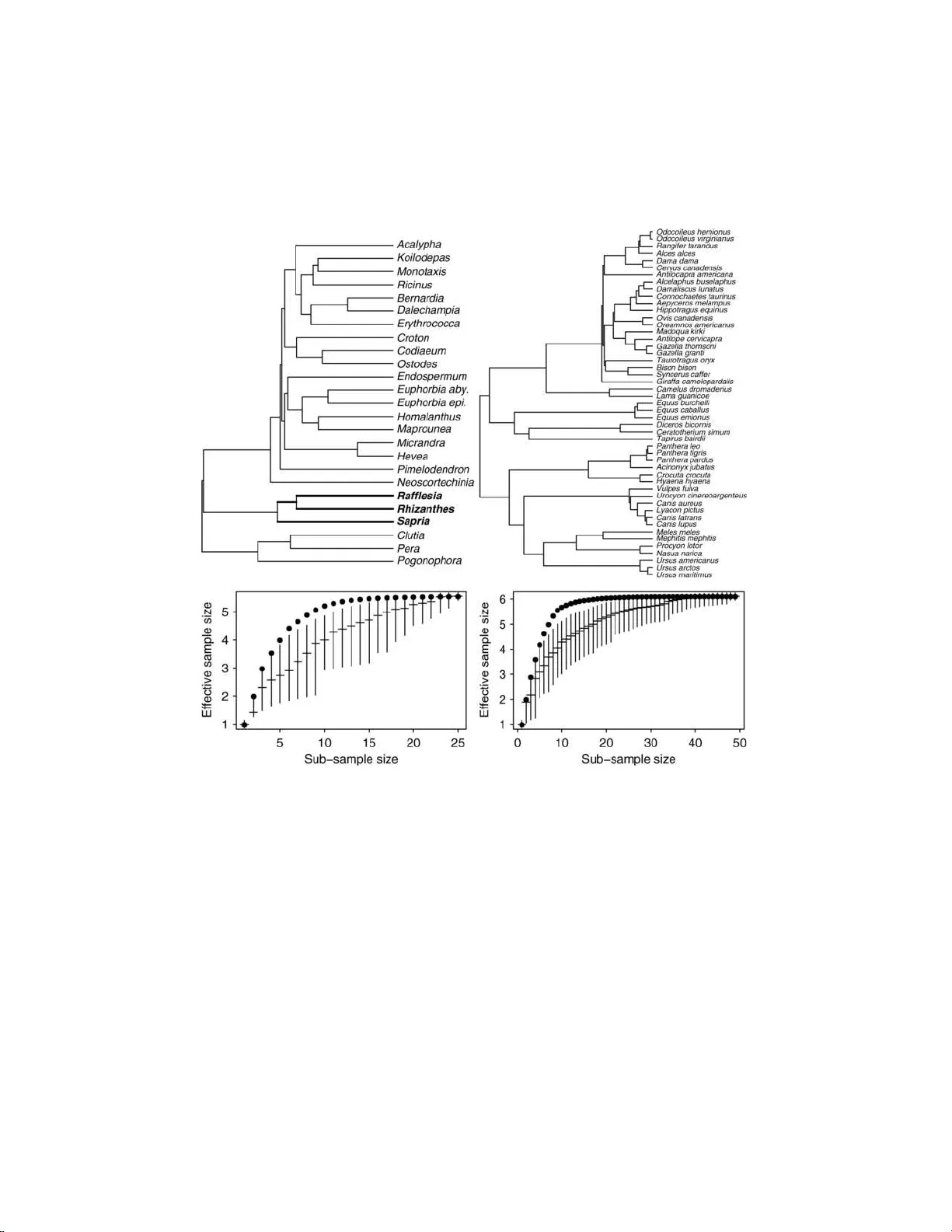
The Annals of Applie d Statistics 2008, V ol. 2, No. 3, 1078–110 2 DOI: 10.1214 /08-A OAS173 c  Institute of Mathematical Statistics , 2 008 ANAL YSIS OF COMP ARA TIVE D A T A WITH HIERAR C HICAL A UTOCORREL A TION By C ´ ecile An ´ e University o f Wisc onsin—Madison The asymptotic b ehavior of estimates and information criteria in linear mod els are studied in the context of hierarc hically correlated sampling units. The work is motiv ated by biological data collected on sp ecies where auto correlation is based on the species’ genealog- ical tree. Hierarc h ical autocorrelation is also found in many other kinds of data, such as from microarra y exp eriments or human lan- guages. Similar correlation also arises in ANOV A models with nested effects. I show that the b est linear unbiase d estimators are almost surely converg ent but ma y not be consistent for some p arameters such as the intercept and lineage effects, in the context of Brownian motion evol ution on the genealogical tree. F or the purp ose of mo del selection I sh ow that the usual BIC do es n ot provide an appropriate approximatio n to the p osterior probability of a mod el. T o correct for this, an effective sample size is introduced for parameters that are in- consisten tly estimated. F or biological studies, this w ork implies th at tree-aw are sampling design is d esirable; adding more sampling units ma y not help ancestral reconstruction and only strong lineage effects ma y b e detected with high p ow er. 1. In tro d uction. In man y ecolog ical or ev olutionary stud ies, scientists collect “comparativ e” data across biological sp ecies. It has long b een rec- ognized [ F elsenstei n ( 1985 )] that sampling u n its cannot b e considered inde- p endent in t his se tting. The reason i s that closely relate d sp ecies are ex- p ected to hav e similar c haracteristics, while a greater v ariabilit y is exp ected among distan tly related sp ecies. “Comparativ e metho ds” accoun ting f or an- cestry r elationships were first d ev elop ed and published in evo lu tionary b iol- ogy jour nals [ Harvey and P agel ( 1991 )], and are no w b eing used in v arious other fields. Indeed, h ierarc hical dep enden ce s tructures o f inherited tr aits arise in many areas, such as wh en sampling un its are genes in a gene family Received December 2007; revised Ap ril 2008. Key wor ds and phr ases. Asympt otic conv ergence, consistency , linear model, dep en- dence, comparative metho d, phylogenetic tree, Brownian motion evolution. This is an electronic r eprint of the origina l ar ticle published by the Institute of Mathematical Statistics in The Annals of Applie d Statistics , 2008, V ol. 2 , No. 3 , 1078 – 1102 . This reprint differs from the o riginal in pa gination and typogr a phic deta il. 1 2 C. AN ´ E Fig. 1. Example of a gene alo gic al tr e e f r om 4 units (l eft) and c ovarianc e matrix of ve ctor Y under the Br ownian motion mo del (right). [ Gu ( 2004 )], HIV virus samples [ Bhattac harya et al. ( 2007 )], human cul- tures [ Mace and Holden ( 200 5 )] or l anguages [ P agel, A tkinson and Meade ( 2007 )]. S u c h tree-structured units sh o w strong correlation, in some wa y similar to the correlation encount ered in spatial statistics. Und er the spa- tial “infi ll” asymptotic w here a region of s pace is filled in with d ensely sampled p oin ts, it is k n o wn that some parameters are n ot consisten tly es- timated [ Zhang and Zimmerman ( 2005 )]. It is sho w n here that inconsis- tency is also th e fate o f some paramete rs under hierarc hical dep endency . While spatial statistics is no w a well recognize d field, the statistical anal- ysis of tree-structured d ata has b een mostly dev elop ed b y biolog ists so far. This p ap er deals with a classical regression framework used to analyze data from h ierarc hically related sampling un its [ Martins and Hansen ( 1997 ), Housw orth , Martins and Lynch ( 2004 ), Garland, Bennett and Rezende ( 2005 ), Rohlf ( 2006 )]. Hier ar chic al auto c orr elation. Although sp ecies or genes in a gene fam- ily do n ot form an indep endent sample, their dep endence structure deriv es from their shared ancestry . Th e genealog ical relationships among the un its of interest are give n by a tree (e.g., Figure 1 ) wh ose br an ch lengths r epresen t some measure of ev olutionary time, most often c h ronological time. The r o ot of the tree represen ts a common ancestor to all units considered in the sam- ple. Metho ds for in f erring this tree t yp ically us e abundant molecular data and are no w extensiv ely dev elop ed [ F e lsenstein ( 2004 ), Semple and Steel ( 2003 )]. In this pap er the genealogic al tree relating the sampled units is assumed to b e kn o wn without error. The Bro wnian mo d el (BM) of ev olution states th at c haracters ev olve on the tree with a Bro wnian motion (Figure 2 ). After time t of ev olution, the c haracter is n ormally distributed, cent ered at the ancestral v alue at time 0 and with v ariance pr op ortional to t . Eac h in tern al no de in th e tree depicts a sp eciation ev ent : an ancestral lineage splitting int o t wo n ew lineages. The descendan t lineages inh er it the ancestral state ju st p rior to sp eciation. Eac h lineage th en ev olv es with an indep endent Bro w n ian motion. Th e co v ariance matrix of the data at the n tip s Y = ( Y 1 , . . . , Y n ) is then determined by the HIERARCHICAL AUTOCORRELA TION IN COMP ARA TIVE DA T A 3 tree and its b ranc h lengths: Y ∼ N ( µ, σ 2 V tree ) , where µ is the c haracter v alue at th e ro ot of the tree. Comp onents of V tree are the times of shared ancestry b et wee n tips, that is, V ij is the length shared by the p aths from the ro ot to the tip s i and j (Figure 1 ). T h e same structural cov ariance matrix could actually b e obtained un der other mo d els of ev olution, such as Bro wnian motion w ith drift, ev olution b y Gaussian jumps at r andom times or s tabilizing selection in a rand om en v ir onmen t [ Hansen and Martins ( 199 6 )]. Th e i.i.d. mo del is obtained w ith a “star” tree, w h ere all tips are dir ectly connected to the ro ot by edges of iden tical lengths. Another mo del of evo lu tion assumes an Orns tein–Uhlen b ec k (OU) pro cess and account s for stabilizing selectio n [ Hansen ( 1997 )]. T h e pr esen t pap er co vers th e assu mption of a BM structure of dep end ence, although sev eral results also app ly to OU and other mo dels. As th e Bro w nian motion is rev ersible, the tree can b e re-ro oted. When the ro ot is mo v ed to a new no de in the tree, the ancestral state µ represen ts the s tate of th e c haracter at that new no de, so re-ro oting the tr ee corresp onds to a re-parametrization. The line ar mo del. A f r equen t goal is to detect relationships b et ween tw o or more c haracters or to estimate ancestral traits [ Sc h luter et al. ( 1997 ), P agel ( 1999 ), Garland and Ives ( 2000 ), Huelsen b ec k and Bollbac k ( 2001 ), Blom b erg, Garland and Ives ( 2003 ), P agel, Meade and Bark er ( 2004 )]. In this pap er I consider th e linear mo del Y = X β + ε with ε ∼ N (0 , σ 2 V tree ) as derive d from a BM evol ution on the tree. When the matrix of predictors X is of fu ll rank k , it is wel l kno w n that the b est linear u nbiased estimator for β is ˆ β = ( X t V − 1 tree X ) − 1 X t V − 1 tree Y . Fig. 2. Si mulation of BM evolution along the tr e e in Fi gur e 1 . Anc estr al state was µ = 10 . Observe d values of Y ar e marke d by p oints. 4 C. AN ´ E Random co v ariates are t ypically assumed to ev olve with a BM on th e same tree as Y . Fixed cov ariates are also frequ en tly considered, such as deter- mined by a sub group of tips. Although th is mo del h as already b een us ed extensiv ely , the p resen t pa- p er is the first one to address its asymptotic prop erties. F or a meaningful asymptotic framewo rk, it is assumed that th e ro ot of the tree is fix ed w hile units are add ed to the sample. The reason is that th e in tercept relates to the ancestral state at the ro ot of the tree. If th e ro ot is pushed bac k in time as tips are added to the tree, then the meaning of th e in tercept change s and there is n o hop e of consistency for the in tercept. T he assum ption of a fixed ro ot is just a r o oting requirement. It do es not preven t an y unit to b e sampled. Asymptotic results assume the sample size go es to in finit y . I argue here that this is relev ant in real biological studies. F or instance, studies on phylo- genetical ly related viral samples hav e included hundreds of samples [ Bhattac hary a et al. ( 2007 )]. P agel, A tkins on and Meade ( 2007 ) ha ve bu ilt and used a tree relating as many as 87 Indo-Eur op ean languages. Man y groups count an incred ibly large n umb er of sp ecies. F or instance, there are ab out 20,000 orchid sp ecies to c ho ose fr om [ Dressler ( 1993 )], o ve r 10,000 sp ecies of b irds [ Jønsson and Fjelds ˚ a ( 2006 )], or ab out 20 0 wild p otato sp ecies [ Sp o oner and Hijmans ( 2001 )]. In add ition, studies can consider sub- p opulations and ev en individ u als w ithin sp ecies, so long as th ey are related b y a d iv ergent tree. Or ganization. The main results are illustrated on real examp les in Sec- tion 2 . It is sho w n that ˆ β is con verge n t almost sur ely and in L 2 norm in Section 3 . In Section 4 th en , I show that some comp onent s of ˆ β are not con- sisten t, con ve rging to some rand om v alue. T his is t ypically the case of the in tercept and of lineage effect estimators, while estimates of r andom co v ari- ate effects are consisten t. I in vestig ate a samp ling strategy—unrealistic for most biological settings—where consistency can b e ac hiev ed for the in ter- cept in S ection 4 . With this sampling strategy , I sh ow a phase transition for the rate of con vergence: if branc h es are not sampled close to the ro ot of the tree f ast en ou gh , the r ate of conv ergence is slo wer than the usual √ n r ate. In Section 5 I deriv e an appropriate formula for the Ba y esian Inform ation Criterion and int ro duce the concept of effectiv e sample size. Applications to biologica l problems are d iscussed in Section 6 , as w ell as app licatio ns to a broader cont ext of h ierarc hical mo dels s u c h as ANOV A. 2. Illustration of the m ain results. Da vis et al. ( 2007 ) analyzed flo wer size diameter f r om n = 25 sp ecies. Based on th e plan ts’ tree (Figure 3 left) assuming a simple BM m otion with no s hift, calculations yield an effectiv e sample size n e = 5 . 54 for the pur p ose of estimating flo wer diameter of the HIERARCHICAL AUTOCORRELA TION IN COMP ARA TIVE DA T A 5 ancestral s p ecies at th e ro ot. This is ab out a 4-fold decrease compared to the n u m b er of 25 sp ecies, resulting in a confidence interv al o v er 2 times wid er than otherwise exp ected fr om n = 25 i.i.d. sampling un its. The analysis of a larger tr ee with 49 sp ecies [ Garland et al. ( 1993 )] sho ws an 8-fold decrease with n e = 6 . 11. S ection 4 sho ws this is a general p henomenon: increasing th e sample size n cannot p ush th e effectiv e sample size n e asso ciated with the estimation of ancestral states b eyond some upp er b ound . More sp ecifically , Section 4 shows that n e ≤ k T / t , where k is the n u m b er of edges stemming from the ro ot, t is th e length of the shortest of these edges and T is the distance from the ro ot to the tips (or its a v erage v alue). T o accoun t for auto correlation, P aradis and Claude ( 2002 ) int ro duced a degree of freedom df P = L/T , where L is the s u m of all br anc h lengths. Int erestingly , n e is necessarily smaller than df P when all tips of the tree are at equal distance T from the ro ot (see App endix A ). Unexp ectedly large confidence inte rv als are already part of biologists’ ex- p erience [ Sc h luter et al. ( 1997 )]. As Cunningham, Omland an d Oakley ( 199 8 ) put it, likeli ho o d metho d s hav e “rev ealed a sur prising amount of un certain t y in ancestral reconstructions” to th e p oint th at authors ma y b e tempted to prefer metho d s that do not rep ort confid ence in terv als [ McArdle and Ro drigo ( 1994 )] or to ignore auto correlation due to shared ancestry [ Martins ( 2000 )]. Still, reconstructing ancestral states or detecting unusual shifts b et we en tw o ancestors are very fr equen t goals. F or example, Hansen ( 1997 ) hyp othesized a sh ift in to oth size to hav e o ccurred along the ancien t lineage separat- ing browsing h orses and grazing h orses. Recen t micro-arra y data from gene families ha v e in f erred ancestral exp r ession p atterns, as well as shifts that p ossibly o ccurred after genes w ere dup licated [ Gu ( 2004 )]. Guo et al. ( 2007 ) ha ve estimated sh ifts in brain growth along the human lin eage and along the lineage an cestral to human/c himp. Sections 3 and 4 show th at und er the BM m o del ancestral reconstructions and shift estimates are n ot consisten t, but are instead con vergen t tow ard a r andom limit. This is illustrated by small effectiv e sample sizes asso ciated with sh ift estimators. Among the 25 plan t sp ecies sampled by Da vis et al. ( 2007 ), 3 parasitic R afflesiac e ae sp ecies ha ve gigan tic flo wers (in b old in Figure 3 ). Un d er a BM mo del w ith a s hift on the R afflesiac e ae lineage, the effectiv e sample sizes for the ro ot’s state ( n e = 3 . 98) and for the s h ift ( n e = 2 . 72) are obtained from the R afflesiac e ae subtree and the remaining sub tree. T h ese low effectiv e sample sizes su ggest that only large sh if ts can b e detected w ith high p o wer. The p oten tial lac k of p ow er calls for optimal samplin g designs. T rees are t ypically b uilt from ab u ndant and relativ ely chea p molecular s equence data. More an d more often, a tree comprising many tips is a v ailable, w h ile traits of interest cannot b e collecte d f rom all tips on the tree. A c hoice h as to b e m ade on whic h tips shou ld b e kept for fur ther data collection. Until recen tly , inv estigato rs did not h a ve the tree at h and to mak e this c hoice, 6 C. AN ´ E Fig. 3. Phylo genetic tr e es fr om Davis et al. ( 2007 ) with 25 plant sp e cies, n e = 5 . 54 (left) and fr om Garland et al. ( 1993 ) with 49 mammal sp e cies, n e = 6 . 11 (right). Bottom: effe c- tive sample size n e for sub-samples of a gi ven size. V ertic al b ars indic ate 95% c onfidenc e interval and m e dian n e values when tips ar e sele cte d at r andom fr om the plant tr e e (left) and mammal tr e e (right). Dots indi c ate optimal n e values. but no w most inv estigators do. Therefore, optimal sampling design should use information from the tree. Figure 3 shows the effectiv e samp le size n e asso ciated with the r o ot’s state in the s imple BM m o del. First, sub-samples w ere formed by randomly selecting tip s and n e w as calculated for eac h s u b- sample. Since there can b e a huge num b er of combinations of tips, 1000 random sub-samp les of size k we r e generated for eac h k . Median and 95% confidence interv als for n e v alues are indicated b y vertica l bars in Figure 3 . Second, th e sub-samples of a size k that maximize the effectiv e sample size n e w ere obtained using step-wise backw ard and forward searc hes. Both HIERARCHICAL AUTOCORRELA TION IN COMP ARA TIVE DA T A 7 searc h strategies agreed on the same maximal n e v alues, which are indicated with d ots in Figure 3 . F rom b oth trees, only 15 tips suffice to obtain a near maximum effectiv e sample size, pro vid ed that the selected tip s are w ell c h osen, n ot rand omly . T he pr op osed selection of tips m aximizes n e and is based on the phylog eny on ly , pr ior to data collection. I n v iew of the b ound for n e men tioned ab o ve , the selected tips will tend to retain the k edges stemming from the ro ot and to m inimize the length of these edges b y retaining as man y of the early branching lineages as p ossible. F or the p urp ose of mo del selection, BIC is widely u sed [ Sc hw arz ( 1978 ), Kass and Raftery ( 1995 ), Butler and Kin g ( 2004 )] and is usually defined as − 2 ln L ( ˆ β , ˆ σ ) + p log( n ) , where L ( ˆ β , ˆ σ ) is the maximized lik eliho o d of the mo del, p the num b er of parameters and n the num b er of observ ations. E ac h parameter in the mo del is th u s p enalized b y a log( n ) term. Section 6 sh o ws that this form u la do es n ot p r o vide an approxi mation to the mo d el p osterior probabilit y . Instead, the p enalty asso ciated with the in tercept and with a shift should b e b ound ed, and log (1 + n e ) is an app r opriate p enalt y to b e used for eac h inconsisten t parameter. On the plant tree, the in tercept (ancestral v alue) sh ou ld therefore b e p en alized b y log (1 + 5 . 54) in the simple BM mo del. In the BM mo del that includes a shift along the p arasitic p lan t lineage, th e in tercept should b e p enalized b y ln(1 + 3 . 98) and the shift by ln(1 + 2 . 72 ). These p enalties are AIC -lik e (b oun ded) for high-v ariance p arameters. 3. Con vergence of estimators. Th is section prov es the conv ergence of ˆ β = ˆ β ( n ) as th e sample size n increases. The assumption of a fixed ro ot implies that the co v ariance matrix V tree = V n (indexed b y the sample size) is a s u bmatrix of V n +1 . Theorem 1. Consider the line ar mo del Y i = X i β + ε i with ε ( n ) = ( ε 1 , . . . , ε n ) t ∼ N (0 , σ 2 V n ) and wher e pr e dictors X may b e e i ther fixe d or r andom. Assume the design matrix X ( n ) (with X i for i th r ow) is of ful l r ank pr ovide d n is lar ge enough. Then the e stimator ˆ β n = ( X ( n ) t V n − 1 X ( n ) ) − 1 X ( n ) t V n − 1 Y ( n ) is c onver gent almost sur ely and in L 2 . Comp onent ˆ β n,j c onver ges to the true value β j if and only if its asymptot ic varianc e is zer o. Otherwise, it c onver ges to a r andom variable ˆ β ∗ j , which dep ends on the tr e e and the actual data. Note th at no assump tion is made on th e co v ariance s tr ucture V n , except that it is a s ubmatrix of V n +1 . Therefore, T heorem 1 holds r egardless of ho w the sequence V n is selected. F or instance, it holds f or the OU mo del, wh ose co v ariance matrix has comp onen ts V ij = e − αd ij or V ij = (1 − e − 2 αt ij ) e − αd ij (dep endin g whether the ancestral state is conditioned u p on or integ r ated 8 C. AN ´ E out), where d ij is the tr ee d istance b etw een tips i and j , and α is the kno w n selection strength. Theorem 1 can b e viewe d as a str on g la w of large n umbers: in the absence of co v ariates and in the i.i.d. case ˆ β n is ju s t the s amp le mean. Here, in the absence of co v ariates ˆ β n is a wei gh ted a ve rage of the observ ed v alues, estimating the ancestral state at the ro ot of the tree. Sampling un its close to the ro ot could b e provided by f ossil sp ecies or by early viral samples wh en sampling s pans seve ral y ears. Suc h units, close to the ro ot, wei gh more in ˆ β n than units furth er a wa y fr om the ro ot. Th eorem 1 giv es a la w of large n u m b er for this wei gh ted av erage. Ho wev er, w e will see in S ection 4 that the limit is random: ˆ β n is inconsistent. Pr oof of Theore m 1 . The pro cess ε = ( ε 1 , ε 2 , . . . ) is well d efined on a probabilit y space Ω b ecause the co v ariance m atrix V n is a submatrix of V n +1 . Deriv ations b elo w are made conditional on the predictors X . In a Ba y esian-lik e approac h, the probabilit y space is expanded to e Ω = R k × Ω by considering β ∈ R k as a random v ariable, indep endent of errors ε . Assume a p riori that β is normally distr ib uted w ith mean 0 and co v ariance matrix σ 2 I k , I k b eing the ident it y matrix of size k . Let F n b e the fi ltration gener- ated by Y 1 , . . . , Y n . Sin ce β , Y 1 , Y 2 , . . . is a Gaussian p ro cess, the conditional exp ectation E ( β |F n ) is a linear com bin ation of Y 1 , . . . , Y n up to a constan t: E ( β |F n ) = a n + M n Y ( n ) . The almost su re con v erge of ˆ β n will follo w from the almost sure con verge nce of the martingale E ( β |F n ) and from id entifying M n Y ( n ) with a linear trans- formation of ˆ β n . Th e vect or a n and matrix M n are su ch that E ( β |F n ) is the pro jection of β on F n in L 2 ( e Ω), that is, these co efficien ts are su c h that trace( E ( β − a n − M n Y ( n ) )( β − a n − M n Y ( n ) ) t ) is minimum. Since Y i = X i β + ε i , β is cen tered and indep end en t of ε , w e get that a n = 0 and the quantit y to b e m inimized is tr(( I k − M n X ( n ) ) v ar( β )( I k − M n X ( n ) ) t ) + tr( M n v ar( ǫ ( n ) ) M t n ) . The m atrix M n app ears in the first term th rough M n X ( n ) , so we can m ini- mize σ 2 tr( M n V n M t n ) u n der the constraint that B = M n X ( n ) is fixed. Using Lagrange m ultipliers, we get M n V n = Λ X ( n ) t sub ject to M n X ( n ) = B . As- suming X ( n ) t V − 1 n X ( n ) is inv ertible, it follo ws Λ = B ( X ( n ) t V − 1 n X ( n ) ) − 1 and M n Y ( n ) = B ˆ β ( n ) . The minimum attained is then σ 2 tr( B ( X ( n ) t V − 1 n X ( n ) ) − 1 B t ). This is necessarily smaller than σ 2 tr( MV n M t ) wh en M is formed by M n − 1 and an add itional column of zeros. So for an y B , the trace of B ( X ( n ) t V − 1 n X ( n ) ) − 1 B t HIERARCHICAL AUTOCORRELA TION IN COMP ARA TIVE DA T A 9 is a decreasing sequence. Since it is also nonnegativ e, it is conv ergen t and so is ( X ( n ) t V − 1 n X ( n ) ) − 1 . No w the quadratic expression tr(( I k − B )( I k − B ) t ) + tr( B ( X ( n ) t V − 1 n X ( n ) ) − 1 B t ) is min im ized if B satisfies B ( I k + ( X ( n ) t V − 1 n X ( n ) ) − 1 ) = I k . Note the symm et- ric definite p ositive matrix I k + ( X ( n ) t V − 1 n X ( n ) ) − 1 w as sho wn ab o v e to b e decreasing with n . In sum mary , E ( β |F n ) = ( I k + ( X ( n ) t V − 1 n X ( n ) ) − 1 ) − 1 ˆ β ( n ) . This martingale is b ound ed in L 2 ( e Ω) so it con verges almost surely and in L 2 ( e Ω) to E ( β |F ∞ ). Finally , ˆ β ( n ) − β = ( I k + ( X ( n ) t V − 1 n X ( n ) ) − 1 ) E ( β |F n ) − β is also con vergen t almost surely and in L 2 ( e Ω). But ˆ β n − β is a f unction of ω in the original probabilit y space Ω, in d ep endent of β . Therefore, for an y β , ˆ β ( n ) con verge s almost surely and in L 2 (Ω). S ince ε is a Gaussian p ro cess, the limit of ˆ β ( n ) is normally distribu ted with co v ariance matrix the limit of ( X ( n ) t V − 1 n X ( n ) ) − 1 . It follo ws that ˆ β ( n ) k , whic h is unbiased, con verge s to the true β k if and only if the k th d iagonal element of ( X ( n ) t V − 1 n X ( n ) ) − 1 go es to 0.  4. Consistency of estimators. In this section I pro ve b ounds on the v ari- ance of v arious effects ˆ β i . F rom Theorem 1 we know that ˆ β i is strongly consisten t if and only if its v ariance go es to zero. 4.1. Inter c ept. Assume h ere that the first column of X is the column 1 of ones, and the first comp onen t of β , the intercept, is d enoted β 0 . Pr oposition 2. L et k b e the numb er of daughters of the r o ot no de, and let t b e the length of the shortest br anch stemming fr om the r o ot. Then v ar( ˆ β 0 ) ≥ σ 2 t/k . In p articular, when the tr e e is binary we have v ar( ˆ β 0 ) ≥ σ 2 t/ 2 . The follo win g inconsistency r esu lt follo ws directly . Corollar y 3. If ther e is a lower b ound t > 0 on the length of br anches stemming f r om the r o ot, and an upp e r b ound on the numb e r of br anches stemming fr om the r o ot, then ˆ β 0 is not a c onsistent estimator of the inter c ept, even though it is unbi ase d and c onver gent. The conditions ab ov e are v ery natural in m ost biological settings, since most ancient lineages ha v e gone extinct. The lo w er b ound ma y b e pushed do wn if abund an t fossil data is a v ailable or if ther e has b een adaptiv e r adi- ation w ith a bur st of sp eciation ev ents at the r o ot of the tree. 10 C. AN ´ E Pr oof of Pr oposition 2 . Assum in g the linear mo del is correct, the v ariance of ˆ β is giv en b y v ar( ˆ β ) = σ 2 ( X t V − 1 X ) − 1 , where th e first column of X is the vecto r 1 of ones, so that the v ariance of the inte rcept estimator is just the fi rst diagonal elemen t of σ 2 ( X t V − 1 X ) − 1 . But ( X t V − 1 X ) − 1 ii ≥ ( X i t V − 1 X i ) − 1 for any index i [ Rao ( 1973 ), 5a.3, page 327], so th e pr o of can b e reduced to the simp lest case with no co v ariates: Y i = β 0 + ε i . Th e basic idea is that the information p ro vid ed by all the tips on the ancestral state β 0 is no more than the information p ro vided just b y the k direct d escendan ts of the ro ot. Let us consider Z 1 , . . . , Z k to b e the c h aracter s tates at the k branc hes stemming f rom th e ro ot after a time t of ev olution (Figure 4 , left). These s tates are not observ ed, but the observed v alues Y 1 , . . . , Y n ha ve ev olv ed from Z 1 , . . . , Z k . No w I claim that the v ariance of ˆ β 0 obtained from the Y v alues is no smaller than the v ariance of ˆ β ( z ) 0 obtained from the Z v alues. S ince the Z v alues are i.i.d. Gaussian w ith mean β 0 and v ariance σ 2 t , ˆ β ( z ) 0 has v ariance σ 2 t/k . T o pr o ve the claim, consider β 0 ∼ N (0 , σ 2 ) indep end en t of ǫ . Th en E ( β 0 | Y 1 , . . . , Y n , Z 1 , . . . , Z k ) = E ( β 0 | Z 1 , . . . , Z k ) so that v ar( E ( β 0 | Y 1 , . . . , Y n )) ≤ v ar( E ( β 0 | Z 1 , . . . , Z k )). Th e pro of of Th eorem 1 shows that E ( β 0 | Y 1 , . . . , Y n ) = ˆ β 0 / (1 + t y ) wh ere t y = ( 1 t V − 1 1 ) − 1 so, sim- ilarly , E ( β 0 | Z 1 , . . . , Z k ) = ˆ β ( z ) 0 / (1 + t z ) where t z = t /k . Since β 0 and ˆ β 0 − β 0 are indep endent, the v ariance of E ( β 0 | Y 1 , . . . , Y n ) is ( σ 2 + t y σ 2 ) / (1 + t y ) 2 = σ 2 / (1 + t y ). Th e v ariance of E ( β 0 | Z 1 , . . . , Z k ) is obtained similarly and we get 1 / (1 + t y ) ≤ 1 / (1 + t z ), that is, t y ≥ t z and v ar( ˆ β 0 ) = σ 2 ( 1 t V − 1 1 ) − 1 ≥ σ 2 t/k .  4.2. Line age eff e ct. This section considers a p redictor X 1 that defin es a sub tree, that is, X 1 i = 1 if tip i b elongs to the sub tree and 0 otherwise. This is similar to a 2-sample comparison problem. Th e t yp ical “treatmen t” effect corresp onds here to a “lineage” effect, the lineage b eing the b r anc h subtendin g th e subtree of in terest. If a shift o ccurred along that lineage, Fig. 4. L eft: O bserve d states ar e Y 1 , . . . , Y n , whil e Z 1 , . . . , Z k ar e the unobserve d states along the k e dges br anching fr om the r o ot, after time t of evolution. Y pr ovides less information on β 0 than Z . Right: Z 0 , Z 1 , . . . , Z k top ar e unobserve d states pr oviding mor e information on the line age effe ct β 1 than the observe d Y values. HIERARCHICAL AUTOCORRELA TION IN COMP ARA TIVE DA T A 11 Fig. 5. Mo del M 0 (left) and M 1 (right) with a l ine age effe ct. X 1 is the indic ator of a subtr e e. Mo del M 1 c onditions on the state at the subtr e e’s r o ot, mo di fying the dep endenc e structur e. tips in th e subtree will tend to hav e, sa y , high trait v alues relativ e to the other tips. Ho w ever, the BM mo del do es pr edict a c han ge, on an y branch in the tree. So the question is whether the actual sh ift on the lineage of in terest is compatible with a BM c h ange, or whether it is to o large to b e solely exp lained b y Bro wnian motion. Alternativ ely , one might just estimate the actual c h ange. This consideration leads to t wo mod els. In the first m o del, a shift β 1 = β ( S ) top is add ed to the Br ownian motion c h ange along the branch of in terest, so that β ( S ) top represent s the characte r displacement not d ue to BM n oise. In th e second mo del, β 1 = β ( S B ) top is the actual change , whic h is the su m of the Brownian motion noise and an y extra shift. Observ ations are then conditioned on the actual an cestral states at the r o ot and the sub tr ee’s r o ot (Figure 5 ). By the Marko v p rop erty , observ ations from the tw o subtrees are conditionally ind ep endent of eac h other. In the second mo del then, th e co v ariance matrix is mo difi ed. The mo dels are wr itten Y = 1 β 0 + X 1 β 1 + · · · + X k β k + ε with β 1 = β ( S ) top and ε ∼ N (0 , σ 2 V tree ) in the first mo del, wh ile β 1 = β ( S B ) top and ε ∼ N (0 , σ 2 diag( V top , V bot )) in the second mo d el, where V top and V bot are the co v ariance matrices asso ciated with the top and b ottom su btrees obtained by r emo ving the br anc h su b tending the group of int erest (Figure 5 ). Pr oposition 4. L e t k top b e the numb er of br anches stemming fr om the subtr e e of inter est, t top the length of the shortest br anch stemming f r om the r o ot of this subtr e e , and t 1 the length of the br anch subtending the subtr e e. Then v ar( ˆ β ( S ) top ) ≥ σ 2 ( t 1 + t top /k top ) and v ar( ˆ β ( S B ) top ) ≥ σ 2 t top /k top . Ther efor e, if t top /k top r emains b ounde d fr om b elow when the sample size incr e ases, b oth e stimators ˆ β ( S ) top (pur e shift) and ˆ β ( S B ) top (actual change) ar e inc onsistent. 12 C. AN ´ E F rom a p ractical p oin t of view, unless f ossil data is a v ailable or there w as a radiation (bur st of sp eciation even ts) at b oth ends of the lineage, shift estimators are n ot consistent. Increasing the sample size m igh t not help detect a shift as m u c h as one wo uld typical ly exp ect. Note that the pur e shift β ( S ) top is confoun d ed w ith the Bro wn ian noise, so it is no w onder that this quantit y is not identifiable as so on as t 1 > 0. The adv an tage of the first mo del is that the BM w ith n o additional shift is n ested within it. Pr oof of Proposition 4 . In b oth mo d els v ar( ˆ β 1 ) is the second d iago- nal element of σ 2 ( X t V − 1 X ) − 1 whic h is b oun ded b elo w b y σ 2 ( X 1 t V − 1 X 1 ) − 1 , so that w e need just pro ve the result in the s implest mo d el Y = β 1 X 1 + ε . Similarly to Prop osition 2 , defin e Z 1 , . . . , Z k top as the charact er states at the k top direct descendants of the sub tree’s r o ot after a time t top of ev olution. Also, let Z 0 b e the state of n o de just paren t to the sub tree’s ro ot (see Fig- ure 4 , r igh t). Like in Prop osition 2 , it is easy to see that the v ariance of ˆ β 1 giv en the Y is larger than the v ariance of ˆ β 1 giv en the Z 0 , Z 1 , . . . , Z k top . In the s econd mo del, β 1 = β ( S B ) top is the actual state at th e subtree’s ro ot, so Z 1 , . . . , Z k top are i.i.d. Gaussian centered at β ( S B ) top with v ariance σ 2 t top and the result follo ws easily . In the first mo del, the state at th e subtree’s ro ot is the s u m of Z 0 , β ( S ) top and the BM noise along the lineage, so ˆ β ( S ) top = ( Z 1 + · · · + Z k top ) /k top − Z 0 . This estimate is the sum of β ( S ) top , the BM noise and the sampling error ab out the subtree’s ro ot. The result follo ws b ecause the BM n oise and sampling error are in d ep endent w ith v ariance σ 2 t 1 and σ 2 t top /k top resp ectiv ely .  4.3. V arianc e c omp onent. In con trast to th e inte rcept and lineage effects, inference on th e r ate σ 2 of v ariance accum ulation is straight forw ard . An unbiase d estimate of σ 2 is ˆ σ 2 = R S S / ( n − k ) = ( b Y − Y ) t V − 1 tree ( b Y − Y ) / ( n − k ) , where b Y = X ˆ β are pr edicted v alues and n is the num b er of tips. The classical indep end ence of ˆ σ 2 and ˆ β still holds for any tree, and ( n − k ) ˆ σ 2 /σ 2 follo ws a χ 2 n − k distribution, k b eing th e rank of X . I n particular, ˆ σ 2 is u n b iased and con verge s to σ 2 almost su rely as the samp le size increases, as sh o wn in App end ix B . Although n ot surpr ising, this b ehavio r con trasts with the inconsistency of the interce pt and lineage effect estimators. W e k eep in mind , ho wev er, that the conv er gence of ˆ σ 2 ma y not b e robust to a violation of the normalit y assumption or to a missp ecification of the dep en d ence structure, either fr om a inadequate mo del (BM v ersu s O U) or f rom an error in the tree. HIERARCHICAL AUTOCORRELA TION IN COMP ARA TIVE DA T A 13 4.4. R andom c ovariate effe cts. In this section X denotes the matrix of random co v ariates, exclud in g the v ector of ones or any subtree indicator. In most cases it is reasonable to assume that r an d om co v ariates also follo w a Bro wnian motion on the tree. Co v ariates ma y b e corr elated, accum ulating co v ariance t Σ on an y single edge of length t . Then co v ariates j and k ha ve co v ariance Σ j k V tree . With a sligh t abuse of notation (considering X as a single large v ector), v ar( X ) = Σ ⊗ V tree . Pr oposition 5. Consider Y = 1 β 0 + X β 1 + ε with ε ∼ N (0 , σ 2 V tree ) . Assume X fol lows a Br ownian evolution on the tr e e with nonde gener ate c ovarianc e Σ : X ∼ N ( µ X , Σ ⊗ V tree ) . Then v ar( ˆ β 1 ) ∼ σ 2 Σ − 1 /n asymptot- ic al ly. In p articular, ˆ β 1 estimates β 1 c onsistently b y The or em 1 . R andom c ovariate effe cts ar e c onsistently and e ffic i ently estimate d, even though the inter c ept is not. Pr oof. W e ma y wr ite V − 1 = R t R using the Cholesky decomp osition for example. Since R1 6 = 0, we ma y find an orthogonal m atrix O s uc h that OR1 = ( a, 0 , . . . , 0) t for some a , so without loss of generalit y , w e may assume that R1 = ( a, 0 , . . . , 0) t . Th e mo del no w b ecomes R Y = R1 β 0 + RX β 1 + R ε , where er r ors R ε are n o w i.i.d. Let e X 0 b e the firs t r o w of RX and let e X 1 b e the matrix made of all but th e firs t row of RX . Similarly , let ( ˜ y 0 , e Y t 1 ) t = R Y and ( ˜ ε 0 , ˜ ε t 1 ) t = R ε . The mo d el b ecomes e Y 1 = e X 1 β 1 + ˜ ε 1 , ˜ y 0 = aβ 0 + e X 0 β 1 + ˜ ε 0 with least square solution ˆ β 1 = ( e X t 1 e X 1 ) − 1 e X t 1 e Y 1 = β 1 + ( e X t 1 e X 1 ) − 1 e X t 1 ˜ ε 1 and ˆ β 0 = ( ˜ y 0 − e X 0 ˆ β 1 ) /a . T he v ariance of ˆ β 1 conditional on X is then σ 2 ( e X t 1 e X 1 ) − 1 . Using the condition on R1 , th e ro ws of e X 1 are i.i.d. cen tered Gaussian with v ariance-co v ariance Σ and ( e X t 1 e X 1 ) − 1 has an in - v erse Wishart distribution w ith n − 1 degrees of fr eedom [ Johnson and Kotz ( 1972 )]. The u nconditional v ariance of v ar( ˆ β 1 ) is then σ 2 E ( e X t 1 e X 1 ) − 1 = σ 2 Σ − 1 / ( n − k − 2) , where k is the n umber of rand om co v ariates, which completes the pro of.  Remark. The result still h olds if one or more lineage effects are in- cluded an d if the m o del conditions up on th e c h aracter state at eac h sub tree (second mo d el in S ection 4.2 ). Th e reason is that data fr om eac h subtree are indep end en t, and in eac h su btree th e mo del h as ju st an in tercept in addition to the random cov ariates. The b eha vior of r andom effect estimators contrasts with the b eha v ior of the interce pt or lineage effect estimators. An intuitiv e explanation might b e the follo w in g. Eac h cherry in the tree (pair of adj acen t tips) is a pair of siblings. Eac h pair pr o vides indep endent evidence on the c hange of Y and of X b et wee n the 2 siblings, ev en though parent al information is u na v ail- able. E v en though means of X and Y are p o orly known, there is abu ndant 14 C. AN ´ E evidence on ho w they c h ange with eac h other. S im ilarly , the metho d of ind e- p endent con trasts [ F elsenstein ( 1985 )] identifies n − 1 i.i.d. pair-like c h anges. 5. Phase transition for symmetric trees. T he motiv ation for this section is to determin e the b eha vior of the in tercept estimator wh en branches can b e sampled closer and closer to th e ro ot. I sh o w that the intercept can b e consisten tly estimated, although the rate of conv ergence can b e muc h slo wer than ro ot n . The f o cus is on a sp ecial case with symmetric sampling (Figure 6 ). The tree h as m leve ls of in tern al no des with the r o ot at lev el 1. All no des at lev el i share the s ame d istance f r om the ro ot t 1 + · · · + t i − 1 and the same num b er of descendant s d i . In a binary tree all internal no des ha v e 2 descendan ts and the sample size is n = 2 m . The total tree heigh t is set to 1, that is, t 1 + · · · + t m = 1. With these symm etries, the eigen v alues of the cov ariance matrix V n can b e completely determined (see App endix C ), smaller eigen v alues b e- ing associated with shallo wer in ternal n o des (close to the tips) and larger eigen v alues b eing asso ciated w ith more b asal no des (close to the ro ot). In particular, the constan t v ector 1 is an eigen ve ctor and ( 1 t V n 1 ) − 1 = t 1 /d 1 + · · · + t m / ( d 1 . . . d m ). In order to sample br an ches close to the ro ot, consid er replicating th e ma jor b ranc h es stemming from the ro ot. Sp ecifically , a prop ortion q of eac h of these d 1 branc hes is ke pt as is by the ro ot, and the other pr op ortion 1 − q is replicated along w ith its subtendin g tree (Figure 6 ), that is, t ( m ) 1 = q m − 1 and t ( m ) i = (1 − q ) q m − i for i = 2 , . . . , m . F or simplicit y , assume further that groups are replicated d ≥ 2 times at eac h step, that is, d 1 = · · · = d m = d . Fig. 6. Symm etric sampling (left) and r epli c ation of major br anches close to the r o ot (right). HIERARCHICAL AUTOCORRELA TION IN COMP ARA TIVE DA T A 15 The r esult b elo w sh o ws a la w of large n u m b ers and p r o vides the rate of con verge n ce. Pr oposition 6. Consider the mo del with an inter c ept and r andom c o- variates Y = 1 β 0 + X β 1 + ε with ε ∼ N (0 , σ 2 V n ) on the symmetric tr e e describ e d ab ove. Then ˆ β 0 is c onsistent. The r ate of c onver genc e exp erienc es a phase tr ansition dep ending on how close to the r o ot new br anches ar e adde d: v ar( ˆ β 0 ) is asymptotic al ly pr op ortional to n − 1 if q < 1 /d , ln( n ) n − 1 if q = 1 /d or n α if q > 1 /d wher e α = ln( q ) / ln( d ) . Ther efor e, the r o ot- n r ate of c onver genc e is obtaine d as in the i.i.d. c ase if q < 1 /d . Conver genc e is much slower if q > 1 /d . Pr oof. By Theorem 1 , th e consistency of ˆ β 0 follo ws from its v ariance going to 0. First consider the mo d el with no co v ariates. Up to σ 2 , the v ari- ance of ˆ β 0 is ( 1 t V n 1 ) − 1 = t 1 /d 1 + · · · + t m / ( d 1 . . . d m ), wh ich is q m − 1 /d + (1 − q )(1 − ( q d ) m − 1 ) / ( d m (1 − q d )) if q d 6 = 1 and (1 + (1 − q )( m − 1)) /d m if q d = 1. Th e result follo w s easily since n = d m , m ∝ ln( n ) and q m = n α . In the p resence of r andom cov ariates, it is easy to see that th e v ariance of ˆ β 0 is incr eased by v ar( ˆ µ X ( ˆ β 1 − β 1 )), where ˆ µ X = e X 1 /a is the ro w ve ctor of the co v ariates’ estimated ancestral s tates (using notations fr om the pr o of of Prop osition 5 ). By Prop osition 5 this increase is O ( n − 1 ), wh ic h completes the p r o of.  6. Ba yesian information criterion. The b asis for using BIC in m o del selection is that it p ro vides a go o d appro ximation to the marginal mo d el probabilit y giv en the d ata and given a prior distribu tion on th e parameters when the sample size is large. Th e pro of of this pr op ert y u ses the i.i.d. assumption quite hea vily , and is b ased on the lik eliho o d b eing more and more p eak ed around its maxim u m v alue. Here, h o wev er, th e like liho o d do es not concen trate around its maximum v alue since ev en an infinite sample size ma y conta in little in formation ab out some parameters in the m o del. The follo wing prop osition shows that the p enalt y associated with the interce pt or with a lineage effect ought to b e b ound ed, th us smaller than log ( n ). Pr oposition 7. Consider k r andom c ovariates X with Br ownian evo- lution on the tr e e and nonsingular c ovarianc e Σ , and the line ar mo dels Y = β 0 1 + X β 1 + ε with ε ∼ N (0 , σ 2 V tree ) (M 0 ) Y = β 0 1 + X β 1 + β top 1 top + ε with ε ∼ N (0 , σ 2 V tree ) , (M 1 ) wher e the line age factor 1 top is the indic ator of a (top) subtr e e . Assume a smo oth prior distribution π over the p ar ameters θ = ( β , σ ) and a sampling such that 1 t V − 1 n 1 is b ounde d, that is, br anches ar e not sample d to o close 16 C. AN ´ E fr om the r o ot. With mo del M 1 assume further that br anches ar e not sample d to o close fr om the line age of inter est, that i s, 1 t top V − 1 n 1 top is b ounde d. Then for b oth mo dels, the mar ginal pr ob ability of the data P ( Y ) = R P ( Y | θ ) π ( θ ) dθ satisfies − 2 log P ( Y ) = − 2 ln L ( ˆ θ ) + ( k + 1) ln( n ) + O (1) as the sample size incr e ases. Ther efor e, the p enalty for the inter c ept and for a line age e ff e ct is b ounde d as the sample size incr e ases. The p o orly estimated parameters are not p enalized as sev erely as the consisten tly estimated p arameters, since they lead to only small or mo derate increases in lik eliho o d. Also, the p rior information contin ues to influ ence the p osterior of the data ev en with a ve ry large sample size. Note that th e lineage effect β top ma y either b e the pu re sh if t or the actual c hange. Mo del M 0 is nested w ithin M 1 in the first case only . In the p ro of of Prop osition 7 (see Ap p endix D ) the O (1) term is sh o wn to b e dominated b y C = log d et ˆ Σ − ( k + 1) log (2 π ˆ σ 2 ) + log 2 + D , where D dep ends on the mo del. In M 0 D = − 2 log Z β 0 exp( − ( β 0 − ˆ β 0 ) 2 / (2 t 0 ˆ σ 2 )) π ( β 0 , ˆ β 1 , ˆ σ ) dβ 0 , (1) where t 0 = lim( 1 t V − 1 n 1 ) − 1 . In M 1 D = − 2 log Z β 0 ,β top exp( − ˜ β t W − 1 ˜ β / (2 ˆ σ 2 )) π ( β 0 , β top , ˆ β 1 , ˆ σ ) dβ 0 dβ top , (2) where ˜ β t = ( β 0 − ˆ β 0 , β top − ˆ β top ) and the 2 × 2 symmetric m atrix W − 1 has diagonal element s lim 1 t V − 1 n 1 = t − 1 0 , lim 1 t top V − 1 n 1 top < ∞ and off-diagonal elemen t lim 1 t V − 1 n 1 top , whic h do es exist. In the rest of the section I assume that all tips are at the same d istance T from the ro ot. Th is condition is realized wh en branch lengths are chrono- logica l times an d tips are sampled simulta neously . Under BM, Y 1 , . . . , Y n ha ve common v ariance σ 2 T . Th e ancestral state at the ro ot is estimated with asymptotic v ariance σ 2 / lim n 1 t V − 1 n 1 , w hile the same precision wo uld b e obtained with a sample of n e indep end en t v ariables w here n e = T lim n 1 t V − 1 n 1 . Therefore, I call this quan tit y the effe ctive sample size asso ciated w ith the in tercept. The next prop osition pr ovides more accuracy for the p enalt y term in case the p rior h as a sp ecific, reasonable form. In some s ettings, it h as b een shown HIERARCHICAL AUTOCORRELA TION IN COMP ARA TIVE DA T A 17 that the err or term in the BIC approximat ion is actually b etter than O (1). Kass and W asserman ( 1995 ) sho w this error term is only O ( n − 1 / 2 ) if the prior carries the same amount of information as a sin gle obser v ation w ould, as w ell as in the context of comparing nested m o dels w ith an alternativ e h y - p othesis close to the n ull. I follo w Kass and W asserman ( 1996 ) and consider a “reference prior” that con tains little inform ation, lik e a single observ ation w ould [see also Raftery ( 1995 , 1996 ), W asserman ( 2000 )]. In an emp irical Ba y es wa y , assume the pr ior is Gaussian cen tered at ˆ θ . L et ( β 1 , σ ) ha ve prior v ariance J − 1 n = diag ( ˆ σ 2 ˆ Σ − 1 , ˆ σ 2 / 2) and b e in dep endent of the other parameter(s) β 0 and β top . Also, let β 0 ha ve v ariance ˆ σ 2 T in mo del M 0 . In mo del M 1 , assum e further that the tree is ro oted at the base of the lineage of int erest, so that the int ercept is the ancestral state at the base of that lineage. T his r ep arametrizatio n has the adv antage that ˆ β 0 and ˆ β 0 + ˆ β top are uncorrelated asymp toticall y . A single observ ation from outside the subtree of int erest (i.e., fr om the b ottom subtree) would b e cen tered at β 0 with v ariance σ 2 T , while a single observ ation f r om the top su btree would b e cen tered at β 0 + β top with v ariance σ 2 T top . In case β top is the p ure s hift, then T top = T . If β top is the actual change along the lineage, then T top is the heigh t of the su btree excluding its subtending br anc h. Therefore, it is reasonable to assign ( β 0 , β top ) a prior v ariance of ˆ σ 2 W π with W π =  T − T − T T + T top  . The only tips in forming β 0 + β top are those in the top subtr ee and the only units inf orm ing β 0 are those in the b ottom subtree. Therefore, the effectiv e sample sizes asso ciated with the inte r cept and lineage effects are defin ed as n e, b ot = T lim n 1 t V − 1 bot 1 , n e, top = T top lim n 1 t V − 1 top 1 , where V bot and V top are the v ariance matrices from the b ottom and top subtrees. Pr oposition 8. Consider mo dels M 0 and M 1 and the prior sp e cifie d ab ove. Then P ( Y | M 0 ) = − 2 ln L ( ˆ θ | M 0 ) + ( k + 1) ln( n ) + ln(1 + n e ) + o (1) and P ( Y | M 1 ) = − 2 ln L ( ˆ θ | M 1 ) + ( k + 1) ln( n ) + ln(1 + n e, b ot ) + ln(1 + n e, top ) + o (1) . Ther efor e, a r e asonable p enalty for the nonc onsistently estimate d p ar ameters is the lo g of their effe ctive sample sizes plus one. Pr oof. With mo del M 0 , w e get from ( 1 ) D = − 2 log π ( ˆ β 1 , ˆ σ ) − 2 log Z exp  − ( β 0 − ˆ β 0 ) 2 2 t 0 ˆ σ 2 − ( β 0 − ˆ β 0 ) 2 2 T ˆ σ 2  dβ 0 √ 2 π T ˆ σ = − 2 log π ( ˆ β 1 , ˆ σ ) + log(1 + T /t 0 ) . 18 C. AN ´ E No w − 2 log π ( ˆ β 1 , ˆ σ ) = ( k + 1) log (2 π ) − log det J n cancels with th e first con- stan t terms to give C = log (1 + T /t 0 ) = log (1 + n e ). With mo del M 1 , we get D = − 2 log π ( ˆ β , ˆ σ ) − 2 log det( W − 1 + W − 1 π ) − 1 / 2 det W 1 / 2 π , so that again C = log (det( W − 1 + W − 1 π ) det W π ). It remains to iden tify this quan tit y with ln(1 + n e, b ot ) + ln(1 + n e, top ). It is easy to see that det W π = T T top and W − 1 π =  T − 1 + T − 1 top T − 1 top T − 1 top T − 1 top  . Since V is blo ck d iagonal diag ( V top , V bot ), we h a ve that 1 t V − 1 1 top = n e, top /T top and 1 t V − 1 1 = 1 t V − 1 top 1 + 1 t V − 1 bot 1 = n e, top /T top + n e, b ot /T . T h erefore, W − 1 has diagonal terms n e, top /T top + n e, b ot /T and n e, b ot /T top and off-diagonal term n e, b ot /T top . W e get det( W − 1 + W − 1 π ) = ( n e, b ot + 1) /T top ( n e, b ot + 1) /T , whic h completes the p ro of.  Akaike’s information criterion (AIC). This criterion [ Ak aike ( 1974 )] is also widely used for mo del selection. With i.i.d. samples, AIC is an estimate of the Kullbac k–Leibler dive rgence b et ween the tru e distribution of the data and the estimated distribution, up to a constan t [ Burnham and Anderson ( 2002 )]. Because of th e BM assum ption, the Ku llbac k–Leibler d iv ergence can b e calculated explicitly . Using the Gaussian distribu tion of the d ata, the m u tual in dep enden ce of ˆ σ 2 and ˆ β and the chi-square distr ib ution of ˆ σ 2 , the usual deriv ation of AIC applies. Contrary to BIC, the AIC appro ximation still h olds with tree-structure d ep endence. 7. Applications and d iscussion. This pap er p ro vides a la w of large n um- b ers for non i.i.d. sequences, whose dep enden ce is go verned by a tree struc- ture. Almost s u re con v ergence is obtained, but the limit ma y or ma y not b e the exp ected v alue. With s p atial or temp oral data, the correlation d e- creases rapidly with sp atial distance or with time t ypically (e.g., AR pro- cesses) und er expand in g asymptotics. With a tr ee structur e, the d ep endence of an y 2 new ob s erv ations from 2 giv en sub trees w ill h a ve the s ame corre- lation with eac h other as with “older” ob s erv ations. In spatial statistics, infill asymptotics also h arb or a strong, nonv anishing correlation. T his de- p endence implies a b ounded effect iv e sample size n e in most realistic b io- logica l settings. Ho wev er, I sho wed that th is effectiv e sample size p ertains to lo cations parameters only (in tercept, lineage effects). Inconsistency has also b een describ ed in p opulation genetics. In particular, T a jima’s estima- tor of the lev el of sequence div ers it y from a s amp le of n in dividuals is not HIERARCHICAL AUTOCORRELA TION IN COMP ARA TIVE DA T A 19 consisten t [ T a jima ( 1983 )], wh ile asymptotically optimal estimators only con verge at rate log( n ) rather than n [ F u and Li ( 1993 )]. T he r eason is that the genealogic al correlation among individ u als in the p opulation decreases the av ailable information. Sampling design. V ery large genealogies are no w a v ailable, with h un- dreds or thou s ands of tips [ Cardillo et al. ( 2005 ), Bec k et al. ( 2006 )]. It is not uncommon that ph y s iologi cal, morp hological or other phen otypic data cannot b e measured for all units in the group of in terest. F or the pu r p ose of estimating an ancestral state, the samp ling s trategy su ggested here max- imizes the scaled effectiv e sample size 1 t V − 1 n 1 ov er all subsamp les of size n , where n is an affordable n umb er of units to subsample. This criterion is a function of the r o oted tree top ology and its br an ch lengths. It is very easy to calculate with one tree trav ersal using F elsenstein’s algorithm [ F elsenstein ( 1985 )], w ithout in v erting V n . It might b e computationally too costly to as- sess all su b samples of size n , but one might heuristically searc h only among the most star-lik e su b trees. Bac kward and forw ard stepwise searc h strategies w ere implemented, either removing or add ing tips one at a time. Desp e r ate situation? T his pap er pro vides a theoretical explanation for the kno wn difficult y of estimating ancestral states. In terms of detecting non- Bro wnian shifts, our results imply that the maxim um p ow er cann ot reac h 100%, ev en with infin ite sampling. Ins tead, w hat mostly drive s the p o w er of shift detection is the effect size: β 1 / √ tσ wh ere β 1 is the shift size and t is the length of the lineage exp eriencing the s hift. T h e situation is desp erate only in cases w hen the effect size is small. Incr eased sampling ma y not provide more p o wer. Beyond the Br ownian motion mo del. The con verge nce result applies to an y dep endence matrix. Bounds on the v ariance of estimates do not apply to the Or nstein–Uhlen b ec k mo d el, so it w ould b e in teresting to study the consistency of estimates in this mo del. Ind eed, wh en selectio n is strong the OU pro cess is attracted to the optimal v alue and “forgets” the initial v alue exp onent ially fast. Several studies ha v e clearly indicated that some ancestral states and lineage-sp ecific optimal v alues are not estimable [ Butler and King ( 2004 ), V erd ´ u and Gleiser ( 2006 )], thus b earing on the question of h o w effi- cien tly these p arameters can b e estimated. While th e OU mo del is already b eing us ed , theoretical questions remain op en. Br o ader hier ar chic al auto c orr elation c ontext. So far lin ear mod els w ere considered in th e cont ext of biological data with sh ared ancestry . Ho wev er, implications of this work are far reac hing and ma y affect common p r actices 20 C. AN ´ E Fig. 7. T r e es asso ciate d with ANOV A mo dels: 3 gr oups with fixe d effe cts (left) or r andom effe cts (right). V arianc e within and among gr oups ar e σ 2 e and σ 2 a r esp e ctively. in man y fi elds, b ecause tree structured auto correlation und er lies man y ex- p erimenta l designs. F or in stance, the typical ANOV A can b e repr esented b y a forest (with BM ev olution), one star tree for eac h group (Figure 7 ). If groups ha ve random effects, then a single tree captures this mo del (Figure 7 ). It shows visually ho w the v ariation decomp oses in to w ith in and among group v ariation. ANOV A with several n ested effects w ould b e represen ted b y a tree with more hierarc h ical lev els, eac h no d e in the tree repr esen ting a group. In suc h r andom (or mixed) effect mo dels, asymptotic r esu lts are kno wn when the num b er of groups b ecomes large, while the num b er of un its p er group is not necessarily required to gro w [ Akritas and Arnold ( 2000 ), W ang and Akritas ( 2004 ), G ¨ uve n ( 2006 )]. Th e resu lts p resen ted h er e p ertain to any kind of tr ee gro w th, even when grou p sizes are b oun d ed. Mo del sele ction. Man y asp ects of the mo del can b e selected for, such as the most imp ortant pr edictors or the appropr iate dep end ence stru cture. Moreo v er, there often is some uncertaint y in the tree structur e or in the mo del of ev olution. Several trees migh t b e obtained from molecular d ata on sev eral genes, for instance. These trees m ight hav e differen t top ologies or just differen t sets of branc h lengths. BIC v alues from s everal tr ees can b e com bined for m o del a ve raging. I show ed in this pap er that the standard f orm of BIC is inapp r opriate. Instead, I prop ose to adj u st the p enalt y asso ciated to an estimate with its effectiv e sample size. AIC w as sh o wn to b e still appropriate f or approximat ing the Kullb ack– Leibler criterion. Op e n q u estions. It wa s shown th at the scaled effectiv e sample s ize is b ound ed as long as the n u m b er k of edges stemming fr om the ro ot is b ound ed and their lengths are ab o ve some t > 0. The con verse is not true in general. T ake a star tree with edges of length n 2 . Then Y n ∼ N ( µ, σ 2 n 2 ) are in d e- p endent, and 1 t V − 1 n 1 = P n − 2 is b oun ded. How ev er, if one requires that the tree height is b ounded (i.e., tips are d istan t from the ro ot by no more than a m axim um amount ), then is it necessary to ha ve k < ∞ and t > 0 for the effectiv e sample size to b e b ound ed? If not, it w ould b e in teresting to know a necessary condition. HIERARCHICAL AUTOCORRELA TION IN COMP ARA TIVE DA T A 21 APPENDIX A: UPPER BOUND F OR THE EFFECT IVE SAMPLE SIZE I pro ve here the claim made in Section 2 that the effectiv e sample size for the intercept n e = T 1 t V − 1 1 is b ounded by df P = L/T , where L is the tree length (the sum of all br anc h lengths), in case all tips are at equal distance T from the ro ot. I t is easy to see that V is blo ck diagonal, eac h blo c k corresp ondin g to one s u btree b ranc h ing f r om the ro ot. Therefore, V − 1 is also b lo c k d iagonal and, by in duction, we only need to sh o w that n e ≤ L /T when the ro ot is adjacent to a single edge. Let t b e the length of this edge. When this edge is prun ed from the tree, one obtains a subtr ee of length L − t and whose tips are at distance T − t from the ro ot. Let V − t b e the co v ariance matrix asso ciated with this su btree. By induction, one ma y assum e that 1 t V − t 1 ≤ ( L − t ) / ( T − t ) 2 . No w V is of the form t J + V − t , wh ere J = 11 t is a square matrix of ones. It is easy to c heck that V − 1 1 = V − 1 − t 1 / (1 + t 1 t V − 1 − t 1 ) so that 1 t V − 1 1 = (( 1 t V − 1 − t 1 ) − 1 + t ) − 1 ≤ (( T − t ) 2 / ( L − t ) + t ) − 1 . By conca vity of the inv erse f unction, ((1 − λ ) /a + λ/b ) − 1 < (1 − λ ) a + λb for all λ in (0 , 1) and all a > b > 0. Combining the t wo p revious inequalities with λ = t/T , a = ( L − t ) / ( T − t ) and b = 1 yields 1 t V − 1 1 < L/T 2 and pr o ve s th e claim. The equalit y n e = df P only o ccur s w hen the tree is reduced to a sin gle tip, in whic h case n e = 1 = d f P . APPENDIX B: ALMO S T SURE CONVERG ENCE OF ˆ σ AND ˆ Σ Con vergence of ˆ σ in pr ob ab ility is obtained b ecause ν ˆ σ 2 n /σ 2 has a c h i- square distribution with degree of f r eedom ν = n − r , r b eing the total n u m b er of co v ariates. Th e exact kno wledge of this distribution p ro vides b ound s on tail p robabilities. Strong conv ergence f ollo ws from the conv er - gence of the series P n P ( | ˆ σ 2 n − σ 2 | > ε ) < ∞ for all ε > 0, w hic h in tur n follo ws from the app licatio n of Chern o v’s b oun d and d eriv ation of large deviations [ Dem b o and Zeitouni ( 1998 )]: P ( ˆ σ 2 − σ 2 > ε ) ≤ exp( − ν I ( ε )) and P ( ˆ σ 2 − σ 2 < − ε ) ≤ exp( − ν I ( − ε )) where the r ate function I ( ε ) = ( ε − log (1 + ε )) / 2 f or all ε > − 1 is obtained fr om the moment generating function of th e chi-square distribution. The co v ariance matrix of random effects is estimated with ν ˆ Σ n = e X t 1 e X 1 = ( X − ˆ µ X ) t V − 1 n ( X − ˆ µ X ), with e X 1 as in the pr o of of Prop osition 5 , whic h has a Wishart d istribution with degree of freedom ν = n − 1 and v ariance parameter Σ . F or eac h ve ctor c then, c t ν ˆ Σ n c has a c hi-square distribu tion with v ariance p arameter c t Σc , so that c t ˆ Σ n c conv erges almost su rely to c t Σc by th e ab o ve argumen t. Using the ind icator of th e j th co ordinate c = 1 j , then c = 1 i + 1 j , w e obtain the strong con vergence of ˆ Σ to Σ . 22 C. AN ´ E APPENDIX C: SYMMETRIC T REES With the symmetric samp ling from Section 5 , eigen v alues of V n are of the form λ i = n  t i d 1 . . . d i + · · · + t m d 1 . . . d m  with multiplicit y d 1 . . . d i − 1 ( d i − 1) , the num b er of no d es at lev el i if i ≥ 2. A t the ro ot (lev el 1) the multiplicit y is d 1 . Indeed, it is easy to exhibit the eigen v ectors of eac h λ i . Consid er λ 1 for ins tance. The d 1 descendan ts of the ro ot define d 1 groups of tips. If v is a v ector suc h that v j = v k for tips j and k is the same group , then it is easy to see that V n v = λ 1 v . It shows that λ 1 is an eigen v alue with m ultiplicit y d 1 (at least). No w consider an in tern al no de at lev el i . Its d escendan ts form d i groups of tips, which we name G 1 , . . . , G d i . Let v b e a v ector suc h that v j = 0 if tip j is not a descendant of the no d e and v j = a g if j is a descendant from group g . Then , if a 1 + · · · + a d i = 0 , it is easy to see that V n v λ i v . Since the multiplic ities sum to n , all eigen v alues and eigen vecto rs h a ve b een iden tified. APPENDIX D: BIC APPRO XIMA TION Pr oof of Proposition 7 . The prior π is assumed to b e s ufficien tly smo oth (four times con tinuously differentia ble) and b ound ed. Th e same con- ditions are also required for π m defined b y π m = s up β 0 π ( β 1 , σ | β 0 ) in mo del M 0 and π m = s up β 0 ,β top π ( β 1 , σ | β 0 , β top ) in mo del M 1 . Th e extra assum p tion on π m is prett y mild; it holds when parameters are in d ep endent a priori, f or instance. F or mo del M 0 the lik eliho o d can b e written − 2 log L ( θ ) = − 2 log L ( ˆ θ ) + n  ˆ σ 2 σ 2 − 1 − log ˆ σ 2 σ 2  + (( β 1 − ˆ β 1 ) t X t V − 1 n X ( β 1 − ˆ β 1 ) + 1 t V − 1 n 1 ( β 0 − ˆ β 0 ) 2 + 2( β 0 − ˆ β 0 ) 1 t V − 1 n X ( β 1 − ˆ β 1 )) /σ 2 . Rearranging terms, we get − 2 log L ( θ ) = − 2 log L ( ˆ θ ) + 2 nh n ( θ ) + a n ( β 0 − ˆ β 0 ) 2 / ˆ σ 2 , where a n = 1 t V − 1 n 1 − 1 t V − 1 n X ( X t V − 1 n X ) − 1 X t V − 1 n 1 , 2 h n ( θ ) =  ˆ σ 2 σ 2 − 1 − log ˆ σ 2 σ 2  + ( β 1 − u 1 ) t X t V − 1 n X nσ 2 ( β 1 − u 1 ) + a n n ( β 0 − ˆ β 0 ) 2  1 σ 2 − 1 ˆ σ 2  and u 1 = ˆ β 1 − ( β 0 − ˆ β 0 )( X t V − 1 n X ) − 1 X t V − 1 n 1 . F or any fixed v alue of β 0 , consider h n as a fu nction of β 1 and σ . Its minim u m is attained at u 1 and HIERARCHICAL AUTOCORRELA TION IN COMP ARA TIVE DA T A 23 ˆ σ 2 1 = ˆ σ 2 + a n ( β 0 − ˆ β 0 ) 2 /n . A t this p oint the minimum v alue is 2 h n ( u 1 , ˆ σ 1 ) = log(1 + a n ( β 0 − ˆ β 0 ) 2 / ( n ˆ σ 2 )) − a n ( β 0 − ˆ β 0 ) 2 / ( n ˆ σ 2 ) and the second deriv ative of h n is J n = d iag( X t V − 1 n X / ( n ˆ σ 2 1 ) , 2 / ˆ σ 2 1 ). Note that ˆ µ X = 1 t V − 1 n X / ( 1 t V − 1 n 1 ) is the ro w v ector of estimated ancestral states of X , so by Theorem 1 , it is con verge nt. Note also that X t V − 1 n X = ( n − 1) ˆ Σ + ( 1 t V − 1 n 1 ) µ X t µ X . Since 1 t V − 1 n 1 is assumed b oun ded, X t V − 1 n X = n ˆ Σ + O (1) almost surely , and the error term dep ends on X only , n ot on the parameters β or σ . Consequently , a n = 1 t V − 1 n 1 + O ( n − 1 ) is almost surely b ound ed and ˆ σ 2 1 = ˆ σ 2 + O ( n − 1 ). I t follo ws th at for any fi xed β 0 , J n con verge s almost sur ely to diag( Σ /σ 2 , 2 /σ 2 ). Therefore, its eigen v alues are almost surely b ounded and b oun ded a w ay from zero, and h n is Laplace-regular as defined in Kass, Tierney an d Kadane ( 1990 ). Theorem 1 in Kass, T ierney and Kadane ( 1990 ) sho ws that − 2 log Z e − nh n π dβ 1 dσ = 2 nh n ( u 1 , ˆ σ 1 ) + ( k + 1) log n + log det ˆ Σ 1 − ( k + 1) log (2 π ˆ σ 2 1 ) + log 2 − 2 log( π ( ˆ β 1 , ˆ σ | β 0 ) + O ( n − 1 )) with ˆ Σ 1 = X t V − 1 n X /n = ˆ Σ + O ( n − 1 ). In tegrating fur ther o ver β 0 , we get − 2 log P ( Y ) = − 2 log L ( ˆ θ ) + ( k + 1) log n + log d et ˆ Σ 1 − ( k + 1) log (2 π ˆ σ 2 ) + log 2 + D n , wh ere D n = − 2 log Z exp  − n − k − 1 2 log  1 + a n ( β 0 − ˆ β 0 ) 2 n ˆ σ 2  × ( π ( ˆ β 1 , ˆ σ | β 0 ) + O ( n − 1 )) π ( β 0 ) dβ 0 . Heuristically , we see that a n con verge s to t − 1 0 = lim 1 t V − 1 n 1 an d for fi xed β 0 the integ rand is equiv alen t to exp( − ( β 0 − ˆ β 0 ) 2 / (2 t 0 ˆ σ 2 )), s o w e w ould con- clude that D n con verge s to D = − 2 log R exp( − ( β 0 − ˆ β 0 ) 2 / (2 t 0 ˆ σ 2 )) π ( β 0 , ˆ β 1 , ˆ σ ) dβ 0 as giv en in ( 1 ) and , thus, − 2 log P ( Y ) = − 2 log L ( ˆ θ ) + ( k + 1) log n + log det ˆ Σ − ( k + 1) log (2 π ˆ σ 2 ) + log 2 + D + o (1) . F ormally , we need to c h ec k that the O ( n − 1 ) term in D n has an o (1) cont ri- bution after integ ration, and that the limit of the in tegral is th e integ r al of the p oin t-wise limit. T he int egrand in D n is the pro du ct of f n ( β 0 ) = n ( k +1) / 2 Z exp(log L ( θ ) − log L ( ˆ θ )) π ( β 1 , σ | β 0 ) dβ 1 dσ and of a quantit y that conv erges almost surely: (2 det ˆ Σ 1 ) 1 / 2 (2 π ˆ σ 2 ) − ( k + 1) / 2 . Maximizing the lik eliho o d and prior in β 0 , we get that f n is u niformly 24 C. AN ´ E b ound ed in β 0 b y n ( k +1) / 2 Z exp  − n 2  ˆ σ 2 σ 2 − 1 − log ˆ σ 2 σ 2 + ( β 1 − ˆ β 1 ) t ˆ Σ 2 ( β 1 − ˆ β 1 ) /σ 2  × π m ( β 1 , σ ) dβ 1 dσ , where ˆ Σ 2 = ( XV − 1 n X − 1 t V − 1 n 1 ˆ µ t X ˆ µ X ) /n con verge s almo st surely to Σ . Since π m is assumed smo oth and b ou n ded, w e can apply Theorem 1 from Kass, T iern ey and K adane ( 1 990 ) again, and f n ( β 0 ) is b ounded b y (2 det ˆ Σ 2 ) − 1 / 2 (2 π ˆ σ 2 ) ( k +1) / 2 × π m ( ˆ β 1 , ˆ σ ) w hic h is a conv ergen t qu antit y . There- fore, f n is uniform ly b oun ded an d b y dominated con ve rgence, the limit of R f n π dβ 0 equals the inte gral of the p oin t-wise limit so that D n = D + o (1) as claimed in ( 1 ). F or mo del M 1 the pro of is similar. The v alue u 1 is no w ˆ β 1 − ( X t V − 1 n X ) − 1 (( β 0 − ˆ β 0 ) X t V − 1 n 1 + ( β top − ˆ β top ) X t V − 1 n 1 top ) . The term a n ( β 0 − ˆ β 0 ) 2 is r eplaced by e β t A n e β , where e β t = ( β 0 − ˆ β 0 , β top − ˆ β top ) and A n is the 2 × 2 sym m etric ma- trix with diagonal elemen ts a n and 1 t top V − 1 1 top − 1 t top V − 1 X ( X t V − 1 X ) − 1 X t V − 1 1 top , and off-diagonal element 1 t V − 1 1 top − 1 t V − 1 X ( X t V − 1 X ) − 1 X t V − 1 1 top . Note that, as b efore, elemen ts in A n are dominated by their fir st term, since X t V − 1 X = n Σ + O (1) almost surely . I s ho w b elo w that A n con verge s to W − 1 as defined in ( 2 ), whose elemen ts are the limits of 1 t V − 1 n 1 , 1 t top V − 1 n 1 top and 1 t V − 1 n 1 top . The first quant it y is t − 1 0 , fin ite by assump tion. The second qu an tit y equals 1 t e V − 1 1 , where e V is obtained by p r uning the tree from all tips not in the top subtr ee, so it con- v erges and is n ecessarily smaller than t − 1 0 . Th e third quan tit y exists b ecause ( 1 t V − 1 n 1 ) − 1 ( 1 t V − 1 n 1 top ) is ˆ µ top , the estimated state at the ro ot fr om char- acter 1 top . Theorem 1 cannot b e ap p lied to show its con v ergence, b ecause 1 top is a n onrandom c haracter, b ut conv ergence f ollo ws fr om the follo win g facts: (a) ˆ µ top is the estimated state at th e ro ot from a tree where the top subtree is r educed to a single “top” leaf w hose su btending b r anc h length decreases when more tips are added to the top subtree, to a nonn egativ e limit. (b) On the redu ced tree, ˆ µ top is the w eigh t with whic h the top leaf con tribu tes to ancestral state estimation. (c) This w eight d ecreases as more tips are added outside the top sub tree.  Ac kn o wledgment s. Th e author is very grateful to Thomas Kurtz for in- sigh tfu l discus sions on the almost su re con v ergence result. REFERENCES Akaike, H. ( 1974). A new look at t he statistical mo del identification. I EEE T r ans. Au- tomat. Contr ol 19 716–723 . MR0423716 HIERARCHICAL AUTOCORRELA TION IN COMP ARA TIVE DA T A 25 Akrit as, M. and Arnold, S. (2000). Asymptotics for analysis of v ariance when the num b er of levels is large. J. Amer. Statist. Asso c. 95 212–226. MR1803150 Beck, R . M. D., Bi ninda-Emonds, O. R. P., Cardillo, M., Li u, F.-G. R. and Pur vis, A. (2006). A higher-level MRP sup ertree of p lacen tal mammals. BMC Evol. Biol. 6 93. Bha tt achar y a, T., Daniels, M., H eckerman, D., Foley, B., Frahm, N., Kadie, C., Carlson, J., Yusim, K., McMahon, B., Gaschen, B. , M a llal, S., Mullins, J., Ni ckle, D., Herbeck, J., Roussea u , C., Learn, G., Miura, T. , Bra nder, C. , W alker, B. D. and Korber, B. (2007). F ounder effects in th e assessment of HI V p olymorphisms and hla allele asso ciations. Scienc e 315 1583–158 6. Blomberg, S. P., Ga rland, Jr., T. and Ives, A. R. ( 2003). T esting for phylogenetic signal in comparative data: b eh a v ioral traits are more labile. Evolution 57 717–745. Burnham, K. P. and Ande rson, D. R. (2002). Mo del sele ction and mul ti m o del i nfer enc e: A Pr actic al Information-The or etic Appr o ach , 2nd ed . Sp ringer, New Y ork. MR1919620 Butler, M. A. and King, A. A. (2004). Ph ylogenetic comparative analysis: A mo deling approac h for adaptive evolution. The Americ an Natur alist 164 683–69 5. Cardillo, M., Mace, G. M. , Jones, K. E., B ielby, J., Bi ninda-Emonds, O. R. P., Se chrest, W ., Orme, C. D. L. and Pur vis, A. (2005). Multiple cau ses of high extinction risk in large mammal sp ecies. Scienc e 309 1239–1241. Cunningham , C. W., Omland, K. E. and Oakley, T. H. (1998). Reconstru cting ances- tral chara cter states: a critical reappraisal. T r ends in Ec olo gy and Evolution 13 361–366. Da vis, C . C., La tvis, M., Nickrent, D. L., Wurda ck, K. J. and Baum, D. A. (2007). Floral gigantism in Rafflesiaceae. Scienc e 315 1812. Dembo, A . and Zeitouni, O. (1998). L ar ge Deviations T e chniques and Appli c ations , 2nd ed. S pringer, New Y ork. MR1619036 Dressler, R. L. (1993). Phylo geny and Classific ation of the Or chid F amil y . Dioscorides Press, US A. Felsenstein, J. (1985). Phylog enies and the comp arative method . The Americ an Natu- r alist 125 1–15. Felsenstein, J. (2004). Inferring Phylo genies . S inauer Asso ciates, Sunderland, MA. Fu, Y.-X. and Li , W.-H. (1993). Maximum likeli hoo d estimation of p opulation parame- ters. Genetics 134 1261–1270. Garland, T. , Jr., Bennett, A. F. and Rezend e, E. L. (2005). Phylogenetic approaches in comparative physiology. J. Exp erimental Bi olo gy 208 3015–3 035. Garland, T., Jr., Dickerman, A . W., Janis, C. M. and Jones, J. A. (1993). Phylo- genetic analysis of cov ariance by computer sim u lation. Systematic Bi olo gy 42 265–292. Garland, T., Jr. and Ive s, A. R. (2000). Using the past to predict the present: Con- fidence interv als for regressi on equations in phyloge netic comparative metho ds. The Amer ic an Natur ali st 155 346–364. Gu, X. (2004). Statistical framework for phylogenomic analysis of gene family expression profiles. Genetics 167 531–542. Guo, H., We i ss, R. E., Gu, X . and Suchard, M. A. (2007). Time squ ared: R ep eated measures on phylogenies. Mole cular Biolo gy Evolution 24 352–362. G ¨ uven, B. (2006). The limiting d istribution of the F-statistic from n onnormal universes. Statistics 40 545–557. MR2300504 Hansen, T. F. (1997). S tabilizing selection and the comparative analysis of adaptation. Evolution 51 1341–1 351. Hansen, T. F. and Mar tins, E. P. (1996). T ranslating b etw een microevolutionary pro- cess and macro evo lutionary patterns: The correlation structure of interspecific data. Evolution 50 1404–1 417. 26 C. AN ´ E Har vey, P. H . and P agel, M. (1991). The Comp ar ative Metho d in Evolutionary Bi olo gy . Oxford Univ. Press. Housw or th, E. A., Ma r tins, E. P. and L ynch, M. (2004). The phylog enetic mixed mod el. The Amer ic an Natur ali st 163 84–96. Huelsenbeck, J. P. and B ollba ck, J. (2001). Empirical and hierarc h ical Ba yesian es- timation of ancestral states. Systematic Biolo gy 50 351–366. Johnson, N. L. and Kotz, S. (1972). D i stributions in Statistics: Continuous Multivariate Distributions . Wiley , New Y ork. MR0418337 Jønsson, K. A. and Fjelds ˚ a, J. (2006). A phylogenetic sup ertree of oscine p asserine birds ( Aves: Passeri). Zo ologica S cripta 35 149–186 . Kass, R. E. and Rafter y, A. E. (1995). Bay es factors. J. A mer. Statist. Asso c. 90 773–795 . Kass, R. E., Tiern ey, L. and Kadane, J. B. (1990). The v alidit y of p osterior exp an - sions based on Laplace’s metho d. In Bayesian and Likeliho o d metho ds in Statistics and Ec onometrics 473–488. North- Holland, Amsterdam. Kass, R. E. and W asserm an, L. (1995). A reference Ba yesian test for nested hyp otheses and its relationship to the S c hw arz criterion. J. Amer . Statist. Asso c. 90 928–934 . MR1354008 Kass, R. E. and W asserman, L. (1996). The selection of p rior distribut ions by formal rules. J. Amer. Statist. Asso c. 91 1343–1370. Mace, R. and Holden, C. J. (2005). A phylo genetic approach to cultural evolution. T r ends in Ec olo gy and Evolution 20 116–121. Mar tins, E. P. (2000). A daptation and the comparative metho d. T r ends in Ec olo gy and Evolution 15 296–29 9. Mar tins, E. P. and Hansen, T. F. (1997). Phylogenies and the comparative metho d: A general approac h to incorp orating p hyloge netic information in to the analysis of inter- sp ecific data. The Americ an Natur alist 149 646–667. McArdle, B. and Rodrigo, A. G. (1994). Estimati ng the ancestral states of a conti nuous-v alued character using squ ared-change parsimon y : An analytical solution. Systematic Biolo gy 43 573–578. P agel, M. (1999). The maximum likelihoo d approach to reconstructing ancestral charac - ter states of discrete characters on phylogenies . Systematic Biolo gy 48 612–62 2. P agel, M ., A tkinson, Q. D. and Mead e, A. (2007). F requency of word-use predicts rates of lexical evol ution throughout ind o- europ ean history . Natur e 449 717–720. P agel, M ., Meade , A. and Barker, D. (2004). Ba yesian estimation of ancestral char- acter states on phylogenies. Systematic Biolo gy 53 673–684. P ara dis, E. and Claude, J. (2002). Analysis of comparativ e data using generalized estimating eq uations. J. The or et. Bi olo gy 218 175–18 5. MR2027281 Rafter y, A. E. (1995). Ba yesian mod el selection in so cial researc h. So ciolo gic al Metho d- olo gy 25 111–163 . Rafter y, A. E. ( 1996). Approximate Bay es factors and accounting for mo del un certainty in generalised linear mo dels. Biometrika 83 251–266. MR1439782 Rao, C . R. (1973). Line ar Statistic al Infer enc e and Its Applic ations , 2n d ed. Wiley , New Y ork. MR0346957 Ro hlf, F. J. (2006). A comment on phylogenetic regression. Evolution 60 1509–151 5. Schluter, D., Price, T., Mooers, A. O. and Ludwig, D. (1997). Likelihood of ancestor states in adaptive radiation. Evolution 51 1699–1711. Schw arz, G. (1978). Estimating th e dimension of a mod el. Ann. Statist. 6 461–464. MR0468014 HIERARCHICAL AUTOCORRELA TION IN COMP ARA TIVE DA T A 27 Semple, C. and Steel, M. (2003). Phylo genetics . Ox ford Un iv. Press, New Y ork. MR2060009 Spooner, D. M. and H i jmans, R. J. (2001). Potato systematics and germplasm collect- ing, 1989-2000 . Americ an J. Potato R ese ar ch 78 237–268; 395. T ajima, F. (1983). Ev olutionary relationship of DNA sequences in fin ite p opulations. Genetics 105 437–460. Verd ´ u, M. and G leiser, G. (2006). A daptive evolution of reprodu ctive an d vegetativ e traits driven by breeding systems. New Phytolo gi st 169 409–417. W ang, H. and Akrit as, M. (2004). Rank tests for ANOV A with large number of factor leve ls. J. Nonp ar ametr. Stat. 16 563–589. MR2073042 W asserman, L. (2000). Ba yesi an mo del selection and mo del av eraging. J. Math. Psych. 44 92–107. MR1770003 Zhang, H. and Zimme rman, D. L. (2005). T o w ards reconciling tw o asymptotic frame- w ork s in spatial statistics. Biom etrika 92 921–936. MR2234195 Dep ar tments of S t a tistics and of Bot any University of Wisconsin—Madison 1300 University A venue Madison, Wisconsin 53706 USA E-mail: ane@stat.wisc.edu