Evolving Neural Networks through a Reverse Encoding Tree

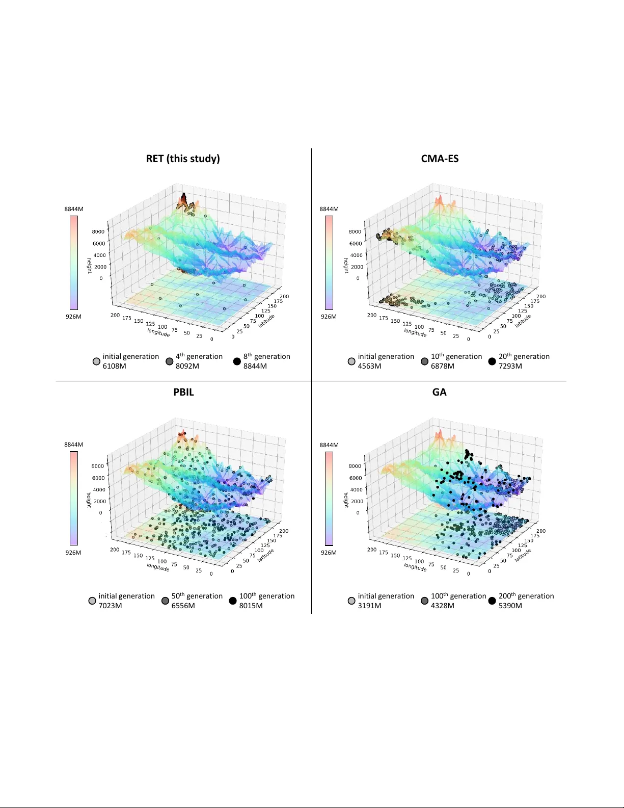
Ev olving Neural Networks through a Re v erse Encoding T ree Haoling Zhang Chao-Han Huck Y ang Hector Zenil Narsis A. Kiani Institute of Biochemistry School of ECE Algorithmic Dynamics Lab & Algorithmic Dynamics Lab BGI-Shenzhen Geor gia Institute of T echnolo gy Oxfor d Immune Algorithmics Kar olinska Institute Shenzhen, Guangdong, China Atlanta, GA, USA U.K. & Sweden Stockholm, Sweden zhanghaoling@genomics.cn huckiyang@gatech.edu hector .zenil@cs.ox.ac.uk narsis.kiani@ki.se Y ue Shen Jesper N. T egner* Institute of Biochemistry Living Systems Lab, BESE, CEMSE BGI-Shenzhen King Abdullah University of Science and T echnolo gy Shenzhen, Guangdong, China Thuwal 23955, Saudi Arabia shenyue@genomics.cn jesper .tegner@kaust.edu.sa Abstract —NeuroEvolution is one of the most competiti ve evo- lutionary lear ning strategies for designing novel neural networks for use in specific tasks, such as logic circuit design and digital gaming. Howe ver , the application of benchmark methods such as the NeuroEvolution of A ugmenting T opologies (NEA T) remains a challenge, in terms of their computational cost and search time inefficiency . This paper advances a method which incorporates a type of topological edge coding, named Reverse Encoding T ree (RET), for evolving scalable neural networks efficiently . Using RET , two types of approaches – NEA T with Binary search encoding (Bi-NEA T) and NEA T with Golden-Section search encoding (GS-NEA T) – have been designed to solve problems in benchmark continuous learning en vironments such as logic gates, Cartpole, and Lunar Lander , and tested against classical NEA T and FS-NEA T as baselines. Additionally, we conduct a rob ustness test to evaluate the resilience of the proposed NEA T approaches. The results show that the two proposed approaches deliver an improv ed performance, characterized by (1) a higher accumulated reward within a finite number of time steps; (2) using fewer episodes to solve problems in targeted envir onments, and (3) maintaining adaptive robustness under noisy perturba- tions, which outperf orm the baselines in all tested cases. Our analysis also demonstrates that RET expends potential future resear ch directions in dynamic envir onments. Code is available from https://github .com/HaolingZHANG/Rev erseEncodingT ree. Index T erms —NeuroEvolution, Evolutionary Strategy , Contin- uous Learning, and Edge Encoding I . I N T RO D U C T I O N NeuroEvolution (NE) is a class of methods for ev olving artificial neural networks through ev olutionary strategies [1], [2]. The main advantage of NE is that it allows learning under conditions of sparse feedback. In addition, the population- based process makes for good parallelism [3], without the computational requirement of back-propagation. The ev olu- tionary process of NE is modifying connection weights in the fixed network topology (individuals) [4] by calculating their fitnesses and evaluating the relationship between individuals. Recent studies [4]–[6] show that the trade-off between protecting topological innov ations and promoting evolutionary speed is also a challenge. The ev olutionary process from the initial to the final individual is difficult to control accurately . Genetic Algorithm (GA) using Speciation Strategies [7] allow a meaningful application of the crosso ver operation and protect topological innov ations, a voiding premature disappearance. The distribution estimation algorithms, such as Population- Based Incremental Learning [8] (PBIL), represents a different way of describing the distrib ution information of candidate topologies of neural networks in the search space, i.e. by estab- lishing a probability model. The Cov ariance Matrix Adaptation Evolution Strategy [9] (CMA-ES) further explains the corre- lations between the parameters of a targeted fitness function, correlations which significantly influence the time taken to find a suitable control strategy [10]. Safe Mutation [6] can scale the degree of mutation of each weight, and thereby expand the scope of domains amenable to NE. In this study , a mapping relationship, based on constraining the topological scale, is set up between its features and fitness, in order to explore how the ev olutionary strategy influences the population in a restricted search space. The limitation of this scale serves to prev ent unrestricted expansion of structures of neural network during ev olutionary process. On the restricted topological scale, all neural networks that can be generated by their features hav e achiev ed fitness through specific tasks. The location of the specific neural network is the location of its features on the constrained topological scale. In this situation, the location of the nearest two neural netw orks can be regarded as infinitesi- mal, and the function made up of all locations is continuous. W e define the location of an individual, which created by its feature matrix, as the input of the function, and its fitness as the output. T ogether , all locations form a complex and smooth fitness landscape [11]. In this fitness landscape, all e volutionary processes of the topology of the neural network can be regarded as processes of tree-based searching, like random forest [12]. The initial population can be regarded as the root nodes, and the popula- tion of each generation can be regarded as the branch nodes of each layer . Based on the current population or other population information (such as the probability matrix), more represen- tativ e or better nodes will be identified in the next layer and used as indi viduals in the next generation. Interestingly , certain classical search methods ha ve attracted our attention. Some global search methods, like Binary Search [13] and Golden- Section Search [14], are not merely of use in finding extreme values in uni-modal functions, but have also shown promise when used in other fields [15], [16]. The search processes of the above global search method are similar to the rev erse process of tree-based searching [17]. The final (root) node is dependent on the elite leaf or branch nodes in each layer, as the topology of the final neural network is influenced by the features of the elite topology of each generation. Based on the rev erse process of tree-based searching (as the ev olutionary strategy), we design two specific strategies in the fitness landscape, named NEA T with a re verse binary encoding tree (Bi-NEA T) and NEA T with a re verse golden-section [18] encoding tree (GS-NEA T). In addition, the correlation co- efficient [19] is used to analyze the degree of exploration of multiple sub-clusters [20] in the fitness landscape formed by each generation of individuals. It ef fectively prevents the population from falling into the optimal local solution due to over -rapid ev olution. The ev olution speed of NEA T and FS-NEA T (as the baselines) and our proposed strategies are discussed in the logic operations and continuous control gam- ing benchmark in the OpenAI-gym [21]. These strategies ha ve also passed dif ferent levels and types of noise tests to establish their robustness. W e reach the following conclusions: (1) Bi- NEA T , and GS-NEA T can improve the ev olutionary efficiency of the population in NE; (2) Bi-NEA T and GS-NEA T show a high de gree of robustness when subject to noise; (3) Bi- NEA T and GS-NEA T usually yield simpler topologies than the baselines. I I . R E L A T E D W O R K In this study , we introduce a search method into Neu- roEvolution, and extract features in the neural network for the purpose of encoding the feature matrix. Therefore we de vote this section to brief descriptions of the following three topics: (1) Evolutionary Strategies in NeuroEvolution; (2) Search Methods; and (3) Network Coding Methods. A. Evolutionary Strate gies in NeuroEvolution NeuroEvolution (NE) is a combination of Artificial Neural Network and Evolutionary Strategy . Pre venting crossovering the topologies efficiently , protecting new topological innov a- tion, and keeping topological structure simple are three core problems faced in dealing with the T opology and WEight of Artificial Neural Network (TWEANN) system [22]. In recent years, many effecti ve ideas hav e been introduced into NE. An important breakthrough came in the form of NEA T [4], [5], which protects innov ation by using a distance metric to separate networks in a population into species, while controlling crossover with innov ation numbers. Ho wever , the ev olutionary efficiency of the population in each generation cannot be guaranteed. In order to guarantee the e volutionary efficienc y of NE, three research paths hav e been de vised: (1) the replacement of the original speciation strategy with a ne w speciation strategy [7]; (2) the introduction of more effecti ve ev olutionary strategies [6], [8], [10]; (3) the use of nov el topological structures [23]. Certainly , modifying the structure and/or weight inv olves much more than the feature information of ANN itself. The abov e improvements make it challenging to prevent the mod- ification of all features. Furthermore, the complexity of the topology required for obtaining the required ANN is unlimited, which means that the topological structure of ANN will not be necessarily simple. B. Searc h Methods In the field of Computer Science, search trees, such as the Binary Search tree [24], are based on the idea of divide and conquer method. They are often used to solv e e xtrema in uni- modal arrays or find specific v alues in sorted arrays. Recently , some improv ed search trees ha ve also been used to solve extrema in multi-modal or other optimization fields [15], [16], [25], [26]. These search trees, such as Binary Search [13], Golden-Section Search [14], and Golden-Section SINE Search [26] complete complex tasks by combining with population [27] or other strategies [15]. They make the whole population dev elop more accurately with geometric searching. In the field of multi-modal searching [28], they increase global optimization ability by estimating and abandoning small peaks. Therefore using tree-based search has the potential to impro ve ev olutionary ef ficiency . In addition, tree-based searches have a strong resistance to environmental noise [29], where position of optimum point would be generated by a sampling-based distribution to enhance interference on noisy observation. Giv en the crosso ver operation of topologies, some search methods have spurred an interest in enhancing the precision of such crossover operations, thus opening up an interesting av enue for the introduction of search trees into NE. C. Network Coding Methods At the stage of direct coding, the encoding rule of ANN is to con vert it into a genotype [4]. In order to generate large-scale, functional, and complex ANN, some indirect coding [30], [31] techniques ha ve been proposed. Howe ver , they are not efficient enough for the evolution of local networks, because decreasing the granularity of coordinates leads to a decrease in resolution [32]. The above encoding is a kind of cellular en- coding [33], which uses chromosomes or genotypes consisting of trees of node operators to ev olve a graph. Edge encoding [34], which is different from cellular encod- ing, grows a graph by modifying its edges, and thus has a different encoding bias than the genetic search process. When naturally e volving network topologies, edge encoding is often better than cellular encoding [34]. Edge encoding can use ad- jacency matrices as representational tools [35]. An adjacency matrix represents a graph with a type of square matrix where each element represents an edge. The corresponding nodes connected by weight are indicated by the ro w and column of the edge in the matrix. I I I . N E U RO E V O L U T I O N O F R E V E R S E E N C O D I N G T R E E W e propose an advanced search method, named Reverse Encoding T ree (RET), to le verage the existing speciation strategy [4] in NEA T . The edge encoding [34] with the adjacency matrix is the representation of RET for network coding. RET uses unsupervised clusters [36] to dynamically describe speciation and speciation relationships. T o reduce the complexity of the terminated netw ork [22], RET limits the maximum number of nodes in all generated neural networks. An illustration of this strategy (using binary search, namely Bi-NEA T), is provided in Fig. 1. Different from the speciation strategies in NEA T , RET crosses topologies by search method and ev aluates the relationships within and between species by best fitness and correlation coefficient in each cluster, which estimates the small peaks in the f itness landscape. Through abandoning these small peaks, RET speeds up the e volutionary process of NE. o u tp u t n o d e 3.1 2.6 - 0.55 - 0.88 f itn e s s ra n ge loca tio n o f s av e d f e at u re mat rix loca tio n o f n o v e l fe at u re m at rix e v o lu tio n p at h cluste r ra n ge cluste r ce n ter 4.3 f itn e s s o f th e n e u ra l n e twork - 0.55 correlatio n co e f f ici e n t o f th e clu s ter 4.3 6.7 1.1 1.2 2.1 2.2 2.3 2 . 4 2.5 2.6 act iv at ion d ire ctio n in p u t n o d e h id d e n n o d e it er a t ion INIT IALIZE EV OL UTIO N Fig. 1. Flo wchart of Bi-NEA T , a specific strategy in RET . The detailed description two internal processes are as follow: (1.1) create the first gen- eration globally in the f itness landscape; (1.2 and 2.2) calculate fitness of neural network; (2.1) build second generation by RET and calculate the fitnesses; (2.3) divide the current generation to the (population-size)-clusters; (2.4) calculate the correlation coefficient of each cluster; (2.5) sav e the best genome each cluster as the next generation; (2.6) create the novel genomes based on RET as the next generation. A. Network Encoding The e volution of the neural network can be achie ved by changing network structure, connection weight, and node bias. Changing the topology of neural networks is a coarse- grained ev olutionary beha vior [37]. Therefore, to search for the solution space more smoothly , we first limit the maximum number of nodes ( m ) in the neural network. The explorable range of the population is therefore fixed and limited to av oid unrestricted e xpansion of the topology of the neural network during the ev olutionary process. The limitation of nodes generated would giv e the weight and bias information in the specific network a greater chance of being optimized. W e first introduce a f itness landscape ( Θ ) as a combination of generated neural networks with a fitness ev aluation to perform a task in a targeted en vironment (e.g., XOR Gate or Cartpole [21]). Θ includes all networks in the solution space. W e define a indiv idual seeding ( I ) from the initial pop- ulation in the range of Θ with a specified number ( p ), as P =  I (0) , I (1) , . . . , I ( p )  . There is an initial distance ( d i ) between each of the two genotypes, to ensure that the initial population can attain as much di versity as possible in Θ . In addition, the related hyper-parameter d m describes the minimum distance between two individuals. From previous studies [38], it is known that d m reduces the ef forts of the population to ov er-explore the local landscape. The dynamics of individual would increase when the distance between a nov el individual and other , existing individuals is less than d m . The distance check equation is shown as: c heck( d, I , P ) (1) The distance between two individuals is encoded as the Euclidean distance [39] of the corresponding feature matrix: d ( f i , f j ) = s X v ∈ det( f i − f j ) v 2 (2) where f is the feature matrix, in the range of Θ . In the feature matrix, the first column is the bias of each node, and the other columns are the connection weights between nodes in the neu- ral netw ork generated by the indi vidual. An illustration of the feature matrix is provided in Fig. 2. The feature information includes input, output, and hidden nodes. Therefore, the size of the feature matrix is m × ( m + 1) . Because the feature matrix includes all features of the individual, any individual can be created from its feature matrix by I = create( f ) . b i a s c o n n ec t i o n w ei g h t out - d e g r e e n o d e c u r r e n t n o d e Fig. 2. Feature matrix of the individual. B. Evolutionary Pr ocess The population in the current generation is composed of the individuals saved (elite) from the population in the previous generation and the no vel indi viduals generated by RET based on the landscape of the population in the previous generation. RET is dif ferent from original e volutionary strate gies, as is shown in Fig. 3. The nov el adjacent indi viduals created by the elite individ- uals in the original tree search. In RET , except for the above search, nov el indi viduals also inserted as the root nodes of a tree by edge encoding from elite individuals (as the leaf nodes) for preserving all features between ev ery two elite indi viduals and ev aluating the global fitness landscape. R e v er se Enc odin g T r ee Bina r y Sear ch Origina l Sear ch T r ee Gene t i c Al g or i t hm t ar g e t ind ividu al elit e (sa v ed ) ind ividu al g en er a t ed ind ividu al 1 g en er a t ion 2 g en er a t ion 3 g en er a t ion 4 g en er a t ion Fig. 3. Illustration of two types of proposed tree-based network encoding. In addition to original generated way of novel individuals, RET provides discovered opportunities for potential elite individuals on the global range, using edge encoding from every two elite individuals. The search process of RET is divided into two parts: (1) the creation of a nearby individual from the specified parent individual by the original frame of NEA T : I ( i ) N = neat( I ( i ) ) (3) (2) the creation of a global individual from the two specified parent individuals or feature matrices: I ( i,j ) G = ( I ( i,j ) Bi I ( i,j ) GS (4) And this work includes binary search (Eq. 5) and golden section search (Eq. 6). I ( i,j ) Bi = create( f ( i ) + f ( j ) 2 ) (5) I ( i,j ) GS = create( ( √ 5 − 1) × f ( i ) + (3 − √ 5) × f ( j ) 2 ) (6) C. Analysis of Evolvability W e further propose an ef ficient, unsupervised learning method for analyzing the network seeds generated. The moti- vation for clustering the population [36] based on the similarity of individuals is to explore the e volv ability of each type of individual set after protecting topology innov ations. The current population is divided into p clusters for understanding the local situation of the landscape generated by the current population. Many clustering methods can be used in this strat- egy . W e compared K-means++ [40], Spectral Clustering [41], and Birch Clustering [42], and selected the most adv anced, K-means++, thus: S = cluster( P ) = arg min p X i =1 X I ∈ S ( i ) d ( I .f , c ( i ) ) (7) where S is the set of p clusters, S ( i ) is the i th cluster , and c ( i ) is the center of the i th cluster . The optimal individual I ( i.m ) in the i th cluster can be obtained by comparing the fitness of each individual: I ( i.m ) = arg max I ∈ S ( i ) I .r (8) where r is the fitness of the individual. The set of sav ed individuals collects the optimal individual in every cluster: P sav ed = h I ( i.m ) , i ∈ N + ∩ i ≤ p i (9) The correlation coefficient ( ρ ) of distance from the optimal position of the individual and fitness for all the indi viduals in each cluster is calculated, to describe the situation of each cluster: ρ ( i ) = corr( I ( i.m ) , S ( i ) ) = corr( d ( I ( i.m ) . f , I .f ) ⇐ ⇒ I .r, I ∈ S ( i ) ) (10) For the local f itness landscape of a single maximum value, the distance and fitness show a negativ e correlation (positiv e ρ ), ρ will reach − 1 . If the landscape is complex (negati ve ρ ), the relationship between distance and fitness is not significant. T wo types of ρ are shown in Fig. 4. pos i ti v e 𝜌 ( - 0.78) ne g a ti v e 𝜌 ( - 0.28) Fig. 4. T wo types of ρ in a cluster RET’ s operation occurs between each of the two clusters: P nov el = h p − 1 X i =1 p X j = i +1 ret ij i = h p − 1 X i =1 p X j = i +1 ret([ S ( i ) , ρ ( i ) ] , [ S ( j ) , ρ ( j ) ]) i (11) The operation selection is dependent on the optimal indi- viduals and the correlation coef ficients of the two specified clusters. Therefore, the number of nov el individuals is less than or equal to p 2 − p . W e assume that if ρ ( i ) ≤ − 0 . 5 , i th cluster has been explored fully , or its local f itness landscape is simple. When I ( i.m ) > I ( j.m ) , the operation selection in each comparison is: ret ij =          I ( i.m ) N , c ( i,j ) G ρ ( i ) ≤ − 1 2 ∩ ρ ( j ) ≤ − 1 2 I ( i.m ) N , I ( i.m ) N ρ ( i ) > − 1 2 ∩ ρ ( j ) ≤ − 1 2 I ( i.m ) N , I ( j.m ) N ρ ( i ) ≤ − 1 2 ∩ ρ ( j ) > − 1 2 I ( i.m ) N , I ( j.m ) N ρ ( i ) > − 1 2 ∩ ρ ( j ) > − 1 2 (12) where c ( i,j ) G is the nov el indi vidual created by two centers of the specified cluster . In summary , our proposed ev olutionary strategy uses RET based on the local f itness landscape to ev olve the feature matrix of individuals in the population. The pseudo-code of this ev olutionary process is shown in Alg. 1. Algorithm 1 Evolution process of NEA T with RET Input: d i , d m , p , m Output: I 1: P ← ∅ 2: while len( P ) < p do 3: I ← create( f ) where f ∈ Θ 4: if chec k( d i , I , P ) then 5: P ← P + I 6: end if 7: end while 8: while T rue do 9: calculate r in each I where I ∈ P 10: if one of I .r meet fitness threshold then 11: retur n I where I .r meet fitness threshold 12: end if 13: S ← cluster( P ) , P sav ed ← ∅ , P nov el ← ∅ 14: for i = 1 → p do 15: ρ ( i ) ← corr( I ( i.m ) , S ( i ) ) 16: end for 17: for i = 1 → p do 18: if chec k( d m , I ( i.m ) , P sav ed ) then 19: P sav ed ← P sav ed + I ( i.m ) 20: end if 21: end for 22: for i = 1 → ( p − 1) do 23: for j = i + 1 → p do 24: I (1) , I (2) ← ret([ S ( i ) , ρ ( i ) ] , [ S ( j ) , ρ ( j ) ]) 25: if chec k( d m , I (1) , P sav ed + P nov el ) then 26: P nov el ← P nov el + I (1) 27: end if 28: if chec k( d m , I (2) , P sav ed + P nov el ) then 29: P nov el ← P nov el + I (2) 30: end if 31: end for 32: end for 33: P ← P sav ed + P nov el 34: end while I V . E X P E R I M E N T S In order to verify whether NE based on tree search can im- prov e ev olutionary efficiency and fight against environmental noise ef fectively , we designed a two-part experiment: (1) W e explore the effect of our proposed strategies and the baseline strategies in classical tasks, such as the logic gate; (2) W e explore the effect of our proposed strategies and the baseline strategies in one of the classical tasks (Cartpole-v0) under different noise conditions as a robustness test for continuous learning [43]. A. Logic Gate Repr esentative The two-input symbolic logic gate, XOR, is one of the benchmark en vironments in the NEA T setting. The task is to ev olve a network that distinguishes a correct Boolean output from { T r ue (1) , F al se (0) } . The initial rew ard is 4 . 0 , and the re ward will decrease by the Euclidean distance between ideal outputs and actual outputs. W e select a higher targeted rew ard of 3 . 999 to tackle this en vironment. In addition, we add three kinds of additional logic gate, IMPL Y , N AND, and NOR, to explore algorithm performance with different task complexities. The complete hyper-parameter setting in the logical experiments is as shown in T ab. I. T o enhance the reproducibility of our work, select the XOR en vironment from the most popular neat-python 1 package and open-source our implementation in the supplementary material. T ABLE I H Y PE R - P A R A M ET E R S I N T H E L OG I C AL E X P ER I M EN T S . hyper -parameter value iteration 1000 fitness threshold 3.999 ev olution size 132 activ ation sigmoid Iteration represents the repeated number on one experiment, the metrics is coherent with previous works [7], [23]. “ev olution size” describes the number of individuals need to be evolv ed structure and calculated fitness in each generation, which is different from population size [4]. B. Continuous Contr ol Envir onment (a) (b) Fig. 5. Illustration of a continuous control en vironment utilized as our task: (1) Cartpole-v1 [21] and (2) Cartpole subject to a background perturbation of Gaussian noise. Our testing platforms were based on OpenAI Gym [21], well adapted for b uilding a baseline for continuous control. Cartpole: As a classical continuous control en vironment [44], the Cartpole-v0 [21] en vironment is controlled by bringing to bear a force of +1 or − 1 to the cart. A pendulum starts upright, and the goal is to prev ent it from toppling over . An accumulated reward of +1 would be given before a terminated en vironment (e.g., falling 15 degrees from vertical, or a cart shifting more than 2 . 4 units from the center). As experimental settings, we select 1000 iteration, and use relu activ ation for neural network output to select an adaptive action in T ab . II. T o solve the problem, we conduct and fine-tune both 1 https://neat- python.readthedocs.io/en/latest/xor example.html NEA T and FS-NEA T as baseline results for accessing targeted accumulated rewards of 195 . 0 in 200 episode steps [21]. Here, we ha ve improved the requirements of the fitness threshold ( 499 . 5 rew ards in 500 episode steps) and normalized the fitness threshold as rewards episode steps . See T ab . II. T ABLE II H Y PE R - P A R A M ET E R S I N T H E C ART P O L E V 0 . hyper -parameter value iteration 1000 fitness threshold 0.999 ev olution size 6 activ ation relu episode steps 500 episode generation 20 C. Gaming En vir onment (a) (b) Fig. 6. Illustration of a 2D gaming environment utilized as our task: (1) Lunar Lander-v2 from the OpenAI Gym [21] and (2) Lunar Lander-v2 subject to a background perturbation of Gaussian noise. Lunar Lander: W e utilize a box-2d gaming environment, lunar lander-v2 as shown in Fig. 6, from OpenAI Gym [21]. The objective of the game is to na vigate the lunar lander spaceship to a targeted landing site on the ground without collision, using two lateral thrusters and a rocket engine. Each episode lasts at most 1000 steps and runs at 50 frames per second. An episode ends when the lander flies out of borders, remains stationary on the ground, or when time is expired. A collection of six discrete actions that correspond to the { lef t, r ig ht } off steering commands and { on, of f } main engine settings. The state, s ∈ R 8 , is an eight-dimensional vector that continuously records and encodes the landers position, velocity , angle, angular velocity , and indicators for the contact between the legs of the vehicle and the ground. For the experiment, we run 1000 iterations for the Cartpole- v0 setting with details in T ab . III. T ABLE III H Y PE R - P A R A M ET E R S I N T H E L UN AR L A N DE R V 2. hyper -parameter value iteration 1000 fitness threshold -0.2 ev olution size 20 activ ation relu episode steps 100 episode generation 2 D. Robustness One of the remain challenges for continuous learning is noisy observ ation [45] in the real-world. W e further e valuate the Cartpole-v0 [21] with a shared noisy benchmark from the bsuite [45]. The hyper-parameter setting is sho wn in T ab . IV. Gaussian Noise Gaussian noise or white noise is a com- mon interference in sensory data. The interfered observation becomes S t = s t + n t with a Gaussian noise n t . W e set up the Gaussian noise by computing the variance of all recorded states with a mean of zero. Reverse Noise Rev erse noise maps the original observation data rev ersely . Reverse noise is a noise ev aluation for sensi- tivity tests with a higher L2-norm similarity b ut should affect the learning behavior on the physical observ ation. Rev erse ob- servation has been used in the continuous learning frame work for communication system [46] to test its robustness against jamming attacks. Since 100% of the noise en vironment is consistent with a noise-free environment, we dilute the noise lev el to the original 50% (as dilution coefficient in Rev erse). T ABLE IV H Y PE R - P A R A M ET E R S I N T H E N OI S E E X P E RI M E N TS . hyper-parameter value benchmark task CartPole v0 iteration 1000 ev olution size 6 activ ation relu episode steps 300 episode generation 2 normal maximum 0.10 normal minimum 0.05 dilution coefficient in Reverse 50% peak in Gaussian 0.20 E. Baselines Here we take NEA T and FS-NEA T as baselines. The weight of connection and bias of node are the default settings in the example of neat-python . V . R E S U LT S After running 1000 iterations for each method in the logical experiments, continuous control and game experiments, and noise attack e xperiments, we obtained the results sho wn in T ab . V, T ab . VI, and Fig. 7. The e volutionary process across all the methods has the same fitness number in each generation. Therefore the comparison of average end generation is the same as the comparison of calculation times for the neural network in the e volutionary process. After restraining the influence of hyper-parameters, the tasks from T ab. V describe the influence of task complexity on ev olutionary strategies. The results show that with the increase in task difficulty , our algorithm can mak e the population ev olve faster . In the IMPL Y task, the difference between the average end generation is 1 to 2 generations. When the a verage of end generations in XOR tasks is counted, the gap between our proposed strategies and the baselines widens to nearly 20 generations. Additionally , the av erage node number in the final neural network and the task complexity seem to have a potentially positiv e correlation. T ABLE V R E SU LT S TA T I ST I C S I N T HE E X PE R I M EN T S O F L OG I C G A T ES . task method fall rate A vg.gen StDev .gen IMPL Y NEA T 0.1% 7.03 1.96 FS-NEA T 0.0% 6.35 2.21 Bi-NEA T 0.0% 5.00 2.50 GS-NEA T 0.0% 5.82 2.88 N AND NEA T 0.1% 13.02 3.87 FS-NEA T 0.0% 12.50 4.34 Bi-NEA T 0.0% 10.26 5.26 GS-NEA T 0.0% 11.74 5.82 NOR NEA T 0.1% 13.13 4.18 FS-NEA T 0.0% 12.83 4.58 Bi-NEA T 0.0% 10.60 5.64 GS-NEA T 0.0% 11.86 6.29 XOR NEA T 0.1% 103.42 56.02 FS-NEA T 0.1% 101.19 50.72 Bi-NEA T 0.0% 84.15 30.58 GS-NEA T 0.0% 88.11 36.13 The tasks in the continuous control and game environments Bi-NEA T and GS-NEA T still show amazing potential. See T ab . VI. Unlike in the case of the logical e xperiments, the results sho w that the two proposed strategies are superior both in terms of ev olutionary speed and stability . The enhanced ev olutionary speed is reflected in the fact that the baselines require two to three times the av erage end generation as our strategies for the tested tasks. In addition, the smaller standard variance of end generation shows the e volutionary stability of our strategies. T ABLE VI R E SU LT S TA T I ST I C S I N T HE C O MP L E X E X P ER I M E NT S . task method fall rate A vg.gen StDev .gen CartPole v0 NEA T 26.5% 147.33 99.16 FS-NEA T 4.8% 72.86 85.08 Bi-NEA T 0.0% 29.35 18.86 GS-NEA T 0.0% 31.95 22.56 LunarLander v2 NEA T 4.9% 144.21 111.87 FS-NEA T 3.3% 152.91 108.61 Bi-NEA T 0.0% 48.66 44.57 GS-NEA T 0.0% 44.57 50.29 As sho wn in Fig. 7, the e volutionary strate gies based on RET show strong rob ustness in the face of noise. With the increase in noise le vel, the fail rate of all the tested strategies increases gradually . In most cases, the baselines show a higher fail rate than our strategies. The robustness under noisy per- turbation of Bi-NEA T and GS-NEA T are basically the same, the dif ference between the two is less than 0.4%. In the task with the lo w noise lev el, our strategies hav e a fail rate of one, as compared to dozens for the baselines. Ho wever , in a few cases with high noise lev els, all the strategies are unable to achiev e results. V I . D I S C U S S I O N In general, with the same fitness number of population, Bi- NEA T and GS-NEA T show better performance by ending up with fewer generations than NEA T for the symbolic logic, N E A T FS - N E A T Bi - N E A T GS - N E A T N o rma l NE A T FS - N E A T Bi - N E A T GS - N E A T R e v e r se N E A T FS - N E A T Bi - N E A T GS - N E A T Gau ssi an 0% 10 % 20 % 30 % 40 % 50 % 60 % 70 % 80 % 90 % 10 0% 0% 20 % 40 % 60 % 80 % 10 0% f ail r a t e n oise lev el 0% 10 % 20 % 30 % 40 % 50 % 60 % 70 % 80 % 90 % 10 0% 0% 20 % 40 % 60 % 80 % 10 0% f ail r a t e n o is e le v e l Fig. 7. Robust evaluation in CartPole-v0 thorough noisy observations in- cluded: reverse and Gaussian perturbations in Sec. IV -D. continuous control, and 2D gaming as the benchmark en viron- ments in this study . Our proposed strategies are also superior in the tested tasks with incremental noisy observation. W e conclude than they are robust in the face of noise attacks, able to deal easily with sparse and noisy data. More interestingly , the performance nuances of Bi-NEA T and GS-NEA T in dif ferent tasks also attracted our attention. It is clear that Bi-NEA T is better than GS-NEA T in all tasks without noise. Our preliminary conclusion is that ev olutionary speed is affected by the f itness landscape of different tasks, because the local peak of the landscape is usually small and sharp, as implied by the process data. Another interesting point we observed is that GS-NEA T usually fares better than Bi- NEA T in the noise test. Further ef forts could be performed to in vestigate the underneath mechanism and theoretical bounds. V I I . C O N C L U S I O N This paper introduced two specific ev olutionary strategies based on RET for NE, namely Bi-NEA T and GS-NEA T . The experiments with logic gates, Cartpole, and Lunar Lander show that Bi-NEA T and GS-NEA T have faster evolution- ary speeds and greater stability than NEA T and FS-NEA T (baselines). The noise test in Cartpole also shows stronger robustness than the baselines. The influence of ev olutionary speed, stability , and robust- ness of the whole strategy on the location selection of ne w topology nodes [47] is worth further study on biological sys- tems. An assumption to validate is that this location selection can be adaptive vis-a-vis the landscape [48] of generation. A C K N O W L E D G M E N T S This work was initiated by Living Systems Laboratory at King Abdullah University of Science and T echnology (KA UST) lead by Prof. Jesper T egner and supported by funds from KA UST . Chao-Han Huck Y ang was supported by the V isiting Student Research Program (VSRP) from KA UST . R E F E R E N C E S [1] K. O. Stanley , J. Clune, J. Lehman, and R. Miikkulainen, “Designing neural networks through neuroev olution, ” Natur e Machine Intelligence , vol. 1, no. 1, pp. 24–35, 2019. [2] A. M. Zador , “ A critique of pure learning and what artificial neural net- works can learn from animal brains, ” Nature Communications , vol. 10, no. 1, pp. 1–7, 2019. [3] J. Lehman and R. Miikkulainen, “Neuroevolution, ” Scholarpedia , vol. 8, no. 6, p. 30977, 2013. [4] K. O. Stanley and R. Miikkulainen, “Evolving neural networks through augmenting topologies, ” Evolutionary computation , vol. 10, no. 2, pp. 99–127, 2002. [5] S. Whiteson, P . Stone, K. O. Stanley , R. Miikkulainen, and N. K ohl, “ Automatic feature selection in neuroevolution, ” in Pr oceedings of the 7th annual confer ence on Genetic and evolutionary computation . A CM, 2005, pp. 1225–1232. [6] J. Lehman, J. Chen, J. Clune, and K. O. Stanley , “Safe mutations for deep and recurrent neural networks through output gradients, ” in Pr oceedings of the Genetic and Evolutionary Computation Conference . A CM, 2018, pp. 117–124. [7] J. S. Knapp and G. L. Peterson, “Natural evolution speciation for neat, ” in 2019 IEEE Congr ess on Evolutionary Computation (CEC) . IEEE, 2019, pp. 1487–1493. [8] G. Holker and M. V . dos Santos, “T o ward an estimation of distribution algorithm for the evolution of artificial neural networks, ” in Pr oceed- ings of the Third C* Conference on Computer Science and Software Engineering . A CM, 2010, pp. 17–22. [9] N. Hansen and A. Ostermeier, “Completely derandomized self- adaptation in evolution strategies, ” Evolutionary computation , vol. 9, no. 2, pp. 159–195, 2001. [10] C. Igel, “Neuroev olution for reinforcement learning using evolution strategies, ” in The 2003 Congr ess on Evolutionary Computation, 2003. CEC’03. , vol. 4. IEEE, 2003, pp. 2588–2595. [11] R. W ang, J. Clune, and K. O. Stanley , “V ine: an open source interactive data visualization tool for neuroe volution, ” in Pr oceedings of the Genetic and Evolutionary Computation Confer ence Companion . A CM, 2018, pp. 1562–1564. [12] A. Liaw , M. W iener et al. , “Classification and re gression by randomfor- est, ” R news , vol. 2, no. 3, pp. 18–22, 2002. [13] S. Mussmann and P . Liang, “Generalized binary search for split- neighborly problems, ” arXiv pr eprint arXiv:1802.09751 , 2018. [14] Y .-C. Chang, “N-dimension golden section search: Its v ariants and limitations, ” in 2009 2nd International Confer ence on Biomedical En- gineering and Informatics . IEEE, 2009, pp. 1–6. [15] J. A. Koupaei, S. M. M. Hosseini, and F . M. Ghaini, “ A ne w optimization algorithm based on chaotic maps and golden section search method, ” Engineering Applications of Artificial Intelligence , vol. 50, pp. 201–214, 2016. [16] J. Guillot, D. Restrepo-Leal, C. Robles-Algar ´ ın, and I. Oliveros, “Search for global maxima in multimodal functions by applying numerical optimization algorithms: a comparison between golden section and simulated annealing, ” Computation , vol. 7, no. 3, p. 43, 2019. [17] S. Henikoff and J. G. Henikoff, “Position-based sequence weights, ” Journal of molecular biology , vol. 243, no. 4, pp. 574–578, 1994. [18] J. Kiefer , “Sequential minimax search for a maximum, ” Proceedings of the American mathematical society , vol. 4, no. 3, pp. 502–506, 1953. [19] R. W . Emerson, “Causation and pearson’s correlation coefficient, ” Jour - nal of visual impairment & blindness , vol. 109, no. 3, pp. 242–244, 2015. [20] A. Saxena, M. Prasad, A. Gupta, N. Bharill, O. P . Patel, A. Tiw ari, M. J. Er , W . Ding, and C.-T . Lin, “ A re view of clustering techniques and developments, ” Neur ocomputing , vol. 267, pp. 664–681, 2017. [21] G. Brockman, V . Cheung, L. Pettersson, J. Schneider, J. Schul- man, J. T ang, and W . Zaremba, “Openai gym, ” arXiv pr eprint arXiv:1606.01540 , 2016. [22] J. Reisinger, K. O. Stanley , and R. Miikkulainen, “Evolving reusable neural modules, ” in Genetic and Evolutionary Computation Conference . Springer , 2004, pp. 69–81. [23] T . W atts, B. Xue, and M. Zhang, “Blocky net: A new neuroe volution method, ” in 2019 IEEE Congress on Evolutionary Computation (CEC) . IEEE, 2019, pp. 586–593. [24] J. L. Bentley , “Multidimensional binary search trees used for associative searching, ” Communications of the ACM , vol. 18, no. 9, pp. 509–517, 1975. [25] R. Southwell, J. Huang, and C. Cannings, “Complex networks from simple rewrite systems, ” arXiv pr eprint arXiv:1205.0596 , 2012. [26] E. T anyildizi, “ A novel optimization method for solving constrained and unconstrained problems: modified golden sine algorithm, ” T urkish Journal of Electrical Engineering & Computer Sciences , vol. 26, no. 6, pp. 3287–3304, 2018. [27] A. Aurasopon and W . Khamsen, “ An improved local search in volving bee colon y optimization using lambda iteration combined with a golden section search method to solve an economic dispatch problem, ” Przeglad Elektr otechniczny , 2019. [28] S. Das, S. Maity , B.-Y . Qu, and P . N. Suganthan, “Real-parameter ev olutionary multimodal optimizationa survey of the state-of-the-art, ” Swarm and Evolutionary Computation , vol. 1, no. 2, pp. 71–88, 2011. [29] X. W ang, Y . W ang, H. Wu, L. Gao, L. Luo, P . Li, and X. Shi, “Fibonacci multi-modal optimization algorithm in noisy en vironment, ” Applied Soft Computing , p. 105874, 2019. [30] J. E. Auerbach and J. C. Bongard, “Evolving complete robots with cppn- neat: the utility of recurrent connections, ” in Pr oceedings of the 13th annual confer ence on Genetic and e volutionary computation . A CM, 2011, pp. 1475–1482. [31] J. Huizinga, J.-B. Mouret, and J. Clune, “Does aligning phenotypic and genotypic modularity improve the ev olution of neural networks?” in Pr oceedings of the Genetic and Evolutionary Computation Conference 2016 . A CM, 2016, pp. 125–132. [32] K. O. Stanley , “Compositional pattern producing networks: A nov el abstraction of development, ” Genetic pr ogramming and evolvable ma- chines , vol. 8, no. 2, pp. 131–162, 2007. [33] F . Gruau, “Genetic synthesis of boolean neural networks with a cell rewriting de velopmental process, ” in [Proceedings] COGANN-92: Inter- national W orkshop on Combinations of Genetic Algorithms and Neural Networks . IEEE, 1992, pp. 55–74. [34] S. Luke and L. Spector, “Evolving graphs and networks with edge encoding: Preliminary report, ” in Late breaking papers at the genetic pr ogramming 1996 confer ence . Citeseer, 1996, pp. 117–124. [35] N. R. Brisaboa, S. Ladra, and G. Nav arro, “k 2-trees for compact web graph representation, ” in International Symposium on String Pr ocessing and Information Retrieval . Springer , 2009, pp. 18–30. [36] Y . Jin and B. Sendhof f, “Reducing fitness e valuations using clustering techniques and neural network ensembles, ” in Genetic and Evolutionary Computation Conference . Springer , 2004, pp. 688–699. [37] V . Maniezzo, “Genetic e volution of the topology and weight distribution of neural networks, ” IEEE T ransactions on neural networks , v ol. 5, no. 1, pp. 39–53, 1994. [38] H. H. Hoos and T . St ¨ utzle, Stochastic local sear ch: F oundations and applications . Elsevier , 2004. [39] H. Anton and C. Rorres, Elementary Linear Algebra, Binder Ready V ersion: Applications V ersion . John Wile y & Sons, 2013. [40] O. Bachem, M. Lucic, S. H. Hassani, and A. Krause, “ Approximate k- means++ in sublinear time, ” in Thirtieth AAAI Conference on Artificial Intelligence , 2016. [41] D. Y an, L. Huang, and M. I. Jordan, “F ast approximate spectral clustering, ” in Pr oceedings of the 15th ACM SIGKDD international confer ence on Knowledge discovery and data mining . A CM, 2009, pp. 907–916. [42] T . Zhang, R. Ramakrishnan, and M. Livny , “Birch: an efficient data clustering method for very large databases, ” in ACM Sigmod Record , vol. 25, no. 2. ACM, 1996, pp. 103–114. [43] C.-H. H. Y ang, J. Qi, P .-Y . Chen, Y . Ouyang, I. Hung, T . Danny , C.- H. Lee, and X. Ma, “Enhanced adversarial strategically-timed attacks against deep reinforcement learning, ” arXiv preprint , 2020. [44] A. G. Barto, R. S. Sutton, and C. W . Anderson, “Neuronlike adaptive elements that can solve difficult learning control problems, ” IEEE transactions on systems, man, and cybernetics , no. 5, pp. 834–846, 1983. [45] I. Osband, Y . Doron, M. Hessel, J. Aslanides, E. Sezener, A. Sarai va, K. McKinney , T . Lattimore, C. Szepezvari, S. Singh et al. , “Behaviour suite for reinforcement learning, ” arXiv preprint , 2019. [46] X. Liu, Y . Xu, L. Jia, Q. W u, and A. Anpalagan, “ Anti-jamming com- munications using spectrum waterfall: A deep reinforcement learning approach, ” IEEE Communications Letters , vol. 22, no. 5, pp. 998–1001, 2018. [47] C. Y ang, R. Ooi, T . Hiscock, V . Eguiluz, and J. T egn ´ er , “Learning functions in large networks requires modularity and produces multi- agent dynamics, ” arXiv pr eprint arXiv:1807.03001 , 2018. [48] R. Ooi, C.-H. H. Y ang, P .-Y . Chen, V . Egu ` ıluz, N. Kiani, H. Zenil, D. Gomez-Cabrero, and J. T egn ` er , “Controllability , multiplexing, and transfer learning in networks using e volutionary learning, ” arXiv pr eprint arXiv:1811.05592 , 2018. [49] A. McIntyre, M. Kallada, C. G. Miguel, and C. F . da Silva, “neat- python, ” https://github.com/CodeReclaimers/neat- p ython. [50] F . Hof fmeister and T . B ¨ ack, “Genetic algorithms and e volution strate gies: Similarities and differences, ” in International Conference on P arallel Pr oblem Solving from Nature . Springer, 1990, pp. 455–469. [51] A. Gruen and S. Murai, “High-resolution 3d modelling and visualiza- tion of mount everest, ” ISPRS journal of photogrammetry and remote sensing , vol. 57, no. 1-2, pp. 102–113, 2002. S U P P L E M E N T A RY M AT E R I A L S A. Open Sour ce Library The codes and configurations are av ailable in the Github . This library has been improved and upgraded on neat- python [49]. By inheriting the Class . DefaultGenome , the global individual, Class . GlobalGenome , is realized. The spe- cific ev olutionary strategies, like Bi-NEA T and GS-NEA T , inherit the Class . DefaultRepr oduction , named bi and gs in the evolution/methods folder . In addition, we have created guidance models for our strate- gies, named evolutor , in the benchmark folder . Our strategies can be used as independent algorithms for multi-modal search and as candidate plug-in units for other algorithms. B. Additional Results in the Noise Experiment In the noise experiment, the most important indicator is fail rate. Some minor results, like the average and standard deviation of end generation, are also valuable. As sho wn in Fig. 8, the average of end generation in each strategy increases with the increase in noise level. Although the fail rates of our strategies are still low in the case of high noise lev els, they need more generations to reach the fitness threshold. The results from standard de viation describe the ev olutionary difference between the baselines and our strategies. Under noise attacks, the baselines will be unable to train, and will cause our strategies to delay achieving the requirements. C. V isualization of the Evolutionary Pr ocess RET is not only applicable to the field of NeuroEvolution, but can also be combined with other algorithms for tackling complex tasks. Here we compare the e volution of RET and other well-accepted e volutionary strategies, to describe the ev olutionary difference in the maximum or minimum position finding under the landscape. N E A T FS - N E A T Bi - N E A T GS - N E A T N o rma l NE A T FS - N E A T Bi - N E A T GS - N E A T R e v e r se N E A T FS - N E A T Bi - N E A T GS - N E A T Gau ssi an 0 50 100 150 200 250 300 350 400 450 500 0% 20% 40% 60% 80% 100% a v era ge o f en d g en era t io n n o is e le v e l 0 12 24 36 48 60 72 84 96 108 120 0% 20% 40% 60% 80% 100% s ta n d ard d e v iation o f end ge n e ratio n n o is e le v e l Fig. 8. A vg.gen and StDev .gen in the noise experiments. The function landscapes, such as Rastrigin [50], have poten- tial patterns. These potential patterns will determine the ef fect of the algorithm to some extent. Howe ver , the landscape of the task built by NE is discrete. After completing the experiment to find the minimum v alue of the Rastrigin function, we use the visualized 3D model [51] of Mount Everest. The data set is from Geospatial Data Cloud 2 , 4 × 4 DEM around the Mount Everest, with 3600 × 3600 points. Here, we compress 3600 × 3600 points into 200 × 200 points as the final discrete data, see Fig. 9. M o u n t E v er es t (T a r g et , 8 8 4 4 M ) B as e C amp (O r i g i n , 9 2 6 M ) Fig. 9. Landscape of Mount Everest with 200 × 200 points in 4 × 4 DEM. The e volutionary process finding Mount Everest by different ev olutionary strategies is shown in Fig. 10. The Mount Everest landscape with CSV format, named mount everest.csv , in benchmark/dataset folder of our library . 2 http://www .gscloud.cn/ RET ( t hi s s t udy) CMA - ES PBIL GA in itia l ge n e ra tio n 6108 M 4 th ge n e ra tio n 8092 M 8 th ge n e ra tio n 8844 M in itia l ge n e ra tio n 4563 M 10 th ge n e ra tio n 6878 M 20 th ge n e ra tio n 7293 M initial ge n e ratio n 7023 M 50 th ge n e ratio n 6556 M 100 th ge n e ratio n 8015 M initial ge n e ratio n 3191 M 100 th ge n e ratio n 4328 M 200 th ge n e ratio n 5390 M 8844M 926M 8844M 926M 8844M 926M 8844M 926M Fig. 10. Using ev olutionary strategies to find Mount Everest (8844m) in the landscape.