Genetic Neural Architecture Search for automatic assessment of human sperm images

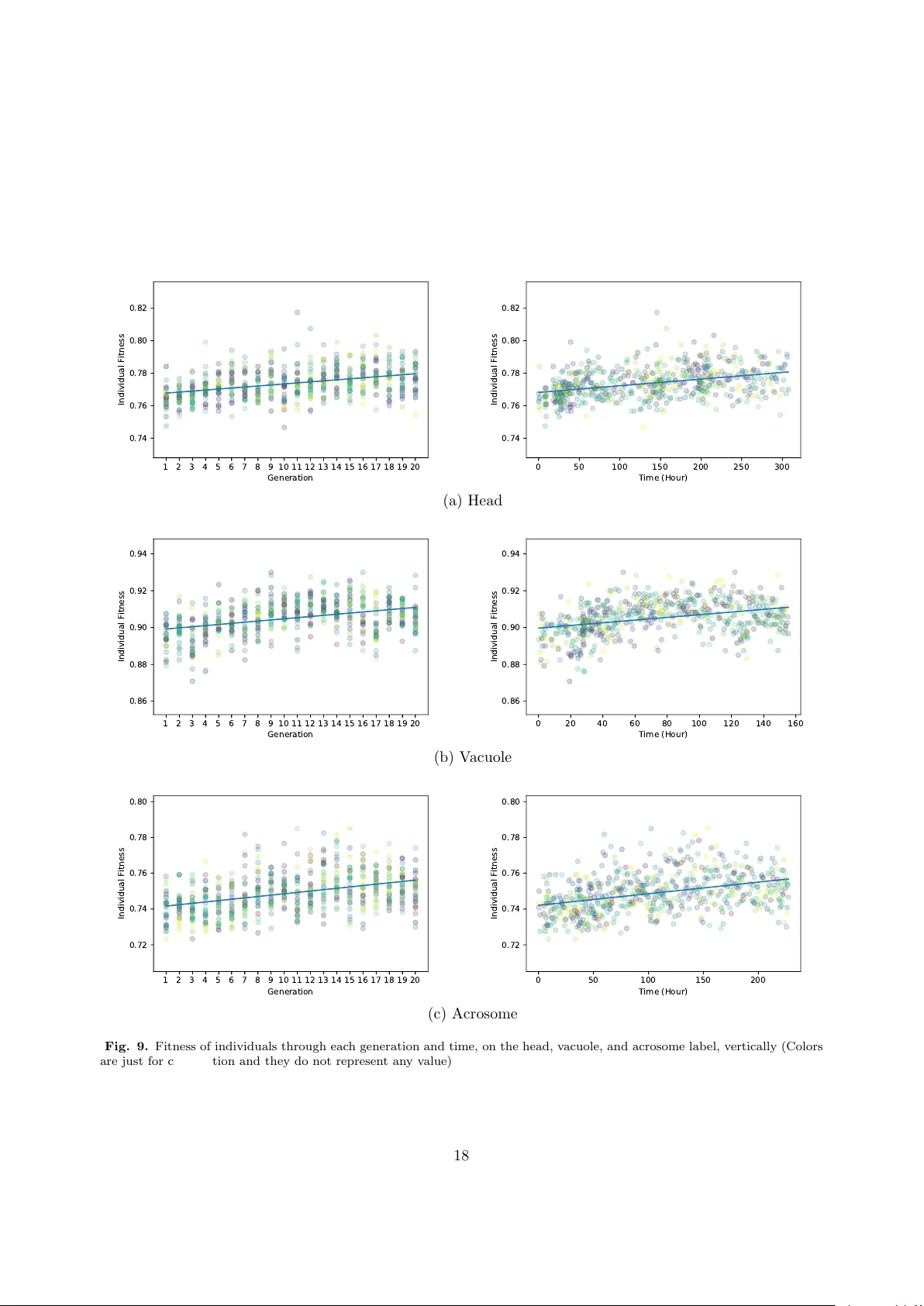
Genetic Neural Arc hitecture Searc h for automatic assessmen t of h uman sp erm images Erfan Miahi a , Sey edAb olghasem Mirroshandel a, ∗ , Alexis Nasr b a Dep artment of Computer Engine ering, University of Guilan, R asht, Ir an b L ab or atoir e d ´ Informatique et Systemes, Aix Marseil le Universit´ e, Marseil le, F r anc e Abstract Male infertilit y is a disease that aﬀects approximately 7% of men. Sp erm morphology analysis (SMA) is one of the main diagnosis metho ds for this problem. How ev er, manual SMA is an inexact, sub jective, non- repro ducible, and hard to teac h pro cess. Therefore, in this paper, we in tro duce a no v el automatic SMA tec hnique that is based on the neural arc hitecture searc h algorithm, named Genetic Neural Architecture Searc h (GeNAS). F or this purp ose, we used a collection of images termed MHSMA dataset, whic h con tains 1 , 540 sp erm images that hav e b een collected from 235 patients with infertilit y problems. In detail, GeNAS consists of a sp ecial genetic algorithm that acts as a meta-controller which explores the constrained search space of plain con volutional neural netw ork architectures. Ev ery individual of this genetic algorithm is a con volutional neural net work trained to predict morphological deformities in diﬀerent segments of human sp erm (head, v acuole, and acrosome). The ﬁtness of each individual is calculated b y a nov el proposed metho d, named GeNAS W eigh ting F actor (GeNAS-WF). This tec hnique is sp ecially designed to ev aluate the ﬁtness of neural net w orks which, during their learning process, v alidation accuracy highly ﬂuctuates. T o sp eed up the algorithm, a hashing metho d is practiced to sav e each trained neural architecture ﬁtness, so w e could reuse them during ﬁtness ev aluation. In terms of running time and computational p ow er, our prop osed architecture searc h metho d is far more eﬃcient than most of the other existing neural architecture searc h algorithms. Moreo ver, whereas most of the existing neural arc hitecture searc h algorithms are designed to w ork well with well-prepared b enchmark datasets, the ov erall paradigm of GeNAS is sp ecially designed to address the challenges of real-world datasets, particularly shortage of data and class imbalance. In our exp erimen ts, the b est neural arc hitecture found b y GeNAS has reached an accuracy of 91.66%, 77.33%, and 77.66% in the v acuole, head, and acrosome abnormality detection, resp ectiv ely . In comparison to other prop osed algorithms for MHSMA dataset, GeNAS achiev ed state-of-the-art results. Keywor ds: Human Sp erm Morphometry , Infertility , Genetic Algorithm, Deep Learning, Neural Arc hitecture Search. 1. In tro duction Appro ximately 15% of couples suﬀer from infertilit y , which is in 30 to 40% of the cases due to the male sp erm abnormalities ( Isidori et al. , 2005 ; Stouﬀs et al. , 2008 ). One of the k ey metho ds for male infertility diagnosis is sp erm morphology analysis (SMA), which consists of classifying sp erm head, v acuole, acrosome, and tail as normal or abnormal. Ho wev er, manual SMA suﬀers from sev eral ﬂaws. It is inexact, sub jective, non-repro ducible, and hard to teach pro cess. Therefore, in the past couple of years, several computer- based algorithms hav e b een prop osed to address these limitations and automate this process ( Ja v adi and Mirroshandel , 2019 ; Riordon et al. , 2019 ; Ghasemian et al. , 2015 ). ∗ Corresponding author. T el.: +98 13 33690274 (Ext. 3193); fax: +98 1333690271 Email addr esses: mhi.erfan1@gmail.com (Erfan Miahi), mirroshandel@guilan.ac.ir (SeyedAbolghasem Mirroshandel), alexis.nasr@univ-amu.fr (Alexis Nasr) Pr eprint submitte d to Elsevier Septemb er 18, 2020 Automating the SMA pro cess can b e seen as a computer vision classiﬁcation problem, whic h aims to classify sp erm’s head, v acuole, acrosome, and tail. Moreov er, in recent years, Con volutional Neural Net work (CNN) algorithms b ecame the state-of-the-art tec hnique in solving a lot of computer vision tasks ( V oulo dimos et al. , 2018 ), esp ecially in the area of image classiﬁcation ( Krizhevsky et al. , 2012a ; Szegedy et al. , 2016 ; Sugan uma et al. , 2017 ). As a result, these accomplishments mak e them a natural choice for addressing the SMA. Nevertheless, usually , a high price should be paid for using CNNs since they exhibit complex arc hitectures and need a large amoun t of exp ert kno wledge and computer resources to b e tuned. This is where Neural Architecture Searc h (NAS) algorithms come forw ard and attempt to o v ercome these c hallenges ( He et al. , 2019 ). These algorithms can b e describ ed as tec hniques that striv e to automate the pro cess of designing neural netw ork arc hitectures. They usually try to ac hiev e this purpose by adopting an eﬃcient searc h algorithm, such as Ev olutionary Algorithms ( Real et al. , 2017 ) or Reinforcement Learning ( Liu et al. , 2017 ), to searc h for optimal neural net work arc hitecture. Ho w ever, in the past few y ears, the studies on designing NAS algorithms ha ve confronted with several challenges. The early prop osed metho ds in the NAS domain were highly computationally exp ensiv e. In other w ords, they emplo y ed h undreds of GPU-hours to discov er a near-optimal neural arc hitecture. Nonetheless, more recen t algorithms attempted to tackle this challenge b y employing diﬀerent tec hniques, namely netw ork morphism ( Jin et al. , 2018 ), and predicting neural arc hitecture accuracy ( Baker et al. , 2017a ). How ever, just a small n umber of these techniques hav e succeeded to eﬀectiv ely reduce computational cost. F urthermore, many of the prop osed NAS techniques hav e b een ev aluated on b enchmark datasets, such as ImageNet ( Deng et al. , 2009 ) and CIF AR-10 ( Krizhevsky et al. , 2009 ). The main adv an tage of this is that the Machine Learning (ML) researchers can hav e an integrated testb ed to compare the p erformance of their algorithms. How ev er, the central disadv an tages of these could b e that prop osed algorithms could ov erﬁt to predeﬁned standard datasets. T o clarify , the problem with these datasets is that they do not represen t real- w orld datasets in industry , medicine, and econom y . Such datasets frequently are imbalanced and contain lo w-quality images with noisy lab els. They also suﬀer from the shortage of data, whereas standard datasets are w ell-prepared and do not exp erience these limitations. In this pap er, we adopted a dataset named Mo diﬁed Human Sp erm Morphology Analysis dataset (MSHMA), which contains the features often seen in practical datasets, esp ecially the ones in the ﬁeld of medicine ( Jav adi and Mirroshandel , 2019 ). In detail, the classes are highly imbalanced, particularly in the v acuole lab el; the n umber of images is not adequate; images are non-stained and noisy . The algorithm prop osed in this paper, termed Genetic Neural Architecture Searc h (GeNAS), can b e seen as a framework that employs a customized genetic algorithm to search for an optimal neural arc hitecture. In detail, the p opulation of this genetic algorithm comprises chromosomes, whic h each one represen ts a CNN architecture. A t ﬁrst, the population will b e initialized with random v alues and lengths. After ﬁtness calculation, sp ecial crossov er, mutation, and tournament selection op erators will be applied to the p opulation, and this step will b e repeated for a sp eciﬁc n umber of iterations. In this genetic algorithm, while crosso ver op eration explores the depth of neural arc hitectures by com bining the parents’ genomes, mutation explores the search space of genes’ v alues (e.g., ﬁlter-size and stride-size of CNN’s architectures). Moreo v er, the ﬁtness of each individual will b e computed using a sp ecial technique named GeNAS W eigh ting F actor (GeNAS-WF), which mainly designed to address the diﬃculties caused by sampling and data augmentation metho ds during training. After the genetic algorithm discov ers the optimal neural architecture, w e train the selected arc hitecture from scratch with diﬀerent settings. F or instance, w e increase the num b er of iterations and c hange our early stopping technique. Our exp erimen ts sho w that GeNAS can ﬁnd CNN architectures that are capable of reaching state-of- the-art accuracy , precision, and f 0 . 5 score on the head, acrosome, and v acuole classiﬁcation for MHSMA dataset ( Ja v adi and Mirroshandel , 2019 ), with few er parameters and lay ers, compared to hand-designed mo dels. Moreo ver, our prop osed method works automatically without an y human interv ention. The salien t features of GeNAS are: 1. A neural architecture enco ding which can explore an optimal constrained searc h space of CNN arc hitectures. 2. The ﬁrst and only NAS algorithm for addressing the sp erm abnormality detection problem 2 3. A crosso ver op eration for exploring the depth of neural architecture 4. A hashing metho d, for sa ving pairs of architecture and ﬁtness of eac h chromosome; and then, reusing them in the ﬁtness ev aluation stage to sp eed up the algorithm 5. The abilit y to ﬁnd the optimal architecture with just 1 Nvidia GPU in less than 10 days 6. A pruning algorithm during genot yp e to phenot yp e conv ersion to preven t phenotype (neural arc hitecture) from having negative output height and weigh t v alues. 7. A new ﬁtness computation metho d called GeNAS-WS which is sp ecially designed to work with noisy , lo w quality , and imbalanced datasets 8. A neural architecture search algorithm sp ecially designed to w ork with a challenging dataset which is highly imbalanced; that do es not ha v e enough training examples; which images are non-stained and noisy , which details are not clear and recorded with a low-magniﬁcation microscop e The pap er is structured as follo ws: in section 2 , previous neural arc hitecture searc h and sp erm assessment metho ds are introduced. Our prop osed algorithm is presented in details in section 3 . In the fourth section, MHSMA dataset, augmentation technique, our sampling metho d, and the results of our experiments b oth on Random Searc h and GeNAS are rep orted and compared to other results on this dataset. In the last section, the conclusion of our prop osed metho d and its results on MHSMA dataset are summarized. 2. Related W ork Existing studies in the NAS domain and automatic sp erm pro cessing are reviewed in this section. All the proposed NAS algorithms can b e broken down into three main elements: search space, p erformance estimation strategy , searc h strategy ( Elsk en et al. , 2018 ). W e will elaborate on these components in the follo wing subsection and conclude with a discussion on existing automated sp erm pro cessing techniques. 2.1. Neur al Ar chite ctur e Se ar ch Algorithms It is more than three decades that algorithms designed to discov er an optimal neural architecture exist. The ﬁrst of such algorithms employ ed evolutionary techniques, more precisely genetic algorithm, to search for the b est neural architecture and its w eights ( Miller et al. , 1989 ; Kitano , 1990 ; Schaﬀer et al. , 1992 ; Stanley and Miikkulainen , 2002 ). How ev er, the term NAS just b egan to show up in recent years. After the publication of Zoph and Le ( 2016 ), this term became p opular, and, since then, a lot of machine learning researc hers started to doing research in this ﬁeld. The main motiv ation of these researchers is to ov ercome the limitations which come with hand-designing neural netw ork architectures. In detail, such arc hitectures need a lot of time and exp ert knowledge to be designed. Moreov er, since the num b er of hyperparameters represen ting new arc hitectures has gro wn exponentially b y the adv ancement in the ﬁeld of deep learning, designing a goo d architecture b ecame a hard task ev en for expe rts. All these prop osed algorithms can be represen ted by three elements, which are discussed in the subsequent paragraphs. First, the search space can diﬀer dep ending on the algorithms. By search space, we mean the structure, n umber, and prop erties of neural net w ork la y ers and their connections that the algorithms plan to searc h through. F or instance, for computer vision tasks, while sev eral algorithms attempted to searc h through plain conv olutional neural net works ( Cai et al. , 2018 ), others tried to explore an expanded version of this searc h space, which can incorp orate skip-connections ( Real et al. , 2019 ). F urthermore, whereas some of these algorithms aimed to search for the whole architecture ( Baker et al. , 2017a ), others striv ed to searc h for a conv olutional blo c k (i.e., motifs) ( Zhong et al. , 2018 ; Zoph et al. , 2017 ). In more detail, in the latter v ersion, con volutional blo c ks are smaller components of the whole CNN, and they will b e rep eated in a sp ecial wa y to construct the whole architecture. Admitting all this, diﬀerent sizes of the search space hav e their own pros and cons. T o clarify , while c ho osing a large and complex searc h space can increase the no velt y of the disco vered architecture, it demands high computational p o wer and time. By considering this, to reduce the computational cost, the search space of GeNAS can only consist of comp onen ts of plain conv olutional neural netw orks. The second element is the search strategy . The search strategy can b e describ ed as the technique emplo yed to explore the search space in a w ay that can discov er the optimal or near-optimal neural 3 arc hitecture in terms of p erformance. In the past few years, a lot of tec hniques, such as Reinforcement Learning ( Liu et al. , 2017 ; Real et al. , 2019 ; Pham et al. , 2018 ; Cai et al. , 2018 ), Ba yesian Optimization ( Sno ek et al. , 2012 ; Shahriari et al. , 2016 ; Sno ek et al. , 2015 ; Kandasamy et al. , 2018 ), Ev olutionary Algorithm ( Real et al. , 2017 ; Xie and Y uille , 2017 ; Stanley and Miikkulainen , 2002 ; Mey er-Lee et al. , 2017 ; Miller et al. , 1989 ), and gradient-based metho ds ( Liu et al. , 2019 ), hav e b een used as the searc h strategy . Nonetheless, among all these approaches, ev olutionary algorithms and reinforcemen t learning are the p opular ones. The ﬁrst approach which p opularized the NAS domain employ ed a reinforcement learning algorithm ( Zoph and Le , 2016 ). Accuracy on the v alidation set was considered as the reward v alue of this technique. By using this reward and policy iteration algorithm as the main p olicy , a Recurrent Neural Netw ork (RNN) was trained to generate a v ariable-length string. This v ariable-length string describ es the structure and connectivity of neural architecture. As a result, while this metho d s ucceeded in impro ving the accuracy on datasets, such as CIF AR10, it w as highly computationally exp ensiv e (i.e., used 800 GPUs). Hence, it is not p ossible to use this technique in practice, esp ecially for small companies and individual researc hers. Another line of research applied an evolutionary algorithm ( Real et al. , 2017 ) for a classiﬁcation task on CIF AR10 and CIF AR100. This algorithm follows a simple evolutionary algorithm paradigm that ﬁrst initializes the population and then attempts to improv e this p opulation through crosso ver and m utation. A t last, whereas this algorithm achiev ed a competitive result compared to reinforcemen t learning and random search algorithms on CIF AR10, it e mplo yed a v ast amount of computational p o wer: 250 GPUs for 10 days. Nev ertheless, this challenge was addressed b y further researc h in this ﬁeld by prop osing eﬃcient p erformance estimation strategies. The third element of these algorithms is their p erformance estimation strategy . The p erformance estimation strategy can b e seen as the metho d used to estimate the p erformance of each arc hitecture. The computational b ottlenec k of most of the NAS algorithms lies in this elemen t. In other w ords, ev aluating eac h neural arc hitecture takes a lot of time compared to other comp onen ts of the proposed algorithms. Therefore, in recent years, most of the researc hers ha ve fo cused on this elemen t to reduce the computational cost and increase the eﬃciency of their algorithms. The simplest approach for estimating a neural netw ork’s p erformance is conv entional training and v alidation of neural netw orks. Ho wev er, since it is computationally exp ensive to this, recent algorithms attempted to abate this computational cost in v arious wa ys. T o illustrate, one of these metho ds tried to solv e this problem by using regression mo dels to predict the ﬁnal accuracy on the v alidation set of partially trained mo dels ( Baker et al. , 2017a ). Additionally , other proposed algorithms applied new tec hniques such as early stopping ( Baker et al. , 2017b ), training on a lo wer subset of the actual data ( Klein et al. , 2017 ), w eight inheritance (i.e., netw ork morphism) ( Elsken et al. , 2019 ), and weigh t sharing ( Pham et al. , 2018 ). How ever, while most of these metho ds eﬀectively reduce the computational cost, they usually underestimate the real p erformance of the disco v ered arc hitectures ( Elsken et al. , 2018 ). By considering this, we chose to reduce the computational cost in tw o wa ys. First, w e train eac h model for a limited but reasonable num b er of batc hes. Second, a hashing metho d is used to prev ent the rep etition of ev aluating the same neural arc hitecture. While most of the proposed algorithms were sp eciﬁcally inv ented to work with benchmark ed datasets, whic h are clean and well-prepared, there is a need for metho ds able to work with more noisy datasets that can b e found in v arious industries, such as medicine. Th us, in this pap er, our main concentration is on dev eloping a NAS algorithm that can work well with such datasets. In more detail, to address the problems of data shortage and data im balance, w e use a data aumen tation tec hnique and an o versampling metho d, resp ectiv ely . But, these techniques cause high ﬂuctuations in v alidation accuracy during training, whic h mak es it hard to measure when a mo del conv erges. T o cop e with these challenges, a sp ecial technique named GeNAS-WF as a p erformance estimation strategy is introduced in this pap er. 2.2. Automatic Sp erm Pr o c essing The automatic selection of sp erms has b een the ob jectiv e of many studies. In one of the studies, Ramos et al. ( 2004 ) combined computerized k aryometric image analysis (CKIA) system and DNA-speciﬁc stain 4 (F eulgen) for ev aluation of ICSI-selected epididymal sp erms. They hav e used a high magniﬁcation (1000 × ) microscop e. In another researc h, the fraction of b oar spermatozoa heads was measured and a pattern for this part w as trained ( Sanc hez et al. , 2006 ; S´ anc hez et al. , 2005 ). In this metho d, a deviation model is prop osed and calculated for each sp erm’s head. After that, an optimal v alue is obtained for the classiﬁcation of eac h sp erm. Then, sp erms tails, by utilizing morphological closing, w ere remov ed and the holes in the contours of the heads w ere ﬁlled. In the end, by applying Otsu’s metho d ( Otsu , 1979 ), the head of each sp erm is separated from the bac kground. In ( Vicen te-Fiel et al. , 2013 ), sp erm n uclear morphometric subp opulations of diﬀeren t sp ecies including goat, sheep, pig, and cattle were pro cessed using ImageJ ( Abr` amoﬀ et al. , 2004 ) and the results were used for m ultiv ariate cluster analyses. There is also another work in which the eﬀects of diﬀerent staining metho ds on the human sp erm head w ere reported ( Maree et al. , 2010 ). In their study , stained and fresh sperms w ere compared together. ImageJ also used in another metho d in order to assess ram sp erm morphology on the stained images ( Y´ aniz et al. , 2012 ). ( Zhang , 2017 ) has also prop osed a nov el metho d for animal sp erm morphology analysis. Diﬀerent algorithms such as activ e con tour mo del, K-means, thinning algorithm, and image momen t hav e b een utilized in this metho d. In another research, the Bay esian classiﬁer w as applied in order to extract diﬀerent parts of sp erm: acrosome, n ucleus, midpiece, and tail ( Bijar et al. , 2012 ). This segmen tation was done using Mark ov random ﬁeld mo del and the entrop y-based exp ectation-maximization algorithm on the stained human semen smear. The images w ere captured with a high-magniﬁcation (1000 × ) microscop e. Abbiram y and Shan thi ( 2010 ) prop osed a method for the classiﬁcation of sp erms in to normal and abnormal classes. Their metho d pro ceeds in four steps: 1) image prepro cessing: RGB to gra yscale con version and noise remov al by applying median ﬁlter; 2) sp erm detection and extraction using the Sob el edge detection algorithm; 3) segmen tation of each sperm; and 4) applying classiﬁcation to detect normal and abnormal sp erms. In another study , Combining learning v ector quantization (L VQ) and digital image pro cessing was used for the classiﬁcation of b oar sp erm acrosome ( Alegre et al. , 2008 ). The images were captured using a phase- con trast microscop e. This metho d w orks on stained images, and the experimental results ha ve shown a 6.8% error on the classiﬁcation task. A combination of histogram statistical analysis and clustering tec hniques is another metho d that has b een applied in sp erm detection and segmentation ( Chang et al. , 2014 ). In another research, principal comp onen t analysis (PCA) was also applied in order to extract features from sp erm images ( Li et al. , 2014 ). K-nearest neigh b ors (KNN) tec hnique was also used for the classiﬁcation of normal sp erms. There are also some metho ds that fo cus on microscopic videos for sp erms segmen tation and calculation of their motilities ( Haugen et al. , 2019 ; Boumaza et al. , 2018 ; Ilhan and Aydin , 2018 ). One of the successful methods for normal sp erm selection, whic h is able to w ork with fresh h uman sperms, is the algorithm of Ghasemian et al. ( 2015 ). This metho d w orks with images from a low-magniﬁcation microscop e (400 × and 600 × ), and the images are non-stained. One of the other adv antages of this metho d is its real-time pro cessing time. T o the best of our knowledge, there are only a few researc hers that applied deep learning for normal sp erms classiﬁcation. In one of these studies, the sp erms DNA in tegrity has been predicted from sp erm images using a deep CNN ( McCallum et al. , 2019 ). They ha ve trained CNN on a collection of appro ximately 1,000 sp erm cells of kno wn DNA qualit y , for prediction of DNA quality from brigh tﬁeld images. A pre-trained CCN architecture (i.e., V GG16) has been used in this study , and some additional lay ers w ere added after the last con volutional lay er. The achiev ed results were acceptable in terms of DNA integrit y prediction. In another deep learning metho d, sp erm images were classiﬁed in to the W orld Health Organization (WHO) shap e-based categories (i.e., Normal, T ap ered, Pyriform, Small, and Amorphous) ( Riordon et al. , 2019 ). The authors also used VGG16 in order to a void excessiv e neural net work computation. They hav e applied their method on tw o freely-a v ailable sp erm head datasets (HuSHeM ( Shak er , 2017 ) and SCIAN ( Chang et al. , 2017 )). The achiev ed results on sp erm classiﬁcation were sup erior to the other existing methods on these t wo datasets. How ever, this method cannot classify the diﬀeren t parts of eac h sp erm. 5 One of the most successful deep learning algorithms in sp erm classiﬁcation is the work of Ja v adi and Mirroshandel ( 2019 ). In their metho d, after applying data augmen tation tec hniques and a sampling metho d, a deep neural net work architecture w as designed and trained. This arc hitecture is able to detect morphological abnormalities in diﬀeren t parts of human sperm (i.e., acrosome, head, and v acuole). This algorithm w as trained and ev aluated on the MHSMA dataset, and the trained mo dels were highly accurate. It should b e noted that GeNAS is far more precise than this metho d, whic h is discussed in more detail in section 4.6 . 3. GeNAS In this section, we ﬁrst present the ov erall algorithm of GeNAS, then we fo cus on the chromosome structure, and the ﬁtness function. Finally , the primary customized op erations of selection, crossov er, and m utation are describ ed. 3.1. The over al l structur e of GeNAS The ov erall scheme of GeNAS is shown in Fig. 1 . The algorithm starts with initializing the p opulation b y generating n p n umber of chromosomes. The pro cess of generating eac h chromosome consists of t wo steps: ﬁrst, w e set the length of the chromosome b y sampling a random v alue from the feasible set; then, the v alue of eac h gene of the chromosome will be selected from a constrained search space, which is described in subsection 4.4 . Each c hromosome’s phenot yp e corresp onds to a CNN architecture that consists of conv olutional cells. Eac h conv olutional cell is made of a conv olution lay er, follow ed b y a max-p o oling lay er. During the genot yp e → phenotype translation pro cess, a pruning operation will take place if the genotype is not feasible, i.e., the output of the corresp onding con volutional neural architecture has negativ e heigh t and w eight v alues. Brieﬂy , the pruning op eration will cut some of the conv olutional cells in the chromosome’s head to mak e it feasible. Next, the phenot yp e of each individual is trained on n b n umber of mini-batches, and, after training on eac h mini-batc h, accuracy on the v alidation set is ev aluated and sa v ed. These accuracies will b e used, at a later stage, to compute the ﬁtness of the individual using the GeNAS-WF technique, which is explained in subsection 3.4 . Then parents selection is p erformed on the p opulation using tournamen t selection with a tournamen t size of n p 3 . At last, a special crossov er op eration with a probabilit y of p c , follow ed by a m utation op eration with a probabilit y of p m , is applied to the selected paren ts to produce a new p opulation. The crosso ver op eration can change the length of each child and helps to not only explore the search space of neural architectures with diﬀerent lengths but also exploit the best individuals in the p opulation. On the other hand, the m utation op eration will change genes’ v alue in genotype, so it is resp onsible for exploring the diﬀeren t num b er of ﬁlters and stride-size in the phenotype. These steps will b e rep eated for n i n umber of times. Then, the arc hitecture with the b est ﬁtness among all p opulations will b e chosen as the optimal neural architecture. A t the ﬁnal stage, the selected arc hitecture will b e trained on a higher n umber of mini-batches from scratc h. During this step, after training on each mini-batc h, the accuracy of the model on the v alidation set will b e ev aluated, and the mo del with a maximum of this accuracy will b e sa ved. At the last step, the sa ved mo del will b e assessed on the test set. The o verall structure of GeNAS is summarized as follow: 1. Randomly initialize eac h individual of the ﬁrst generation from the constrained search space. 2. Prune the genotype of each individual and translate it to the corresp onding phenotype, as shown in Fig. 2 . 3. T rain the individual for n b n umber of mini-batches, then use the GeNAS-WF metho d to compute its ﬁtness v alue. 4. If generation n i is reac hed, go to step 8. 5. P erform T ournament Selection with tournament size of n p 3 to select paren ts for crossov er op eration. 6. P erform the sp ecial crosso ver, introduced in subsection 3.6 , with the probability of p c . 6 7. P erform mutation, explained in subsection 3.7 , with probability of p m , then go to step 2. 8. Select the individual with the maximum ﬁtness v alue among all individuals of all p opulations as the optimal individual. 9. T rain the optimal individual for n 0 b n umber of mini-batc hes, and, during training, sa ve the mo del whic h has the maxim um accuracy on the v alidation set. 10. Ev aluate the optimal trained mo del on the test set and rep ort the test measures on the test set. Randomly initialize individuals Prune genotypes Convert them to phenotypes (1) (2) Train individuals Compute their ﬁtness by GeNAS-WF (3) NO YES Generation No. = n i (4) Select via tournament selection (5) Crossover (6) Mutate (7) Select best individual (8) Pick best checkpoint model (9) evaluate it on test set (10) Train it Fig. 1. Structure of GeNAS 3.2. Chr omosome Structur e The proposed c hromosome is a linear c hromosome with discrete genes’ v alues, which its genot yp e enco des the properties of the architecture of a CNN (phenot yp e). In this encoding sc heme, each chromosome encodes features of multiple con volutional cells. A conv olutional cell is comp osed of a conv olutional lay er following b y a max-p o oling lay er. Starting from the ﬁrst gene, every four distinct consecutiv e genes of a chromosome represen t the features of a conv olutional cell. Therefore, a c hromosome of length n c con tains n c 4 n umber of con volutional cells, and every chromosome’s length should b e a factor of four. In more detail, the ﬁrst three genes of a con volutional cell encode the num b er of ﬁlters, the ﬁlter-size (width and height of ﬁlters considered equal), and the stride-size of a con v olutional lay er. The fourth gene represents the stride-size (stride-size and max-po ol windo w size are considered equal) of a max-po oling la yer. F urthermore, while features of con volutional cells diﬀer depend on the c hromosome’s v alues, the last three lay ers of the phenotype are consisten t for all the c hromosomes. The structure of each genot yp e and its translation to phenotype is sho wn in Fig. 2 . Due to the deﬁnition of the chromosome, our prop osed linear chromosome can describ e an y plain con volutional neural arc hitecture. T o illustrate, if w e w ant to ha ve consecutive max-p ooling lay ers in our con volutional neural arc hitecture, w e can allow our searc h space to assign 0 v alue to the ﬁlter height and width size , whic h is equal to not ha ving a con volutional la yer. Additionally , when we w ant to ha ve consecutiv e conv olutional lay ers in our c on volutional neural architecture, we can allow our search space to assign v alue 1 to the stride-size (p o oling-size) of a max-p ooling lay er, which is equal to not having a max-p ooling lay er. Fig. 3 shows an example of genotype deco ding. 7 Genotype Phenotype Convolutional Layer Max Pooling Layer Convolutional Cell number of ﬁlters ﬁlter width and height stride size stride size Convolutional Layer Max Pooling Layer Convolutional Cell number of ﬁlters ﬁlter width and height stride size stride size Fully Connected Layer(1024 Neurons) Fully Connected Layer(1024 Neurons) Average Pooling Layer Fig. 2. T ranslation of the genotype of a chromosome to its phenotype in GeNAS 32 3 1 2 64 1 2 1 Genotype Phenotype Conv2D F:3x3 S:1 N:32 MaxPool P:2x2 S:2 Convolutional Cell number of ﬁlters ﬁlter width and height stride size stride size Conv2D F:1x1 S:2 N:64 Convolutional Cell number of ﬁlters ﬁlter width and height stride size Fully Connected Layer(1024 Neurons) Fully Connected Layer(1024 Neurons) Average Pooling Layer Fig. 3. A detailed example of genotype translation of a chromosome to its phenotype (Note that the last max-p o oling lay er is remov ed b ecause its stride-size is 1) 8 3.3. Pruning Before the ﬁtness ev aluation step, to make sure that the chromosome is feasible, a pruning pro cess will pro ceed. A chromosome considered infeasible when, b y stacking its corresp onding conv olutional cells, w e get a negative output from the constructed CNN. In the pro cess of genotype to phenotype translation, this happ ens b ecause often after we add a conv olutional or a max-p o oling lay er in each step to the phenotype, output dimensions of the phenotype will abate, according to equations 1 , 2 , 3 , and 4 . F or clariﬁcation, an example of the pruning process on a chromosome with four conv olutional cells is illustrated in the Fig. 4 . In this example, the padding size employ ed is zero for all conv olutional cells, so equations 3 and 4 are only used for calculating the output dimensions. In simple terms, when the output of a phenotype gets negativ e, w e cut enough conv olutional cells from its head, until we get p ositiv e output. Ho wev er, both for taking this pro cess in parallel with the genotype to phenotype translation into accoun t and accelerating it, we to ok another approac h in practice. In this approac h, b efore adding each conv olutional or max-p o oling lay er, we calculate the output dimensions of the whole netw ork, with the help of equations 1 , 2 , 3 , and 4 . Then, if we get a negative output, the translation pro cess will b e stopp ed, and the constructed CNN will b e sen t for ﬁtness ev aluation; otherwise, we add the la yer to the top of the phenotype and rep eat this pro cess. W new = ( W curr ent − F + 2 P ) /S + 1 (1) H new = ( H curr ent − F + 2 P ) /S + 1 (2) W new = ( W curr ent − F ) /S + 1 (3) H new = ( H curr ent − F ) /S + 1 (4) Where W new and H new are the new w eight and heigh t size, W curr ent and H curr ent are the current weigh t and height size, F is the ﬁlter-size, S is the stride-size, and P is the padding-size. These equations work b oth for calculating the dimension of conv olutional and max-p ooling lay ers’ output. The equations 1 and 2 take place when w e use padding, otherwise, the equations 3 and 4 are used. 3.4. Fitness Evaluation One of the indisp ensable comp onents of a genetic algorithm paradigm is formulating its ﬁtness function. In single-ob jectiv e optimization problems, a goo d ﬁtness function acts as an ob jectiv e function that maps a feasible solution to a scalar v alue, whic h is a summarization of its closeness to a set of desired aims. In the ﬁeld of mac hine learning, the common scalar v alue which has been used to ev aluate the p erformance of a neural netw ork is the accuracy of it on the v alidation set. Hence, since we w ant to discov er a high- p erformance mo del, and using the v alidation accuracy work ed well for the prior studies in the NAS domain, the ﬁtness v alue is obtained using the accuracy of the mo del on the v alidation set. Ho wev er, in comparison with previous studies, we used a diﬀerent technique to gain ﬁtness v alue from v alidation accuracy . The reason for prop osing this tec hnique is our experiments rev ealed that v alidation accuracy inordinately ﬂuctuates during the training phase. One example of these ﬂuctuations is shown in Fig. 6 . The cause of these ﬂuctuations lies in using a special sampling and data augmentation methods (explained in section 4 ) during the training phase, as sub-comp onents of GeNAS, to cop e with imbalanced data and shortage of data resp ectiv ely . W e termed this technique GeNAS-WF and, brieﬂy , it helps us to lev el oﬀ these ﬂuctuations. In this technique, to obtain this ﬁtness v alue for each solution, ﬁrst, we train it on n iter n umber of mini- batc hes. In the course of the training phase, after training on each mini-batch, the accuracy of the model on the v alidation set will b e accumulated in a vector named B . Just to clarify , the ﬁrst elemen t of vector B carries v alidation accuracy after training on the ﬁrst mini-batch, the second elemen t carries v alidation accuracy after training on the second mini-batc h, and it follows this pattern until the last element, which is n th iter elemen t. In the next step, we decide on a customized window, named W, which is a vector of size n w . Then, the cross-correlation b et w een B and W will b e calculated. This op eration will result in a smo other v ector G . F or illustration, the ﬁrst element of G is computed by calculating the weigh ted mean of one to n w 9 Pruning Output dimensions: 2x2x32 32 3 1 2 Genotype Phenotype Conv2D F:3x3 S:1 N:32 MaxPool P:2x2 S:2 Convolutional Cell Output dimensions: 1x1x256 256 1 1 2 Conv2D F:1x1 S:1 N:256 MaxPool P:2x2 S:2 Convolutional Cell Output dimensions: -1x-1x512 512 3 1 1 Conv2D F:3x3 S:1 N:512 Convolutional Cell Output dimensions: -1x-1x64 64 1 1 1 Conv2D F:1x1 S:1 N:64 Convolutional Cell 8x8x1 input image Output dimensions: 2x2x32 32 3 1 2 Genotype Phenotype Conv2D F:3x3 S:1 N:32 MaxPool P:2x2 S:2 Convolutional Cell Output dimensions: 1x1x256 256 1 1 2 Conv2D F:1x1 S:1 N:256 MaxPool P:2x2 S:2 Convolutional Cell 512 3 1 1 64 1 1 1 8x8x1 input image Before Pruning After Pruning Fig. 4. Pruning of a chromosome with four conv olutional cells elemen ts of vector B , the second elemen t is computed by calculating the weigh ted mean of tw o to n w + 1 elemen ts of vector B and so on, using W as the weigh ts. A t last, the maximum element of vector G will b e considered as the ﬁtness v alue of the mo del. The equations are as follows: G [ i ] = n w X u =0 W [ u ] ∗ B [ i + u ] f or i = 0 , 1 , 2 , ..., ( n iter − n w + 1) (5) f itness = n iter − n w +1 max i =0 ( G [ i ]) (6) In the equations ab ov e, characters in the square brac kets refer to the sp eciﬁc elemen t of their corresp onding v ectors. F or example, in the G[i] notation, the c haracter i indicates the i th elemen t of v ector G . Moreo ver, based on our experiments, we assigned the v alue of one to all elements of the vector W . Nev ertheless, it has the p otential to get other v alues for improving the p erformance on other datasets. An example of ﬁtness ev aluation, with a vector W same as the one we used in our exp erimen ts , is illustrated in Fig. 5 . 10 0.872 1 1 1 1 1 0.90 0.85 0.87 0.875 0.875 0.87 0.94 0.80 * * * * * 0.874 0.868 0.886 0.859 Window of size 5 (W) : V alidation accuracy for 10 mini-batches (B) : Results of cross-correlation (G) : Fitness = 0.886 0.81 0.82 0.848 Shifting Fig. 5. GeNAS-WF: An example of calculating the ﬁtness of a trained neural architecture 0 250 500 750 1000 1250 1500 1750 2000 Iteration 0.4 0.5 0.6 0.7 Accuracy on validation set smoothed on validation set Fig. 6. Fluctuations of a sample CNN accuracy on v alidation set through iterations on head lab el A t last, it is go o d to mention that to increase the GeNAS sp eed and remov e the redundant ev aluation of individuals, b efore the translation pro cess takes place, a hashing metho d is also proposed to chec k if the ﬁtness of the genot yp e has already b een computed, in which case, the previously computed ﬁtness is retriev ed; otherwise, the phenotype is pro duced, and its ﬁtness will b e computed. It is go o d to mention that the time-complexit y of retrieving the ﬁtness of the previously ev aluated chromosome is O(1). 3.5. Sele ction The paren t selection step is p erformed using tournament selection with a tournament size of n p 3 , where n p is the population size. In this selection metho d, n p 3 individuals are randomly c hosen from the p opulation, 11 among whic h the individual with maximum ﬁtness v alue is selected. T ournament selection has been chosen b ecause it allows controlling the selection pressure utilizing tournamen t size. T o clarify , as tournament size gets larger, the selection pressure gets higher and vice v ersa. T ournamen t size, therefore, will enable us to c hange the degree of exploration and exploitation. In more detail, b y c hanging the tournament size, w e can adapt our metho d to the a v ailable computational p o w er. T o illustrate, since a low amoun t of computational p o wer is considered for our exp eriments, we selected a high v alue of tournament size ( n p 3 ). In this w ay , we increased the degree of exploitation ov er exploration, so our metho d can discov er a near-optimal CNN architecture in a fair amount of time. 3.6. Cr ossover The crosso v er op eration com bines the genot yp es of tw o paren ts to form the genot yp e of an oﬀspring. The main con tribution of the crosso ver operation of our proposed algorithm is that it helps GeNAS to c hange the length of the chromosomes of the new population, i.e., changing the num b er of conv olutional cells. In our case, the crosso ver op eration combines genotypes of diﬀerent sizes and produce a genotype of yet another size. Crosso ver is applied on a pair of genotypes par ent 1 and par ent 2 selected through tournament selection. First, a num b er b etw een zero and one is randomly chosen. If it is less than threshold p c , then the crossov er op eration is p erformed on par ent 1 and parent 2 ; otherwise, parent 1 and parent 2 are added to the new generation after a m utation step. With having in mind that the num b er of genes in each generated c hild should b e a co eﬃcien t of four, the crosso ver is designed as follows. A crossov er point point 1 , which is an integer num b er b et ween 0 and length of the parent par ent 1 , is randomly c hosen. Next, a p oin t point 2 is computed for par ent 2 in accordance to equation 7 : point 2 = RandomI nteg er (0 , leng th ( par ent 2 ) 4 ) × 4+ ( point 1 mo d 4) (7) Where R andomInte ger function will generate a random in teger betw een 0 and leng th ( par ent 2 ) 4 from random uniform distribution. This equation will guaran tee that, in the further steps, crosso v er generates children whic h their length will b e a co eﬃcien t of four. Once point 1 and point 2 are deﬁned, the lengths of the t wo children can b e computed as follows: leng th ( chil d 1 ) = point 1 + ( leng th ( par ent 2 ) − point 2 ) (8) leng th ( chil d 2 ) = point 2 + ( leng th ( par ent 1 ) − point 1 ) (9) After computing the c hildren’s length, if the computed lengths exceed the maxim um and minimum of individuals’ length in constrained search space, point 2 will b e calculated again until b oth children’s length are v alid. When v alid v alues of point 1 and point 2 ha ve b een determined, each genome is cut in t wo with resp ect to its crossov er p oint. At the next step, the left part of par ent 1 is concatenated to the right part of par ent 2 to pro duce the ﬁrst child, and the left part of par ent 2 is concatenated to the right part of par ent 1 to generate the second c hild. An example of this op eration is shown in Fig. 7 . 12 64 2 Parent 1 1 3 1 16 20 40 point 1 64 34 Parent 2 2 3 point 2 64 34 2 3 64 34 2 1 64 2 1 1 64 34 2 3 64 34 2 3 64 34 2 3 1 16 20 40 Child 1 Child 2 Fig. 7. A crosso ver example which generates children with diﬀerent lengths. 3.7. Mutation The m utation op eration allo ws mo difying the n umber of ﬁlters, ﬁlter-size, and stride-size of con v olutional and max-p ooling lay ers for eac h individual. The mutation op eration will take place for each individual with m utation probability (i.e., p m ). Considering ev ery 4 consecutive genes represen ts a conv olutional cell, we grouped genes into four distinct groups, each one represents a distinct feature of a con v olutional cell: the num b er of ﬁlters, ﬁlter-size (i.e., ﬁlter width and height), con volutional stride-size, and p o oling stride-size. These groups are evident in Fig. 2 . Considering this, when the m utation tak es place for a sp eciﬁc chromosome, one of the genes from the selected c hromosome will be pic ked randomly . Later, the selected gene will be mutated diﬀerently dep ending on what group of genes it belongs to. If the c hosen gene belongs to the n umber of ﬁlters or ﬁlter-size group, a random element will b e selected from the resp ective feasible v alues asso ciated with the group of the selected gene, describ ed in section 4.4 . Otherwise, if the selected gene matc hes with the conv olutional or p o oling stride-size group, a γ v alue will b e calculated as follows. A t the ﬁrst step, the curren t stride-size will b e added to a ﬂoating-p oint v alue, which is randomly selected from a normal distribution with a mean of zero and v ariance of one. Subsequently , the minimum of obtained v alue in the previous step and resp ectiv e gene group maximum constrained v alue, describ ed in section 4.4 , will b e computed. After we obtained the γ v alue, for ac hieving the ﬁnal m utated stride-size, maximum of γ and minim um constrained v alue of the resp ectiv e gene group will b e calculated. The equations are as follo ws: γ = min( S tr ideS iz e + RandomN or mal () , M axC onstr aintS tr ideS iz e ) (10) M utatedS tr ideS iz e = max( γ , M inC onstr aintS tr ideS iz e ) (11) Where R andomNormal function will generate a random v alue with mean 0 and v ariance 1 from the normal distribution. MaxConstr aintStrideSize and MinConstr aintStrideSize are the maximum and minim um v alues p ermitted to use as stride size, resp ectively . 4. Exp erimen ts and Results In the following sections, the exp erimen tal part of our w ork is describ ed. First, the Mo diﬁed Human Sp erm Morphology Analysis dataset (MHSMA), which contains annotated images of human sp erm cells, is 13 T able 1 Data distribution of the MHSMA dataset Lab el # P ositive # Negativ e % p ositiv e % Negative Head 1 , 122 418 72 . 86 27 . 14 Acrosome 1 , 086 454 70 . 52 29 . 48 T ail and neck 1 , 471 69 95 . 52 4 . 48 V acuole 1 , 301 239 84 . 48 15 . 52 in tro duced. Next, the data augmentation tec hniques and an ov ersampling metho d, which w e hav e designed, is illustrated. Then, constrained search space along with the mo dules, which w e utilized in our search space, is explicated. At last, The details of GeNAS implementation and the results of GeNAS, random search, and previous b enc hmarks are discussed. 4.1. Dataset The MHSMA dataset ( Jav adi and Mirroshandel , 2019 ) is comp osed of 1,540 grayscale images of sp erms with both size of 64x64 and 128x128. This dataset is made from Human Sp erm Morphology Analysis dataset (HSMA-DS) ( Ghasemian et al. , 2015 ), in tro duced in 2015. All images hav e b een lab eled by sp ecialists with four binary labels: tail and neck, v acuole, head, and acrosome. The v alue of these labels can b e either normal (p ositiv e), or abnormal (negative). The distribution of negative and p ositiv e v alues with resp ect to the four lab els is giv en in T able 1 . This table reveals that the data is highly imbalanced in fav or of the p ositiv e class, whic h accounts for 72 . 86% up to 95 . 52% of the data, dep ending on the lab el. F urthermore, W e ha ve used the split of the data prop osed by ( Ja v adi and Mirroshandel , 2019 ) in three subsets: training, v alidation, and test, which contain 1000, 240, and 300 images, resp ectively . Fig. 8. Sample images from MHSMA dataset. As it is visibile, the images are non-stained and low-resolution. 4.2. Data augmentation In this task, eac h trained con volutional neural netw ork should map an input sp erm image to a 1-bit lab el (i.e., abnormal and normal). Most generated neural architectures by GeNAS hav e parameters in the order of millions. So, as the num b er of the neural architecture parameters increases, more training examples are needed to prop erly tune the parameters. But, the MHSMA dataset has only 1000 training examples, and the act of collecting more human sp erm images is extremely costly and arduous. Moreo ver, to the b est of our kno wledge, MHSMA is one of the largest datasets in the ﬁeld of sperm morphology analysis. As a result, F or solving the problem of training examples shortage, a data augmen tation technique is adopted to prev ent ov erﬁtting and virtually increasing training set size. 14 In this technique, before feeding each training example (sp erm image) to the mo del, a 64x64-pixel crop will b e extracted from eac h 128x128-pixel image. After crop extraction step, w e apply random mo diﬁcations to eac h training example which they are as follows: • Flipping: Ev ery image was ﬂipp ed vertically and horizontally with the probability of 0.5. • Rotating: The cropp ed area of every image was rotated by θ degrees, where θ is randomly selected regarding the uniform distribution of [0 , 360). • Shifting: The crop region w as shifted along the vertical and horizontal axis by y and x pixels, where y and x w ere randomly chosen regarding the uniform distribution of [ − 5 , 5]. • Scaling: Pixel v alues of eac h image was multiplied by e β , where β is randomly c hosen regarding the uniform distribution of [ − log (1 . 25) , l og (1 . 25)]. The output of these random mo diﬁcations on one training example will b e a 64x64 gray-scale image. Ultimately , the image will b e normalized by subtracting it from its mean and dividing the result b y 255, as sho wn in equation 12 (x is a single sp erm image): nor mal ( x ) = x − mean ( x ) 255 (12) It is go od to mention that our augmentation settings are the same as the ones used in ( Jav adi and Mirroshandel , 2019 ) w ork. 4.3. Sampling As shown in T able 1 , the MHSMA dataset is highly imbalanced. Hence, a sp ecial o versampling metho d, prop osed b y Ja v adi and Mirroshandel ( 2019 ), is utilized to address this challenge. The main goal of this o versampling metho d is generating balanced mini-batches from an imbalanced dataset like the MHSMA. In this o versampling method, negative and positive samples will b e divided in to tw o distinct sh uﬄed lists. The pro cess of adding one sample to each mini-batch is as follows. First, we choose one of the lists by 0 . 5 probability . Next, the ﬁrst sample at the top of the chosen list will b e selected, and it will b e added to the mini-batch. At last, the selected sample will b e mov ed to the end of the chosen list. F or generating each mini-batc h, this pro cess will b e rep eated until the mini-batc h fulﬁlled. Moreov er, after all of the samples in a list is used, the list will b e shuﬄed. By using this approach, most likely , classes in every mini-batch will b e balanced. 4.4. GeNAS Se ar ch Sp ac e Our search space contains plain conv olutional architectures max-p o oling and conv olutional lay ers, with Scaled Exponential Linear Units (SELUs) ( Klambauer et al. , 2017 ) as non-linearities. SELU is emplo yed b ecause it will keep the neuron activ ations close to unit v ariance and zero mean, so it will let us increase the depth of a con volutional architecture without considering v anishing and explo ding gradients problem. As our search space gets bigger, ﬁnding the optimal con volutional architecture will b e harder and needs more time and computational p ow er. So, with inspiration from previous popular conv olutional arc hitectures ( Lecun et al. , 1998 ; Krizhevsky et al. , 2012b ; Zeiler and F ergus , 2013 ) a constrained searc h space is designed. In this constrained search space, for each conv olutional lay er, the meta-controller (Genetic Algorithm) should select a ﬁlter-size in { 1, 3, 5, 7, 11 } , num b er of ﬁlters in { 4, 8, 16, 32, 64, 128, 256 } , and con volutional cell stride-size in range of [1, 2]. Additionally , for each max-po oling la yer, it should select stride-size in range of [1, 2]. In addition to these constraints, 2 up to 50 num b er of conv olutional cells (i.e., an individual with a minim um length of 8 up to 200 genomes) is p ermitted. It should b e noted that the same constrained searc h space is emplo yed to discov er a sub-optimal neural arc hitecture for each lab el. 15 4.5. GeNAS Implementation Details In our exp erimen ts, the initial population consists of 30 individuals, which each of them is generated with b oth random length and random genes’ v alue from the constrained search space. Moreov er, the num b er of generations (iterations) has set to 20, and, in eac h of these generations, the p opulation size will be equal to the initial p opulation size. Exp erimen tal details of genotype to phenotype transformation are as follows. After the input lay er and con volutional cells created, one av erage-p ooling lay er with a stride-size of 2 follo wed by tw o fully connected la yers with 1024 neurons will b e added to the end of the phenotype. Then, one neuron with sigmoid as its activ ation function (output lay er) will b e app ended to the top of the last added fully connected lay er. It should b e considered that the SELU is adopted as the activ ation function of the tw o fully connected lay ers. An example of these conﬁgurations is depicted in Fig. 3 . Moreov er, the SELU activ ation function is an Exp onen tial Linear Unit (ELU) activ ation function which is scaled so that the v ariance and mean of the inputs will b e main tained in their original state b et ween t w o consecutiv e la yers. The equations for both SELU and ELU are as follo ws: selu ( x ) = scal e × elu ( x, α ) (13) elu ( x, α ) = ( x, if x ≥ 0 α ( e x − 1) , otherwise (14) After the whole CNN arc hitecture of the resp ectiv e genotype is created, its w eights will be initialized using the LeCun normal initializer ( LeCun et al. , 2012 ), and its biases will b e initialized to zero. In the LeCun normal initializer, the samples will b e drawn from a truncated normal distribution with a standard deviation of r 1 n input and zero as the center, where n input is the n um b er of inputs to the weigh t matrix. A t the next step, it will be trained for 2000 mini-batches. F or optimization, ADAM optimizer ( Kingma and Ba , 2014 )- with a constan t learning-rate of 10 − 4 , exp onen tial decay rates for the moment estimates of β 2 = 0 . 999, and β 1 = 0 . 9- is employ ed. In detail, ADAM is an algorithm for ﬁrst-order gradien t-based optimization of sto chastic ob jective functions, rooted in adaptive estimates of low er-order momen ts. F or loss function, binary cross-en tropy is applied, and each mini-batch contains 32 training images. After w e train the CNN, the ﬁtness of it will b e calculated by the GeNAS-WF metho d. F or this metho d, we c hose a window with a size of 5 and v alue of [1 , 1 , 1 , 1 , 1], same as the windo w shown in the Fig. 5 . Concerning the tournament selection, a tournament-size of 10 is chosen that, in a later stage, will select 30 fav orable paren ts for the next generation. Regarding the crossov er and mutation op erations, after exp erimen ting with v arious crosso ver and m utation probabilities for eac h task, the b est ones, we came up to, were 0.7 ( p c ) and 0.3 ( p m ) resp ectiv ely . Moreov er, the same algorithm, with the same settings, is used to do all three tasks which are obtaining the optimal conv olutional architectures that can predict abnormalit y in the sp erm head, v acuole, and acrosome on the MHSMA dataset. Our exp eriments w ere done, using Keras ( Chollet et al. , 2015 ) with T ensorﬂow ( Abadi et al. , 2016 ) bac kend on one Nvidia GPU. 4.6. R esults Before discussing our results, w e wan t to address the measurements employ ed to ev aluate the mo dels found by GeNAS. In our experiments, w e to ok accuracy , recall, precision, and f 0 . 5 score into accoun t as metrics for our ev aluations. The formulations of these ev aluation metrics are sho wn in equation 15 - 18 , where FN, FP , TN, and TP indicate false negativ e (i.e., regular sp erms predicted wrongly), false p ositive (i.e., irregular sp erms predicted wrongly), true negative (i.e., irregular sp erms predicted correctly), and true p ositive (i.e., regular sperms predicted correctly) resp ectively . It should b e mentioned that in our exp erimen ts, for t wo reasons, we considered the v alue of β in equation 18 equal to 0 . 5 (i.e., f 0 . 5 ). First, previous pap ers practiced this same metric for their ev aluations. Second, f 0 . 5 measure is more dep endent 16 on the precision rather than recall. Hence, since, in sp erm morphology , precision is more imp ortan t than recall, this v alue is a go o d metric to b e used. Accuracy = T P + T N T P + T N + F P + F N (15) Precision = T P T P + F P (16) Recall = T P T P + F N (17) F β score = (1 + β 2 ) × Precision × Recall β 2 × Precision + Recall (18) W e hav e employ ed GeNAS to discov er the b est architectures, which can predict abnormality in the sp erm head, v acuole, and acrosome indep enden tly . After the meta-controller trained and ev aluated on 600 arc hitectures (i.e., 30 individuals in 20 generations), we extracted the arc hitecture with the b est ﬁtness. The searc hing pro cess for each lab el shown in the Fig. 9 . According to this ﬁgure, for eac h lab el, the o verall ﬁtness has gradually increased during the ev olution pro cess. F or clariﬁcation, the linear regressions of all the points in each chart in Fig. 9 are calculated and shown. With resp ect to these c harts, GeNAS to ok appro ximately 310, 162, and 240 hours on just one GPU to run for the head, v acuole, and acrosome respectively . Therefore, considering that designing these architectures will take plen t y of time for a human expert, it is less time consuming and less arduous to use GeNAS instead of hand designing these architectures. After the b est chromosome extracted, it has b een trained for 20,000 mini-batches. The v alidation accuracies, for each lab el ov er iterations of training, are illustrated in Fig. 10 . It should b e noted that, in this ﬁgure, curves ha ve b een smo othed using a technique termed Simple Exp onen tial Smo othing ( Gardner Jr , 1985 ). The b est disco vered arc hitectures are shown in Fig. 11 , Fig. 12 , and Fig. 13 . F or the head lab el, illustrated in Fig. 11 , the neural architecture found by GeNAS consists of 12 conv olutional and three max-p ooling lay ers. 17 1 2 3 4 5 6 7 8 9 10 11 12 13 14 15 16 17 18 19 20 Generation 0.74 0.76 0.78 0.80 0.82 Individual Fitness 0 50 100 150 200 250 300 Time (Hour) 0.74 0.76 0.78 0.80 0.82 Individual Fitness (a) Head 1 2 3 4 5 6 7 8 9 10 11 12 13 14 15 16 17 18 19 20 Generation 0.86 0.88 0.90 0.92 0.94 Individual Fitness 0 20 40 60 80 100 120 140 160 Time (Hour) 0.86 0.88 0.90 0.92 0.94 Individual Fitness (b) V acuole 1 2 3 4 5 6 7 8 9 10 11 12 13 14 15 16 17 18 19 20 Generation 0.72 0.74 0.76 0.78 0.80 Individual Fitness 0 50 100 150 200 Time (Hour) 0.72 0.74 0.76 0.78 0.80 Individual Fitness (c) Acrosome Fig. 9. Fitness of individuals through each generation and time, on the head, v acuole, and acrosome lab el, vertically (Colors are just for clariﬁcation and they do not represent any v alue) 18 0 2500 5000 7500 10000 12500 15000 17500 20000 Iteration 0.60 0.65 0.70 0.75 0.80 0.85 Accuracy validation set training set (a) Acrosome 0 2500 5000 7500 10000 12500 15000 17500 20000 Iteration 0.60 0.65 0.70 0.75 0.80 Accuracy validation set training set (b) Head 0 2500 5000 7500 10000 12500 15000 17500 20000 Iteration 0.78 0.80 0.82 0.84 0.86 0.88 0.90 0.92 0.94 Accuracy validation set training set (c) V acuole Fig. 10. T raining and v alidation accuracy ov er iterations of training 19 Conv2D F:7x7 S:1 N:64 Conv2D F:7x7 S:1 N:64 Conv2D F:7x7 S:1 N:128 Conv2D F:5x5 S:1 N:8 Conv2D F:1x1 S:1 N:128 Conv2D F:1 1x1 1 S:1 N:8 Conv2D F:7x7 S:1 N:16 Conv2D F:7x7 S:1 N:16 Conv2D F:7x7 S:1 N:32 Image Conv2D F:7x7 S:2 N:4 AveragePool P:2x2 S:2 FullyConnected N:1024 FullyConnected N:1024 Prediction Sigmoid Activation MaxPool P:2x2 S:2 Conv2D F:7x7 S:1 N:16 MaxPool P:2x2 S:2 Conv2D F:1x1 S:1 N:128 MaxPool P:2x2 S:2 Fig. 11. Arc hitecture of b est mo del for sp erm head lab el F or the acrosome lab el, represented in Fig. 12 , the neural architecture discov ered by GeNAS includes 18 con volutional and ﬁve max-p o oling la yers. 20 Conv2D F:5x5 S:1 N:128 Conv2D F:5x5 S:1 N:128 Conv2D F:5x5 S:1 N:16 Conv2D F:1x1 S:1 N:32 Conv2D F:5x5 S:1 N:32 Conv2D F:1x1 S:1 N:256 Conv2D F:1x1 S:1 N:64 Conv2D F:7x7 S:1 N:16 Image Conv2D F:5x5 S:1 N:256 AveragePool P:2x2 S:2 FullyConnected N:1024 FullyConnected N:1024 Prediction Sigmoid Activation MaxPool P:2x2 S:2 Conv2D F:3x3 S:1 N:16 Conv2D F:1 1x1 1 S:1 N:8 MaxPool P:2x2 S:2 Conv2D F:5x5 S:1 N:8 Conv2D F:7x7 S:1 N:256 MaxPool P:2x2 S:2 Conv2D F:3x3 S:1 N:8 Conv2D F:5x5 S:1 N:128 Conv2D F:7x7 S:1 N:64 MaxPool P:2x2 S:2 Conv2D F:7x7 S:1 N:64 Conv2D F:3x3 S:1 N:128 MaxPool P:2x2 S:2 Fig. 12. Arc hitecture of b est mo del for sp erm acrosome lab el F or the v acuole lab el, shown in Fig. 13 , the neural architecture ascertained b y GeNAS is formed of 10 con volutional and ﬁve max-p o oling la yers. 21 Conv2D F:5x5 S:1 N:64 Conv2D F:5x5 S:1 N:64 Conv2D F:5x5 S:1 N:256 Conv2D F:1x1 S:1 N:8 Conv2D F:5x5 S:1 N:8 Conv2D F:5x5 S:1 N:256 Image Conv2D F:5x5 S:1 N:128 AveragePool P:2x2 S:2 FullyConnected N:1024 FullyConnected N:1024 Prediction Sigmoid Activation Conv2D F:3x3 S:1 N:16 MaxPool P:2x2 S:2 Conv2D F:7x7 S:1 N:4 MaxPool P:2x2 S:2 MaxPool P:2x2 S:2 Conv2D F:7x7 S:1 N:32 MaxPool P:2x2 S:2 MaxPool P:2x2 S:2 Fig. 13. Arc hitecture of b est mo del for sp erm v acuole lab el A t last, the discov ered neural architectures were ev aluated on the test set. The confusion matrix w as generated and represen ted in T able 2 . T able 2 Confusion matrix for ev aluation of best mo dels found by GeNAS on test set, for each lab el Lab el Actual class Predicted class Normal Abnormal Acrosome 178 true p ositiv es 32 false p ositives Normal 35 false negativ es 55 true negativ es Abnormal Head 185 true p ositiv es 34 false p ositives Normal 34 false negativ es 47 true negativ es Abnormal V acuole 249 true p ositiv es 12 false p ositives Normal 13 false negativ es 26 true negativ es Abnormal T o the b est of our knowledge, the only pap er designed a con volutional neural netw ork for the MHSMA 22 dataset is ( Jav adi and Mirroshandel , 2019 ) paper. As sho wn in T able 3 , in this pap er, the same neural arc hitecture comp osed of tw o max-p ooling and 24 conv olutional lay ers follow ed by one a verage-po oling lay er and tw o fully-connected lay ers is prop osed for predicting the abnormality on each lab el. On the other hand, GeNAS identiﬁed distinct neural architectures for each lab el. Additionally , in comparison with Jav adi and Mirroshandel ( 2019 ) pap er, the b est architecture found b y GeNAS consists of less than half the num b er of con volutional lay ers and three more max-p o oling lay ers for the v acuole lab el; half the num b er of conv olutional la yers and one more max-po oling la y ers for the head lab el; and 6 less n umber of conv olutional lay ers and three more max-p o oling la yers for the acrosome lab el. At last, it is go od to mention that the same n umber of av erage-p ooling and fully-connected lay ers with the same num b er of neurons are used in all architectures. The results of this metho d are shown as “Ja v adi et al.” in the T able 4 . T able 3 Comparison of num b er of diﬀerent lay ers in GeNAS and Jav adi et al. paper ( Jav adi and Mirroshandel , 2019 ) Lab el metho d conv olutional max-p o oling fully-connected a verage-po oling total Acrosome GeNAS 18 5 2 1 26 Ja v adi et al. 24 2 2 1 29 Head GeNAS 12 3 2 1 18 Ja v adi et al. 24 2 2 1 29 V acuole GeNAS 10 5 2 1 18 Ja v adi et al. 24 2 2 1 29 Another exp eriment that we conducted was ab out running a random search to ﬁnd the b est arc hitectures whic h can predict abnormalit y in the sp erm head, v acuole, and acrosome. In the beginning, random searc h trained 600 distinct CNN architectures (similar to our prop osed metho d), randomly generated from constrained search space. Then, every trained architecture was ev aluated on the v alidation set, and the architecture with the highest v alidation accuracy selected. In the next step, the selected arc hitecture w as trained for 20,000 mini-batches (i.e., the same as GeNAS). After training on each mini-batc h, accuracy on the v alidation set computed and the c hec kp oin t with the highest v alidation accuracy sav ed. Finally , the trained mo del ev aluated on the test set and test accuracy , precision, recall, and f 0 . 5 score calculated. The results are shown in the T able 4 . Another pap er prop osed an image pro cessing based algorithm to predict abnormality on the h uman sp erm morphology analysis dataset (HSMA-DS), whic h is the dataset that MHSMA based on Ghasemian et al. ( 2015 ). Their algorithm has b een assessed on t wo of the labels: head and v acuole. The results of this metho d are shown as “Ghasemian et al.” in the T able 4 . T able 4 Comparison of results of b est mo dels found by GeNAS with other prop osed metho ds on test set (all v alues are in p ercen t except parameters) Lab el Metho d Accuracy Precision Recall F 0 . 5 score P ar ameter s Acrosome GeNAS 77.66 84.76 83.56 84.52 5,756,553 Random Searc h 69.66 74.5 86.8 76.67 1,185,209 Ja v adi et al. 76.67 85.93 80.28 84.74 5,637,649 Ghasemian et al. N/A N/A N/A N/A N/A GeNAS 77.33 84.47 84.47 84.47 1,908,261 Random Searc h 76.00 80.49 88.58 81.98 3,032,401 Ja v adi et al. 77.00 83.48 85.39 83.86 5,637,649 Head Ghasemian et al. 61.00 76.71 71.79 75.68 N/A GeNAS 91.66 95.40 95.03 95.32 2,211,461 Random Searc h 89.00 94.20 93.12 93.98 4,715,861 Ja v adi et al. 91.33 94.36 95.80 94.65 5,637,649 V acuole Ghasemian et al. 80.33 83.21 93.56 85.09 N/A 23 Ev entually , as shown in T able 4 , GeNAS disco vered con v olutional architectures with higher accuracy , precision, and f 0 . 5 on the test set for all three lab els, except the precision on acrosome. It also achiev ed b etter recall on the head lab el in comparison with random search and previous metho ds. Additionally , the discov ered mo dels by GeNAS for b oth the v acuole and head lab els hav e extremely fewer parameters in comparison with other methods, with the exception of Random search on the acrosome lab el. Ho w ever, the accuracy , precision, and f 0 . 5 score of the random searc h on this lab el can not comp ete with the v alue of these metrics for GeNAS. Lastly , it should b e considered that critical measures for this dataset are precision and accuracy . Accordingly , the more inferior v alue of recall on the acrosome and v acuole lab els will not harm the p erformance of our mo dels. Based on our exp eriments, the inference-time of all discov ered mo dels is less than 1 second, whic h is a prop er time for treatment purp oses. 4.7. Visual explanation T o make sure that the b est neural architectures found b y GeNAS pay attention to the relev ant parts of sp erm images for making predictions, we applied a visual explanation technique named Gradient-w eigh ted Class Activ ation Mapping (Grad-CAM) ( Kotik alapudi et al. , 2017 ; Selv ara ju et al. , 2016 ). This visualization tec hnique will employ class-sp eciﬁc gradien t information to generate a heatmap, which emphasizes the areas of the input image that are essen tial for classiﬁcation. This visual explanation will provide us with a b etter understanding of the function of our neural architectures. Visual explanations of mo dels discov ered by GeNAS are shown in Fig. 14 for 3 diﬀeren t sample images which were c lassiﬁed accurately . These visual explanations illustrate the discov ered mo dels ha ve certainly learned to consider the sperm image areas whic h are, in fact, imp ortant for the sp erm abnormality prediction task. F or clariﬁcation, if we compare the visual explanation shown in Fig. 14 with the diagram of a sp erm represented in Fig. 15 , we will b e noticed that our models pa y atten tion to the exact relev ant fragments of sperm image for each classiﬁcation task, i.e., parts of the head, acrosome, and v acuole of sp erms. (a) Head (b) V acuole (c) Acrosome Fig. 14. Grad-CAM visual explanations for each lab el (warmer colors illustrate more attention) 4.8. Discussion Not only w e ac hiev ed better test accuracy on three distinct labels of the MHSMA dataset but also reached an outstanding precision in comparison with prior prop osed mo dels by Ghasemian et al. ( 2015 ), Jav adi and Mirroshandel ( 2019 ), and Random Search. F urthermore, GeNAS found neural architectures with extremely few er parameters for v acuole and head lab els and appro ximately the same n umber of parameters on acrosome compared with the neural arc hitecture introduced in ( Jav adi and Mirroshandel , 2019 ) pap er. In contrast, disco vered mo dels hav e reached less recall v alue on the head and v acuole lab els compared with previous pap ers. But, it should b e considered that precision and test accuracy are remark ably more imp ortan t than recall on this dataset. 24 M id p ie c e H e a d A c r os om e V a c uole s T a il Fig. 15. Diagram of distinct parts of a human sp erm cell ( Jav adi and Mirroshandel , 2019 ). In the domain of sp erm morphology analysis, esp ecially in abnormality detection of diﬀeren t segments of sp erms, precision and accuracy are more signiﬁcant compared with other measurements b ecause by ﬁnding ev en one normal sp erm and using it in intracytoplasmic sp erm injection (ISCI) pro cess, one can say that treatmen t pro cess can b e completed successfully . Hence, since discov ered models gained exceptional precision and accuracy v alues on all three lab els, they can b e used to take sp erm morphology analysis a step further to real-world applications in the ISCI pro cess. F urthermore, our discov ered mo dels can b e utilized to work with cheaper medical to ols lik e microscop es which are able to only tak e low-qualit y images mainly b ecause our tec hnique is sp ecially designed to w ork with such images. Therefore, they can classify sp erms ev en in p oor areas that do not hav e high-qualit y to ols. Lastly , it is goo d to consider im balanced datasets are mainly found in the medical industry ( Estev a et al. , 2019 ), and GeNAS can be used to tac kle many of these problems in this ﬁeld in the future. GeNAS can be employ ed to tac kle an y binary and m ulti-class image classiﬁcation problems. It, nev ertheless, w ould be better to customize the constrained searc h space of GeNAS concerning computational pow er and dataset characteristics. In detail, for datasets with high-resolution images, it is recommended to expand the range of stride-size b oth for conv olutional and max-po oling la yers. On the other hand, for lo w-resolution images, the opp osite is the case. Moreo ver, dep ending on the av ailable computational p ow er, we can change the tournamen t size. T o clarify , if we hav e a high amoun t of computational p ow er, w e can decrease the tournamen t size. In this wa y , the degree of exploration will be increased and more areas of searc h space will b e explored. As a result, b etter arc hitectures can b e disco vered. In contrast, for the lo w amount of computational p o w er, it is go o d to abate the tournament size. F urthermore, due to our experiments, we hypothesis that increasing the num b er of generations will result in disco vering b etter architectures. Hence, with more computational pow er and time, b etter neural arc hitectures can b e obtained. At last, it should b e noted that, for multi-class image classiﬁcation problems, the softmax function should b e used instead of the sigmoid function in the last lay er. F or future works in this area, multi-ob jectiv e neural architecture search algorithms can b e introduced to maximize both accuracy and precision on the v alidation set, and, for applications in the real-w orld problems, whic h should b e done in real-time, inference time should b e one of the ob jectiv es. F urthermore, new modules can be added to the search space, suc h as skip-connections, or more eﬃcient searc h spaces can be designed to tac kle problems in the real w orld. Additionally , further w ork can b e done to automate the other comp onen ts of the image classiﬁcation pro cess, such as data cleaning and mo del selection, on imbalanced datasets. 5. Conclusions W e prop osed a p ow erful and eﬃcien t algorithm termed Genetic Neural Architecture Searc h (GeNAS) for sperm abnormality detection. In this work, a nov el ﬁtness (ob jectiv e) function named GeNAS w eighting factor (GeNAS-WF) introduced to ev aluate the appropriateness of each generated architecture b y GeNAS. This ob jective function tends to work well with all neural architecture search algorithms designed to work with datasets that are im balanced and suﬀer from data shortage. F urthermore, the GeNAS algorithm can b e employ ed to discov er the b est con volutional neural netw ork architecture capable 25 of ultimately tac kling an y image classiﬁcation problem, speciﬁcally on noisy , lo w quality , and imbalanced datasets, which primarily app ear in real-w orld scenarios. Empirically , we prov ed that GeNAS can ascertain b etter state-of-the-art architectures- in terms of accuracy , precision, and f 0 . 5 measure- compared to previously prop osed metho ds, such as hand-designed CNN architectures, image pro cessing approac hes, and random search, with less amoun t of computational p o w er and h uman eﬀort on all three acrosome, head, and v acuole lab els of MHSMA dataset. Additionally , The arc hitectures discov ered by GeNAS ha ve exceptionally few er parameters on the head and v acuole labels . Finally , concerning the lack of NAS researc h to address the challenges of real-world datasets, we recommend that further researc h should b e done in this area of researc h. References References Abadi, M., Barham, P ., Chen, J., Chen, Z., Davis, A., Dean, J., Devin, M., Ghemaw at, S., Irving, G., Isard, M., et al., 2016. T ensorﬂow: a system for large-scale machine learning, in: OSDI, pp. 265–283. Abbiramy , V., Shan thi, V., 2010. Sp ermatozoa segmentation and morphological parameter analysis based detection of teratozoosp ermia. In ternational Journal of Computer Applications 3, 19–23. Abr` amoﬀ, M.D., Magalh˜ aes, P .J., Ram, S.J., 2004. Image pro cessing with ImageJ. Biophotonics International 11, 36–42. Alegre, E., Biehl, M., Petk ov, N., S´ anchez, L., 2008. Automatic classiﬁcation of the acrosome status of b oar sp ermatozoa using digital image pro cessing and L VQ. Computers in Biology and Medicine 38, 461–468. Baker, B., Gupta, O., Naik, N., Rask ar, R., 2017a. Designing neural net work architectures using reinforcement learning, in: 5th International Conference on Learning Representations, ICLR 2017, T oulon, F rance, April 24-26, 2017, Conference T rack Proceedings, Op enReview.net. URL: https://openreview.net/forum?id=S1c2cvqee . Baker, B., Gupta, O., Rask ar, R., Naik, N., 2017b. Accele rating neural arc hitecture search using performance prediction. arXiv preprint arXiv:1705.10823 . Bijar, A., Benav ent, A.P ., Mik aeili, M., et al., 2012. F ully automatic identiﬁcation and discrimination of sp erm’s parts in microscopic images of stained human semen smear. Journal of Biomedical Science and Engineering 5, 384. Boumaza, K., Loukil, A., Aarizou, K., 2018. Automatic h uman sp erm concentrartion in microscopic videos. Medical T echnologies Journal 2, 301–307. Cai, H., Chen, T., Zhang, W., Y u, Y., W ang, J., 2018. Eﬃcien t architecture search by netw ork transformation, AAAI. Chang, V., Garcia, A., Hitschfeld, N., H¨ artel, S., 2017. Gold-standard for computer-assisted morphological sp erm analysis. Computers in biology and medicine 83, 143–150. Chang, V., Saa vedra, J.M., Casta˜ neda, V., Sarabia, L., Hitsc hfeld, N., H¨ artel, S., 2014. Gold-standard and impro ved framew ork for sp erm head segmentation. Computer Metho ds and Programs in Biomedicine 117, 225–237. Chollet, F., et al., 2015. Keras. https://keras.io . Deng, J., Dong, W., So c her, R., Li, L., and, 2009. Imagenet: A large-scale hierarchical image database, in: 2009 IEEE Conference on Computer Vision and Pattern Recognition, pp. 248–255. doi: 10.1109/CVPR.2009.5206848 . Elsken, T., Metzen, J.H., Hutter, F., 2018. Neural architecture search: A survey . arXiv preprint arXiv:1808.05377 . Elsken, T., Metzen, J.H., Hutter, F., 2019. Eﬃcient multi-ob jectiv e neural architecture search via lamarckian evolution, in: International Conference on Learning Representations. URL: https://openreview.net/forum?id=ByME42AqK7 . Estev a, A., Robicquet, A., Ramsundar, B., Kuleshov, V., DePristo, M., Chou, K., Cui, C., Corrado, G., Thrun, S., Dean, J., 2019. A guide to deep learning in healthcare. Nature medicine 25, 24. Gardner Jr, E.S., 1985. Exponential smo othing: The state of the art. Journal of forecasting 4, 1–28. Ghasemian, F., Mirroshandel, S.A., Monji-Azad, S., Azarnia, M., Zahiri, Z., 2015. An eﬃcient metho d for automatic morphological abnormality detection from human sp erm images. Computer metho ds and programs in biomedicine 122, 409–420. Haugen, T.B., Andersen, J.M., Witczak, O., Hammer, H.L., Hicks, S.A., Borgli, R.J., Halvorsen, P ., Riegler, M.A., 2019. Visem: A multimodal video dataset of human sp ermatozoa . He, X., Zhao, K., Chu, X., 2019. Automl: A survey of the state-of-the-art. arXiv preprint arXiv:1908.00709 . Ilhan, H.O., Aydin, N., 2018. A nov el data acquisition and analyzing approach to spermiogram tests. Biomedical Signal Processing and Control 41, 129–139. Isidori, A., Latini, M., Romanelli, F., 2005. T reatment of male infertility . Con traception 72, 314–318. Jav adi, S., Mirroshandel, S.A., 2019. A nov el deep learning metho d for automatic assessmen t of h uman sperm images. Computers in biology and medicine 109, 182–194. Jin, H., Song, Q., Hu, X., 2018. Eﬃcient neural architecture search with netw ork morphism. arXiv preprint arXiv:1806.10282 . Kandasamy , K., Neiswanger, W., Schneider, J., Poczos, B., Xing, E., 2018. Neural architecture search with bay esian optimisation and optimal transp ort. arXiv preprint arXiv:1802.07191 . Kingma, D.P ., Ba, J., 2014. Adam: A method for sto c hastic optimization. arXiv preprint arXiv:1412.6980 . Kitano, H., 1990. Designing neural netw orks using genetic algorithms with graph generation system. Complex systems 4, 461–476. 26 Klambauer, G., Un terthiner, T., Mayr, A., Hochreiter, S., 2017. Self-normalizing neural netw orks, in: Adv ances in neural information pro cessing systems, pp. 971–980. Klein, A., F alkner, S., Bartels, S., Hennig, P ., Hutter, F., 2017. F ast ba yesian optimization of machine learning h yp erparameters on large datasets, in: Pro ceedings of the 20th International Conference on Artiﬁcial In telligence and Statistics (AIST A TS 2017), PMLR. pp. 528–536. URL: http://proceedings.mlr.press/v54/klein17a.html . Kotik alapudi, R., et al., 2017. k eras-vis. https://github.com/raghakot/keras- vis . Krizhevsky , A., Hinton, G., et al., 2009. Learning multiple layers of features from tiny images. T echnical Report. Citeseer. Krizhevsky , A., Sutskev er, I., Hinton, G.E., 2012a. Imagenet classiﬁcation with deep con volutional neural net works, in: Adv ances in neural information pro cessing systems, pp. 1097–1105. Krizhevsky , A., Sutskev er, I., Hinton, G.E., 2012b. Imagenet classiﬁcation with deep conv olutional neural netw orks, in: Pereira, F., Burges, C.J.C., Bottou, L., W einberger, K.Q. (Eds.), Adv ances in Neural Information Pro cessing Systems 25. Curran Asso ciates, Inc., pp. 1097–1105. URL: http://papers.nips.cc/paper/ 4824- imagenet- classification- with- deep- convolutional- neural- networks.pdf . Lecun, Y., Bottou, L., Bengio, Y., Haﬀner, P ., 1998. Gradient-based learning applied to do cument recognition, in: Pro ceedings of the IEEE, pp. 2278–2324. LeCun, Y.A., Bottou, L., Orr, G.B., M¨ uller, K.R., 2012. Eﬃcient BackProp. Springer Berlin Heidelb erg, Berlin, Heidelb erg. pp. 9–48. URL: https://doi.org/10.1007/978- 3- 642- 35289- 8_3 , doi: 10.1007/978- 3- 642- 35289- 8_3 . Li, J., Tseng, K.K., Dong, H., Li, Y., Zhao, M., Ding, M., 2014. Human sperm health diagnosis with principal component analysis and k-nearest neighbor algorithm, in: Medical Biometrics, 2014 International Conference on, IEEE. pp. 108–113. Liu, H., Simony an, K., Viny als, O., F ernando, C., Kavuk cuoglu, K., 2017. Hierarchical representations for eﬃcient architecture search. arXiv preprint arXiv:1711.00436 . Liu, H., Simony an, K., Y ang, Y., 2019. DAR TS: Diﬀerentiable architecture search, in: International Conference on Learning Representations. URL: https://openreview.net/forum?id=S1eYHoC5FX . Maree, L., Du Plessis, S., Menkveld, R., V an der Horst, G., 2010. Morphometric dimensions of the human sp erm head dep end on the staining metho d used. Human Repro duction 25, 1369–1382. McCallum, C., Riordon, J., W ang, Y., Kong, T., Y ou, J.B., Sanner, S., Lagunov, A., Hannam, T.G., Jarvi, K., Sinton, D., 2019. Deep learning-based selection of human sp erm with high dna integrit y . Communications biology 2, 250. Meyer-Lee, G., Uppili, H., Zhao, A.Z., 2017. Evolving deep neural networks. CoRR abs/1703.00548. URL: abs/1703.00548 . Miller, G.F., T o dd, P .M., Hegde, S.U., 1989. Designing neural netw orks using genetic algorithms., in: ICGA, pp. 379–384. Otsu, N., 1979. A threshold selection method from gray-level histograms. IEEE T ransactions on Systems, Man, and Cybernetics 9, 62–66. Pham, H., Guan, M., Zoph, B., Le, Q., Dean, J., 2018. Eﬃcient neural architecture search via parameters sharing, in: Dy , J., Krause, A. (Eds.), Pro ceedings of the 35th International Conference on Machine Learning, PMLR, Sto ckholmsmssan, Stockholm Sweden. pp. 4095–4104. URL: http://proceedings.mlr.press/v80/pham18a.html . Ramos, L., de Bo er, P ., Meuleman, E.J., Braat, D.D., W etzels, A.M., 2004. Ev aluation of ICSI-selected epididymal sp erm samples of obstructive azoosp ermic males by the CKIA system. Journal of Andrology 25, 406–411. Real, E., Aggarwal, A., Huang, Y., Le, Q.V., 2019. Regularized evolution for image classiﬁer arc hitecture search, in: Pro ceedings of the aaai conference on artiﬁcial intelligence, pp. 4780–4789. Real, E., Mo ore, S., Selle, A., Saxena, S., Suematsu, Y.L., T an, J., Le, Q., Kurakin, A., 2017. Large-scale evolution of image classiﬁers. arXiv preprint arXiv:1703.01041 . Riordon, J., McCallum, C., Sinton, D., 2019. Deep learning for the classiﬁcation of human sp erm. Computers in Biology and Medicine , 103342. S´ anchez, L., Petk ov, N., Alegre, E., 2005. Statistical approach to boar semen head classiﬁcation based on intracellular intensit y distribution, in: In ternational Conference on Computer Analysis of Images and Patterns, Springer. pp. 88–95. Sanchez, L., Petk ov, N., Alegre, E., 2006. Statistical approac h to b oar semen ev aluation using intracellular intensit y distribution of head images. Cellular and Molecular Biology 52, 38–43. Schaﬀer, J.D., Whitley , D., Eshelman, L.J., 1992. Combinations of genetic algorithms and neural networks: A survey of the state of the art, in: Combinations of Genetic Algorithms and Neural Netw orks, 1992., COGANN-92. International W orkshop on, IEEE. pp. 1–37. Selv ara ju, R.R., Das, A., V edantam, R., Cogswell, M., Parikh, D., Batra, D., 2016. Grad-CAM: Why did you say that? arXiv preprint arXiv:1611.07450 . Shahriari, B., Sw ersky , K., W ang, Z., Adams, R.P ., De F reitas, N., 2016. T aking the human out of the lo op: A review of bay esian optimization. Pro ceedings of the IEEE 104, 148–175. Shaker, F., 2017. Human sp erm head morphology dataset (hushem). Mendeley Data . Snoek, J., Laro chelle, H., Adams, R.P ., 2012. Practical bay esian optimization of machine learning algorithms, in: Adv ances in neural information pro cessing systems, pp. 2951–2959. Snoek, J., Rippel, O., Swersky , K., Kiros, R., Satish, N., Sundaram, N., Pat wary , M., Prabhat, M., Adams, R., 2015. Scalable bay esian optimization using deep neural netw orks, in: International Conference on Machine Learning, pp. 2171–2180. Stanley , K.O., Miikkulainen, R., 2002. Evolving neural netw orks through augmen ting topologies. Evolutionary computation 10, 99–127. Stouﬀs, K., T ournaye, H., V an der Elst, J., Liebaers, I., Lissens, W., 2008. Is there a role for the nuclear exp ort factor 2 gene in male infertility? F ertility and sterility 90, 1787–1791. Suganuma, M., Shirak aw a, S., Nagao, T., 2017. A genetic programming approach to designing conv olutional neural netw ork architectures. CoRR abs/1704.00764. URL: , . 27 Szegedy , C., Ioﬀe, S., V anhouck e, V., 2016. Inception-v4, inception-resnet and the impact of residual connections on learning. CoRR abs/1602.07261. URL: , . Vicente-Fiel, S., Palacin, I., Santolaria, P ., Y´ aniz, J., 2013. A comparative study of sp erm morphometric subp opulations in cattle, goat, sheep and pigs using a computer-assisted ﬂuorescence metho d (CASMA-F). Animal Repro duction Science 139, 182–189. V oulo dimos, A., Doulamis, N., Doulamis, A., Protopapadakis, E., 2018. Deep learning for computer vision: A brief review. Computational intelligence and neuroscience 2018. Xie, L., Y uille, A.L., 2017. Genetic cnn., in: ICCV, pp. 1388–1397. Y´ aniz, J., Vicente-Fiel, S., Capistr´ os, S., Palac ´ ın, I., Santolaria, P ., 2012. Automatic evaluation of ram sperm morphometry . Theriogenology 77, 1343–1350. Zeiler, M.D., F ergus, R., 2013. Visualizing and understanding conv olutional netw orks. CoRR abs/1311.2901. URL: http: //arxiv.org/abs/1311.2901 , arXiv:1311.2901 . Zhang, Y., 2017. Animal sperm morphology analysis system based on computer vision, in: 2017 Eigh th International Conference on Intelligen t Control and Information Pro cessing (ICICIP), IEEE. pp. 338–341. Zhong, Z., Y an, J., W u, W., Shao, J., Liu, C.L., 2018. Practical blo ck-wise neural netw ork arc hitecture generation, in: Proceedings of the IEEE Conference on Computer Vision and Pattern Recognition, pp. 2423–2432. Zoph, B., Le, Q.V., 2016. Neural architecture search with reinforcement learning. arXiv preprint arXiv:1611.01578 . Zoph, B., V asudev an, V., Shlens, J., Le, Q.V., 2017. Learning transferable architectures for scalable image recognition. arXiv preprint arXiv:1707.07012 2. 28

Genetic Neural Architecture Search for automatic assessment of human sperm images

Original Paper

Comments & Academic Discussion

Leave a Comment

Original Paper

Related Papers

Comments & Academic Discussion

Leave a Comment