Scene-Aware Audio Rendering via Deep Acoustic Analysis

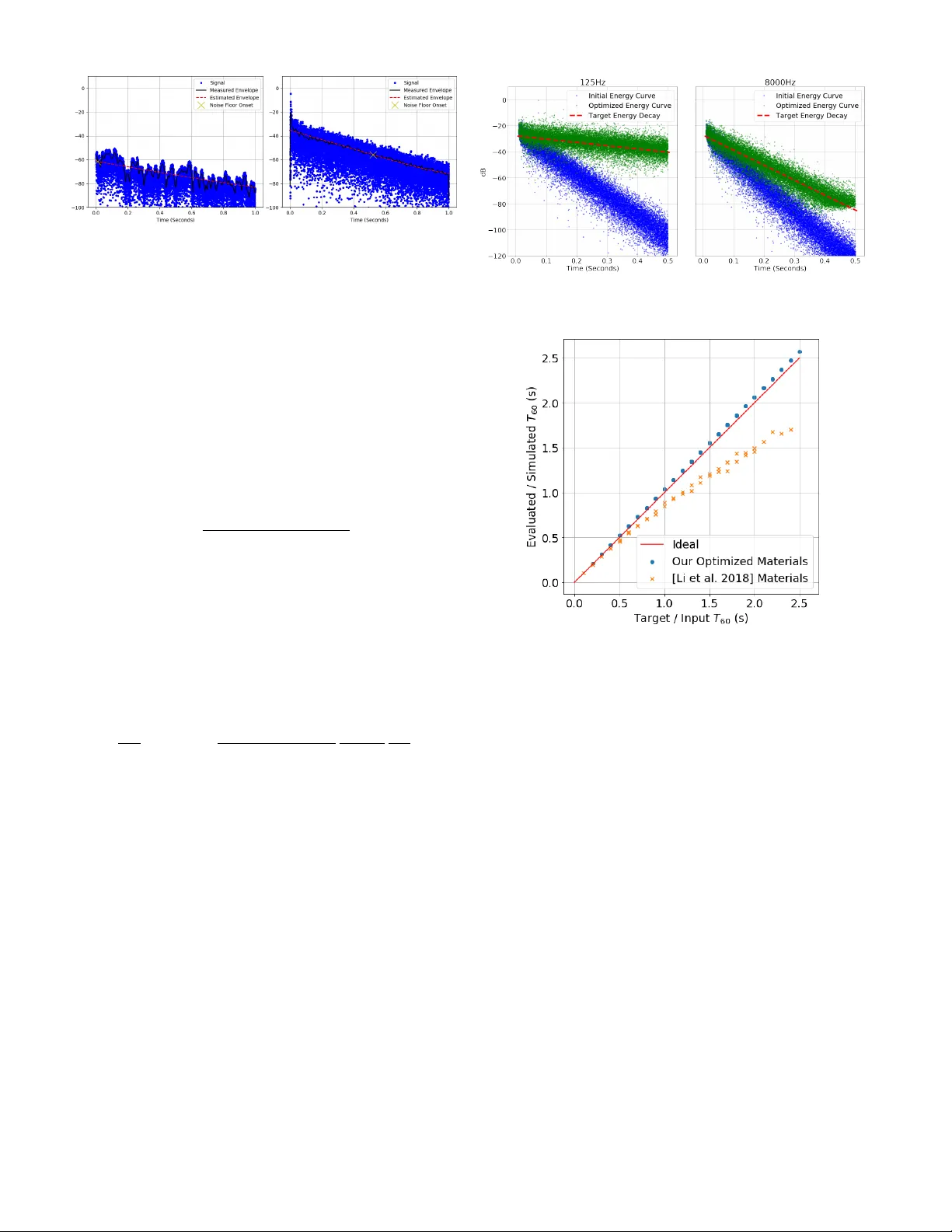
Scene-A w are A udio Render ing via Deep Acoustic Analysis Zhenyu T ang, Nicholas J . Br yan, Dingze yu Li, Timothy R. Langlois, and Dinesh Manocha Fig. 1: Giv en a natural sound in a real-world room that is recorded using a cellphone microphone (left), we estimate the acoustic material properties and the frequency equalization of the room using a novel deep learning approach (middle). W e use the estimated acoustic material properties for generating plausible sound effects in the virtual model of the room (right). Our approach is general and robust, and w orks well with commodity devices. Abstract — We present a new method to capture the acoustic characteristics of real-world rooms using commodity devices , and use the captured character istics to generate similar sounding sources with vir tual models. Given the captured audio and an approximate geometric model of a real-world room, we present a novel learning-based method to estimate its acoustic material proper ties. Our approach is based on deep neural networks that estimate the rev erber ation time and equalization of the room from recorded audio. These estimates are used to compute mater ial proper ties related to room reverber ation using a novel mater ial optimization objective. We use the estimated acoustic mater ial characteristics for audio rendering using interactiv e geometr ic sound propagation and highlight the performance on many real-world scenarios. We also perform a user study to ev aluate the perceptual similarity between the recorded sounds and our rendered audio. Index T erms —A udio render ing, audio lear ning, material optimization. 1 I N T R O D U C T I O N Auditory perception of recorded sound is strongly affected by the acoustic en vironment it is captured in. Concert halls are carefully designed to enhance the sound on stage, e ven accounting for the ef fects an audience of human bodies will ha ve on the propagation of sound [2]. Anechoic chambers are designed to remov e acoustic reflections and propagation ef fects as much as possible. Home theaters are designed with acoustic absorption and dif fusion panels, as well as with careful speaker and seating arrangements [47]. The same acoustic ef fects are important when creating immersiv e effects for virtual reality (VR) and augmented reality (AR) applications. It is well known that realistic sounds can improve a user’ s sense of presence and immersion [33]. There is considerable work on interac- tiv e sound propagation in virtual en vironments based on geometric and wa ve-based methods [7, 43, 53, 72]. Furthermore, these techniques are increasingly used to generate plausible sound ef fects in VR systems and games, including Microsoft Project Acoustics 1 , Oculus Spatializer 2 , and Steam Audio 3 . Howe ver , these methods are limited to synthetic scenes where an exact geometric representation of the scene and acous- tic material properties are known apriori. In this paper , we address the problem of rendering realistic sounds that are similar to recordings of real acoustic scenes. These capabil- • Zhenyu T ang and Dinesh Manocha ar e with the University of Maryland. E-mail: { zhy,dm } @cs.umd.edu. • Nicholas J. Bryan, Dingze yu Li and T imothy R. Langlois are with Adobe Resear ch. E-mail: { nibryan,dinli,tlangloi } @adobe.com. Manuscript r eceived xx xxx. 201x; accepted xx xxx. 201x. Date of Publication xx xxx. 201x; date of current version xx xxx. 201x. F or information on obtaining r eprints of this article, please send e-mail to: reprints@ieee .or g. Digital Object Identifier: xx.xxxx/TVCG.201x.xxxxxxx 1 https://aka.ms/acoustics 2 https://dev eloper .oculus.com/downloads/package/oculus-spatializer-unity 3 https://valv esoftware.github .io/steam-audio Project website https://gamma.umd.edu/pro/sound/sceneaware ities are needed for VR as well as AR applications [11], which often use recorded sounds. Foley artists often record source audio in en vi- ronments similar to the places the visual contents were recorded in. Similarly , creators of vocal content (e.g. podcasts, movie dialogue, or video voice-o vers), carefully re-record content made in different en vi- ronment or with dif ferent equipment to match the acoustic conditions. Howe ver, these processes are expensi v e, time-consuming, and cannot adapt to spatial listening location. There is strong interest in de v eloping automatic spatial audio synthesis methods. For VR or AR content creation, acoustic ef fects can also be captured with an impulse response (IR) – a compact acoustic description of how sound propagates from one location to another in a giv en scene. A given IR can be con volved with any virtual sound or dry sound to generate the desired acoustic effects. Howe ver , recording the IRs of real- world scenes can be challenging, especially for interactive applications. Many times special recording hardware is needed to record the IRs. Furthermore, the IR is a function of the source and listener positions and it needs to be re-recorded as either position changes. Our goal is to replace the step of recording an IR with an unobtrusi ve method that works on in-situ speech recordings and video signals and uses commodity de vices. This can be regarded as an acoustic analogy of visual relighting [13]: to light a new visual object in an image, traditional image based lighting methods require the capture of real- world illumination as an omnidirectional, high dynamic range (HDR) image. This light can be applied to the scene, as well as on a newly inserted object, making the object appear as if it w as alw ays in the scene. Recently , Gardner et al. [20] and Hold-Geoffroy et al. [25] proposed con v olutional neural network (CNN)-based methods to estimate HDR indoor or outdoor illumination from a single low dynamic range (LDR) image. These high-quality visual illumination estimation methods enable nov el interactiv e applications. Concurrent work from LeGendre et al. [34] demonstrates the ef fectiv eness on mobile de vices, enabling photorealistic mobile mixed reality e xperiences. In terms of audio “relighting” or reproduction, there hav e been se v- eral approaches proposed toward realistic audio in 360 ° images [29], Fig. 2: Our pipeline: Starting with an audio-video recording (left), we estimate the 3D geometric representation of the en vironment using standard computer vision methods. W e use the reconstructed 3D model to simulate ne w audio ef fects in that scene. T o ensure our simulation results perceptually match recorded audio in the scene, we automatically estimate two acoustic properties from the audio recordings: frequency-dependent rev erberation time or T 60 of the en vironment, and a frequency-dependent equalization curv e. The T 60 is used to optimize the frequency-dependent absorption coefficients of the materials in the scene. The frequency equalization filter is applied to the simulated audio, and accounts for the missing wa ve ef fects in geometrical acoustics simulation. W e use these parameters for interactiv e scene-aw are audio rendering (right). multi-modal estimation and optimization [52], and scene-aware audio in 360 ° videos [35]. Howev er , these approaches either require separate recording of an IR, or produce audio results that are perceptually dif- ferent from recorded scene audio. Important acoustic properties can be extracted from IRs, including the rev erberation time ( T 60 ), which is defined as the time it takes for a sound to decay 60 decibels [32], and the frequency-dependent amplitude le vel or equalization (EQ) [22]. Main Results: W e present nov el algorithms to estimate two important en vironmental acoustic properties from recorded sounds (e.g. speech). Our approach uses commodity microphones and does not need to cap- ture any IRs. The first property is the frequency-dependent T 60 . This is used to optimize absorption coef ficients for geometric acoustic (GA) simulators for audio rendering. Next, we estimate a frequency equaliza- tion filter to account for wa ve ef fects that cannot be modeled accurately using geometric acoustic simulation algorithms. This equalization step is crucial to ensuring that our GA simulator outputs perceptually match existing recorded audio in the scene. Estimating the equalization filter without an IR is challenging since it is not only speak er dependent, b ut also scene dependent, which poses extra dif ficulties in terms of dataset collection. For a model to predict the equalization filtering behavior accurately , we need a large amount of div erse speech data and IRs. Our key idea is a nov el dataset augmen- tation process that significantly increases room equalization v ariation. W ith robust room acoustic estimation as input, we present a nov el in verse material optimization algorithm to estimate the acoustic prop- erties. W e propose a new objecti v e function for material optimization and sho w that it models the IR decay beha vior better than the technique by Li et al. [35]. W e demonstrate our ability to add new sound sources in regular videos. Similar to visual relighting examples where new objects can be rendered with photorealistic lighting, we enable audio reproduction in any regular video with e xisting sound with applications for mixed reality experiences. W e highlight their performance on many challenging benchmarks. W e sho w the importance of matched T 60 and equalization in our perceptual user study § 5. In particular , our perceptual evaluation results show that: (1) Our T 60 estimation method is perceptually comparable to all past baseline approaches, ev en though we do not require an explicit measured IR; (2) Our EQ estimation method improv es the performance of our T 60 -only approach by a statistically significant amount ( ≈ 10 rating points on a 100 point scale); and (3) Our combined method ( T 60 +EQ) outperforms the average room IR ( T 60 = . 5 seconds with uniform EQ) by a statistically significant amount ( + 10 rating points) – the only reasonable comparable baseline we could concei v e that does not require an explicit IR estimate. T o the best of our knowledge, ours is the first method to predict IR equalization from raw speech data and validate its accurac y . Our main contributions include: • A CNN-based model to estimate frequency-dependent T 60 and equalization filter from real-world speech recordings. • An equalization augmentation scheme for training to improv e the prediction robustness. • A deriv ation for a new optimization objectiv e that better models the IR decay process for in verse materials optimization. • A user study to compare and v alidate our performance with cur - rent state-of-the-art audio rendering algorithms. Our study is used to ev aluate the perceptual similarity between the recorded sounds and our rendered audio. 2 R E L AT E D W O R K Cohesiv e audio in mixed reality en vironments (when there is a mix of real and virtual content), is more dif ficult than in fully virtual en- vironments. This stems from the difference between “Plausibility” in VR and “ Authenticity” in AR [29]. V isual cues dominate acoustic cues, so the perceptual dif ference between ho w audio sounds and the en vironment in which it is seen is smaller than the perceived en vi- ronment of two sounds. Recently , Li et al. introduced scene-aware audio to optimize simulator parameters to match the room acoustics from existing recordings [35]. By lev eraging visual information for acoustic material classification, Schissler et al. demonstrated realistic audio for 3D-reconstructed real-world scenes [52]. Howe ver , both of these methods still require e xplicit measurement of IRs. In contrast, our proposed pipeline works with an y input speech signal and commodity microphones. Sound simulation can be categorized into w av e-based methods and geometric acoustics. While wav e-based methods generally produce more accurate results, it remains an open challenge to build a real-time univ ersal wav e solver . Recent adv ances such as parallelization via rectangular decomposition [38], pre-computation acceleration struc- tures [36], and coupling with geometric acoustics [48, 73] are used for interactiv e applications. It is also possible to precompute lo w-frequenc y wa ve-based propagation ef fects in lar ge scenes [45], and to perceptually compress them to reduce runtime requirements [44]. Even with the mas- siv e speedups presented, and a real-time runtime engine, these methods still require tens of minutes to hours of pre-computation depending 10 2 10 3 10 4 Frequency (Hz) -60 -50 -40 -30 -20 -10 0 10 dB Simulated Response Recorded Response Fig. 3: The simulated and recorded frequency response in the same room at a sample rate of 44.1kHz is shown. Note that the recorded response has noticeable peaks and notches compared with the relati vely flat simulated response. This is mainly caused by room equalization. Missing proper room equalization leads to discrepancies in audio qual- ity and ov erall room acoustics. on the size of the scene and frequency range chosen, making them impractical for augmented reality scenarios and dif ficult to include in an optimization loop to estimate material parameters. With interacti v e applications as our goal, most game engines and VR systems tend to use geometric acoustic simulation methods [7, 53, 54, 72]. These algo- rithms are based on f ast ray tracing and perform specular and dif fuse reflections [50]. Some techniques have been proposed to approximate low-frequenc y dif fraction ef fects using ray-tracing [48, 66, 69]. Our ap- proach can be combined with any interactiv e audio simulation method, though our current implementation is based on bidirectional ray trac- ing [7]. The sound propagation algorithms can also be used for acoustic material design optimization for synthetic scenes [37]. The efficiency of deep neural netw orks has been shown in audio/video-related tasks that are challenging for traditional meth- ods [17, 21, 24, 61, 71]. Hershey et al. showed that it is feasible to use CNNs for large-scale audio classification problems [23]. Many deep neural networks require a large amount of training data. Sala- mon et al. used data augmentation to improv e en vironmental sound classification [49]. Similarly , Bryan estimates the T 60 and the direct-to- rev erberant ratio (DRR) from a single speech recording via augmented datasets [5]. T ang et al. trained CRNN models purely based on syn- thetic spatial IRs that generalize to real-world recordings [63 – 65]. W e strategically design an augmentation scheme to address the challenge of equalization’ s dependence on both IRs and speaker voice profiles, which is fully complimentary to all prior data-driv en methods. Acoustic simulators require a set of well-defined material proper- ties. The material absorption coefficient is one of the most important parameters [4], ranging from 0 (total reflection) to 1 (total absorption). When a reference IR is a vailable, it is straightforw ard to adjust room materials to match the energy decay of the simulated IR to the refer- ence IR [35]. Similarly , Ren et al. optimized linear modal analysis parameters to match the giv en recordings [46]. A probabilistic damping model for audio-material reconstruction has been presented for VR applications [60]. Unlike all pre vious methods which require a clean IR recording for accurate estimation and optimization of boundary materials, we infer typical material parameters including T 60 values and equalization from raw speech signals using a CNN-based model. Analytical gradients can significantly accelerate the optimization process. With similar optimization objectiv es, it was shown that addi- tional gradient information can boost the speed by a factor of ov er ten times [35, 52]. The speed gain shown by Li et al. [35] is impressive, and we further improv e the accuracy and speed of the formulation. More specifically , the original objectiv e function e v aluated energy decay rela- tiv e to the first ray recei ved (the direct sound if there were no obstacles). Howe ver, energy estimates can be noisy due to both the oscillatory T able 1: Notation and symbols used throughout the paper . T 60 Rev erberation time for sound ener gy to drop by 60dB. t Sound arriv al time. ρ Frequency dependent sound absorption coef ficient. e j Energy carried by a sound path j . β Air absorption coefficient. m Slope of the energy curv e en v elope. nature of audio as well as simulator noise. Instead, we optimize the slope of the best fit line of ray energies to the desired energy decay (defined by the T 60 ), which we found to be more robust. 3 D E E P A C O U S T I C A N A L Y S I S : O U R A L G O R I T H M In this section, we ov ervie w our proposed method for scene-aware audio rendering. W e begin by pro viding background information, discuss how we capture room geometry , and then proceed with discussing ho w we estimate the frequency dependent room rev erberation and equalization parameters directly from recorded speech. W e follow by discussing how we use the estimated acoustic parameters to perform acoustic materials optimization such that we calibrate our virtual acoustic model with real-world recordings. 3.1 Backgr ound T o explain the moti v ation of our approach, we briefly elaborate on the most dif ficult parts of previous approaches, upon which our method improv es. Previous methods require an impulse response of the en vi- ronment to estimate acoustic properties [35, 52]. Recording an impulse response is a non-trivial task. The most reliable methods in volve play- ing and recording Golay codes [19] or sine sweeps [18], which both play loud and intrusi ve audio signals. Also required are a fairly high- quality speaker and microphone with constant frequency response, small harmonic distortion and little crosstalk. The speaker and mi- crophone should be acoustically separated from surfaces, i.e., they shouldn’t be placed directly on tables (else surface vibrations could contaminate the signal). Clock drift between the source and micro- phone must be accounted for [6]. Alternativ ely , balloon pops or hand claps hav e been proposed for easier IR estimation, but require sig- nificant post-processing and still are very obtrusi ve [1, 56]. In short, correctly recording an IR is not easy , and makes it challenging to add audio in scenarios such as augmented reality , where the en vironment is not known beforehand and estimation must be done interactiv ely to preserve immersion. Geometric acoustics is a high-frequency approximation to the wa ve equation. It is a fast method, but assumes that wa v elengths are small compared to objects in the scene, while ignoring pressure ef fects [50]. It misses se veral important wav e ef fects such as dif fraction and room resonance. Diffraction occurs when sound paths bend around objects that are of similar size to the wavelength. Resonance is a pressure effect that happens when certain wa velengths are either reinforced or diminished by the room geometry: certain wavelengths create peaks or troughs in the frequency spectrum based on the positiv e or neg ativ e interference they create [12]. W e model these ef fects with a linear finite impulse response (FIR) equalization filter [51]. W e compute the discrete Fourier transform on the recorded IR over all frequencies, following [35]. Instead of filtering directly in the frequency domain, we design a linear phase EQ filter with 32ms delay to compactly represent this filter at 7 octave bin locations. W e then blindly estimate this compact representation of the frequency spectrum of the impulse response as discrete frequenc y gains, without specific kno wledge of the input sound or room geometry . This is a challenging estimation task. Since the con v olution of two signals (the IR and the input sound) is equi valent to multiplication in the frequency domain, estimating the frequency response of the IR is equivalent to estimating one multiplicative factor of a number without constraining the other . W e are relying on this approach to rec- Fig. 4: Network architecture for T 60 and EQ prediction. T wo models are trained for T 60 and EQ, which ha ve the same components except the output layers hav e dif ferent dimensions customized for the octav e bands they use. ognize a compact representation of the frequency response magnitude in different en vironments. 3.2 Geometry Reconstruction Giv en the background, we begin by first estimating the room geometry . In our experiments, we utilize the ARKit-based iOS app MagicPlan 4 to acquire the basic room geometry . A sample reconstruction is shown in Figure 5. W ith computer vision research e volving rapidly , we believ e constructing geometry proxies from video input will become e v en more robust and easily accessible [3, 74]. 3.3 Learning Re verberation and Equalization W e use a conv olutional neural netw ork (Figure 4) to predict room equal- ization and re verberation time ( T 60 ) directly from a speech recording. T raining requires a large number of speech recordings with kno wn T 60 and room equalization. The standard practice is to generate speech recordings from kno wn real-world or synthetic IRs [14, 28]. Unfortu- nately , large scale IR datasets do not currently exist due to the dif fi culty of IR measurement; most publicly available IR datasets ha v e fewer than 1000 IR recordings. Synthetic IRs are easy to obtain and can be used, but again lack w av e-based ef fects as well as other simulation deficien- cies. Recent work has addressed this issue by combining real-word IR measurements with augmentation to increase the di versity of e xisting real-world datasets [5]. This work, howev er , only addresses T 60 and DRR augmentation, and lacks a method to augment the frequency- equalization of existing IRs. T o address this, we propose a method to do this in Section 3.3.2. Beforehand, ho we ver , we discuss our neural network estimation method for estimating both T 60 and equalization. 3.3.1 Octav e-Based Prediction Most prior work takes the full-frequency range as input for predic- tion. F or example, one closely related work [5] only predicts one T 60 value for the entire frequency range (full-band). Howe ver , sound propagates and interacts with materials differently at different fre- quencies. T o this end, we define our learning targets over several 4 https://www .magicplan.app/ Fig. 5: W e use an off-the-shelf app called MagicPlan to generate geometry proxy . Input: a real-world room (left); Output: the captured 3D model of the room (right) without high-level details, which is used by the runtime geometric acoustic simulator . octav es. Specifically , we calculate T 60 at 7 sub-bands centered at { 125 , 250 , 500 , 1000 , 2000 , 4000 , 8000 } Hz. W e found prediction of T 60 at the 62.5Hz band to be unreliable due to lo w signal-to-noise ratio (SNR). During material optimization, we set the 62.5Hz T 60 value to the 125Hz value. Our frequency equalization estimation is done at 6 octav e bands centered at { 62 . 5 , 125 , 250 , 500 , 2000 , 4000 } Hz. As we describe in § 3.3.2, we compute equalization relativ e to the 1kHz band, so we do not estimate it. When applying our equalization filter, we set bands greater than or equal to 8kHz to − 50 dB. Giv en our target sampling rate of 16kHz and the limited content of speech in higher octav es, this did not af fect our estimation. 3.3.2 Data A ugmentation W e use the following datasets as the basis for our training and augmen- tation. • ACE Challenge: 70 IRs and noise audio [15]; • MIT IR Survey: 271 IRs [68]; • D APS dataset: 4.5 hours of 20 speakers’ speech (10 males and 10 females) [40]. First, we use the method in [5] to expand the T 60 and direct-to- rev erberant ratio (DRR) range of the 70 A CE IRs, resulting in 7000 synthetic IRs with a balanced T 60 distribution between 0.1–1.5 seconds. The ground truth T 60 estimates can be computed directly from IRs can be computed is a v ariety of w ays. W e follow the methodology of Karjalainen et al. [27] when computing the T 60 from real IRs with a measurable noise floor . This method was found to be the most rob ust estimator when computing the T 60 from real IRs in recent work [15]. The final composition of our dataset is listed in T able 2. While we know the common range of real-world T 60 values, there is limited literature gi ving statistics about room equalization. Therefore, we analyzed the equalization range and distribution of the 271 MIT surve y IRs as a guidance for data augmentation. The equalization of frequency bands is computed relative to the 1kHz octave. This is a common practice [70], unless expensi ve equipment is used to obtain calibrated acoustic pressure readings. For our equalization augmentation procedure, we first fit a normal distribution (mean and standard de viation) to each sub-band amplitude of the MIT IR dataset as sho wn in Figure 6. Gi ven this set of parametric model estimates, we iterate through our training and validation IRs. For each IR, we extract its original EQ. W e then randomly sample a target EQ according to our fit models (independently per frequency band), calculate the distance between the source and target EQ, and then design an FIR filter to compensate for the difference. For simplicity , we use the window method for FIR filter design [59]. Note, we do not require a perfect filter design method. W e simply need a procedure to increase the di versity of our data. Also note, we intentionally sample our augmented IRs to ha v e a lar ger v ariance than the recorded IRs to further increase the variety of our training data. W e compute the log Mel-frequenc y spectrogram for each four second audio clip, which is commonly used for speech-related tasks [9, 16]. W e (a) MIT IR survey equalization distrib ution by sub-band. (b) Original synthetic IR equalization. (c) T arget (MIT) IR equalization. (d) Augmented synthetic IR equalization. Fig. 6: Equalization augmentation. The 1000Hz sub-band is used as reference and has unit gain. W e fit normal distributions (red bell curves shown in (a)) to describe the EQ gains of MIT IRs. W e then apply EQs sampled from these distributions to our training set distribution in (b). W e observe that the augmented EQ distrib ution in (d) becomes more similar to the target distrib ution in (c). T able 2: Dataset composition. The training set and validation set are based on synthetic IRs and the test set is based on real IRs to guarantee model generalization. Clean speech files are also di vided in a way that speakers (“f1” for female speaker 1; “m10” for male speaker 10) in each dataset partition are different, to avoid the model learning the speaker’ s voice signature. Audio files are generated at a sample rate of 16kHz, which is sufficient to cov er the human voice’ s frequency range. Partition Noise Clean Speech IR T raining set (size: 56.5k) A CE ambient f5 ∼ f10, m5 ∼ m10 Synthetic IR (size: 4.5k) V alidation set (size: 19.5k) A CE ambient f3, f4, m3, m4 Synthetic IR (size: 1k) T est set (size: 18.5k) A CE ambient f1, f2, m1, m2 MIT survey IR (size: 271) use a Hann windo w of size 256 with 50% overlap during computation of the short-time Fourier transform (STFT) for our 16kHz samples. Then we use 32 Mel-scale bands and area normalization for Mel-frequency warping [62]. The spectrogram po wer is computed in decibels. This extraction process yields a 32 x 499 (frequency x time domain) matrix feature representation. All feature matrices are normalized by the mean and standard deviation of the training set. 3.3.3 Network Architecture and T raining W e propose using a network architecture dif fering only in the final layer for both T 60 and room equalization estimation. Six 2D con volutional layers are used sequentially to reduce both the time and frequency resolution of features until they ha ve approximately the same dimen- sion. Each conv layer is immediately followed by a rectified linear unit ( ReLU ) [41] activ ation function, 2D max pooling, and batch nor- malization. The output from conv layers is flattened to a 1D vector and connected to a fully connected layer of 64 units, at a dropout rate of 50% to lower the risk of ov erfitting. The final output layer has 7 fully connected units to predict a vector of length 7 for T 60 or 6 fully connected units to predict a vector of length 6 for frequenc y equaliza- tion. This network architecture is inspired by Bryan [5], where it w as used to predict full-band T 60 . W e updated the output layer to predict the more challenging sub-band T 60 , and also discov ered that the same architecture predicts equalization well. For training the network, we use the mean square error (MSE) with the AD AM optimizer [30] in Keras [10]. The maximum number of epochs is 500 with an early stopping mechanism. W e choose the model with the lowest v alidation error for further e valuation on the test set. Our model architecture is shown in Figure 4. 3.4 Acoustic Material Optimization Our goal is to optimize the material absorption coef ficients at the same octav e bands as our T 60 estimator in § 3.3.1 of a set of room materials to match the sub-band T 60 of the simulated sound with the target predicted in § 3.3. Ra y Energy . W e borrow notation from [35]. Briefly , a geometric acoustic simulator generates a set of sound paths, each of which carries an amount of sound energy . Each material m i in a scene is described by a frequency dependent absorption coefficient, ρ i . A path lea ving the source is reflected by a set of materials before it reaches the listener . The energy fraction that is recei v ed by the listener along path j is e j = β j N j ∏ k = 1 ρ m k , (1) where m k is the material the path intersects on the k t h bounce, N j is the number of surface reflections for path j , and β j accounts for air absorption (dependent on the total length of the path). Our goal is to optimize the set of absorption coef ficients ρ i to match the energy (a) 125Hz sub-band. (b) 8000Hz sub-band. Fig. 7: Ev aluating T 60 from signal en velope on lo w and high frequency bands of the same IR. Note that the SNR in the lo w frequency band is lower than the high frequency band. This makes T 60 ev aluation for lo w frequency bands less reliable, which partly e xplains the lar ger test error in low frequenc y sub-bands. distribution of the paths e j to that of the en vironment’ s IR. Again similar to [35], we assume the energy decrease of the IR follows an exponential curve, which is a linear decay in dB space. The slope of this decay line in dB space is m 0 = − 60 / T 60 . Objective Function. W e propose the follo wing objecti ve function: J ( ρ ) = ( m − m 0 ) 2 (2) where m is the best fit line of the ray energies on a decibel scale: m = n ∑ n i = 0 t i y i − ∑ n i = 0 t i ∑ n i = 0 y i n ∑ n i = 0 t 2 i −  ∑ n i = 0 t i  2 , (3) with y i = 10log 10 ( e i ) , which we found to be more robust than pre vious methods. Specifically , in comparison with Equation (3) in [35], we see that Li et al. tried to match the slope of the energies relati v e to e 0 , forcing e 0 to be at the origin on a dB scale. Howe v er , we only care about the ener gy decrea se, and not the absolute scale of the v alues from the simulator . W e found that allo wing the absolute scale to mov e and only optimizing the slope of the best fit line produces a better match to the target T 60 . W e minimize J using the L-BFGS-B algorithm [75]. The gradient of J is giv en by ∂ J ∂ ρ j = 2 ( m − m 0 ) nt i − ∑ n i = 0 t i n ∑ n i = 0 t 2 i −  ∑ n i = 0 t i  2 10 ln ( 10 ) e i ∂ e i ∂ ρ j (4) 4 A N A L Y S I S A N D A P P L I C AT I O N S 4.1 Analysis Speed. W e implement our system on an Intel Xeon(R) CPU @3.60GHz and an NVIDIA GTX 1080 T i GPU. Our neural network inference runs at 222 frames per second (FPS) on 4-second sliding windows of audio due to the compact design (only 18K trainable pa- rameters). Optimization runs twice as fast with our improved objecti v e function. The sound rendering is based on the real-time geometric bi-directional sound path tracing from Cao et al. [7]. Sub-band T 60 prediction. W e first ev aluate our T 60 blind estima- tion model and achie ve a mean absolute error (MAE) of 0.23s on the test set (MIT IRs). While the 271 IRs in the test set hav e a mean T 60 of 0.49s with a standard deviation (STD) of 0.85s at the 125Hz sub-band, the highest sub-band 8000Hz only has a mean T 60 of 0.33s with a STD of 0.24s, which reflects a narro w subset within our T 60 augmentation range. W e also notice that the validation MAE on ACE IRs is 0.12s, which indicates our v alidation set and the test set still come from dif- ferent distributions. Another error source is the inaccurate labeling of low-frequenc y sub-band T 60 as shown in Figure 7, b ut we do not filter any outliers in the test set. In addition, our data is intended to cov er frequency ranges up to 8000Hz, but human speech has less ener gy in high-frequency range [67], which results in low signal energy for these sub-bands, making it more difficult for learning. Fig. 8: Simulated energy curves before and after optimization (with target slope sho wn). Fig. 9: Stress test of our optimizer . W e uniformly sample T 60 between 0.2s and 2.5s and set it to be the tar get. The ideal I/O relationship is a straight line passing the origin with slope 1 . Our optimization results matches the ideal line much better than prior optimization method. Material Optimization. When we optimize the room material absorption coefficients according to the predicted T 60 of a room, our optimizer efficiently modifies the simulated energy curv e to a desired energy decay rate ( T 60 ) as shown in Figure 8. W e also try fixing the room configuration and set the target T 60 to v alues uniformly distributed between 0.2s and 2.5s, and e v aluate the T 60 of the simulated IRs. The relationship between the target and output T 60 is shown in Figure 9, in which our simulation closely matches the target, demonstrating that our optimization is able to match a wide range of T 60 values. T o test the real-world performance of our acoustic matching, we recorded ground truth IRs in 5 benchmark scenes, then use the method in [35], which requires a reference IR, and our method, which does not require an IR, for comparison. Benchmark scenes and results are summarized in T able 3. W e apply the EQ filter to the simulated IR as a last step. Overall, we obtain a prediction MAE of 3.42dB on our test set, whereas before augmentation, the MAE was 4.72dB under the same training condition, which confirms the ef fecti veness of our EQ augmentation. The perceptual impact of the EQ filter step is ev aluated in §5. 4.2 Comparisons W e compare our work with two related projects, Schissler et al. [52] and Kim et al. [29], where the high-level goal is similar to ours but the specific approach is different. Material optimization is a key step in our method and Schissler et al. [52]. One major dif ference is that we additionally compensate for wa ve effects explicitly with an equalization filter . Figure 10 shows T able 3: Benchmark results for acoustic matching. These real-world rooms are of different sizes and shapes, and contain a wide v ariety of acoustic materials such as brick, carpet, glass, metal, wood, plastic, etc., which make the problem acoustically challenging. W e compare our method with [35]. Our method does not require a reference IR and still obtains similar T 60 and EQ errors in most scenes compared with their method. W e also achiev e faster optimization speed. Note that the input audio to our method is already noisy and re v erberant, whereas [35] requires clean IR recording. All IR plots in the table have the same time and amplitude scale. Benchmark Scene Size ( m 3 ) 1100 (irregular) 1428 (12 × 17 × 7) 990 (11 × 15 × 6) 72 (4 × 6 × 3) 352 (11 × 8 × 4) # Main planes 6 6 6 11 6 Groundtruth IR (dB scale) Li et al. [35] IR (dB scale) Opt. time (s) 29 43 25 71 46 T 60 error (s) 0.11 0.23 0.08 0.02 0.10 EQ error (dB) 1.50 2.97 8.59 3.61 7.55 Ours IR (dB scale) Opt. time (s) 13 13 14 31 20 T 60 error (s) 0.14 0.12 0.10 0.04 0.24 EQ error (dB) 2.26 3.86 3.97 3.46 4.62 Fig. 10: W e show the effect of our equalization filtering on audio spectrograms, compared with Schissler et al. [52]. In the highlighted region, we are able to better reproduce the fast decay in the high- frequency range, closely matching the recorded sound. the difference in spectrograms, where the high frequenc y equalization was not properly accounted for . Our method better replicates the rapid decay in the high frequency range. For audio comparison, please refer to our supplemental video. W e also want to highlight the importance of optimizing T 60 . In [29], a CNN is used for object-based material classification. Default materials are assigned to a limited set of objects. Without optimizing specifically for the audio objectiv e, the resulting sound might not blend in seamlessly with the e xisting audio. In Figure 11, we sho w that our method produces audio that matches the decay tail better , whereas [29] produces a longer rev erb tail than the recorded ground truth. 4.3 Applications Acoustic Matching in Videos Gi ven a recorded video in an acous- tic en vironment, our method can analyze the room acoustic properties from noisy , rev erberant recorded audio in the video. The room geom- etry can be estimated from video [3], if the user has no access to the room for measurement. During post-processing, we can simulate sound that is similar to the recorded sound in the room. Moreover , virtual characters or speakers, such as the ones shown in Figure 1, can be added to the video, generating sound that is consistent with the real-world en vironment. Fig. 11: W e demonstrate the importance on T 60 optimization on the audio amplitude wav eform. Our method optimizes the material pa- rameters based on input audio and matches the tail shape and decay amplitude with the recorded sound, whereas the visual-based object materials from Kim et al. [29] failed to compensate for the audio effects. Real-time Immersive Augmented Reality A udio Our method works in a real-time manner and can be integrated into modern AR systems. AR devices are capable of capturing real-world geometry , and can stream audio input to our pipeline. At interactiv e rates, we can optimize and update the material properties, and update the room EQ filter as well. Our method is not hardware-dependent and can be used with any AR de vice (which provides geometry and audio) to enable a more immersiv e listening experience. Real-world Computer-Aided Acoustic Design Computer-aided design (CAD) software has been used for designing architecture acous- Fig. 12: A screenshot of MUSHRA-like web interface used in our user study . The design is from Cartwright et al. [8]. tics, usually before construction is done, in a predictiv e manner [31, 42]. But when gi ven an existing real-w orld en vironment, it becomes chal- lenging for traditional CAD software to adapt to current settings be- cause acoustic measurement can be tedious and error-prone. By using our method, room materials and EQ properties can be estimated from simple input, and can be further fed to other acoustic design applications in order to impro ve the room acoustics such as material replacement, source and listener placement [39], and soundproofing setup. 5 P E R C E P T UA L E VA L UAT I O N W e perceptually e v aluated our approach using a critical listening test. For this test, we studied the perceptual similarity of a reference speech recording with speech recordings con v olved with simulated impulse responses. W e used the same speech content for the reference and all stimuli under testing and e v aluated how well we can reconstruct the same identical speech content in a giv en acoustic scene. This is useful for understanding the absolute performance of our approach compared to the ground truth results. 5.1 Design and Procedure For our test, we adopted the multiple stimulus with hidden reference and anchor (MUSHRA) methodology from the ITU-R BS.1534-3 rec- ommendation [57]. MUSHRA pro vides a protocol for the subjectiv e assessment of intermediate quality lev el of audio systems [57] and has been adopted for a wide v ariety of audio processing tasks such as audio coding, source separation, and speech synthesis ev aluation [8, 55]. In a single MUSHRA trial, participants are presented with a high- quality reference signal and asked to compare the quality (or similarity) of three to twelve stimuli on a 0-100 point scale using a set of vertical sliders as shown in Figure 12. The stimuli must contain a hidden reference (identical to the explicit reference), tw o anchor conditions – low-quality and high-quality , and any additional conditions under study (maximum of nine). The hidden reference and anchors are used to help the participants calibrate their ratings relative to one another , as well as to filter out inaccurate assessors in a post-screening process. MUSHRA tests serve a similar purpose to mean opinion (MOS) score tests [58], but requires fe wer participants to obtain results that are statistically significant. W e performed our studies using Amazon Mechanical T urk (AMT), resulting in a MUSHRA-like protocol [8]. In recent years, web-based MUSHRA-like tests have become a standard methodology and hav e been shown to perform equi valently to full, in-person tests [8, 55]. 5.2 P articipants W e recruited 269 participants on AMT to rate one or more of our fiv e acoustic scenes under testing follo wing the approach proposed by Cartwright et al. [8]. T o increase the quality of the e valuation, we pre-screened the participants for our tests. T o do this, we first required that all participants have a minimum number of 1000 approv ed Human Intelligence T ask (HITs) assignments and hav e had at least 97 percent of all assignments approv ed. Second, all participants must pass a hearing screening test to verify the y are listening ov er devices with an adequate frequency response. This was performed by asking participants to listen to two separate eight second recordings consisting of a 55Hz tone, a 10kHz tone and zero to six tones of random frequency . If any user failed to count the number of tones correctly after two or more attempts, they were not allowed to proceed. Out of the 269 participants who attempted our test, 261 participants passed. 5.3 T raining After ha ving passed our hearing screening test, each user was presented with a one page training test. For this, the participant was provided two sets of recordings. The first set of training recordings consisted of three recordings: a reference, a low-quality anchor , and a high-quality anchor . The second set of training recordings consisted of the full set of recordings used for the gi ven MUSHRA trail, albeit without the vertical sliders present. T o proceed to the actual test, participants were required to listen to each recording in full. In total, we estimated the training time to be approximately two minutes. 5.4 Stimuli For our test conditions, we simulated five different acoustic scenes. For each scene, a separate MUSHRA trial was created. In AMT lan- guage, each scene was presented as a separate HIT per user . For each MUSHRA trial or HIT , we tested the follo wing stimuli: hidden refer- ence, low-quality anchor, mid-quality anchor , baseline T 60 , Baseline T 60 +EQ, proposed T 60 , and proposed T 60 +EQ. As noted by the ITU-R BS.1534-3 specification [57], both the ref- erence and anchors hav e a significant effect on the test results, must resemble the artifacts from the systems, and must be designed care- fully . For our work, we set the hidden reference as an identical copy of the explicit reference (required), which consisted of speech con- volv ed with the ground truth IR for each acoustic scene. Then, we set the low-quality anchor to be completely anechoic, non-reverberated speech. W e set the mid-quality anchor to be speech conv olv ed with an impulse response with a 0.5 second T 60 (typical conference room) across frequencies, and uniform equalization. For our baseline comparison, we included tw o baseline approaches following previous work [35]. More specifically , our Baseline T 60 lev erages the geometric acoustics method proposed by Cao et al. [7] as well as the materials analysis calibration method of Li et al. [35]. Our Baseline T 60 +EQ extends this and includes the additional frequency equalization analysis [35]. These two baselines directly correspond to the proposed materials optimization (Proposed T 60 ) and equalization prediction subsystems (Proposed T 60 +EQ) in our work. The key differ - ence is that we estimate the parameters necessary for both steps blindly fr om speec h . 5.5 User Stud y Results When we analyzed the results of our listening test, we post-filtered the results following the ITU-R BS.1534-3 specification [57]. More specifically , we excluded assessors if they • rated the hidden reference condition for > 15% of the test items lower than a score of 90 • or , rated the mid-range (or lo w-range) anchor for more than 15% of the test items higher than a score of 90. Using this post-filtering, we reduce our collected data down to 70 unique participants and 108 unique test trials, spread across our five acoustic scene conditions. Among these participants, 24 are females and 46 are males, with an average age of 36.0 and a standard deviation of 10.2 years. W e show the box plots of our results in Figure 13. The median ratings for each stimulus include: Baseline T 60 (62.0), Baseline T 60 +EQ (85.0), Low-Anchor (40.5), Mid-Anchor (59.0), Proposed T 60 (61.5), Proposed T 60 +EQ (71.0), and Hidden Reference (99.5). As seen, the Low-Anchor and Hidden Reference outline the range of user scores for our test. In Fig. 13: Box plot results for our listening test. Participants were asked to rate how similar each recording was to the explicit reference. All recordings hav e the same content, but different acoustic conditions. Note our proposed T 60 and T 60 +EQ are both better than the Mid-Anchor by a statistically significant amount ( ≈ 10 rating points on a 100 point scale). terms of baseline approaches, the Proposed T 60 +EQ method achie ves the highest ov erall listening test performance. W e then see that our proposed T 60 method and T 60 +EQ method outperform the mid-anchor . Our proposed T 60 method is comparable to the baseline T 60 method, and our proposed T 60 +EQ method outperforms our proposed T 60 -only method. T o understand the statistical significance, we performed a repeated measures analysis of v ariance (ANO V A) to compare the effect of our stimuli on user ratings. The Hidden Reference and Low-Anchor are for calibration and filtering purposes and are not included in the following statistical tests, leaving 5 groups for comparison. Bartlett’ s test did not show a violation of homogeneity of variances ( χ 2 = 4 . 68 , p = 0 . 32 ). A one-way repeated measures ANO V A sho ws significant differences ( F ( 4 , 372 ) = 29 . 24 , p < 0 . 01 ) among group mean ratings. T o iden- tify the source of differences, we further conduct multiple post-hoc paired t-tests with Bonferroni correction [26]. W e are able to ob- serve follo wing results: a) There is no significant dif ference between Baseline T 60 and Proposed T 60 ( t ( 186 ) = − 1 . 72 , p = 0 . 35 ), suggesting that we cannot reject the null hypothesis of identical av erage scores between prior work (which uses manually measured IRs) and our work; b) There is a significant difference between Baseline T 60 +EQ and Proposed T 60 +EQ ( t ( 186 ) = − 5 . 09 , p < 0 . 01 ), suggesting our EQ method has a statistically different average (lower); c) There is a significant difference between Proposed T 60 and Proposed T 60 +EQ ( t ( 186 ) = − 2 . 91 , p = 0 . 02 ), suggesting our EQ method significantly improv es performance compared to our proposed T 60 -only subsystem; d) There is a significant difference between Mid-Anchor and Proposed T 60 +EQ ( t ( 186 ) = − 3 . 78 , p < 0 . 01 ), suggesting our method is statis- tically dif ferent (higher performing) on a verage than simply using an av erage room T 60 and uniform equalization. In summary , we see that our proposed T 60 computation method is comparable to prior work, albeit we perform such estimation directly from a short speech recording rather than relying on intrusiv e IR mea- surement schemes. Further, our proposed complete system (Proposed T 60 +EQ) outperforms both the mid-anchor and proposed T 60 system alone, demonstrating the value of EQ estimation. Finally , we note our proposed T 60 +EQ method does not perform as well as prior work, largely due to the EQ estimation subsystem. This result, howe ver , is expected as prior work requires manual IR measurements, which result in perfect EQ estimation. This is in contrast to our work, which directly estimates both T 60 and EQ parameters from recorded speech, enabling a drastically improv ed interaction paradigm for matching acoustics in sev eral applications. 6 C O N C L U S I O N A N D F U T U R E W O R K W e present a new pipeline to estimate, optimize, and render immersive audio in video and mix ed reality applications. W e present nov el algo- rithms to estimate two important acoustic environment characteristics – the frequency-dependent re verberation time and equalization filter of a room. Our multi-band octa ve-based prediction model works in tandem with our equalization augmentation and provides robust input to our improv ed materials optimization algorithm. Our user study validates the perceptual importance of our method. T o the best of our kno wledge, our method is the first method to predict IR equalization from raw speech data and validate its accurac y . Limitations and Future Work. T o achiev e a perfect acoustic match, one would expect the real-world validation error to be zero. In reality , zero error is only a suf ficient but not necessary condition. In our ev aluation tests, we observe that small validation errors still allo w for plausible acoustic matching. While reducing the prediction error is an important direction, it is also useful to in vestigate the perceptual error threshold for acoustic matching for different tasks or applications. Moreov er , temporal prediction coherence is not in our e v aluation pro- cess. This implies that gi ven a sliding windows of audio recordings, our model might predict temporally incoherent T 60 values. One interesting problem is to utilize this coherence to improve the prediction accurac y as a future direction. Modeling real-world characteristics in simulation is a non-trivial task – as in previous w ork along this line, our simulator does not fully recreate the real world in terms of precise details. For example, we did not consider the speaker or microphone response curve in our simulation. In addition, sound sources are modeled as omnidirectional sources [7], where real sources exhibit certain directional patterns. It remains an open research challenge to perfectly replicate and simulate our real world in a simulator . Like all data-driv en methods, our learned model performs best on the same kind of data on which it was trained. Augmentation is useful because it generalizes the e xisting dataset so that the learned model can extrapolate to unseen data. Howe ver , defining the range of augmenta- tion is not straightforward. W e set the MIT IR dataset as the baseline for our augmentation process. In certain cases, this assumption might not generalize well to estimate the extreme room acoustics. W e need to design better and more uni versal augmentation training algorithms. Our method focused on estimation from speech signals, due to their pervasi veness and importance. It would be useful to explore ho w well the estimation could work on other audio domains, especially when in- terested in frequency ranges outside typical human speech. This could further increase the usefulness of our method, e.g., if we could estimate acoustic properties from ambient/HV A C noise instead of requiring a speech signal. A C K N OW L E D G M E N T S The authors would like to thank Chunxiao Cao for sharing the bidi- rectional sound simulation code, James T raer for sharing the MIT IR dataset, and anonymous revie wers for their constructiv e feedback. This work was supported in part by AR O grant W911NF-18-1-0313, NSF grant #1910940, Adobe Research, Facebook, and Intel. R E F E R E N C E S [1] J. S. Abel, N. J. Bryan, P . P . Huang, M. Kolar , and B. V . Pentcheva. Estimating room impulse responses from recorded balloon pops. In Audio Engineering Society Con vention 129 . Audio Engineering Society , 2010. [2] M. Barron. Auditorium acoustics and ar chitectur al design . E & FN Spon, 2010. [3] M. Bloesch, J. Czarno wski, R. Clark, S. Leutenegger , and A. J. Davison. Codeslam - learning a compact, optimisable representation for dense visual slam. In The IEEE Conference on Computer V ision and P attern Recognition (CVPR) , June 2018. [4] I. Bork. A comparison of room simulation software-the 2nd round robin on room acoustical computer simulation. Acta Acustica united with Acustica , 86(6):943–956, 2000. [5] N. J. Bryan. Impulse response data augmentation and deep neural net- works for blind room acoustic parameter estimation. arXiv preprint arXiv:1909.03642 , 2019. [6] N. J. Bryan, J. S. Abel, and M. A. Kolar . Impulse response measurements in the presence of clock drift. In Audio Engineering Society Convention 129 . Audio Engineering Society , 2010. [7] C. Cao, Z. Ren, C. Schissler, D. Manocha, and K. Zhou. Bidirectional sound transport. The Journal of the Acoustical Society of America , 141(5):3454–3454, 2017. [8] M. Cartwright, B. Pardo, G. J. Mysore, and M. Hoffman. Fast and easy crowdsourced perceptual audio ev aluation. In 2016 IEEE International Confer ence on Acoustics, Speech and Signal Pr ocessing (ICASSP) , pp. 619–623. IEEE, 2016. [9] L. Chen, Z. Li, R. K Maddox, Z. Duan, and C. Xu. Lip movements generation at a glance. In The Eur opean Confer ence on Computer V ision (ECCV) , September 2018. [10] F . Chollet et al. Keras. https://keras.io , 2015. [11] A. I. Conference. Audio for virtual and augmented reality . AES Proceed- ings , 2018. [12] T . J. Cox, P . D’Antonio, and M. R. A vis. Room sizing and optimization at low frequencies. Journal of the Audio Engineering Society , 52(6):640–651, 2004. [13] P . Debe v ec. Image-based lighting. IEEE Computer Graphics and Applica- tions , 22(2):26–34, 2002. [14] M. Doulaty , R. Rose, and O. Siohan. Automatic optimization of data perturbation distributions for multi-style training in speech recognition. In Spoken Language T echnology W orkshop , 2017. [15] J. Eaton, N. D. Gaubitch, A. H. Moore, P . A. Naylor, J. Eaton, N. D. Gaubitch, A. H. Moore, P . A. Naylor , N. D. Gaubitch, J. Eaton, et al. Esti- mation of room acoustic parameters: The ace challenge. IEEE/ACM T rans- actions on A udio, Speech and Language Processing (T ASLP) , 24(10):1681– 1693, 2016. [16] S. E. Eskimez, P . Soufleris, Z. Duan, and W . Heinzelman. Front-end speech enhancement for commercial speaker verification systems. Speech Communication , 99:101–113, 2018. [17] C. Evers, A. H. Moore, and P . A. Naylor . Acoustic simultaneous lo- calization and mapping (a-slam) of a moving microphone array and its surrounding speakers. In 2016 IEEE International Conference on Acous- tics, Speech and Signal Pr ocessing (ICASSP) , pp. 6–10. IEEE, 2016. [18] A. Farina. Simultaneous measurement of impulse response and distortion with a swept-sine technique. In Audio Engineering Society Convention 108 . Audio Engineering Society , 2000. [19] S. Foster . Impulse response measurement using golay codes. In ICASSP’86. IEEE International Conference on Acoustics, Speech, and Signal Pr ocessing , v ol. 11, pp. 929–932. IEEE, 1986. [20] M.-A. Gardner , K. Sunkavalli, E. Y umer , X. Shen, E. Gambaretto, C. Gagn ´ e, and J.-F . Lalonde. Learning to predict indoor illumination from a single image. arXiv preprint , 2017. [21] S. Gharib, H. Derrar, D. Niizumi, T . Senttula, J. T ommola, T . Heittola, T . V irtanen, and H. Huttunen. Acoustic scene classification: A competition revie w . In IEEE 28th International W orkshop on Machine Learning for Signal Pr ocessing (MLSP) , pp. 1–6. IEEE, 2018. [22] C. Hak, R. W enmaekers, and L. V an Luxembur g. Measuring room impulse responses: Impact of the decay range on deriv ed room acoustic parameters. Acta Acustica united with Acustica , 98(6):907–915, 2012. [23] S. Hershey , S. Chaudhuri, D. P . Ellis, J. F . Gemmeke, A. Jansen, R. C. Moore, M. Plakal, D. Platt, R. A. Saurous, B. Seybold, et al. Cnn ar- chitectures for large-scale audio classification. In IEEE International Confer ence on Acoustics, Speech and Signal Pr ocessing (ICASSP) , pp. 131–135. IEEE, 2017. [24] G. Hinton, L. Deng, D. Y u, G. Dahl, A.-r . Mohamed, N. Jaitly , A. Senior, V . V anhoucke, P . Nguyen, B. Kingsbury , et al. Deep neural networks for acoustic modeling in speech recognition. IEEE Signal pr ocessing magazine , 29, 2012. [25] Y . Hold-Geoffroy , K. Sunkav alli, S. Hadap, E. Gambaretto, and J.-F . Lalonde. Deep outdoor illumination estimation. In Pr oceedings of the IEEE Confer ence on Computer V ision and P attern Recognition , pp. 7312– 7321, 2017. [26] S. Holm. A simple sequentially rejectiv e multiple test procedure. Scandi- navian journal of statistics , pp. 65–70, 1979. [27] M. Karjalainen, P . Antsalo, A. Makivirta, T . Peltonen, and V . V alimaki. Estimation of modal decay parameters from noisy response measurements. In Audio Engineering Society Con vention 110 . Audio Engineering Society , 2001. [28] C. Kim, A. Misra, K. Chin, T . Hughes, A. Narayanan, T . N. Sainath, and M. Bacchiani. Generation of large-scale simulated utterances in virtual rooms to train deep-neural networks for far -field speech recognition in google home. In Interspeech , 2017. [29] H. Kim, L. Remaggi, P . Jackson, and A. Hilton. Immersiv e spatial audio reproduction for vr/ar using room acoustic modelling from 360 images. Pr oceedings IEEE VR2019 , 2019. [30] D. P . Kingma and J. Ba. Adam: A method for stochastic optimization. arXiv pr eprint arXiv:1412.6980 , 2014. [31] M. Kleiner , P . Sv ensson, and B.-I. Dalenb ¨ ack. Auralization: experiments in acoustical cad. In A udio Engineering Society Convention 89 . Audio Engineering Society , 1990. [32] H. Kuttruf f. Room Acoustics . T aylor & Francis Group, London, U. K., 6th ed., 2016. [33] P . Larsson, D. V astfjall, and M. Kleiner. Better presence and performance in virtual en vironments by improved binaural sound rendering. In V irtual, Synthetic, and Entertainment Audio confer ence , Jun 2002. [34] C. LeGendre, W .-C. Ma, G. Fyffe, J. Flynn, L. Charbonnel, J. Busch, and P . Debe v ec. Deeplight: Learning illumination for unconstrained mobile mixed reality . In Pr oceedings of the IEEE Confer ence on Computer V ision and P attern Recognition , pp. 5918–5928, 2019. [35] D. Li, T . R. Langlois, and C. Zheng. Scene-aware audio for 360 ° videos. ACM T rans. Graph. , 37(4), 2018. [36] R. Mehra, A. Rungta, A. Golas, M. Lin, and D. Manocha. W ave: Interac- tiv e wa ve-based sound propagation for virtual en vironments. IEEE trans- actions on visualization and computer graphics , 21(4):434–442, 2015. [37] N. Morales and D. Manocha. Ef ficient wave-based acoustic material design optimization. Computer-Aided Design , 78:83–92, 2016. [38] N. Morales, R. Mehra, and D. Manocha. A parallel time-domain wave simulator based on rectangular decomposition for distributed memory architectures. Applied Acoustics , 97:104–114, 2015. [39] N. Morales, Z. T ang, and D. Manocha. Receiver placement for speech enhancement using sound propagation optimization. Applied Acoustics , 155:53–62, 2019. [40] G. J. Mysore. Can we automatically transform speech recorded on com- mon consumer de vices in real-world en vironments into professional pro- duction quality speech?a dataset, insights, and challenges. IEEE Signal Pr ocessing Letters , 22(8):1006–1010, 2014. [41] V . Nair and G. E. Hinton. Rectified linear units improv e restricted boltz- mann machines. In Proceedings of the 27th international conference on machine learning (ICML-10) , pp. 807–814, 2010. [42] S. Pelzer , L. Asp ¨ ock, D. Schr ¨ oder , and M. V orl ¨ ander . Integrating real-time room acoustics simulation into a cad modeling software to enhance the architectural design process. Buildings , 4(2):113–138, 2014. [43] N. Raghuvanshi and J. Snyder . Parametric wav e field coding for pre- computed sound propagation. ACM T ransactions on Graphics (TOG) , 33(4):38, 2014. [44] N. Raghuvanshi and J. Sn yder. Parametric wave field coding for precom- puted sound propagation. A CM T rans. Graph. , 33(4):38:1–38:11, July 2014. [45] N. Raghuvanshi, J. Snyder , R. Mehra, M. Lin, and N. Govindaraju. Pre- computed wave simulation for real-time sound propagation of dynamic sources in complex scenes. ACM T rans. Gr aph. , 29(4):68:1–68:11, July 2010. [46] Z. Ren, H. Y eh, and M. C. Lin. Example-guided physically based modal sound synthesis. ACM T r ansactions on Graphics (T OG) , 32(1):1, 2013. [47] L. Rizzi, G. Ghelfi, and M. Santini. Small-rooms dedicated to music: From room response analysis to acoustic design. In Audio Engineering Society Con vention 140 . Audio Engineering Society , 2016. [48] A. Rungta, C. Schissler , N. Rewk owski, R. Mehra, and D. Manocha. Diffraction kernels for interactive sound propagation in dynamic envi- ronments. IEEE T ransactions on V isualization and Computer Gr aphics , 24(4):1613–1622, 2018. [49] J. Salamon and J. P . Bello. Deep conv olutional neural networks and data augmentation for environmental sound classification. IEEE Signal Pr ocessing Letters , 24(3):279–283, 2017. [50] L. Savioja and U. P . Svensson. Overview of geometrical room acoustic modeling techniques. The Journal of the Acoustical Society of America , 138(2):708–730, 2015. doi: 10 . 1121/1. 4926438 [51] R. W . Schafer and A. V . Oppenheim. Discrete-time signal pr ocessing . Prentice Hall Englew ood Cliffs, NJ, 1989. [52] C. Schissler, C. Loftin, and D. Manocha. Acoustic classification and optimization for multi-modal rendering of real-world scenes. IEEE Tr ans- actions on V isualization and Computer Graphics , 24(3):1246–1259, 2017. [53] C. Schissler and D. Manocha. Interactiv e sound propagation and rendering for lar ge multi-source scenes. A CM Tr ansactions on Graphics (T OG) , 36(1):2, 2017. [54] C. Schissler and D. Manocha. Interacti ve sound rendering on mobile devices using ray-parameterized rev erberation filters. arXiv pr eprint arXiv:1803.00430 , 2018. [55] M. Schoeffler , F .-R. St ¨ oter , B. Edler , and J. Herre. T owards the next generation of web-based experiments: A case study assessing basic audio quality following the itu-r recommendation bs. 1534 (mushra). In 1st W eb Audio Confer ence , pp. 1–6, 2015. [56] P . Seetharaman and S. P . T arzia. The hand clap as an impulse source for measuring room acoustics. In Audio Engineering Society Con vention 132 . Audio Engineering Society , 2012. [57] B. Series. Recommendation ITU-R BS. 1534-3 method for the subjective assessment of intermediate quality lev el of audio systems. International T elecommunication Union Radio Communication Assembly , 2014. [58] P . Series. Methods for objective and subjecti ve assessment of speech and video quality . International T elecommunication Union Radiocommunica- tion Assembly , 2016. [59] J. O. Smith III. Spectral Audio Signal Pr ocessing . 01 2008. [60] A. Sterling, N. Rewko wski, R. L. Klatzky , and M. C. Lin. Audio-material reconstruction for virtualized reality using a probabilistic damping model. IEEE transactions on visualization and computer graphics , 25(5):1855– 1864, 2019. [61] A. Sterling, J. Wilson, S. Lowe, and M. C. Lin. Isnn: Impact sound neural network for audio-visual object classification. In Pr oceedings of the Eur opean Confer ence on Computer V ision (ECCV) , pp. 555–572, 2018. [62] S. S. Stev ens, J. V olkmann, and E. B. Newman. A scale for the measure- ment of the psychological magnitude pitch. The Journal of the Acoustical Society of America , 8(3):185–190, 1937. [63] Z. T ang, L. Chen, B. W u, D. Y u, and D. Manocha. Improving rev er- berant speech training using dif fuse acoustic simulation. arXiv preprint arXiv:1907.03988 , 2019. [64] Z. T ang, J. Kanu, K. Hogan, and D. Manocha. Regression and classification for direction-of-arriv al estimation with con volutional recurrent neural networks. In Interspeech , 2019. [65] Z. T ang, H.-Y . Meng, and D. Manocha. Low-frequency compensated synthetic impulse responses for improved far -field speech recognition. arXiv pr eprint arXiv:1910.10815 , 2019. [66] M. T aylor , A. Chandak, Q. Mo, C. Lauterbach, C. Schissler, and D. Manocha. Guided multivie w ray tracing for fast auralization. IEEE T r ansactions on V isualization and Computer Graphics , 18:1797–1810, 2012. [67] I. R. T itze, L. M. Maxfield, and M. C. W alker. A formant range profile for singers. Journal of V oice , 31(3):382.e9 – 382.e13, 2017. [68] J. Traer and J. H. McDermott. Statistics of natural rev erberation enable perceptual separation of sound and space. Pr oceedings of the National Academy of Sciences , 113(48):E7856–E7865, 2016. [69] N. Tsingos, T . Funkhouser, A. Ngan, and I. Carlbom. Modeling acous- tics in virtual environments using the uniform theory of dif fraction. In Pr oceedings of the 28th Annual Conference on Computer Gr aphics and Interactive T ec hniques , pp. 545–552. A CM, 2001. [70] V . V ¨ alim ¨ aki and J. Reiss. All about audio equalization: Solutions and frontiers. Applied Sciences , 6(5):129, 2016. [71] T . V irtanen, M. D. Plumbley , and D. Ellis. Computational analysis of sound scenes and events . Springer, 2018. [72] M. V orl ¨ ander . Simulation of the transient and steady-state sound propaga- tion in rooms using a new combined ray-tracing/image-source algorithm. The Journal of the Acoustical Society of America , 86(1):172–178, 1989. [73] H. Y eh, R. Mehra, Z. Ren, L. Antani, D. Manocha, and M. Lin. W ave-ray coupling for interactiv e sound propagation in large complex scenes. ACM T r ansactions on Graphics (T OG) , 32(6):165, 2013. [74] S. Zhi, M. Bloesch, S. Leutenegger , and A. J. Davison. Scenecode: Monocular dense semantic reconstruction using learned encoded scene representations. In The IEEE Conference on Computer V ision and P attern Recognition (CVPR) , June 2019. [75] C. Zhu, R. H. Byrd, P . Lu, and J. Nocedal. Algorithm 778: L-bfgs-b: Fortran subroutines for large-scale bound-constrained optimization. ACM T r ans. Math. Softw . , 23(4):550–560, Dec. 1997.