Improved error rates for sparse (group) learning with Lipschitz loss functions

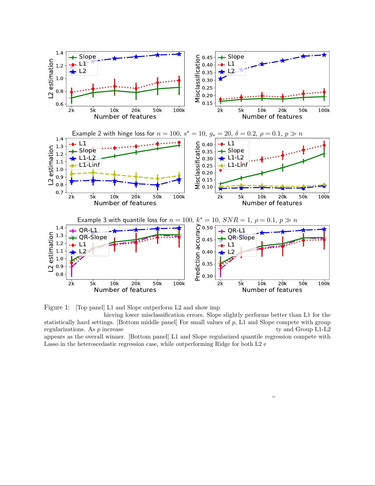
Impro v ed error rates for sparse (group) learning with Lipsc hitz loss functions An toine Dedieu Septem b er 23, 2021 Abstract W e study a family of sparse estimators deﬁned as minimizers of some empirical Lipsc hitz loss function—whic h include the hinge los s, the logistic loss and the quan tile regression loss—with a con vex, sparse or group-sparse regularization. In particular, we consider the L1 norm on the co eﬃcien ts, its sorted Slop e version, and the Group L1-L2 extension. W e prop ose a new theoretical framework that uses common assumptions in the literature to simultaneously derive new high-dimensional L2 estimation upper b ounds for all three regularization schemes. F or L1 and Slope regularizations, our b ounds scale as ( k ∗ /n ) log ( p/k ∗ )— n × p is the size of the design matrix and k ∗ the dimension of the theoretical loss minimizer β ∗ —and matc h the optimal minimax rate achiev ed for the least-squares case. F or Group L1-L2 regularization, our bounds scale as ( s ∗ /n ) log ( G/s ∗ ) + m ∗ /n — G is the total n umber of groups and m ∗ the num b er of co eﬃcien ts in the s ∗ groups whic h contain β ∗ —and impro ve ov er the least-squares case. W e sho w that, when the signal is strongly group-sparse, Group L1-L2 is sup erior to L1 and Slop e. In addition, we adapt our approach to the sub-Gaussian linear regression framework and reac h the optimal minimax rate for Lasso, and an improv ed rate for Group-Lasso. Finally , we release an accelerated proximal algorithm that computes the nine main con vex estimators of in terest when the num b er of v ariables is of the order of 100 , 000 s . 1 In tro duction W e consider a training data of indep enden t samples { ( x i , y i ) } n i =1 , ( x i , y i ) ∈ R p × Y from a distribution P ( X , y ). W e ﬁx a loss f and consider a theoretical minimizer β ∗ of the theoretical loss L ( β ) = E ( f ( h x , β i ; y )): β ∗ ∈ argmin β ∈ R p E ( f ( h x , β i ; y )) . (1) In the rest of this pap er, f ( ., y ) will b e assumed to b e Lipschitz and to admit a subgradient. W e denote k ∗ = k β ∗ k 0 the num b er of non-zeros coeﬃcients of the theoretical minimizer and R = k β ∗ k 1 its L1 norm. W e consider the L1-constrained learning problem min β ∈ R p : k β k 1 ≤ 2 R 1 n n X i =1 f ( h x i , β i ; y i ) + Ω( β ) , (2) where Ω( β ) is a regularization function. The L1 constrain t in Problems (2) guaran tees that the estimator lies in a bounded set, whic h is useful for our statistical analysis. W e study sparse estimators, i.e. with a small num b er of non-zeros. T o this end, we restrict Ω( . ) to a class of sparsit y-inducing regularizations. W e ﬁrst consider the L1 regularization, which is well-kno wn to encourage sparsit y 1 in the co eﬃcien ts (Tibshirani, 1996). Problem (2) becomes: min β ∈ R p : k β k 1 ≤ 2 R 1 n n X i =1 f ( h x i , β i ; y i ) + λ k β k 1 . (3) The second problem we study is inspired b y the sorted L1-p enalty ak a the Slope norm (Bogdan et al., 2015; Bellec et al., 2018), used in the context of least-squares for its statistical prop erties. W e note S p the set of p ermutations of { 1 , . . . , p } and consider a sequence λ ∈ R p : λ 1 ≥ . . . ≥ λ p > 0. F or η > 0, w e deﬁne the L1-constrained Slop e estimator as a solution of the conv ex minimization problem: min β ∈ R p : k β k 1 ≤ 2 R 1 n n X i =1 f ( h x i , β i ; y i ) + η k β k S (4) where k β k S = max φ ∈S p P p j =1 | λ j || β φ ( j ) | = P p j =1 λ j | β ( j ) | is the Slop e regularization and | β (1) | ≥ . . . ≥ | β ( p ) | is a non-increasing rearrangement of β . Finally , in several applications, sparsity is structured—the co eﬃcient indices o ccur in groups a-priori kno wn and it is desirable to select a whole group. In this context, group v ariants of the L1 norm are often used to improv e the p erformance and interpretabilit y (Y uan and Lin, 2006; Huang and Zhang, 2010). W e consider the use of a Group L1-L2 regularization (Bach et al., 2011) and deﬁne the L1-constrained Group L1-L2 problem: min β ∈ R p : k β k 1 ≤ 2 R 1 n n X i =1 f ( h x i , β i ; y i ) + λ G X g =1 k β g k 2 . (5) where g = 1 , . . . , G denotes a group index (the groups are disjoin t), β g denotes the vector of co eﬃcien ts belonging to group g , I g the corresponding set of indexes, n g = |I g | and β = ( β 1 , . . . , β G ) . In addition, we denote g ∗ := max g =1 ,...,G n g , J ∗ ⊂ { 1 , . . . , G } the smallest subset of group indexes suc h that the support of β ∗ is included in the union of these groups, s ∗ := |J ∗ | the cardinalit y of J ∗ , and m ∗ the sum of the sizes of these s ∗ groups. What this pap er is ab out: In this pap er, w e prop ose a statistical analysis of a large class of estimators ˆ β ( λ, R ) 1 , deﬁned as solutions of Problems (3) , (4) and (5) when f ( . ; y ) is a conv ex Lipsc hitz loss which admits a subgradient (cf. Assumption 1). In particular, we derive new error b ounds for the L2 norm of the diﬀerence b et ween the empirical and theoretical minimizers k ˆ β − β ∗ k 2 . Our b ounds are reac hed under standard assumptions in the literature, and hold with high probability and in exp ectation. As a critical step, w e deriv e stronger v ersions of existing cone conditions and restricted strong conv exit y conditions in the follo wing Theorems 1 and 2. Our approac h draws inspiration from least-squares analysis (Bick el et al., 2009; Bellec et al., 2018; Huang and Zhang, 2010; Negah ban et al., 2012), while discussing the main diﬀerences with these works. Finally , our framew ork is ﬂexible enough to apply to (i) co eﬃcien t-based and group-based regularizations (ii) (quan tile) regression and classiﬁcation problems (logistic regression, SVM) which are notoriously hard and ha v e receiv ed little attention (iii) the sub-Gaussian least-squares framework, for which w e deriv e new results. F or the L1 Problem (3) and the Slope Problem (4) , our bounds scale as ( k ∗ /n ) log ( p/k ∗ ). They impro ve ov er existing results—whic h study the sp eciﬁc cases of the L1-regularized hinge, logistic and quantile regression losses (Peng et al., 2016; Ra vikumar et al., 2010; Belloni et al., 2011)—and reac h the optimal minimax rate achiev ed for the least-squares loss (Raskutti et al., 2011). 1 When no confusion can b e made, we drop the dep endence upon the parameters λ, R . 2 F or the Group L1-L2 Problem (5) , our bounds scale as ( s ∗ /n ) log ( G/s ∗ ) + m ∗ /n and app ear to b e the ﬁrst existing result. This rate is also b etter than the existing one for least-squares (Huang and Zhang, 2010) due to a stronger cone condition (cf. Theorem 1). In addition, similar to Huang and Zhang (2010), we sho w that when the signal is strongly group-sparse, Group L1-L2 regularization is sup erior to L1 and Slope regularizations. Finally , all the estimators studied herein are tractable, but do not all ha v e av ailable implemen- tations. W e therefore release a pro ximal gradien t algorithm to compute them for settings where the n umber of v ariables is of the order of 100 , 000 s , compatible with mo dern large-scale machine learning applications. Organization of the pap er: The rest of this paper is organized as follo ws. Section 2 discusses related work and inﬂuential high-dimensional studies for regression and classiﬁcation problems. Section 3 builds our theoretical framew ork, using common assumptions in the literature. Section 4 deriv es our statistical results. In particular, our main bounds are presented in Theorem 4. Section 5 extends our framew ork to Lasso and Group Lasso. Finally , Section 6 introduces an eﬃcient algorithm to solve Problems (3), (4) and (5). 2 Related w ork Statistical p erformance and L2 consistency for high-dimensional linear regression hav e b een widely studied (Candes and T ao, 2007; Bick el et al., 2009; Candes and Dav enp ort, 2013; Bellec et al., 2018; Lounici et al., 2011; Negah ban et al., 2012). One important statistical p erformance measure is the L2 estimation error deﬁned as k ˆ β − β ∗ k 2 where β ∗ is the k ∗ -sparse v ector used in generating the true mo del and ˆ β is an estimator. F or regression problems with least-squares loss, Candes and Da venport (2013); Raskutti et al. (2011) established a ( k ∗ /n ) log ( p/k ∗ ) low er b ound for estimating the L2 norm of a sparse vector, regardless of the input matrix and estimation pro cedure. This optimal minimax rate is kno wn to be ac hiev ed by a global minimizer of a L0 regularized estimator (Bunea et al., 2007). This minimizer is sparse and adapts to unkno wn sparsit y—the degree k ∗ do es not hav e to b e sp eciﬁed—how ev er, it is intractable in practice. Recently , Bellec et al. (2018) reac hed this optimal minimax b ound for a Lasso estimator with knowledge of the sparsity k ∗ , and prov ed that a recen tly in tro duced and p olynomial-time Slop e estimator (Bogdan et al., 2013) achiev es the optimal rate while adapting to unknown sparsit y . In a related w ork, W ang (2013) reac hed a near-optimal ( k ∗ /n ) log ( p ) rate for L1 regularized least-angle deviation loss. Belloni et al. (2011) reac hed this same b ound for L1 regularized quantile regression. Finally , in the regime where sparsity is structured, Huang and Zhang (2010) prov ed a ( s ∗ /n ) log ( G ) + m ∗ /n L2 estimation upp er b ound for a Group L1-L2 estimator—where, similar to our notations, G is the num ber of groups, s ∗ the n umber of relev ant groups and m ∗ their aggregated size—and sho w ed that this group estimator is sup erior to standard Lasso when the signal is strongly group-sparse—i.e. m ∗ /k ∗ is low and the signal is eﬃciently cov ered by the groups. Lounici et al. (2011) similarly sho w ed that, in the multitask setting, a Group L1-L2 estimator is sup erior to Lasso. Little work has b een done on deriving estimation error b ounds on high-dimensional classiﬁcation problems. Existing w ork has fo cused on the analysis of generalization error and risk b ounds (T arigan et al., 2006; Zhang et al.). The inﬂuen tial study of V an de Geer (2008) focuses on the analysis of the excess risk for a rich class of Lasso problems. How ev er, the b ounds prop osed do not explicit the inﬂuence of the sparsit y degree k ∗ . More imp ortan tly , the author does not prop ose an error b ound for L2 co eﬃcien ts estimation scaling with the problem sizes ( n, p, k ∗ ), whic h is the main result of our work. Note that, unlike the least-squares case, for the problems studied k ∗ is the sparsity of the theoretical minimizer to estimate (cf. Equation (1)). 3 In a recent work, Peng et al. (2016) prov ed a ( k ∗ /n ) log ( p ) upp er-bound for L2 co eﬃcien ts estimation of a L1 regularized Supp ort V ector Mac hines (SVM). Ravikumar et al. (2010) obtained a similar b ound for a L1-regularized logistic regression estimator in a binary Ising graph. Note that b oth w orks do not discuss the use of Slop e or group regularizations, which w e do. This rate of ( k ∗ /n ) log ( p ) is not the b est known for a classiﬁcation estimator: Plan and V ershynin (2013) pro v ed a k ∗ log ( p/k ∗ ) error b ound for estimating a single v ector through sparse mo dels—including 1-bit compressed sensing and logistic regress ion—o v er a b ounded set of v ectors. Contrary to this work, our approach do es not assume a generativ e vector and applies to a larger class of losses (hinge loss, quan tile regression loss) and regularizations (Slop e, Group L1-L2). Finally , w e are not a ware of an y existing results for Slope or group regularizations for classiﬁcation problems. 3 F ramew ork of study W e design herein our theoretical framework of study . Our ﬁrst assumption requires f ( ., y ) to be L -Lipsc hitz and to admit a subgradient ∂ f ( ., y ). W e list three main examples that fall into this framew ork. Assumption 1 Lipschitz loss and existenc e of a sub gr adient: The loss f ( ., y ) is non- ne gative, c onvex and Lipschitz c ontinuous with c onstant L , that is, | f ( t 1 , y ) − f ( t 2 , y ) | ≤ L | t 1 − t 2 | , ∀ t 1 , t 2 . In addition, ther e exists ∂ f ( ., y ) such that f ( t 2 , y ) − f ( t 1 , y ) ≥ ∂ f ( t 1 , y )( t 2 − t 1 ) , ∀ t 1 , t 2 . Supp ort vectors machines (SVM) F or Y = {− 1 , 1 } , the SVM problem learns a classiﬁcation rule of the form sign ( h x , β i ) b y solving Problem (2) with the hinge loss f ( t ; y ) = max (0 , 1 − y t ) with subgradient ∂ f ( t, y ) = 1 (1 − y t ≥ 0) y t . The loss satisﬁes Assumption 1 for L = 1. Logistic regression W e assume log ( P ( y = 1 | x )) − log ( P ( y = − 1 | x )) = h x , β i . The maxim um lik eliho o d estimator solves Problem (2) for the logistic loss f ( t ; y ) = log (1 + exp ( − y t )). The loss satisﬁes Assumption 1 for L = 1. Quan tile regression W e consider Y = R and ﬁx θ ∈ (0 , 1). F ollo wing Buchinsky (1998), we assume the θ th conditional quan tile of y giv en X to b e Q θ ( y | X = x ) = h x , β θ i . W e deﬁne the quan tile loss 2 ρ θ ( t ) = ( θ − 1 ( t ≤ 0)) t . ρ θ satisﬁes Assumption 1 for L = max (1 − θ , θ ) . In addition, it is known (Ko enk er and Bassett Jr, 1978) that β θ ∈ argmin β ∈ R p E [ ρ θ ( y − h x , β i )]. W e additionally assume the unicity of β ∗ and the twice diﬀeren tiability of the theoretical loss L . Assumption 2 Diﬀer entiability of the the or etic al loss: The the or etic al minimizer is unique. In addition, the the or etic al loss is twic e-diﬀer entiable: we note its gr adient ∇L ( . ) and its Hessian matrix ∇ 2 L ( . ) . It ﬁnal ly holds: ∇L ( . ) = E ( ∂ f ( h x , . i ; y ) x ) . Assumption 2 is guaranteed for the logistic loss. Ko o et al. (2008) pro ved that Assumption 2 holds for the hinge loss (the result extends to the quantile regression loss) when the follo wing Assumption 3 is satisﬁed. Peng et al. (2016) used this same Assumption 3 in their high-dimensional study of L1-SVM. Assumption 3 The c onditional density functions of x given y = 1 and y = − 1 ar e c ontinuous with c ommon supp ort and have ﬁnite se c ond moments. Our next assumption con trols the entries of the design matrix. Let us ﬁrst recall the deﬁnition of a sub-Gaussian random v ariable (Rigollet, 2015): 2 Note that the hinge loss is a translation of the quantile loss for θ = 0. 4 Deﬁnition 1 A r andom variable Z is said to b e sub-Gaussian with varianc e σ 2 > 0 if E ( Z ) = 0 and E (exp( tZ )) ≤ exp  σ 2 t 2 2  , ∀ t > 0 . This v ariable will b e noted Z ∼ subG ( σ 2 ). Under Assumptions 1 and 2, it holds E [ ∂ f ( h x i , β ∗ i ; y i ) x ij ] = 0 , ∀ i, j since β ∗ minimizes the theoretical loss. In particular, if | x ij | ≤ M , ∀ i, j , then Ho eﬀding’s lemma guarantees that ∀ i, j , ∂ f ( h x i , β ∗ i ; y i ) x ij , is sub-Gaussian with v ariance L 2 M 2 . W e therefore deﬁne Assumption 4 as follows: Assumption 4 Sub-Gaussian entries: • Ther e exists M > 0 : ∂ f ( h x i , β ∗ i , y i ) x ij ∼ subG( L 2 M 2 ) , ∀ i, j . • F or Gr oup L1-L2 r e gularization, we additional ly assume that : ∂ f ( h x i , β ∗ i , y i ) ( x i ) g ∼ subG( L 2 M 2 ) . ∀ i, g . The next assumption draws inspiration from the restricted eigenv alue conditions deﬁned for all three L1, Slop e and Group L1-L2 regularizations in the least-squares settings (Bick el et al., 2009; Bellec et al., 2018; Lounici et al., 2011). Assumption 5 R estricte d eigenvalue c onditions: • L et k ∈ { 1 , . . . , p } . Assumption 5 . 1( k ) is satisﬁe d if ther e exists a non-ne gative c onstant µ ( k ) such that almost sur ely: µ ( k ) ≥ sup z ∈ R p : k z k 0 ≤ k √ k k X z k 2 √ n k z k 1 . • L et γ 1 , γ 2 > 0 . Assumption 5 . 2( k , γ ) holds if ther e exists κ ( k , γ 1 , γ 2 ) which almost sur ely satisﬁes: 0 < κ ( k , γ 1 , γ 2 ) ≤ inf | S |≤ k inf z ∈ Λ( S,γ 1 ,γ 2 ) z T ∇ 2 L ( β ∗ ) z k z k 2 2 , wher e γ = ( γ 1 , γ 2 ) and for every subset S ⊂ { 1 , . . . , p } , the c one Λ( S, γ 1 , γ 2 ) ⊂ R p is deﬁne d as: Λ( S, γ 1 , γ 2 ) = { z : k z S c k 1 ≤ γ 1 k z S k 1 + γ 2 k z S k 2 } . • L et ω > 0 . Assumption 5 . 3( k , ω ) holds if ther e exists a c onstant κ ( k , ω ) > 0 such that a.s.: 0 < κ ( k , ω ) ≤ inf z ∈ Γ( k,ω ) z T ∇ 2 L ( β ∗ ) z k z k 2 2 , wher e the c one Γ( k, ω ) ⊂ R p is deﬁne d as: Γ( k , ω ) =    z : p X j = k +1 λ j | z ( j ) | ≤ ω k X j =1 λ j | z ( j ) |    , with | z (1) | ≥ . . . ≥ | z ( p ) | , ∀ z . • L et  1 ,  2 > 0 . Assumption 5 . 4( s,  ) holds if ther e exists a c onstant κ ( s,  1 ,  2 ) > 0 such that a.s.: 0 < κ ( s,  1 ,  2 ) ≤ inf |J |≤ s inf z ∈ Ω( J , 1 , 2 ) z T ∇ 2 L ( β ∗ ) z k z k 2 2 , wher e  = (  1 ,  2 ) and for every subset J ⊂ { 1 , . . . , G } , we deﬁne T ( J ) = ∪ g ∈J I g the subset of al l indexes ac cr oss al l the gr oups in J . Ω( J ,  1 ,  2 ) is deﬁne d as:    z : X g / ∈J k z g k 2 ≤  1 X g ∈J k z g k 2 +  2 k z T ( J ) k 2    . 5 In the SVM framew ork (P eng et al., 2016), Assumptions A3 and A4 are similar to our Assumptions 4 . 1 and 4 . 2. F or logistic regression (Ravikumar et al., 2010), Assumptions A1 and A2 similarly deﬁne a dep endency and incoherence conditions. F or quantile regression (Belloni et al., 2011), Assumption D.4 is equiv alen t to a uniform restricted eigen v alue condition. Since β ∗ minimizes the theoretical loss, it holds ∇L ( β ∗ ) = 0. In particular, under Assumption 5, the theoretical loss is low er-bounded by a quadratic function on a certain subset surrounding β ∗ . By contin uit y , we deﬁne the maximal radius on whic h the following low er b ound holds: r ∗ = max  r     F ( β ∗ , z , κ ∗ ) ≥ 0 , ∀ z ∈ C ∗ , k z k 2 ≤ r  where we hav e deﬁned: • F ( β ∗ , z , κ ∗ ) = L ( β ∗ + z ) − L ( β ∗ ) − 1 4 κ ∗ k z k 2 2 . • C ∗ = S S ⊂{ 1 ,...,p } : | S |≤ k ∗ Λ( S, γ 1 , γ 2 ) and κ ∗ = κ ( k ∗ , γ 1 , γ 2 ) for L1 regularization. • C ∗ = Γ( k ∗ , ω ) and κ ∗ = κ ( k ∗ , ω ) for Slop e. • C ∗ = S J ⊂{ 1 ,...,G } : |J |≤ s ∗ Ω( J ,  1 ,  2 ) and κ ∗ = κ ( s ∗ ,  1 ,  2 ) for Group L1-L2 regularization. r ∗ dep ends up on the same parameters than κ ∗ . The following gro wth conditions give relations b et w een the num b er of samples n , the dimension space p , the sparsity levels k ∗ and s ∗ , the maximal radius r ∗ , and a parameter δ . Assumption 6 Gr owth c onditions: L et δ ∈ (0 , 1) . We ﬁrst assume that n ≤ p and log (7 Rp ) ≤ k ∗ . Assumptions 6 . 1( p, k ∗ , α, δ ) and 6 . 2( p, k ∗ , α, δ ) — deﬁne d for L1 and Slop e r e gularizations—ar e said to hold if: κ ∗ r ∗ ≥ 4 √ k ∗ ( τ ∗ + λ ) wher e λ and τ ∗ = τ ∗ ( k ∗ ) ar e r esp e ctively deﬁne d in the fol lowing The or ems 1 and 2. In addition, for Gr oup L1-L2 r e gularization, Assumption 6 . 3( G, s ∗ , m ∗ , α, δ ) is said to hold if: κ ∗ r ∗ ≥ 4( τ ∗ √ m ∗ + λ G √ s ∗ ) , and m 0 ≤ γ m ∗ wher e γ ≥ 1 and m 0 , λ G , ar e also deﬁne d in the fol lowing The or ems 1 and 2. Note that Assumption 6 is similar to Equation (17) for logistic regression (Ravikumar et al., 2010). A similar deﬁnition is prop osed in the pro of of Equation (3 . 9) for quan tile regression (Belloni et al., 2011): the corresponding quantit y q is in troduced in Equation (3 . 7). Our framework can now b e used to deriv e upp er b ounds for L2 co eﬃcien ts estimation, scaling with the problem size parameters and the constants in tro duced. 4 Statistical analysis In this section, we study the statistical prop erties of the estimators deﬁned as solutions of Problems (3), (4) and (5) and deriv e new upp er b ounds for L2 co eﬃcien ts estimation. 6 4.1 Cone conditions Similar to the regression cases for L1, Slop e and Group L1-L2 regularizations (Bic k el et al., 2009; Bellec et al., 2018; Lounici et al., 2011), Theorem 1 ﬁrst derives cone conditions satisﬁed b y resp ectiv e solutions of Problem (3) , (4) or (5) . Theorem 1 sa ys that, for eac h problem, the diﬀerence b et w een the theoretical and empirical minimizers b elongs to one of the families of cones deﬁned in Assumption 5. The cone conditions are deriv ed by selecting a regularization parameter large enough so that it dominates the sub-gradient of the loss f ev aluated at the theoretical minimizer β ∗ . Theorem 1 L et δ ∈ (0 , 1) , α ≥ 2 , and assume that Assumptions 1 and 4 ar e satisﬁe d. We denote λ ( r ) j = p log(2 r e/j ) , ∀ j, ∀ r and ﬁx the p ar ameters η = 12 αLM q log(2 /δ ) n , λ = η λ ( p ) k ∗ for L1 r e gularization and λ G = η λ ( G ) s ∗ + αLM q γ m ∗ s ∗ n for Gr oup L1-L2 r e gularization. The fol lowing r esults hold with pr ob ability at le ast 1 − δ 2 . • L et ˆ β 1 b e a solution of the L1 r e gularize d Pr oblem (3) with p ar ameter λ , and S 0 ⊂ { 1 , . . . , p } b e the subset of indexes of the k ∗ highest c o eﬃcients of h 1 := ˆ β 1 − β ∗ . It holds: h 1 ∈ Λ S 0 , γ ∗ 1 := α α − 1 , γ ∗ 2 := √ k ∗ α − 1 ! . • L et ˆ β S b e a solution of the Slop e r e gularize d Pr oblem (4) with p ar ameter η and for the se quenc e of c o eﬃcients λ ( p ) j = p log(2 pe/j ) , ∀ j . It holds: h S := ˆ β S − β ∗ ∈ Γ  k ∗ , ω ∗ := α + 1 α − 1  . • L et ˆ β L 1 − L 2 b e a solution of the Gr oup L1-L2 Pr oblem (5) with p ar ameter λ G . L et J 0 ⊂ { 1 , . . . , G } b e the subset of indexes of the s ∗ highest gr oups of h L 1 − L 2 := ˆ β L 1 − L 2 − β ∗ for the L2 norm, and m 0 b e the total size of the s ∗ lar gest gr oups. Final ly let T 0 = ∪ g ∈J 0 I g deﬁne the subset of size m 0 of al l indexes acr oss al l the s ∗ gr oups in J 0 . It holds: h L 1 − L 2 ∈ Ω  J 0 ,  ∗ 1 := α α − 1 ,  ∗ 2 := √ s ∗ α − 1  . The pro of is presented in Appendix B. T o derive it, we in tro duce a new result in Lemma 4 (cf. App endix A.2) whic h controls the maxim um of sub-Gaussian random v ariables. Connection with prior work: F or the L1 regularized Problem (3) , the parameter λ 2 is of the order of log ( p/k ∗ ) /n . In particular, our conditions are stronger than Peng et al. (2016), Ra vikumar et al. (2010) and W ang (2013), whic h all prop ose a log ( p ) /n scaling when pairing L1 regularization with the three Lipsc hitz losses considered herein. In addition, for Group L1-L2 regularization, the parameter λ 2 G is of the order of log ( G/s ∗ ) /n + m ∗ / ( s ∗ n ): our condition is also stronger than Huang and Zhang (2010), whic h deriv e a log ( G ) /n + m ∗ /n scaling for least-squares. 4.2 Restricted strong con v exity conditions The next Theorem 2 says that the loss f satisﬁes a restricted strong conv exit y (RSC) (Negah ban et al., 2012) with curv ature κ ∗ / 4 and L1 tolerance function. It is derived by com bining (i) a suprem um result presented in Theorem 3 (ii) the minimality of β ∗ and (iii) restricted eigenv alue conditions from Assumption 5. 7 Theorem 2 L et δ ∈ (0 , 1) and assume that Assumptions 1, 2 and 4 hold. In addition, assume that Assumptions 5 . 1( k ∗ ) and 5 . 2( k ∗ , γ ∗ ) hold for L1 r e gularization, Assumptions 5 . 1( k ∗ ) and 5 . 3( k ∗ , ω ∗ ) for Slop e, Assumptions 5 . 1( g ∗ s ∗ ) and 5 . 4( s ∗ ,  ∗ ) for Gr oup L1-L2—wher e γ ∗ , ω ∗ and  ∗ ar e deﬁne d in The or em 1. Final ly, let τ ( k ) = 9 Lµ ( k ) q 1 n + log(2 /δ ) nk for al l inte gers k , m, q and let h = ˆ β − β ∗ b e a shorthand for h 1 , h S , or h L 1 − L 2 . Then, it holds with pr ob ability at le ast 1 − δ 2 : 1 n n X i =1 f ( h x i , β ∗ + h i ; y i ) − 1 n n X i =1 f ( h x i , β ∗ i ; y i ) ≥ 1 4 κ ∗  k h k 2 2 ∧ r ∗ k h k 2  − τ ∗ k h k 1 − 4 n Lµ ( k ) , (6) wher e τ ∗ = τ ( k ∗ ) . κ ∗ , r ∗ ar e shorthands for the r estricte d eigenvalue c onstant and maximum r adius intr o duc e d in Assumptions 5 and 6: they dep end up on the r e gularization use d. Connection with prior work: The ab ov e conditions can b e extended to the use of an L2 tolerance function: our parameter ( τ ∗ ) 2 w ould scale as k ∗ /n . In contrast, Peng et al. (2016); Ra vikumar et al. (2010); Negahban et al. (2012) prop ose a parameter scaling as k ∗ log ( p ) /n with an L2 tolerance function: our conditions are stronger. Deriving RSC conditions : The follo wing Theorem 3 is a critical step to prov e Theorem 2, and is one of the main nov elt y of our analysis. T o motiv ate it, it helps considering the diﬀerence b et ween the linear regression framew ork and the one studied herein. The former assumes the generative mo del y = X β ∗ +  . Therefore, when f is the least-squares loss, using the notations of Theorem 3 it holds: ∆( β ∗ , z ) = 1 n k X z k 2 2 − 2 n  T X z . By com bining a cone condition (similar to Theorem 1) with an upp er-bound of the term  T X z , w e directly obtain a RSC condition similar to Theorem 2 (see Section ). Ho w ever, in our study , β ∗ is simply deﬁned as the minimizer of the theoretical risk. Tw o ma jors diﬀerences app ear: (i) we cannot simplify ∆( β ∗ , z ) with linear algebra, (ii) we need to introduce the exp ectation E (∆( β ∗ , z )) and to control the quantit y | E (∆( β ∗ , z )) − ∆( β ∗ , z ) | . Theorem 3 explicits the cost for controlling this quantit y ov er a b ounded set of sparse v ectors with disjoin t supp orts. Its pro of is presented in App endix C.1. Theorem 3 We deﬁne ∀ w , z ∈ R p : ∆( w , z ) = 1 n n X i =1 f ( h x i , w + z i ; y i ) − 1 n n X i =1 f ( h x i , w i ; y i ) L et k , m, q ∈ { 1 , . . . , p } b e such that m ≤ k , n ≤ q and m log (7 Rq ) ≤ k . L et S 1 , . . . S q b e p artition of { 1 , . . . , p } of size q such that | S ` | ≤ m, ∀ ` . L et φ = 2 nq Lµ ( k ) . We assume that Assumptions 1 and 5 . 1( k ) hold and note τ = τ ( k ) as deﬁne d in The or em 2. Then, for δ ∈ (0 , 1) , it holds with pr ob ability at le ast 1 − δ 2 : sup z S 1 ,..., z S q ∈ R p : Supp( z S j ) ⊂ S j , k z S j k 1 ≤ 3 R, ∀ j  G ( β ∗ , z S 1 , . . . , z S q )  ≤ 0 , wher e Supp( . ) r efers to the supp ort of a ve ctor and we deﬁne w ` = β ∗ + ` P j =1 z S j , ∀ ` and G ( β ∗ , z S 1 , . . . , z S q ) = sup ` =1 ,...,q {| ∆ ( w ` − 1 , z S ` ) − E (∆ ( w ` − 1 , z S ` )) | − τ k z S ` k 1 } 8 4.3 Upp er b ounds for co eﬃcien ts estimation W e conclude this section by presen ting our main b ounds in Theorem 4. The pro of is presen ted in App endix D. The b ounds follow from the cone conditions and the restricted strong conv exit y conditions derived in Theorems 1 and 2. Theorem 4 L et δ ∈ (0 , 1) . We c onsider the same assumptions and notations than in The or ems 1 and 2. In addition, we assume that the gr owth c onditions 6 . 1( p, k ∗ , α, δ ) , 6 . 2( p, k ∗ , α, δ ) and 6 . 3( G, s ∗ , m ∗ , α, δ ) r esp e ctively hold for L1, Slop e and Gr oup L1-L2 r e gularizations. We sele ct α ≥ 2 so that µ ( k ∗ ) ≤ αM . Then the L1 and Slop e estimators ˆ β 1 and ˆ β S satisﬁes with pr ob ability at le ast 1 − δ : k ˆ β 1 , S − β ∗ k 2 . Lµ ( k ∗ ) κ ∗ r k ∗ + log (2 /δ ) n + αLM κ ∗ r k ∗ log ( p/k ∗ ) log (2 /δ ) n . In addition, the Gr oup L1-L2 estimator ˆ β L 1 − L 2 satisﬁes with pr ob ability at le ast 1 − δ : k ˆ β L 1 − L 2 − β ∗ k 2 . Lµ ( k ∗ ) κ ∗ r m ∗ + log (2 /δ ) n + αLM κ ∗ r s ∗ log ( G/s ∗ ) log (2 /δ ) + γ m ∗ n . wher e κ ∗ = κ ( S 0 , γ ∗ 1 , γ ∗ 2 ) for L1 r e gularization, κ ∗ = κ ( k ∗ , ω ∗ ) for Slop e r e gularization and κ ∗ = κ ( J 0 ,  ∗ 1 ,  ∗ 2 ) for Gr oup L1-L2 r e gularization. Theorem 4 holds for an y δ < 1. Th us, w e obtain by integration the follo wing b ounds in exp ectation, whic h we pro ve in App endix E. Corollary 1 If the assumptions pr esente d in The or em 4 ar e satisﬁe d for a smal l enough δ , then: E k h 1 , S k 2 . L ( αM + µ ( k ∗ )) κ ∗ r k ∗ log ( p/k ∗ ) n , E k h L 1 − L 2 k 2 . L ( αM + µ ( k ∗ )) κ ∗ r s ∗ log ( G/s ∗ ) + γ m ∗ n . Discussion for L1 and Slop e: F or L1 and Slop e regularizations, our family of estimators reac h a b ound scaling as ( k ∗ /n ) log ( p/k ∗ ). This b ound strictly improv es ov er existing results for L1-regularized v ersions of all three losses (P eng et al., 2016; Ravikumar et al., 2010; W ang, 2013; Belloni et al., 2011) and it matches the b est rate kno wn for the least-squares case (Bellec et al., 2018). In addition, the L1 regularization parameter λ uses the sparsity k ∗ . In con trast, similar to least-squares (Bellec et al., 2018), Slop e presents the statistical adv antage of adapting to unkno wn sparsit y: the sparsity degree k ∗ do es not ha v e to be sp eciﬁed. Discussion for Group L1-L2: F or Group L1-L2, our family of estimators reac h a b ound scaling as ( s ∗ /n ) log ( G/s ∗ ) + m ∗ /n . This b ound improv es o ver the b est rate known for the least-squares case (Huang and Zhang, 2010), which scales as ( s ∗ /n ) log ( G ) + m ∗ /n . This is due to the s tronger cone condition derived in Theorem 1. Comparison of b oth b ounds for group-sparse signals: W e compare the upper bounds of Group L1-L2 regularization to L1 and Slop e regularizations when sparsit y is structured. Let us ﬁrst consider tw o edge cases. (i) If all the groups are of size k ∗ and the optimal solution is con tained in only one group—that is, g ∗ = k ∗ , G = d p/k ∗ e , s ∗ = 1, m ∗ = k ∗ , γ = 1—the b ound for Group L1-L2 is lo wer than the ones for L1 and Slope. Group L1-L2 is superior as it strongly exploits the problem structure. 9 (ii) If no w all the groups are of size one—that is, g ∗ = 1, G = p , s ∗ = k ∗ , m ∗ = k ∗ , γ = 1—b oth b ounds are similar as the group structure is not relev an t. F or the general case, when m ∗ /k ∗  log ( p/k ∗ ), the signal is eﬃciently co vered by the groups—the group structure is useful—and we say that the signal is strongly group-sparse (Huang and Zhang, 2010). In this case, the upp er b ound for Group L1-L2 is lo wer than the one for L1 and Slop e. That is, similar to the regression case (Huang and Zhang, 2010), Group L1-L2 is superior to L1 for strongly group-sparse signals. How ev er, when m ∗ /k ∗ is larger, sparsity is not as useful. 5 Connection with least-squares As previously discussed, the rate derived for L1 and Slop e regularizations in Corollary 1 matches the optimal minimax rate ac hieved for the least-squares case (Bellec et al., 2018), whereas the rate for Group L1-L2 impro v es ov er the least-squares case (Huang and Zhang, 2010). W e propose herein to show the ﬂexibility of our approach b y introducing a simpliﬁed version of our framework and pro of techniques which allows us to (i) simply reco v er the b est rate known (Bellec et al., 2018) for L1-regularized least-squares estimator—ak a Lasso (Tibshirani, 1996)—for a sub-Gaussian noise (Bellec et al. (2018) assume a Gaussian noise) and (ii) improv e the b est rate kno wn for Group L1-L2 regularized least-squares—ak a Group Lasso (Huang and Zhang, 2010). W e consider the usual linear regression framew ork, with resp onse y ∈ R n and mo del matrix X ∈ R n × p : y = X β ∗ +  (7) where the entries of  = (  1 , . . . ,  p ) are indep enden t sub-Gaussian realizations  j ∼ subG ( σ 2 ) , ∀ j . The Lasso estimator is deﬁned as a solution of the conv ex problem min β ∈ R p 1 n k y − X β k 2 2 + λ k β k 1 , (8) whereas the Group Lasso estimator solv es the problem min β ∈ R p 1 n k y − X β k 2 2 + λ G X g =1 k β g k 2 . (9) W e use the notations previously in troduced. The analysis of Lasso and Group Lasso only requires t wo assumptions, whic h simpliﬁes the framew ork dev elopp ed in Section 3. Our ﬁrst Assumption 7 is an adaptation of Assumption 4. F or Lasso, it assumes a bound on the L2 norm of the columns of the mo del matrix, as in the literature (Bellec et al., 2018). F or Group Lasso, it dra ws inspiration from Assumptions 4.1 and 4.2 in Huang and Zhang (2010) and assumes, for eac h group, an upp er b ound for the quadratic form asso ciated with X T g X g —where X g ∈ R n × n g denotes the restriction of the model matrix to the columns I g of group g . Assumption 7 Upp er b ounds: • F or L asso, the mo del matrix satisﬁes k X j k 2 ≤ √ n, ∀ j . • F or Gr oup L asso, let µ max ( X T g X g ) b e the highest eigenvalue of the p ositive semi-deﬁnite symmetric matrix X T g X g . Then it holds a.s.: sup g =1 ,...G µ max ( X T g X g ) ≤ n. R estricte d eigenvalue c onditions: W e reuse Assumptions 5 . 2( k , γ ) and 5 . 4( s,  ) to study Problems (8) and (9) . W e simply replace ∇ 2 L ( β ∗ ) by the Hessian of the least-squares loss 1 n X T X . 10 5.1 Cone conditions The pro of of Theorem 1 can b e adapted to derive tw o cone conditions satisﬁed by a Lasso and a Group Lasso estimator, respectively solutions of Problem (8) and (9). Theorem 5 L et δ ∈ (0 , 1) , α ≥ 2 and assume that Assumption 7 holds. As pr eviously, we denote λ ( r ) j = p log(2 r e/j ) , ∀ j, ∀ r and ﬁx the p ar ameters η = 24 ασ q log(2 /δ ) n , λ = η λ ( p ) k ∗ for L asso and λ G = η λ ( G ) s ∗ + ασ q γ m ∗ s ∗ n for Gr oup L asso. The fol lowing r esults holds with pr ob ability at le ast 1 − δ . • L et ˆ β 1 b e a solution of the L asso Pr oblem (8) with p ar ameter λ and let S 0 ⊂ { 1 , . . . , p } b e the subset of indexes of the k ∗ highest c o eﬃcients of h 1 := ˆ β 1 − β ∗ . It holds: h 1 ∈ Λ S 0 , γ ∗ 1 := α α − 1 , γ ∗ 2 := √ k ∗ α − 1 ! . • L et ˆ β L 1 − L 2 b e a solution of the Gr oup L asso Pr oblem (9) with p ar ameter λ G . L et J 0 ⊂ { 1 , . . . , G } b e the subset of indexes of the s ∗ highest gr oups of h L 1 − L 2 := ˆ β L 1 − L 2 − β ∗ for the L2 norm. We additional ly denote m 0 the total size of these s ∗ gr oups and assume m 0 ≤ γ m ∗ for some γ ≥ 1 . It then holds: h L 1 − L 2 ∈ Ω  J 0 ,  ∗ 1 := α α − 1 ,  ∗ 2 := √ s ∗ α − 1  . The pro of is presen ted in App endix F. Again, w e use our new Lemma 4 (cf. App endix A.2) to con trol the maximum of sub-Gaussian random v ariables. As a consequence, the regularization parameter λ 2 for Lasso is of the order of log ( p/k ∗ ) /n and matches prior results (Bellec et al., 2018). F or Group Lasso, our parameter λ 2 G is of the order of log ( G/s ∗ ) /n + m ∗ / ( s ∗ n ) and improv e ov er Huang and Zhang (2010). 5.2 Upp er b ounds for L2 co eﬃcien ts estimation W e presen t our main bounds for Lasso and Group Lasso. Theorem 6 L et δ ∈ (0 , 1) , α ≥ 2 . We c onsider the same assumptions and notations than The or em 5. In addition, we assume that Assumption 5.1 ( k ∗ , γ ∗ ) hold for L asso and Assumption 5.2 ( s ∗ ,  ∗ ) holds for Gr oup L asso. The L asso estimator satisﬁes with pr ob ability at le ast 1 − δ : k h 1 k 2 . ασ κ ∗ r k ∗ log ( p/k ∗ ) log (2 /δ ) n . In addition, the Gr oup L asso estimator satisﬁes with same pr ob ability: k h L 1 − L 2 k 2 . ασ κ ∗ r s ∗ log ( G/s ∗ ) log (2 /δ ) + γ m ∗ n . wher e κ ∗ = κ ( S 0 , γ ∗ 1 , γ ∗ 2 ) for L asso and κ ∗ = κ ( J 0 ,  ∗ 1 ,  ∗ 2 ) for Gr oup L asso. The pro of is presented in App endix G. It follows from the cone conditions and the use of the restricted eigenv alue assumptions. In addition, w e obtain b y in tegration our b ounds in expectation, presen ted in Appendix H. Discussion: F or Lasso, w e matc h the best rate kno wn (Bellec et al., 2018). F or Group-Lasso, our rate improv es ov er existing results (Huang and Zhang, 2010). Note that a comparative study of b oth b ounds would giv e similar observ ations to the ones discussed in Section 4. 11 5.3 Summary The following T able 1 summarizes the main results and no v elties of this pap er, for the principal estimators of interest. T able 1: Error bounds derived in this w ork for the main estimators of in terest, as a function of the problem parameters. Rates with a ? strictly impro ve o v er the b est previously kno wn results. Rates with a ? ? are, to the best of our knowledge, new results. Loss Regularization Rate logistic, hinge, quantile L1 ( k ∗ /n ) log( p/k ∗ ) ? logistic, hinge, quantile Slop e ( k ∗ /n ) log( p/k ∗ ) ? ? logistic, hinge, quantile Group L1-L2 ( s ∗ /n ) log ( G/s ∗ ) + m ∗ /n ? ? least-squares L1 ( k ∗ /n ) log( p/k ∗ ) least-squares Group L1-L2 ( s ∗ /n ) log ( G/s ∗ ) + m ∗ /n ? 6 Empirical analysis 6.1 First order algorithm All the estimators studied in Section 4 are conv ex. In particular, each one of our main estimators of in terest pairs one of the three main losses that fall in to our framew ork with one of the three regularizations studied—the L1 regularization, the Slop e regularization or the Group L1-L2 reg- ularization 3 . How ev er, there is no existing general pac k age that can b e used for a fast empirical study of these nine estimators. Therefore, in App endix I, we prop ose a proximal gradient algorithm whic h solv es the tractable Problems (3) , (4) and (5) when the n um b er of v ariables is of the order of 100 , 000 s —compatible with mo dern applications and datasets in mac hine learning. Our proposed metho d (i) smo othes the non-con v ex hinge and regression losses (ii) applies a thresholding operator for all three regularizations considered and (iii) ac hiev es a con v ergence rate of O (1 / ) to obtain an  -accurate solution. Although the idea of pairing smoothing with ﬁrst order methods has been prop osed (Beck and T eb oulle, 2012), we release an eﬀective implementation of these nine estimators, and propose an empirical ev aluation of their performance. Our code is pro vided with the Supplementary materials. 6.2 Empirical analysis App endix J prop oses a numerical study that compares the estimators studied with standard non- sparse baselines for computational settings where the signal is either sparse or group-sparse, and the n umber of v ariables is of the order of 100 , 000 s . Our numerical ﬁndings (i) show that our algorithms scale to large datasets and (ii) enhance the empirical performance of our estimators for v arious settings. 3 W e do not consider here the least-squares loss, as it has been widely empirically studied in the litterature (Bogdan et al., 2013; W ang, 2013; Tibshirani, 1996; Huang and Zhang, 2010). 12 References F rancis Bac h, Ro dolphe Jenatton, Julien Mairal, and Guillaume Obozinski. Con vex optimization with sparsity-inducing norms. Optimization for Machine L e arning , 5:19–53, 2011. Amir Beck and Marc T eb oulle. A fast iterativ e shrink age-thresholding algorithm for linear in v erse problems. SIAM journal on imaging scienc es , 2(1):183–202, 2009. Amir Bec k and Marc T eb oulle. Smo othing and ﬁrst order metho ds: A uniﬁed framew ork. SIAM Journal on Optimization , 22(2):557–580, 2012. Pierre C Bellec, Guillaume Lecu ´ e, Alexandre B Tsybako v, et al. Slop e meets Lasso: improv ed oracle b ounds and optimalit y . The Annals of Statistics , 46(6B):3603–3642, 2018. Alexandre Belloni, Victor Chernozhuk ov, et al. L1-p enalized quantile regression in high-dimensional sparse mo dels. The Annals of Statistics , 39(1):82–130, 2011. P eter J Bic kel, Y a’acov Rito v, and Alexandre B Tsybak o v. Simultaneous analysis of Lasso and Dan tzig selector. The Annals of Statistics , pages 1705–1732, 2009. Malgorzata Bogdan, Ew out v an den Berg, W eijie Su, and Emmanuel Candes. Statistical estimation and testing via the sorted L1 norm. arXiv pr eprint arXiv:1310.1969 , 2013. Ma lgorzata Bogdan, Ew out v an den Berg, Chiara Sabatti, W eijie Su, and Emman uel J Cand ` es. Slop e—adaptiv e v ariable selection via con vex optimization. The annals of applie d statistics , 9(3): 1103, 2015. Moshe Buc hinsky . Recen t adv ances in quantile regression mo dels: a practical guideline for empirical researc h. Journal of human r esour c es , pages 88–126, 1998. Floren tina Bunea, Alexandre B Tsybako v, Marten H W egk amp, et al. Aggregation for Gaussian regression. The Annals of Statistics , 35(4):1674–1697, 2007. Emman uel Candes and Mark A Dav enp ort. How well can we estimate a sparse v ector? Applie d and Computational Harmonic Analysis , 34(2):317–323, 2013. Emman uel J Candes and T erence T ao. The Dantzig selector: statistical estimation when p is m uc h larger than n. The A nnals of Statistics , pages 2313–2351, 2007. Bo-Y u Chu, Chia-Hua Ho, Cheng-Hao Tsai, Chieh-Y en Lin, and Chih-Jen Lin. W arm start for parameter selection of linear classiﬁers. In Pr o c e e dings of the 21th A CM SIGKDD International Confer enc e on Know le dge Disc overy and Data Mining , pages 149–158. A CM, 2015. An toine Dedieu and Rah ul Mazumder. Solving large-scale l1-regularized svms and cousins: the surprising eﬀectiv eness of column and constraint ge neration. arXiv pr eprint arXiv:1901.01585 , 2019. Daniel Hsu, Sham Kak ade, T ong Zhang, et al. A tail inequalit y for quadratic forms of subgaussian random vectors. Ele ctr onic Communic ations in Pr ob ability , 17, 2012. Junzhou Huang and T ong Zhang. The b eneﬁt of group sparsity . The A nnals of Statistics , 38(4): 1978–2004, 2010. 13 Roger Ko enk er and Gilb ert Bassett Jr. Regression quantiles. Ec onometric a: journal of the Ec onometric So ciety , pages 33–50, 1978. Ja-Y ong Koo, Y o onkyung Lee, Y u won Kim, and Changyi Park. A Bahadur representation of the linear supp ort v ector mac hine. Journal of Machine L e arning R ese ar ch , 9(Jul):1343–1368, 2008. Karim Lounici, Massimiliano Pon til, Sara V an De Geer, Alexandre B Tsybako v, et al. Oracle inequalities and optimal inference under group sparsity . The A nnals of Statistics , 39(4):2164–2204, 2011. Jean-Jacques Moreau. Dual con v ex functions and proximal p oints in a Hilbert space. CR A c ad. Sci. Paris Ser. At Math. , 255:2897–2899, 1962. Sahand N Negah ban, Pradeep Ravikumar, Martin J W ainwrigh t, and Bin Y u. A uniﬁed framework for high-dimensional analysis of m -estimators with decomposable regularizers. Statistic al scienc e , 27(4):538–557, 2012. Y u Nestero v. Smo oth minimization of non-smo oth functions. Mathematic al pr o gr amming , 103(1): 127–152, 2005. Y urii Nestero v. Intr o ductory L e ctur es on Convex Optimization: A Basic Course . Kluw er, Norwell, 2004. Bo P eng, Lan W ang, and Yichao W u. An error b ound for L1-norm supp ort v ector mac hine co eﬃcien ts in ultra-high dimension. Journal of Machine L e arning R ese ar ch , 17:1–26, 2016. Y aniv Plan and Roman V ershynin. Robust 1-bit compressed sensing and sparse logistic regression: A con v ex programming approac h. IEEE T r ansactions on Information The ory , 59(1):482–494, 2013. Garv esh Raskutti, Martin J W ainwrigh t, and Bin Y u. Minimax rates of estimation for high- dimensional linear regression ov er l q -balls. IEEE tr ansactions on information the ory , 57(10): 6976–6994, 2011. Pradeep Ra vikumar, Martin J W ainwrigh t, John D Laﬀerty , et al. High-dimensional ising mo del selection using L1-regularized logistic regression. The Annals of Statistics , 38(3):1287–1319, 2010. Philipp e Rigollet. 18.s997: High dimensional statistics. L e ctur e Notes), Cambridge, MA, USA: MIT Op enCourseWar e , 2015. Tim Rob ertson. Or der r estricte d statistic al infer enc e . Wiley , New Y ork., 1988. Bernadetta T arigan, Sara A V an De Geer, et al. Classiﬁers of support v ector machine type with L1 complexit y regularization. Bernoul li , 12(6):1045–1076, 2006. Rob ert Tibshirani. Regression shrink age and selection via the Lasso. Journal of the R oyal Statistic al So ciety. Series B (Metho dolo gic al) , pages 267–288, 1996. Sara A V an de Geer. High-dimensional generalized linear mo dels and the Lasso. The A nnals of Statistics , pages 614–645, 2008. Lie W ang. The L1 p enalized LAD estimator for high dimensional linear regression. Journal of Multivariate A nalysis , 120:135–151, 2013. 14 Ming Y uan and Yi Lin. Mo del selection and estimation in regression with group ed v ariables. Journal of the R oyal Statistic al So ciety: Series B (Statistic al Metho dolo gy) , 68(1):49–67, 2006. Xiang Zhang, Yic hao W u, Lan W ang, and Runze Li. V ariable selection for supp ort vector mach ines in high dimensions. 15 16 App endices A Usefull prop erties of sub-Gaussian random v ariables This section presen ts useful preliminary results satisﬁed by sub-Gaussian random v ariables. In particular, Lemma 4 provides a probabilistic upp er-b ound on the maximum of sub-Gaussian random v ariables. A.1 Preliminary results Under Assumption 4, the random v ariables ∂ f ( h x i , β ∗ i , y i ) x ij , ∀ i, j are sub-Gaussian. They all consequen tly satisfy the next Lemma 1: Lemma 1 L et Z ∼ subG( σ 2 ) for a ﬁxe d σ > 0 . Then for any t > 0 it holds P ( | Z | > t ) ≤ 2 exp  − t 2 2 σ 2  . In addition, for any p ositive inte ger ` ≥ 1 we have: E  | Z | `  ≤ (2 σ 2 ) `/ 2 ` Γ( `/ 2) wher e Γ is the Gamma function deﬁne d as Γ( t ) = R ∞ 0 x t − 1 e − x dx, ∀ t > 0 . Final ly, let Y = Z 2 − E ( Z 2 ) then we have E  exp  1 16 σ 2 Y  ≤ 3 2 , (10) and as a c onse quenc e E  exp  1 16 σ 2 Z 2  ≤ 2 . Pro of: The ﬁrst tw o results corresp ond to Lemmas 1.3 and 1.5 from Rigollet (2015). In particular E  | Z | 2  ≤ 4 σ 2 . In addition, using the pro of of Lemma 1.12 we ha ve: E (exp( tY )) ≤ 1 + 128 t 2 σ 4 , ∀| t | ≤ 1 16 σ 2 . Equation (10) holds in the particular case where t = 1 / 16 σ 2 . The last part of the lemma combines our precedent results with the observ ation that 3 2 e 1 / 4 ≤ 2.  W e will also need the follo wing Lemma 2. Lemma 2 L et { ( x i , y i ) } n i =1 , ( x i , y i ) ∈ R p × Y b e indep endent samples fr om an unknown distribution. L et f b e a loss satisfying Assumption 1 and β ∗ b e a the or etic al minimizer of f . If Assumption 4 is satisﬁe d, then it holds 1 √ n n X i =1 ∂ f ( h x i , β ∗ i ; y i ) x ij ∼ subG( L 2 M 2 ) , ∀ j. 1 Pro of: W e note S i = ∂ f ( h x i , β ∗ i , y i ) , ∀ i . Since β ∗ minimizes the theoretical loss, w e ha ve E ( S i x ij ) = 0 , ∀ i, j . W e ﬁx M > 0 such that: E (exp( tS i x ij )) ≤ e L 2 M 2 t 2 / 2 , ∀ t > 0 , ∀ i, j. Since the samples are indep enden t, it holds ∀ t > 0 , E exp t √ n n X i =1 S i x ij !! = n Y i =1 E  exp  t √ n S i x ij  ≤ n Y i =1 e L 2 M 2 t 2 / 2 n = e L 2 M 2 t 2 / 2 , whic h concludes the pro of.  A.2 A b ound for the maximum of sub-Gaussian v ariables As a second consequence of Lemma 1, the next t wo tec hnical lemmas deriv e a probabilistic upper- b ound for the maximum of sub-Gaussian random v ariables. Lemma 3 is an extension for sub-Gaussian random v ariables of Prop osition E.1 (Bellec et al., 2018). Lemma 3 L et g 1 , . . . g r b e sub-Gaussian r andom variables with varianc e σ 2 . Denote by ( g (1) , . . . , g ( r ) ) a non-incr e asing r e arr angement of ( | g 1 | , . . . , | g r | ) . Then ∀ t > 0 and ∀ j ∈ { 1 , . . . , r } : P 1 j σ 2 j X k =1 g 2 ( k ) > t log  2 r j  ! ≤  2 r j  1 − t 16 . Pro of: W e ﬁrst apply a Chernoﬀ bound: P 1 j σ 2 j X k =1 g 2 ( k ) > t log  2 r j  ! ≤ E exp 1 16 j σ 2 j X k =1 g 2 ( k ) !!  2 r j  − t 16 . W e then use Jensen inequality to obtain E exp 1 16 j σ 2 j X k =1 g 2 ( k ) !! ≤ 1 j j X k =1 E  exp  1 16 σ 2 g 2 ( k )  ≤ 1 j r X k =1 E  exp  1 16 σ 2 g 2 k  ≤ 2 r j with Lemma 1 .  Using Lemma 3, w e can derive the follo wing b ound holding with high probabilit y: Lemma 4 We c onsider the same assumptions and notations than L emma 3. In addition, we deﬁne the c o eﬃcients λ ( r ) j = p log(2 r /j ) , j = 1 , . . . r similar to The or em 1. Then for δ ∈  0 , 1 2  , it holds with pr ob ability at le ast 1 − δ : sup j =1 ,...,r ( g ( j ) σ λ ( r ) j ) ≤ 12 p log(1 /δ ) . 2 Pro of: W e ﬁx δ ∈  0 , 1 2  and j ∈ { 1 , . . . , r } . W e upp er-bound g 2 ( j ) b y the av erage of all larger v ariables: g 2 ( j ) ≤ 1 j j X k =1 g 2 ( k ) . Applying Lemma 3 giv es, for t > 0: P    g 2 ( j ) σ 2  λ ( r ) j  2 > t    ≤ P 1 j σ 2 j X k =1 g 2 ( k ) > t  λ ( r ) j  2 ! ≤  j 2 r  t 16 − 1 . W e ﬁx t = 144 log(1 /δ ) and use an union b ound to get: P sup j =1 ,...,r g ( j ) σ λ ( r ) j > 12 p log(1 /δ ) ! ≤  1 2 r  9 log(1 /δ ) − 1 r X j =1 j 9 log(1 /δ ) − 1 . Since δ < 1 2 it holds that 9 log (1 /δ ) − 1 ≥ 9 log (2) − 1 > 0, then the map t > 0 7→ t 9 log(1 /δ ) − 1 is increasing. An in tegral comparison gives: r X j =1 j 9 log(1 /δ ) − 1 ≤ 1 2 ( r + 1) 9 log(1 /δ ) = 1 2 δ − 9 log( r +1) . In addition 9 log (1 /δ ) − 1 ≥ 7 log(1 /δ ) and  1 2 r  9 log(1 /δ ) − 1 ≤  1 2 r  − 7 log( δ ) = δ 7 log(2 r ) . Finally , b y assuming r ≥ 2, then we ha ve 7 log (2 r ) − 9 log( r + 1) > 1 and we conclude: P sup j =1 ,...,r g ( j ) σ λ ( r ) j > 12 p log(1 /δ ) ! ≤ δ.  B Pro of of Theorem 1 W e use the minimalit y of ˆ β and Lemma 3 to derive the cone conditions. Pro of: W e ﬁrst consider a general solution of Problem (2) with regularization Ω( . ) b efore studying the cases of L1, Slop e and Group L1-L2 regularizations. ˆ β is the solution of the learning Problem (2) hence: 1 n n X i =1 f  h x i , ˆ β i ; y i  + Ω( ˆ β ) ≤ 1 n n X i =1 f ( h x i , β ∗ i ; y i ) + Ω( β ∗ ) . (11) Similar to Theorem 3, we deﬁne ∆ ( β ∗ , h ) = 1 n P n i =1 f  h x i , ˆ β i ; y i  − 1 n P n i =1 f ( h x i , β ∗ i ; y i ). 3 Equation (11) can be written in a compact form as: ∆ ( β ∗ , h ) ≤ Ω( β ∗ ) − Ω( ˆ β ) . W e lo w er b ound ∆ ( β ∗ , h ) by exploiting the existence of a bounded sub-Gradient ∂ f : ∆ ( β ∗ , h ) ≥ S ( β ∗ , h ) := 1 n n X i =1 ∂ f ( h x i , β ∗ i ; y i ) h x i , h i . W e no w consider each regularization separately . L1 regularization: F or L1 regularization, w e hav e: | S ( β ∗ , h ) | =       1 n n X i =1 p X j =1 ∂ f ( h x i , β ∗ i ; y i ) x ij h j       ≤ 1 √ n p X j =1 1 √ n      n X i =1 ∂ f ( h x i , β ∗ i ; y i ) x ij      ! | h j | . Let us deﬁne the random v ariables g j = 1 √ n P n i =1 ∂ f ( h x i , β ∗ i ; y i ) x ij , j = 1 , . . . , p. Under Assumption 4, Lemma 2 guaran tees that g 1 , . . . , g p are sub-Gaussian with v ariance L 2 M 2 . A ﬁrst upp er-b ound of the quan tit y | S ( β ∗ , h ) | could b e obtained b y considering the maxim um of the sequence { g j } . Ho wev er, Lemma 4 gives us a stronger result. W e note λ j = λ ( p ) j where we drop the dep endency up on p . Since δ 2 ≤ 1 2 w e in tro duce a non-increasing rearrangement ( g (1) , . . . , g ( p ) ) of ( | g 1 | , . . . , | g p | ). W e recall that S 0 = { 1 , . . . , k ∗ } denotes the subset of indexes of the k ∗ highest elements of h and we use Lemma 4 to get, with probabilit y at least 1 − δ 2 : | S ( β ∗ , h ) | ≤ 1 √ n p X j =1 | g j || h j | = 1 √ n p X j =1 g ( j ) | h ( j ) | = 1 √ n p X j =1 g ( j ) LM λ j LM λ j | h ( j ) | ≤ 1 √ n sup j =1 ,...,p  g ( j ) LM λ j  p X j =1 LM λ j | h ( j ) | ≤ 12 LM r log(2 /δ ) n p X j =1 λ j | h ( j ) | with Lemma 4 ≤ 12 LM r log(2 /δ ) n p X j =1 λ j | h j | since λ 1 ≥ . . . ≥ λ p and | h 1 | ≥ . . . ≥ | h p | (12) T o conclude, by pairing Equations (11) and (12) it holds: − 12 LM r log(2 /δ ) n p X j =1 λ j | h j | ≤ λ k β ∗ k 1 − λ k ˆ β k 1 . (13) W e refer to A = − 12 LM q log(2 /δ ) n P p j =1 λ j | h j | and B = λ k β ∗ k 1 − λ k ˆ β k 1 as the resp ectiv e left-hand and right-hand sides of Equation (13). 4 W e assume without loss of generality that | h 1 | ≥ . . . ≥ | h p | . W e deﬁne S 0 = { 1 , . . . , k ∗ } as the set of the k ∗ highest co eﬃcien ts of h = ˆ β − β ∗ . Let S ∗ b e the supp ort of β ∗ . By deﬁnition of S 0 it holds: B ≤ λ k β ∗ S ∗ k 1 − λ k ˆ β S ∗ k 1 − λ k ˆ β ( S ∗ ) c k 1 ≤ λ k h S ∗ k 1 − λ k h ( S ∗ ) c k 1 ≤ λ k h S 0 k 1 − λ k h ( S 0 ) c k 1 . (14) In addition, we lo wer b ound the left-hand side of Equation (13) b y: − A ≤ 12 LM r log(2 /δ ) n   k ∗ X j =1 λ j | h j | + λ k ∗ k h ( S 0 ) c k 1   . (15) Cauc hy-Sc h wartz inequality leads to: k ∗ X j =1 λ j | h j | ≤ v u u t k ∗ X j =1 λ 2 j k h S 0 k 2 ≤ p k ∗ log(2 pe/k ∗ ) k h S 0 k 2 , where we hav e used the Stirling formula to obtain k ∗ X j =1 λ 2 j = k ∗ X j =1 log(2 p/j ) = k ∗ log(2 p ) − log ( k ∗ !) ≤ k ∗ log(2 p ) − k ∗ log( k ∗ /e ) = k ∗ log(2 pe/k ∗ ) . In the statement of Theorem 1 we ha ve deﬁned λ = 12 αLM q 1 n log(2 pe/k ∗ ) log(2 /δ ). Because λ k ∗ ≤ p log(2 pe/k ∗ ), Equation (15) leads to: − A ≤ 1 α λ  √ k ∗ k h S 0 k 2 + k h ( S 0 ) c k 1  Com bined with Equation (14), it holds with probability at least 1 − δ 2 : − λ α  √ k ∗ k h S 0 k 2 + k h ( S 0 ) c k 1  ≤ λ k h S 0 k 1 − λ k h ( S 0 ) c k 1 , whic h immediately leads to: k h ( S 0 ) c k 1 ≤ α α − 1 k h S 0 k 1 + √ k ∗ α − 1 k h S 0 k 2 . W e conclude that h ∈ Λ  S 0 , α α − 1 , √ k ∗ α − 1  with probability at least 1 − δ 2 . Slop e regularization: F or the Slop e regularization, Equation (13) still holds and the quantit y A is still deﬁned. W e deﬁne B b y replacing the L1 regularization with Slop e. W e still assume | h 1 | ≥ . . . ≥ | h p | . T o upper-b ound B , we deﬁne a permutation φ ∈ S p suc h that k β ∗ k S = P k ∗ j =1 λ j | β ∗ φ ( j ) | 5 and | ˆ β φ ( k ∗ +1) | ≥ . . . ≥ | ˆ β φ ( p ) | . It holds: 1 η B = 1 η k β ∗ k S − 1 η k ˆ β k S = k ∗ X j =1 λ j | β ∗ φ ( j ) | − max ψ ∈S p p X j =1 λ j | ˆ β ψ ( j ) | ≤ k ∗ X j =1 λ j | β ∗ φ ( j ) | − p X j =1 λ j | ˆ β φ ( j ) | = k ∗ X j =1 λ j  | β ∗ φ ( j ) | − | ˆ β φ ( j ) |  − p X j = k ∗ +1 λ j | ˆ β φ ( j ) | ≤ k ∗ X j =1 λ j | h φ ( j ) | − p X j = k ∗ +1 λ j | h φ ( j ) | . (16) Since { λ j } is monotonically non decreasing: P k ∗ j =1 λ j | h φ ( j ) | ≤ P k ∗ j =1 λ j | h j | . Because | h φ ( k ∗ +1) | ≥ . . . ≥ | h φ ( p ) | : P p j = k ∗ +1 λ j | h j | ≤ P p j = k ∗ +1 λ j | h φ ( j ) | . It consequen tly holds: 1 η B ≤ k ∗ X j =1 λ j | h j | − p X j = k ∗ +1 λ j | h j | (17) In addition, since η = 12 α LM q log(2 /δ ) n , we obtain with probability at least 1 − δ 2 : A = − 12 LM r log(2 /δ ) n p X j =1 λ j | h j | = − η α k h k S . Th us, combining this last equation with Equation (17), it holds with probabilit y at least 1 − δ 2 : − 1 α k h k S ≤ k ∗ X j =1 λ j | h j | − p X j = k ∗ +1 λ j | h j | , whic h is equiv alent to sa ying that with probability at least 1 − δ 2 : p X j = k ∗ +1 λ j | h j | ≤ α + 1 α − 1 k ∗ X j =1 λ j | h j | , (18) that is h ∈ Γ  k ∗ , α +1 α − 1  . Group L1-L2 regularization: F or Group L1-L2 regularization, we also introduce the vector of sub-Gaussian random v ariables g = ( g 1 , . . . , g p ) with g j = 1 √ n P n i =1 ∂ f ( h x i , β ∗ i ; y i ) x ij , ∀ j . W e then hav e: | S ( β ∗ , h ) | = 1 √ n |h g , h i| ≤ 1 √ n G X g =1   h g g , h g i   ≤ 1 √ n G X g =1 k g g k 2 k h g k 2 , (19) where we hav e used Cauch y-Sc hw artz inequality on eac h group. 6 W e ha v e denoted n g the cardinalit y of the set of indexes I g of group g and n = ( n 1 , . . . , n G ). Let us ﬁx g ≤ G, u g ∈ R n g . As the v ariable ∂ f ( h x i , β ∗ i , y i ) ( x i ) g is sub-Gaussian with v ariance σ 2 , it holds: E  exp ( t ∂ f ( h x i , β ∗ i , y i )) ( x i ) T g u g  ≤ exp  L 2 M 2 t 2 k u g k 2 2 2  ∀ t > 0 , ∀ i. As a consequence, since the ro ws of the design matrix are independent, it holds: E  exp  g T g u g  = E exp 1 √ n n X i =1 ∂ f ( h x i , β ∗ i , y i ) ( x i ) T g u g !! = n Y i =1 E  exp  1 √ n ∂ f ( h x i , β ∗ i , y i ) ( x i ) T g u g  ≤ n Y i =1 exp  L 2 M 2 k u g k 2 2 2 n  = exp  L 2 M 2 k u g k 2 2 2  . (20) W e can then use Theorem 2.1 from Hsu et al. (2012). By denoting I g the identit y matrix of size n g it holds: P  k I g g g k 2 2 ≥ L 2 M 2  tr( I g ) + 2 q tr( I g 2 ) t + 2 ||| I g ||| t  ≤ e − t , whic h gives P  k g g k 2 − LM √ n g ≥ LM √ 2 t  = P  k g g k 2 2 ≥ L 2 M 2  √ n g + √ 2 t  2  ≤ e − t , whic h is equiv alent from sa ying that: P  k g g k 2 2 − LM √ n g ≥ t  ≤ exp  − t 2 2 L 2 M 2  . (21) Let us deﬁne the random v ariables f g = max  0 , k g g k 2 − LM √ n g  , g = 1 , . . . , G . Equation (21) sho ws that f g satisﬁes the same tail condition than a sub-Gaussian random v ariable with v ariance L 2 M 2 and we can apply Lemma 4. In addition, following Equation (19) it holds: | S ( β ∗ , h ) | ≤ 1 √ n G X g =1  k g g k 2 − LM √ n g  k h g k 2 + 1 √ n G X g =1 LM √ n g k h g k 2 . W e introduce a non-increasing rearrangement ( f (1) , . . . , f ( G ) ) of ( | f 1 | , . . . , | f G | ). In addition, we assume without loss of generalit y that k h 1 k 2 ≥ . . . k h G k 2 . W e hav e deﬁned J 0 = { 1 , . . . , s ∗ } as the subset of indexes of the s ∗ groups of h with highest L2 norm. W e deﬁne a p erm utation ψ suc h that n ψ (1) ≥ . . . ≥ n ψ ( G ) . Similar to the ab o ve, Lemma 4 gives with probabilit y at least 1 − δ 2 —w e use the co eﬃcien ts λ ( G ) g = p log(2 Ge/g ): 7 | S ( β ∗ , h ) | ≤ 1 √ n G X g =1  k g g k 2 − LM √ n g  k h g k 2 + LM √ n G X g =1 √ n g k h g k 2 ≤ 1 √ n G X g =1 | f g |k h g || 2 + LM √ n G X g =1 √ n g k h g k 2 = 1 √ n G X g =1 f ( g ) LM λ ( G ) g LM λ ( G ) g k h ( g ) || 2 + LM √ n G X g =1 √ n g k h g k 2 ≤ 12 LM r log(2 /δ ) n G X g =1 λ ( G ) g k h ( g ) k 2 + LM √ n G X g =1 √ n g k h g k 2 ≤ 12 LM r log(2 /δ ) n G X g =1 λ ( G ) g k h g k 2 + LM √ n G X g =1 p n ψ ( g ) k h g k 2 since λ ( G ) 1 ≥ . . . ≥ λ ( G ) G , k h 1 k 2 ≥ . . . k h G k 2 and n ψ (1) ≥ . . . ≥ n ψ ( G ) ≤ 12 LM r log(2 /δ ) n    p s ∗ log(2 Ge/s ∗ )   X g ∈J 0 k h g k 2 2   1 / 2 + λ ( G ) s ∗ X g / ∈J 0 k h g k 2    + LM √ n      X g ∈J 0 n ψ ( g )   1 / 2   X g ∈J 0 k h g k 2 2   1 / 2 + max g = s ∗ +1 ,...,G p n ψ ( g ) X g / ∈J 0 k h g k 2    ≤ 12 LM r log(2 Ge/s ∗ ) n log(2 /δ )   √ s ∗ k h T 0 k 2 + X g / ∈J 0 k h g k 2   + LM √ n   √ m 0 k h T 0 k 2 + r m 0 s ∗ X g / ∈J 0 k h g k 2   since m 0 s ∗ ≥ n ψ ( s ∗ +1) ≥ . . . ≥ n ψ ( G ) ≤ 12 LM r log(2 Ge/s ∗ ) n log(2 /δ ) + LM r γ m ∗ /s ∗ n !   √ s ∗ k h T 0 k 2 + X g / ∈J 0 k h g k 2   , (22) where T 0 = ∪ g ∈J 0 I g has b een deﬁned as the subset of all indexes across the s ∗ groups in J 0 , m 0 is the size of the s ∗ largest groups, and the Stirling form ula giv es: s ∗ P g =1  λ ( G ) g  2 ≤ s ∗ log(2 Ge/s ∗ ). W e ha v e deﬁned λ G = 12 αLM q 1 n log(2 Ge/s ∗ ) log(2 /δ ) + αLM q γ m ∗ s ∗ n and J ∗ ⊂ { 1 , . . . , G } as the smallest subset of group indexes such that the supp ort of β ∗ is included in the union of these groups. By pairing Equations (11) and (22) it holds: − λ G α   √ s ∗ k h T 0 k 2 + X g / ∈J 0 k h g k 2   ≤ λ G X g ∈J ∗ k h g k 2 − λ G X g / ∈J ∗ k h g k 2 ≤ λ G X g ∈J 0 k h g k 2 − λ G X g / ∈J 0 k h g k 2 , (23) 8 whic h is equiv alent to sa ying that with probability at least 1 − δ 2 : X g / ∈J 0 k h g k 2 ≤ α α − 1 X g ∈J 0 k h g k 2 + √ s ∗ α − 1 k h T 0 k 2 , (24) that is h ∈ Ω  J 0 , α α − 1 , √ s ∗ α − 1  .  C Pro of of Theorem 2 The restricted strong con vexit y conditions presented in Theorem 2 are a consequence of Theorem 3, whic h derives a con trol of the supremum of the diﬀerence b et ween an empirical random v ariable and its exp ectation. This supremum is controlled ov er a bounded set of sequences of length q of m sparse v ectors with disjoin t supp orts. Its pro of is presented in App endix C.1. It uses Ho eﬀding’s inequalit y to obtain an upper b ound of the inner suprem um for any sequence of m sparse vectors. The result is extended to the outer supremum with an  -net argument. W e ﬁrst prov e Theorem 2 b efore Theorem 3. Pro of: The pro of of Theorem 2 is divided in tw o steps. First, we low er-b ound the quan tity ∆ ( β ∗ , h ) using a partition of { 1 , . . . , p } and applying Theorem 3. Second, we apply the cone conditions derived in Theorem 1 to use the restricted eigen v alue conditions from Assumption 5. Step 1: First, let us ﬁx a partition S 1 , . . . , S q of { 1 , . . . , p } suc h that | S ` | ≤ m, ∀ ` and deﬁne the corresp onding sequence h S 1 , . . . , h S q of m sparse v ectors corresp onding to the decomp osition of h = ˆ β − β ∗ . W e note that: ∆( β ∗ , h ) = 1 n n X i =1 f ( h x i , β ∗ + h i ; y i ) − 1 n n X i =1 f ( h x i , β ∗ i ; y i ) = 1 n n X i =1 f   h x i , β ∗ + q X j =1 h S j i ; y i   − 1 n n X i =1 f ( h x i , β ∗ i ; y i ) = q X ` =1    1 n n X i =1 f   h x i , β ∗ + ` X j =1 h S j i ; y i   − 1 n n X i =1 f   h x i , β ∗ + ` − 1 X j =1 h S j i ; y i      = q X ` =1 ∆   β ∗ + ` − 1 X j =1 h S j , h S `   = q X ` =1 ∆ ( w ` − 1 , h S ` ) (25) where we hav e deﬁned w ` = β ∗ + P ` j =1 h S j , ∀ ` and h S 0 = 0 . W e no w consider the trivial partition of { 1 , . . . , p } for whic h we apply Theorem 3. W e ﬁx k = k ∗ , m = 1, and consider the partition S 1 = { 1 } , S 2 = { 2 } , S q = { p } with q = p . It holds m ≤ k and Assumption 6 guaran tees log (7 Rp ) ≤ k ∗ then m log (7 Rq ) ≤ k . Consequen tly , since k h S ` k 1 ≥ 3 R, ∀ ` , Theorem 3 guarantees that for all regularization sc hemes, it holds with probability at least 1 − δ 2 : | ∆ ( w ` − 1 , h S ` ) − E ( w ` − 1 , h S ` ) | ≥ τ ∗ k h S ` k 1 − 2 φ, ∀ `. 9 As a result, follo wing Equation (25), we ha ve: ∆( β ∗ , h ) ≥ q X ` =1 { E ( w ` − 1 , h S ` ) − τ ∗ k h S ` k 1 − 2 φ } = E q X ` =1 ∆ ( w ` − 1 , h S ` ) ! − q X ` =1 τ ∗ k h S ` k 1 − 2 q φ = E (∆( β ∗ , h )) − τ ∗ k h k 1 − 2 q φ. (26) In addition, we ha ve: E (∆( β ∗ , h )) = 1 n n X i =1 E { f ( h x i , β ∗ + h i ; y i ) − f ( h x i , β ∗ i ; y i ) } = L ( β ∗ + h ) − L ( β ∗ ) . Consequen tly , we conclude that with probability at least 1 − δ 2 : ∆( β ∗ , h ) ≥ L ( β ∗ + h ) − L ( β ∗ ) − τ ∗ k h k 1 − 2 q φ. (27) Step 2: W e no w lo wer-bound the righ t-hand side of Equation (27) . Since L is twice diﬀerentiable, a T a ylor dev elopmen t around β ∗ giv es: L ( β ∗ + h ) − L ( β ∗ ) = ∇L ( β ∗ ) T h + 1 2 h T ∇ 2 L ( β ∗ ) T h + o  k h k 2 2  . The optimality of β ∗ implies ∇L ( β ∗ ) = 0. In addition, b y using Theorem 1, we obtain with probabilit y at least 1 − δ 2 that h ∈ Λ ( S 0 , γ ∗ 1 , γ ∗ 2 ) for L1 regularization, h ∈ Γ ( k ∗ , ω ∗ ) for Slope regularization and h ∈ Ω ( J 0 ,  ∗ 1 ,  ∗ 2 ) for Group L1-L2 regularization. Consequently , for eac h regularization, w e can use the restricted eigenv alue conditions deﬁned in Assumption 5. How ev er w e do not wan t to k eep the term o  k h k 2 2  as it can hide non trivial dep endencies. W e use the shorthand κ ∗ and r ∗ for the restricted eigenv alue constant and maximum radius in tro duced in the gro wth conditions in Assumption 6: κ ∗ = κ ( k ∗ , γ ∗ 1 , γ ∗ 2 ) and r ∗ = r ( k ∗ , γ ∗ 1 , γ ∗ 2 ) for L1 regularization, κ ∗ = κ ( k ∗ , ω ∗ ) , r ∗ = r ( k ∗ , ω ∗ ) for Slop e regularization, κ ∗ = κ ( s ∗ ,  ∗ 1 ,  ∗ 2 ) and r ∗ = r ( s ∗ ,  ∗ 1 ,  ∗ 2 ) for Group L1-L2 regularization. W e consider the tw o mutually exclusive existing cases separately . Case 1: If k h k 2 ≤ r ∗ , then using Theorem 1 and Assumption 5, it holds with probability at least 1 − δ 2 : L ( β ∗ + h ) − L ( β ∗ ) ≥ 1 4 κ ∗ k h k 2 2 . (28) Case 2: If no w k h k 2 ≥ r ∗ , then using the conv exity of L th us of t → L ( β ∗ + t h ) , we similarly obtain with the same probability: L ( β ∗ + h ) − L ( β ∗ ) ≥ k h k 2 r ∗  L  β ∗ + r ∗ k h k 2 h  − L ( β ∗ )  b y conv exity ≥ k h k 2 r ∗ inf z : z ∈ Λ( S 0 ,γ ∗ 1 ,γ ∗ 2 ) k z k 2 = r ∗ {L ( β ∗ + z ) − L ( β ∗ ) } ≥ k h k 2 r ∗ 1 4 κ ∗ ( r ∗ ) 2 = 1 4 κ ∗ r ∗ k h k 2 , (29) where the cone used is for L1 regularization. The same equation holds for Slop e and Group L1-L2 regularizations by resp ectiv ely replacing Λ ( S 0 , γ ∗ 1 , γ ∗ 2 ) with Γ ( k ∗ , ω ∗ ) and Ω ( J 0 ,  ∗ 1 ,  ∗ 2 ) 10 Com bining Equations (27) , (28) and (29) , we conclude that with probability at least 1 − δ 2 , the follo wing restricted strong conv exity condition holds: ∆( h ) ≥ 1 4 κ ∗ k h k 2 2 ∧ 1 4 κ ∗ r ∗ k h k 2 − τ ∗ k h k 1 − 2 pφ. (30) W e no w prov e Theorem 3.  C.1 Pro of of Theorem 3 T o pro ve Theorem 3, we ﬁrst use Ho eﬀding’s inequality to obtain an upp er b ound of the inner suprem um for any sequence of m sparse v ectors. The result is extended to the outer suprem um with an  -net argumen t. Pro of: Let k , m, q ∈ { 1 , . . . , p } b e suc h that m ≤ k , n ≤ q , m log (7 Rq ) ≤ k and S 1 , . . . S q b e a partition of { 1 , . . . , p } of size q suc h that | S ` | ≤ m, ∀ ` ≤ q . W e divide the proof in 3 steps. W e ﬁrst upp er-b ound the inner suprem um for any sequence of m sparse vectors z S 1 , . . . , z S q . W e then extend this b ound for the suprem um ov er a compact set of sequences through an  -net argument. Step 1: Let us ﬁx a sequence z S 1 , . . . , z S q ∈ R p : Supp ( z S ` ) ⊂ S ` , ∀ ` and k z S ` k 1 ≤ 3 R, ∀ ` . In particular, k z S ` k 0 ≤ m ≤ k , ∀ ` . In the rest of the pro of, we deﬁne z S 0 = 0 and w ` = β ∗ + ` X j =1 z S j , ∀ `. (31) In addition, we in tro duce Z i` , ∀ i, ` as follows Z i` = f ( h x i , w ` i ; y i ) − f ( h x i , w ` − 1 i ; y i ) = f ( h x i , w ` − 1 + z S ` i ; y i ) − f ( h x i , w ` − 1 i ; y i ) . In particular, let us note that: ∆ ( w ` − 1 , z S ` ) = 1 n n X i =1 f ( h x i , w ` − 1 + z S ` i ; y i ) − 1 n n X i =1 f ( h x i , w ` − 1 i ; y i ) = 1 n n X i =1 { f ( h x i , w ` − 1 + z S ` i ; y i ) − f ( h x i , w ` − 1 i ; y i ) } = 1 n n X i =1 Z i` . (32) Assumption 1 guarantees that f ( ., y ) is L -Lipsc hitz ∀ y then: | Z i` | ≤ L |h x i , z S ` i| , ∀ i, `. Hence, with Ho eﬀding’s lemma, the centered b ounded random v ariable Z i` − E ( Z i` ) is sub-Gaussian with v ariance L 2 |h x i , z S ` i| 2 . Thus, the centered random v ariable ∆ ( w ` − 1 , z S ` ) − E (∆ ( w ` − 1 , z S ` )) is sub-Gaussian with v ariance L 2 n k X z S ` k 2 2 . Using Assumption 5 . 1( k ), it is then sub-Gaussian with v ariance L 2 µ ( k ) 2 nk k z S ` k 2 1 . It then holds, ∀ t > 0, P ( | ∆ ( w ` − 1 , z S ` ) − E (∆ ( w ` − 1 , z S ` )) | > t k z S ` k 1 ) ≤ 2 exp  − k nt 2 2 L 2 µ ( k ) 2  , ∀ `. (33) 11 Equation (33) holds for all v alues of ` . Thus, an union b ound immediately gives: P sup ` =1 ,...,q {| ∆ ( w ` − 1 , z S ` ) − E (∆ ( w ` − 1 , z S ` )) | − t k z S ` k 1 } > 0 ! ≤ 2 q exp  − k nt 2 2 L 2 µ ( k ) 2  . (34) Step 2: W e extend the result to any sequence of v ectors z S 1 , . . . , z S q ∈ R p : Supp ( z S ` ) ⊂ S ` , ∀ ` and k z S ` k 1 ≤ 3 R, ∀ ` with an  -net argumen t. W e recall that an  -net of a set I is a subset N of I suc h that eac h element of I is at a distance at most  of N . W e know from Lemma 1.18 from Rigollet (2015), that for an y  ∈ (0 , 1), the ball  z ∈ R d : k z k 1 ≤ R  has an  -net of cardinality |N | ≤  2 R +1   d – the  -net is deﬁned in term of L1 norm. In addition, we can create this set such that it contains 0 . Consequen tly , w e use Equation (34) on a pro duct of  -nets N m,R = q Q ` =1 N ` m,R . Each N ` m,R is an  -net of the b ounded sets of m sparse vectors I ` m,R = { z S ` ∈ R p : Supp( z S ` ) ⊂ S ` ; k z S ` k 1 ≤ 3 R } whic h contains 0 S ` . W e note I m,R = q Q ` =1 I ` m,R . Since | S ` | ≤ m, ∀ ` ≤ q , it then holds: P   sup ( z S 1 ,..., z S q ) ∈N m,R ( sup ` =1 ,...,q {| ∆ ( w ` − 1 , z S ` ) − E (∆ ( w ` − 1 , z S ` )) | − t k z S ` k 1 } > 0 )   ≤ 2 q  6 R + 1   m q exp  − k nt 2 2 L 2 µ ( k ) 2  = 2 q 2  6 R + 1   m exp  − k nt 2 2 L 2 µ ( k ) 2  . (35) Step 3: W e no w extend Equation (35) to con trol any v ector in I m,R . F or z S 1 , . . . , z S q ∈ I m,R , there exists ˜ z S 1 , . . . , ˜ z S q ∈ N m,R suc h that k z S ` − ˜ z S ` k 1 ≤ , ∀ `. Similar to Equation (31) , we deﬁne: ˜ w ` = β ∗ + ` X j =1 ˜ z S j , ∀ `. F or a given t , let us deﬁne f t ( w ` − 1 , z S ` ) = | ∆ ( w ` − 1 , z S ` ) − E ( w ` − 1 , z S ` ) | − t k z S ` k 1 , ∀ `. W e ﬁx ` 0 ( t ) suc h that ` 0 ∈ argmax ` =1 ,...,q { f 2 t ( w ` − 1 , z S ` ) } . The c hoice of 2 t will b e justiﬁed later. W e ﬁx t and will just note ` 0 = ` 0 ( t ) when no confusion can be made. 12 With Assumption 1 w e obtain:    ∆  w ` 0 − 1 , z S ` 0  − ∆  ˜ w ` 0 − 1 , ˜ z S ` 0     = 1 n      n X i =1 f ( h x i , w ` 0 i ; y i ) − n X i =1 f ( h x i , ˜ w ` 0 i ; y i ) + n X i =1 f ( h x i , ˜ w ` 0 − 1 i ; y i ) − n X i =1 f ( h x i , w ` 0 − 1 i ; y i )      ≤ 1 n n X i =1 L |h x i , w ` 0 − ˜ w ` 0 i| + 1 n n X i =1 L |h x i , w ` 0 − 1 − ˜ w ` 0 − 1 i| = 1 n n X i =1 L      ` 0 X ` =1 h x i , z S ` − ˜ z S ` i      + 1 n n X i =1 L      ` 0 − 1 X ` =1 h x i , z S ` − ˜ z S ` i      ≤ 2 n n X i =1 q X ` =1 L |h x i , z S ` − ˜ z S ` i| = 2 q X ` =1 L n k X ( z S ` − ˜ z S ` ) k 1 ≤ 2 q X ` =1 L √ n k X ( z S ` − ˜ z S ` ) k 2 with Cauch y-Sc hw artz inequalit y ≤ 2 q X ` =1 L √ k µ ( k ) k z S ` − ˜ z S ` k 1 with Assumption 5 . 1( k ) ≤ 2 q √ k Lµ ( k )  = 2 q 2 Lµ ( k ) ≤ 2 nq Lµ ( k ) := φ. (36) where we hav e ﬁxed  = √ k q 3 and used that n ≤ q and φ = 2 nq Lµ ( k ). It then holds f t  ˜ w ` 0 − 1 , ˜ z S ` 0  ≥ f t  w ` 0 − 1 , z S ` 0  −    ∆  w ` 0 − 1 , z S ` 0  − ∆  ˜ w ` 0 − 1 , ˜ z S ` 0     −    E  ∆  w ` 0 − 1 , z S ` 0  − ∆  ˜ w ` 0 − 1 , ˜ z S ` 0     − t k z S ` 0 − ˜ z S ` 0 k 1 ≥ f t  w ` 0 − 1 , z S ` 0  − 2 φ − t. Case 1: Let us assume that k z S ` 0 k 1 ≥  , then we ha ve: f t  ˜ w ` 0 − 1 , ˜ z S ` 0  ≥ f t  w ` 0 − 1 , z S ` 0  − t k z S ` 0 k 1 − 2 φ ≥ f 2 t  w ` 0 − 1 , z S ` 0  − 2 φ. (37) Case 2: W e now assume k z S ` 0 k 1 ≤  . Since 0 S ` 0 ∈ N k,R w e derive, similar to Equation (36):    ∆  w ` 0 − 1 , z S ` 0  − ∆  w ` 0 − 1 , 0 S ` 0     ≤ Lµ ( k ) √ k    z S ` 0    1 ≤ Lµ ( k ) √ k  ≤ φ q , whic h then implies that: f 2 t  w ` 0 − 1 , z S ` 0  − 2 φ q ≤ f 2 t  w ` 0 − 1 , 0 S ` 0  , 13 In this case, w e can deﬁne a new ˜ ` 0 for the sequence z S 1 , . . . , z S ` 0 − 1 , 0 S ` 0 , z S ` 0 +1 , . . . , z S q . After at most q iterations, by using the result in Equation (37) and the deﬁnition of ` 0 , we ﬁnally get that f 2 t  w ` 0 − 1 , z S ` 0  − 2 φ ≤ f t  ˜ w ` 0 − 1 , ˜ z S ` 0  for some ˜ z S 1 , . . . , ˜ z S q ∈ N m,R . By combining cases 1 and 2, we obtain: ∀ t ≥ φ, ∀ z S 1 , . . . , z S q ∈ I m,R , ∃ ˜ z S 1 , . . . , ˜ z S q ∈ N m,R : sup ` =1 ,...,q f 2 t ( w ` − 1 , z S ` ) − 2 φ = f 2 t  w ` 0 − 1 , z S ` 0  − 2 φ ≤ f t  ˜ w ` 0 − 1 , ˜ z S ` 0  ≤ sup ` =1 ,...,q f t ( ˜ w ` − 1 , ˜ z S ` ) . This last relation is equiv alen t to saying that ∀ t : sup z S 1 ,..., z S q ∈I m,R ( sup ` =1 ,...,q f t ( w ` − 1 , z S ` ) ) − 2 φ ≤ sup z S 1 ,..., z S q ∈N m,R ( sup ` =1 ,...,q f t/ 2 ( ˜ w ` − 1 , ˜ z S ` , ) ) . (38) As a consequence, w e ha ve ∀ t : . P sup z S 1 ,..., z S q ∈I m,R sup ` =1 ,...,q {| ∆ ( w ` − 1 , z S ` ) − E (∆ ( w ` − 1 , z S ` )) | − t k z S ` k 1 − 2 φ } > 0 ! ≤ P sup z S 1 ,..., z S q ∈N m,R sup ` =1 ,...,q  | ∆ ( w ` − 1 , z S ` ) − E (∆ ( w ` − 1 , z S ` )) | − t 2 k z S ` k 1  > 0 ! ≤ 2 q 2  6 R + 1   m exp  − k n ( t/ 2) 2 2 L 2 µ ( k ) 2  ≤ (2 q ) 2 (7 R ) m q 3 m exp  − k nt 2 16 L 2 µ ( k ) 2  . (39) W e w an t this last term to b e low er than δ 2 . W e then wan t to select t suc h that t 2 ≥ 16 L 2 µ ( k ) 2 kn  3 m log(7 R q ) + 2 log (2 q ) + log  2 δ  holds. T o this end, since m log (7 Rq ) ≤ k , we deﬁne: τ = τ ( k , m, q ) = 9 Lµ ( k ) r 1 n + log (2 /δ ) nk . W e conclude that with probability at least 1 − δ 2 : sup z S 1 ,..., z S q ∈I m,R ( sup ` =1 ,...,q {| ∆ ( w ` − 1 , z S ` ) − E (∆ ( w ` − 1 , z S ` )) | − τ k z S ` k 1 − 2 φ } ) ≤ 0 .  D Pro of of Theorem 4 Pro of: W e no w prov e our main Theorem 4 for the three regularizations considered. L1 regularization: F or L1 regularization, w e hav e pro v ed in Theorem 1 that h = ˆ β 1 − β ∗ ∈ Λ ( S 0 , γ ∗ 1 , γ ∗ 2 ) where S 0 has b een deﬁned as the subset of the k ∗ highest elemen ts of h . W e hav e deﬁned κ ∗ = κ ( k ∗ , γ ∗ 1 , γ ∗ 2 ), r ∗ = r ( k ∗ , γ ∗ 1 , γ ∗ 2 ) and τ ∗ = τ ( k ∗ ). 14 Since µ ( k ∗ ) ≤ αM , then 9 Lµ ( k ∗ ) q 1 n + log(2 /δ ) nk ∗ ≤ 12 αLM q log(2 e ) log(2 /δ ) n , hence we hav e τ ∗ ≤ η λ ( p ) p ≤ η λ ( p ) k ∗ = λ —where λ ( r ) j = p log(2 r e/j ). By pairing Equation (11) with the restricted strong conv exity derived in Theorem 2, it holds with probabilit y at least 1 − δ : 1 4 κ ∗  k h k 2 2 ∧ r ∗ k h k 2  ≤ τ ∗ k h k 1 + λ k h S ∗ k 1 − λ k h ( S ∗ ) c k 1 + 2 pφ = τ ∗ k h S 0 k 1 + τ ∗ k h ( S 0 ) c k 1 + λ k h S 0 k 1 − λ k h ( S ∗ ) c k 1 + 2 pφ ≤ τ ∗ k h S 0 k 1 + λ k h S 0 k 1 since τ ∗ ≤ λ and k h ( S 0 ) c k 1 ≤ k h ( S ∗ ) c k 1 + 2 pφ ≤ ( τ ∗ + λ ) √ k ∗ k h S 0 k 2 + 2 pφ from Cauch y-Sc hw artz inequality ≤ ( τ ∗ + λ ) √ k ∗ k h k 2 + 2 pφ. W e hav e deﬁned φ = 2 pn Lµ ( k ). Let us curren tly assume that 2 pφ ≤ ( τ ∗ + λ ) √ k ∗ k h k 2 . It then holds with probability at least 1 − δ : 1 4 κ ∗ {k h k 2 ∧ r ∗ } ≤ 2 ( τ ∗ + λ ) √ k ∗ (40) Exploiting Assumption 6 . 1( p, k ∗ , α, δ ), and using the deﬁnitions of λ and τ ∗ as in Theorems 1 and 3, Equation (40) leads to: 1 4 κ ∗ k h k 2 ≤ 24 αLM r k ∗ log(2 pe/k ∗ ) n log(2 /δ ) + 18 Lµ ( k ∗ ) r k ∗ + log (2 /δ ) n . Hence we obtain with probability at least 1 − δ : k h k 2 2 .  αLM κ ∗  2 k ∗ log ( p/k ∗ ) log (2 /δ ) n +  Lµ ( k ∗ ) κ ∗  2 k ∗ + log (2 /δ ) n . If no w ( τ ∗ + λ ) √ k ∗ k h k 2 ≤ 2 pφ then k h k 2 ≤ 2 Lµ ( k ) n ( τ ∗ + λ ) √ k ∗ whic h is smaller than the ab ov e quantit y , and concludes the proof. Slop e regularization: F or Slope regularization, the cone condition derived in Theorem 1 gives h = ˆ β S − β ∗ ∈ Γ ( k ∗ , ω ∗ ) . In addition, we hav e deﬁned κ ∗ = κ ( k ∗ , ω ∗ ) , r ∗ = r ( k ∗ , ω ∗ ) and τ ∗ = τ ( k ∗ ). Similar to the ab ov e, w e denote S 0 the subset of the k ∗ highest elements of h , and note λ j = λ ( p ) j where we drop the dep endency up on p . P airing Equation (11) and the restricted strong conv exity derived in Theorem 2, we obtain with probabilit y at least 1 − δ : 1 4 κ ∗  k h k 2 2 ∧ r ∗ k h k 2  ≤ τ ∗ k h k 1 + η k ∗ X j =1 λ j | h j | − η p X j = k ∗ +1 λ j | h j | + 2 pφ ≤ τ ∗ k h S 0 k 1 + τ ∗ k h ( S 0 ) c k 1 + η k ∗ X j =1 λ j | h j | − η p X j = k ∗ +1 λ j | h j | + 2 pφ ≤ τ ∗ k h S 0 k 1 + η k ∗ X j =1 λ j | h j || + 2 pφ since τ ∗ ≤ η λ p . (41) 15 Hence by using Cauc h y-Sch w artz inequality we obtain: 1 4 κ ∗  k h k 2 2 ∧ r ∗ k h k 2  ≤ τ ∗ √ k ∗ k h S 0 k 2 + η p k ∗ log(2 pe/k ∗ ) k h S 0 k 2 + 2 pφ = τ ∗ √ k ∗ k h S 0 k 2 + λ √ k ∗ k h S 0 k 2 + 2 pφ ≤ ( τ ∗ + λ ) √ k ∗ k h k 2 + 2 pφ, whic h is equiv alent to Equation (40) . W e conclude the proof as abov e b y exploiting Assumption 6 . 2( p, k ∗ , α, δ ). Group L1-L2 regularization: F or Group L1-L2 regularization, the cone condition prov ed in Theorem 1 giv es h = ˆ β L 1 − L 2 − β ∗ ∈ Ω  J 0 ,  ∗ 1 = α α − 1 ,  ∗ 2 = √ s ∗ α − 1  , where J 0 has b een deﬁned as the subset of s ∗ groups with highest L2 norm. W e hav e deﬁned κ ∗ = κ ( s ∗ ,  ∗ 1 ,  ∗ 2 ) , r ∗ = r ( s ∗ ,  ∗ 1 ,  ∗ 2 ) and τ ∗ = τ ( k ∗ ) = 9 Lµ ( k ∗ ) q 1 n + log(2 /δ ) nk ∗ In particular, since we ha ve deﬁned λ G = η λ ( G ) s ∗ + αLM q γ m ∗ s ∗ n = 12 αLM q log(2 Ge/s ∗ ) log(2 /δ ) n + αLM q γ m ∗ s ∗ n and we hav e assumed µ ( k ∗ ) ≤ αM , it then holds τ ∗ ≤ η λ ( p ) p ≤ λ G . P airing Equation (11) and the restricted strong conv exity derived in Theorem 2, we obtain with probabilit y at least 1 − δ : 1 4 κ ∗  k h k 2 2 ∧ r ∗ k h k 2  ≤ τ ∗ k h k 1 + λ G X g ∈J ∗ k β ∗ g k 2 − λ G X g ∈J ∗ k ˆ β g k 2 − λ G X g / ∈J ∗ k ˆ β g k 2 + 2 pφ ≤ τ ∗ G X g =1 k h g k 1 + λ G X g ∈J ∗ k h g k 2 − λ G X g / ∈J ∗ k h g k 2 + 2 pφ ≤ τ ∗ X g ∈J ∗ k h g k 1 + τ ∗ X g / ∈J ∗ k h g k 1 + λ G X g ∈J ∗ k h g k 2 − λ G X g / ∈J ∗ k h g k 1 + 2 pφ (42) Since τ ∗ ≤ λ G , we then ha v e with probabilit y at least 1 − δ : 1 4 κ ∗  k h k 2 2 ∧ r ∗ k h k 2  ≤ τ ∗ X g ∈J ∗ k h g k 1 + λ G X g ∈J ∗ k h g k 2 + 2 pφ ≤ τ ∗ √ m ∗ k h T ∗ k 2 + λ G X g ∈J ∗ k h g k 2 + 2 pφ, (43) where we hav e used Cauch y-Sc hw artz inequalit y and denoted T ∗ = ∪ g ∈J ∗ I g the subset of size m ∗ of all indexes across all the s ∗ groups in J ∗ . In addition, Cauch y-Sch w artz inequality also leads to: P g ∈J ∗ k h g k 2 ≤ √ s ∗ k h T 0 k 2 since J ∗ is of size s ∗ . Hence it holds with probability at least 1 − δ : 1 4 κ ∗  k h k 2 2 ∧ r ∗ k h k 2  ≤  τ ∗ √ m ∗ + λ G √ s ∗  k h T ∗ k 2 + 2 pφ ≤  τ ∗ √ m ∗ + λ G √ s ∗  k h k 2 + 2 pφ. (44) As b efore, if 2 pφ ≤  τ ∗ √ m ∗ + λ G √ s ∗  k h k 2 , then, by using Assumption 6 . 3( G, s ∗ , m ∗ , α, δ ), we obtain with probability at least 1 − δ : k h k 2 2 .  αLM κ ∗  2 s ∗ log ( G/s ∗ ) log (2 /δ ) + γ m ∗ n +  Lµ ( k ∗ ) κ ∗  2 m ∗ + log (2 /δ ) m ∗ /k ∗ n . . If no w  τ ∗ √ m ∗ + λ G √ s ∗  k h k 2 ≤ 2 pφ , as b efore, we obtain a similar result.  16 E Pro of of Corollary 1 Pro of: In order to deriv e the b ounds in exp ectation, we deﬁne the b ounded random v ariable: Z = κ ∗ 2 L 2 k ˆ β − β ∗ k 2 2 , where κ ∗ dep ends up on the regularization used. W e assume that Assumptions 6 . 1( p, k ∗ , α, δ ), 6 . 2( p, k ∗ , α, δ ) and 6 . 3( G, s ∗ , m ∗ , α, δ ) are satisﬁed for a small enough δ 0 in the resp ectiv e cases of the L1, Slop e and Group L1-L2 regularizations. Hence can ﬁx C 0 > 0 such that ∀ δ ∈ (0 , 1) , it holds with probability at least 1 − δ : Z ≤ C 0 H 1 log(2 /δ ) + C 0 H 2 , where H 1 = 1 n  α 2 M 2 k ∗ log ( p/k ∗ ) + µ ( k ∗ ) 2  and H 2 = 1 n µ ( k ∗ ) 2 k ∗ for L1 and Slope regularizations. Similarly H 1 = 1 n ( α 2 M 2 s ∗ log ( G/s ∗ ) + µ ( k ∗ ) 2 m ∗ ) and H 2 = 1 n ( α 2 γ m ∗ + µ ( k ∗ ) 2 m ∗ ) for Group L1-L2 regularization. Then it holds ∀ t ≥ t 0 = log(2) : P ( Z/C 0 ≥ H 1 t + H 2 ) ≤ 2 e − t . Let q 0 = H 1 t 0 , then ∀ q ≥ q 0 P ( Z/C 0 ≥ q + H 2 ) ≤ 2 exp  − q H 1  . (45) Consequen tly , by in tegration we ha ve: E ( Z ) = Z + ∞ 0 C 0 P ( | Z | /C 0 ≥ q ) dq ≤ Z + ∞ H 2 + q 0 C 0 P ( | Z | /C 0 ≥ q ) dq + C 0 ( H 2 + q 0 ) = Z + ∞ q 0 C 0 P ( | Z | /C 0 ≥ q + H 2 ) dq + C 0 ( H 2 + q 0 ) ≤ Z + ∞ q 0 2 C 0 exp  − q H 1  dq + C 0 H 2 + C 0 H 1 t 0 using Equation (45) = 2 C 0 H 1 exp  − q 0 H 1  + C 0 H 2 + C 0 H 1 log(2) ≤ C 1 ( H 1 + H 2 ) (46) for C 1 = (2 + log(2)) C 0 . Hence w e derive E k ˆ β − β ∗ k 2 2 .  L κ ∗  2 ( H 1 + H 2 ) , whic h, for L1 and Slope regularizations, is equiv alent to: E k ˆ β 1 , S − β ∗ k 2 2 .  L κ ∗  2  α 2 M 2 k ∗ log ( p/k ∗ ) n + µ ( k ∗ ) 2 k ∗ n  , and in the case of Group L1-L2 regularization, can be equiv alen tly expressed as: E k ˆ β L 1 − L 2 − β ∗ k 2 2 .  L κ ∗  2  α 2 M 2 s ∗ log ( G/s ∗ ) + γ m ∗ n + µ ( k ∗ ) 2 m ∗ n  .  17 F Pro of of Theorem 5 W e use the minimality of ˆ β and Lemma 4 to derive the cone conditions for Lasso and Group Lasso. Our pro ofs follo w the ones for Theorem 1. Pro of: W e ﬁrst present the pro of for the Lasso estimator b efore adapting it to Group Lasso. Pro of for Lasso: ˆ β denotes herein a Lasso estimator, deﬁned as a solution of the Lasso Problem (5) hence: 1 n k y − X ˆ β k 2 2 + λ k ˆ β k 1 ≤ 1 n k y − X β ∗ k 2 2 + λ k β ∗ k 1 = 1 n k  k 2 2 + λ k β ∗ k 1 . W e deﬁne h = ˆ β − β ∗ . It then holds: 1 n k y − X ˆ β k 2 2 = 1 n k X β ∗ − X ˆ β k 2 2 + 2 n  T ( X β ∗ − X ˆ β ) + 1 n k  k 2 2 = 1 n k X h k 2 2 − 2 n ( X T  ) T h + 1 n k  k 2 2 . Since S ∗ is the supp ort of β ∗ and S 0 = { 1 , . . . , k ∗ } is the set of the k ∗ largest co eﬃcien ts of h , it holds: 1 n k X h k 2 2 ≤ 2 n ( X T  ) T h + λ k β ∗ S ∗ k 1 − λ k ˆ β S ∗ k 1 − λ k ˆ β ( S ∗ ) c k 1 ≤ 2 n ( X T  ) T h + λ k h S ∗ k 1 − λ k h ( S ∗ ) c k 1 ≤ 2 n ( X T  ) T h + λ k h S 0 k 1 − λ k h ( S 0 ) c k 1 . (47) W e no w upp er-bound the quan tit y ( X T  ) T h . T o this end, we denote g = X T  . The en tries of  are indep enden t, hence Assumption 7 guaran tees that ∀ j, g j is sub-Gaussian with v ariance nσ 2 . In addition, we in tro duce a non-increasing rearrangement ( g (1) , . . . , g ( p ) ) of ( | g 1 | , . . . , | g p | ). W e assume without loss of generality that | h 1 | ≥ . . . ≥ | h p | . Since δ 2 ≤ 1 2 , Lemma 4 gives, with probability at least 1 − δ : ( X T  ) T h = p X j =1 g j h j ≤ p X j =1 | g j || h j | = p X j =1 g ( j ) √ nσ λ j √ nσ λ j | h ( j ) | ≤ √ nσ sup j =1 ,...,p  g ( j ) √ nσ λ j  p X j =1 λ j | h ( j ) | ≤ 12 √ nσ p log(2 /δ ) p X j =1 λ j | h ( j ) | with Lemma 4 ≤ 12 √ nσ p log(2 /δ ) p X j =1 λ j | h j | since λ 1 ≥ . . . ≥ λ p and | h 1 | ≥ . . . ≥ | h p | ≤ 12 √ nσ p log(2 /δ )   k ∗ X j =1 λ j | h j | + λ k ∗ k h ( S 0 ) c k 1   . (48) 18 As b efore, Cauc hy-Sc h wartz inequalit y leads to: k ∗ X j =1 λ j | h j | ≤ v u u t k ∗ X j =1 λ 2 j k h S 0 k 2 ≤ p k ∗ log(2 pe/k ∗ ) k h S 0 k 2 . Theorem 5 deﬁnes λ = 24 ασ q 1 n log(2 pe/k ∗ ) log(2 /δ ) . Because λ k ∗ ≤ p log(2 pe/k ∗ ) , w e can pair Equations (47) and (48) to obtain with probabilit y at least 1 − δ : 1 n k X h k 2 2 ≤ 2 n ( X T  ) T h + λ k h S 0 k 1 − λ k h ( S 0 ) c k 1 ≤ 24 σ √ n p log(2 pe/k ∗ ) log(1 /δ )  √ k ∗ k h S 0 k 2 + k h ( S 0 ) c k 1  + λ k h S 0 k 1 − λ k h ( S 0 ) c k 1 = λ α  √ k ∗ k h S 0 k 2 + k h ( S 0 ) c k 1  + λ k h S 0 k 1 − λ k h ( S 0 ) c k 1 . (49) As a ﬁrst consequence, Equation (49) implies that with probabilit y at least 1 − δ : λ k h ( S 0 ) c k 1 − λ α k h ( S 0 ) c k 1 ≤ λ k h S 0 k 1 + λ α √ k ∗ k h S 0 k 2 , whic h is equiv alent from sa ying that with probability at least 1 − δ : k h ( S 0 ) c k 1 ≤ α α − 1 k h S 0 k 1 + √ k ∗ α − 1 k h S 0 k 2 . W e conclude that h ∈ Λ  S 0 , α α − 1 , √ k ∗ α − 1  with probability at least 1 − δ . Pro of for Group Lasso: ˆ β designs herein a Group Lasso es timator, deﬁned as a solution of the Group Lasso Problem (5). It holds: 1 n k y − X ˆ β k 2 2 + λ G G X g =1 k ˆ β g k 2 ≤ 1 n k y − X β ∗ k 2 2 + λ G G X g =1 k β ∗ g k 2 = 1 n k  k 2 2 + λ G G X g =1 k β ∗ g k 2 . By deﬁnition, the supp ort of β ∗ is included in J ∗ and J 0 ⊂ { 1 , . . . , G } is the subset of indexes of the s ∗ highest groups of h for the L2 norm. It then holds: 1 n k X h k 2 2 ≤ 2 n ( X T  ) T h + λ G G X g =1 k β ∗ g k 2 − λ G G X g =1 k ˆ β g k 2 = 2 n ( X T  ) T h + λ G X g ∈J ∗ k β ∗ g k 2 − λ G G X g =1 k ˆ β g k 2 ≤ 2 n ( X T  ) T h + λ G X g ∈J 0 k h g k 2 − λ G X g / ∈J 0 k h g k 2 . (50) W e now upp er-bound the quan tity ( X T  ) T h . W e denote g = X T  and apply Cauch y-Sc hw artz inequalit y on eac h group to get: ( X T  ) T h ≤ |h g , h i| ≤ G X g =1   h g g , h g i   ≤ G X g =1 k g g k 2 k h g k 2 , (51) 19 Let us ﬁx g ≤ G . W e hav e denoted n g the cardinalit y of the set of indexes I g of group g . It then holds ∀ u g ∈ R n g : E  exp  g T g u g  = E  ( X T  ) T g u g  = E  ( X T g  ) T u g  = E   T X g u g  = n g Y i =1 E (  i ( X g u g ) i ) b y indep endence ≤ n g Y i =1 exp  σ 2 ( X g u g ) 2 i 2  since ∀ i,  i ( X g u g ) i ∼ subG( σ 2 ( X g u g ) 2 i ) = exp  σ 2 k X g u g k 2 2 2  = exp σ 2 u T g X T g X g u g 2 ! ≤ exp  nσ 2 k u g k 2 2 2  since µ max ( X T g X g ) ≤ n with Assumption 7 . (52) Again, we use Theorem 2.1 from Hsu et al. (2012). By denoting I g the identit y matrix of size n g it holds: P  k I g g g k 2 2 ≥ nσ 2  tr( I g ) + 2 q tr( I g 2 ) t + 2 ||| I g |||  ≤ e − t , ∀ t > 0 whic h gives: P  k g g k 2 2 ≥ nσ 2  √ n g + √ 2 t  2  ≤ e − t , ∀ t > 0 whic h is equiv alent from sa ying that: P  1 √ n k g g k 2 2 − σ √ n g ≥ t  ≤ exp  − t 2 2 σ 2  , ∀ t > 0 . (53) W e deﬁne the random v ariables f g = max  0 , 1 √ n k g g k 2 − σ √ n g  , g = 1 , . . . , G . f g satisﬁes the same tail condition than a sub-Gaussian random v ariable with v ariance σ 2 and we can apply Lemma 4. T o this end, we in tro duce a non-increasing rearrangemen t ( f (1) , . . . , f ( G ) ) of ( | f 1 | , . . . , | f G | ) and a p erm utation ψ suc h that n ψ (1) ≥ . . . ≥ n ψ ( G ) —where we hav e deﬁned the group sizes n 1 , . . . , n G . In addition, we assume without loss of generality that k h 1 k 2 ≥ . . . k h G k 2 and we note the co eﬃcients λ ( G ) g = p log(2 Ge/g ). F ollo wing Equation (51), we obtain with probability at least 1 − δ : 1 √ n ( X T  ) T h ≤ G X g =1 1 √ n k g g k 2 k h g k 2 = G X g =1  1 √ n k g g k 2 − σ √ n g  k h g k 2 + σ G X g =1 √ n g k h g k 2 ≤ G X g =1 | f g |k h g || 2 + σ G X g =1 √ n g k h g k 2 ≤ sup g =1 ,...,G ( f ( g ) σ λ ( G ) g ) G X g =1 σ λ ( G ) g k h ( g ) || 2 + σ G X g =1 √ n g k h g k 2 ≤ 12 σ p log(2 /δ ) G X g =1 λ ( G ) g k h ( g ) k 2 + σ G X g =1 √ n g k h g k 2 with Lemma 4 ≤  12 σ p log(2 Ge/s ∗ ) log(1 /δ ) + σ p γ m ∗ /s ∗    √ s ∗ k h T 0 k 2 + X g / ∈J 0 k h g k 2   , (54) 20 where w e hav e follow ed Equation (22) (replacing LM b y σ ), w e hav e deﬁned T 0 = ∪ g ∈J 0 I g as the subset of all indexes across all the s ∗ groups in J 0 , and where m 0 denotes the total size of the s ∗ largest groups. Note that we ha ve used the Stirling form ula to obtain s ∗ X g =1  λ ( G ) g  2 ≤ s ∗ log(2 Ge/s ∗ ) . Theorem 1 deﬁnes λ G = 24 ασ q 1 n log(2 Ge/s ∗ ) log(2 /δ ) + ασ q γ m ∗ s ∗ n . By pairing Equations (50) and (54) it holds with probability at least 1 − δ : 1 n k X h k 2 2 ≤ λ G α   √ s ∗ k h T 0 k 2 + X g / ∈J 0 k h g k 2   + λ G X g ∈J 0 k h g k 2 − λ G X g / ∈J 0 k h g k 2 , (55) As a ﬁrst consequence, Equation (55) implies that with probabilit y at least 1 − δ λ G X g / ∈J 0 k h g k 2 − λ G α X g / ∈J 0 k h g k 2 ≤ λ G X g ∈J 0 k h g k 2 + λ G α √ s ∗ k h T 0 k 2 whic h is equiv alent to sa ying that with probability at least 1 − δ : X g / ∈J 0 k h g k 2 ≤ α α − 1 X g ∈J 0 k h g k 2 + √ s ∗ α − 1 k h T 0 k 2 , that is h ∈ Ω  J 0 , α α − 1 , √ s ∗ α − 1  with probability at least 1 − δ .  G Pro of of Theorem 6 Pro of: Our b ounds resp ectiv ely follow from Equations (49) and (55). Pro of for Lasso: As a second consequence of Equation (49) , b ecause α ≥ 2, it holds with probabilit y at least 1 − δ : 1 n k X h k 2 2 ≤ λ α  √ k ∗ k h S 0 k 2 + k h ( S 0 ) c k 1  + λ k h S 0 k 1 − λ k h ( S 0 ) c k 1 ≤ λ α √ k ∗ k h S 0 k 2 + λ k h S 0 k 1 ≤ 2 λ √ k ∗ k h S 0 k 2 ≤ 2 λ √ k ∗ k h k 2 , (56) where we hav e used Cauch y-Sc hw artz inequality on the k ∗ sparse vector h S 0 . The cone condition prov ed in Theorem 1 gives h = ˆ β 1 − β ∗ ∈ Λ  S 0 , γ ∗ 1 = α α − 1 , γ ∗ 2 = √ k ∗ α − 1  . W e can then use the restricted eigenv alue condition deﬁned in Assumption 5.1( k ∗ , γ ∗ )—where we deﬁne κ ∗ = κ ( k ∗ , γ ∗ 1 , γ ∗ 2 ). It then holds with probability at least 1 − δ : κ ∗ k h k 2 2 ≤ 1 n k X h k 2 2 ≤ 2 λ √ k ∗ k h k 2 . By using that λ = 24 ασ q 1 n log(2 pe/k ∗ ) log(2 /δ ) , w e conclude that it holds with probabilit y at least 1 − δ : k h k 2 2 .  ασ κ ∗  2 k ∗ log ( p/k ∗ ) log (2 /δ ) n . 21 Pro of for Group Lasso: Similarly , as a second consequence of Equation (55) , it holds with probabilit y at least 1 − δ : 1 n k X h k 2 2 ≤ λ G α √ s ∗ k h T 0 k 2 + λ G X g ∈J 0 k h g k 2 ≤ 2 λ G √ s ∗ k h k 2 , (57) where we hav e used Cauch y-Sc hw artz inequality to obtain: P g ∈J 0 k h g k 2 ≤ √ s ∗ k h T 0 k 2 The cone condition pro ved in Theorem 1 giv es h = ˆ β L 1 − L 2 − β ∗ ∈ Ω  J 0 ,  ∗ 1 = α α − 1 ,  ∗ 2 = √ s ∗ α − 1  . W e can then use the restricted eigen v alue condition deﬁned in Assumption (5) .2( s ∗ ,  ∗ )—where we hav e deﬁned κ ∗ = κ ( s ∗ ,  ∗ 1 ,  ∗ 2 ). It then holds: κ ∗ k h k 2 2 ≤ 2 λ G √ s ∗ k h k 2 . W e conclude, by using the deﬁnition of λ G = 24 ασ q 1 n log(2 Ge/s ∗ ) log(2 /δ ) + ασ q γ m ∗ ns ∗ , that it holds with probability at least 1 − δ : k h k 2 2 .  ασ κ ∗  2 s ∗ log ( G/s ∗ ) log (2 /δ ) + γ m ∗ n .  H Bounds in exp ectation for Lasso and Group Lasso Theorem 6 holds for an y δ ≤ 1. Th us, w e obtain by in tegration the following b ounds in exp ectation. The pro of is presented in Appendix E. Corollary 2 The b ounds pr esente d in The or em 4 additional ly holds in exp e ctation, that is: E k ˆ β 1 − β ∗ k 2 . ασ κ ∗ r k ∗ log ( p/k ∗ ) n , E k ˆ β L 1 − L 2 − β ∗ k 2 . ασ κ ∗ r s ∗ log ( G/s ∗ ) + γ m ∗ n . The pro of is identical to the one presen ted in Section E. I First order algorithm W e propose herein a ﬁrst-order algorithm to solves the tractable Problems (3) , (4) and (5) when the num ber of v ariables is of the order of 100 , 000 s . I.1 Smo othing the loss W e note g ( β ) = 1 n P n i =1 f ( h x i , β i ; y i ) . Problem (2) can b e formulated as: min β ∈ R p g ( β ) + Ω( β )—w e drop the L1 constrain in this section. The pro ximal metho d we prop ose assumes g to b e a diﬀerentiable loss with contin uous C -Lipsc hitz gradien t. How ev er, the hinge loss and the quan tile regression loss are non-smo oth. W e prop ose to use herein Nesterov’s smoothing method (Nesterov, 2005) to construct a con v ex function with contin uous Lipsc hitz gradien t g τ — g τ θ for quan tile regression—whic h appro ximates these losses for τ ≈ 0. 22 Hinge loss: F or the hinge loss, let us ﬁrst note that max (0 , t ) = 1 2 ( t + | t | ) = max | w |≤ 1 1 2 ( t + w t ) as this maximum is achiev ed for sign ( x ). Consequen tly , the hinge loss can be expressed as a maxim um o ver the L ∞ unit ball: g ( β ) = 1 n n X i =1 max(0 , z i ) = max k w k ∞ ≤ 1 1 2 n n X i =1 [ z i + w i z i ] where z i = 1 − y i x T i β , ∀ i . W e apply the technique suggested by Nesterov (2005) and deﬁne for τ > 0 the smo othed version of the loss: g τ ( β ) = max k w k ∞ ≤ 1 1 2 n n X i =1 [ z i + w i z i ] − τ 2 n k w k 2 2 . (58) Let w τ ( β ) ∈ R n : w τ i ( β ) = min  1 , 1 2 τ | z i |  sign ( z i ) , ∀ i b e the optimal solution of the righ t-hand side of Equation (58). The gradient of g τ is expressed as: ∇ g τ ( β ) = − 1 2 n n X i =1 (1 + w τ i ( β )) y i x i ∈ R p (59) and its asso ciated Lipschitz constant is derived from the next theorem. Theorem 7 L et µ max ( 1 n X T X ) b e the highest eigenvalue of 1 n X T X . Then ∇ g τ is Lipschitz c on- tinuous with c onstant C τ = µ max ( 1 n X T X ) / 4 τ . The pro of is presented in App endix I.4. It follows Nesterov (2005) and uses ﬁrst order necessary conditions for optimality . Quan tile regression: The same metho d applies to the non smo oth quan tile regression loss. W e ﬁrst note that max (( θ − 1) t, θ t ) = 1 2 ((2 θ − 1) t + | t | ) = max | w |≤ 1 1 2 ((2 θ − 1) t + w t ). Hence the smo oth quantile regression loss is deﬁned as g τ θ ( β ) = max k w k ∞ ≤ 1 1 2 n n P i =1 ((2 θ − 1) ˜ z i + w i ˜ z i ) − τ 2 n k w k 2 2 and its gradient is: ∇ g τ θ ( β ) = − 1 2 n n X i =1 (2 θ − 1 + ˜ w τ i ( β )) x i ∈ R p where we now ha ve ˜ w τ i = min  1 , 1 2 τ | ˜ z i |  sign ( ˜ z i ) with ˜ z i = y i − x T i β , ∀ i . The Lipschitz constant of ∇ g τ θ is still given b y Theorem 7. I.2 Thresholding op erators F ollowing Nestero v (2004); Beck and T eb oulle (2009), for D ≥ C , we upp er-b ound the smooth g (or g τ ) around any α ∈ R p with the quadratic form Q D ( α , . ) deﬁned ∀ β ∈ R p as: g ( β ) ≤ Q D ( α , β ) = g ( α ) + ∇ g ( α ) T ( β − α ) + D 2 k β − α k 2 2 . The proximal gradient metho d approximates the solution of Problem (2) b y solving the problem: ˆ β ∈ argmin β { Q D ( α , β ) + Ω( β ) } ⇐ ⇒ ˆ β ∈ argmin β 1 2   β −  α − 1 D ∇ Q D ( α )    2 2 + 1 D Ω( β ) , whic h can be solved via the the follo wing pro ximal operator (ev aluated at µ = 1 D ): S µ Ω ( η ) := argmin β ∈ R p 1 2 k β − η k 2 2 + µ Ω( β ) . (60) W e discuss computation of (60) for the sp eciﬁc choices of Ω considered. 23 L1 regularization: When Ω( β ) = λ k β k 1 , S µ Ω ( η ) is av ailable via component wise softhresholding, where the soft-thresholding operator is: argmin u ∈ R 1 2 ( u − c ) 2 + µλ | u | = sign( c )( | c | − µλ ) + . Slop e regularization: When Ω( β ) = P p j =1 ˜ λ j | β ( j ) | —where ˜ λ j = η λ j —w e note that, at an optimal solution to Problem (60) , the signs of β j and η j are the same (Bogdan et al., 2015). Consequen tly , we solve the following close relativ e to the isotonic regression problem (Rob ertson, 1988): min u 1 2 k u − ˜ η k 2 2 + p X j =1 µ ˜ λ j u j , s . t . u 1 ≥ . . . ≥ u p ≥ 0 . (61) where, ˜ η is a decreasing rearrangement of the absolute v alues of η . A solution ˆ u j of Problem (61) corresp onds to | ˆ β ( j ) | , where ˆ β is a solution of Problem (60) . W e use the soft ware pro vided b y Bogdan et al. (2015) in our experiments. Group L1-L2: F or Ω( β ) = λ P G g =1 k β g k 2 , we consider the pro jection op erator on to an L2-ball with radius µλ : ˜ S 1 µλ k·k 2 ( η ) ∈ argmin β 1 2 k β − η k 2 2 s . t . 1 µλ k β k 2 ≤ 1 . F rom standard results p ertaining to Moreau decomp osition (Moreau, 1962; Bach et al., 2011) we ha ve: S µλ k . k 2 ( η ) = η − ˜ S 1 µλ k·k 2 ( η ) =  1 − µλ k η k 2  + η . W e solv e Problem (60) with Group L1-L2 regularization by noticing the separabilit y of the problem across the diﬀerent groups, and computing S µλ k . k 2 ( η g ) for every g = 1 , . . . , G . I.3 First order algorithm Let us denote the proximal gradient mapping α 7→ ˆ β b y the op erator: ˆ β := Θ( α ) . The standard v ersion of the proximal gradient descent algorithm p erforms the up dates: β t +1 = Θ( β t ) for T ≥ 1. The accelerated gradien t descent algorithm (Bec k and T eb oulle, 2009), whic h enjoys a faster conv ergence rate, p erforms up dates with a minor mo diﬁcation. It starts with β 1 = ˜ β 0 , q 1 = 1 and then p erforms the up dates: ˜ β t +1 = Θ( β t ) where, β t +1 = ˜ β T + q t − 1 q t +1 ( ˜ β t − ˜ β t − 1 ) and q t +1 = (1 + p 1 + 4 q 2 t ) / 2. W e p erform these up dates till some tolerance criterion is satisﬁed, or a maxim um num b er of iterations is reac hed. I.4 Pro of of Theorem 7 Pro of: W e ﬁx τ > 0 and denote X = ( X 1 , . . . , X p ) ∈ R n × p the design matrix. F or β ∈ R p , we deﬁne w τ ( β ) ∈ R n b y: w τ i ( β ) = min  1 , 1 2 τ | z i |  sign( z i ) , ∀ i where z i = 1 − y i x T i β , ∀ i . W e easily c hec k that w τ ( β ) = argmax k w k ∞ ≤ 1 1 2 n n X i =1 ( z i + w i z i ) − τ 2 n k w k 2 2 . 24 Then the gradient of the smo oth hinge loss is ∇ g τ ( β ) = − 1 2 n n X i =1 (1 + w τ i ( β )) y i x i ∈ R p . F or ev ery couple β , γ ∈ R p w e hav e: ∇ g τ ( β ) − ∇ g τ ( γ ) = 1 2 n n X i =1 ( w τ i ( γ ) − w τ i ( β )) y i x i . (62) F or a , b ∈ R n w e deﬁne the vector a ∗ b = ( a i b i ) n i =1 . Then w e can rewrite Equation (62) as: ∇ g τ ( β ) − ∇ g τ ( γ ) = 1 2 n X T [ y ∗ ( w τ ( γ ) − w τ ( β ))] . (63) The op erator norm asso ciated to the Euclidean norm of the matrix X is k X k = max k z k 2 =1 k X z k 2 . Let us recall that k X k 2 = k X T k 2 = k X T X k = µ max ( X T X ) corresp onds to the highest eigen v alue of the matrix X T X . Consequently , Equation (63) leads to: k∇ L τ ( β ) − ∇ L τ ( γ ) k 2 ≤ 1 2 n k X k k w τ ( γ ) − w τ ( β ) k 2 . (64) In addition, the ﬁrst order necessary conditions for optimality applied to w τ ( β ) and w τ ( γ ) giv e: n X i =1  1 2 n (1 − y i x T i β ) − τ n w τ i ( β )  { w τ i ( γ ) − w τ i ( β ) } ≤ 0 , (65) n X i =1  1 2 n (1 − y i x T i γ ) − τ n w τ i ( γ )  { w τ i ( β ) − w τ i ( γ ) } ≤ 0 . (66) Then by adding Equations (65) and (66) and rearranging the terms w e ha ve: τ k w τ ( γ ) − w τ ( β ) k 2 2 ≤ 1 2 n X i =1 y i x T i ( β − γ ) ( w τ i ( γ ) − w τ i ( β )) ≤ 1 2 k X ( β − γ ) k 2 k w τ ( γ ) − w τ ( β ) k 2 ≤ 1 2 k X kk β − γ k 2 k w τ ( γ ) − w τ ( β ) k 2 , where we hav e used Cauch y-Sc hw artz inequality . W e then hav e: k w τ ( γ ) − w τ ( β ) k 2 ≤ 1 2 τ k X kk β − γ k 2 . (67) W e conclude the proof by com bining Equations (64) and (67): k∇ L τ ( β ) − ∇ L τ ( γ ) k 2 ≤ 1 4 nτ k X k 2 k β − γ k 2 = µ max ( 1 n X T X ) 4 τ k β − γ k 2 .  25 J Sim ulations W e compare the sparse estimators studied herein with standard baselines when the signal is sparse or group-sparse. W e consider the 3 examples b elo w with an increasing n um b er of v ariables up to 100 , 000 s . The computational tests were p erformed on a computer with Xeon 2 . 3GhZ pro cessors, 1 CPUs, 16GB RAM per CPU. J.1 Example 1: sparse binary classiﬁcation with hinge and logistic losses Our ﬁrst exp erimen ts compare L1 and Slop e estimators with an L2 baseline for sparse binary classiﬁcation problems. W e use both the logistic and hinge losses. Our hypothesis is that (i) the estimators p erformance will only be aﬀected b y the statistical diﬃcult y of the problem, not by the c hoice of the loss function and (ii) sparse regularizations will outp erform their non-sparse opp onen ts. Data Generation: W e consider n samples from a multiv ariate Gaussian distribution with cov ari- ance matrix Σ = (( σ ij )) with σ ii = 1, σ ij = ρ if 1 ≤ i 6 = j ≤ k ∗ and σ ij = 0 otherwise. Half of the samples are from the +1 class and hav e mean µ + = ( δ k ∗ , 0 p − k ∗ ) where δ > 0. A smaller δ mak es the statistical setting more diﬃcult since the t wo classes get closer. The other half are from the − 1 class and hav e mean µ − = − µ + . W e standardize the columns of the input matrix X to hav e unit L2-norm. F ollowing our high-dimensional study , w e set p  n and consider a sequence of increasing v alues of p . W e study the eﬀect of making the problem statistically harder b y considering tw o settings, with a small and a large δ . Comp eting metho ds: W e compare 3 approac hes: • Metho d (a) computes a family of L1 regularized estimators for a decreasing geometric sequence of regularization parameters η 0 > . . . > η M . W e start from η 0 = max j ∈ [ p ] P i ∈ [ n ] | x ij | so that the solution of Problem (3) is 0 and w e ﬁx η M < 10 − 4 η 0 . When f is the logistic loss, we use the ﬁrst order algorithm presented in Section I.3. When f is the hinge loss, w e directly solv e the Linear Programming (LP) L1-SVM problem with the commercial LP solver Gurobi v ersion 6 . 5 with Python interface. W e presen t an LP reform ulation of the L1-SVM problem in Appendix K.1. • Metho d (b) computes a family of Slop e regularized estimators, using the ﬁrst order algorithm presen ted in Section I.3. The Slop e coeﬃcients { λ j } are deﬁned in Theorem 4; the sequence of parameters { η i } is iden tical to method (a) . When f is the hinge-loss, we consider the smo othing metho d deﬁned in Section I.1 with a co eﬃcien t τ = 0 . 2. • Metho d (c) returns a family of L2 regularized estimators with scikit-learn pack age: we start from η 0 = max i  k x i k 2 2  as suggested in Ch u et al. (2015)—and η M < 10 − 4 η 0 . J.2 Example 2: group-sparse binary classiﬁcation with hinge loss Our second example considers classiﬁcation problems where sparsity is structured. W e compare the p erformance of tw o co eﬃcien t-based regularizations with tw o group regularizations. Our h ypothesis is that (i) group regularizations outperform their opp onents (ii) the gap in p erformance increases with the statistical diﬃcult y of the problem. 26 Data Generation: The p co v ariates are drawn from a multiv ariate Gaussian and divided in to G groups of the same size g ∗ . Cov ariates ha ve pairwise correlation of ρ within eac h group, and are uncorrelated across groups. Half of the samples are from the +1 class with mean µ + = ( δ g ∗ , . . . , δ g ∗ , 0 g ∗ , . . . , 0 g ∗ ) where s ∗ groups are relev ant for classiﬁcation; the remaining samples from class − 1 ha ve mean µ − = − µ + . The columns of the input matrix are standardized to ha v e unit L2-norm. Similar to Example 1, w e consider a sequence of increasing v alues of p and study the eﬀect of making the problem statistically harder b y considering a small and a large δ . Comp eting metho ds: W e compare the L1 and Slop e regularized metho ds (a) and (b) describ ed ab o v e with the tw o following group regularizations: • Metho d (d) computes a family of Group L1-L2 estimators with the ﬁrst order algorithm presented in Section I.3. W e use the same sequence of regularization parameters as metho d (a) . • Metho d (e) considers an alternative Group L1- L ∞ regularization (Bach et al., 2011)—discussed in App endix K.2. W e start from η 0 = max g ∈ [ G ] P j ∈I g P n i =1 | x ij | and solv e the LP formulation presen ted with the Gurobi solver. J.3 Example 3: sparse linear regression with heteroscedastic noise and quan tile loss Our last exp erimen ts compare L1 and Slop e regularizations with quantile regression loss with Lasso and Ridge for regression settings. Our exp eriments draw inspiration from W ang (2013): the authors show ed the computational adv antages of L1 regularized least-angle deviation (the quan tile regression loss ev aluated at θ = 1 / 2) ov er Lasso for noiseless and Cauc h y noise regimes. They additionally rep orted that the former is outperformed by Lasso for standard Gaussian linear regression. W e consider herein a more challenging heteroscedastic regime—i.e. the noise is not iden tically distributed. Our hypothesis is that (i) L1 and Slope regularized quantile regression estimators p erform similar to Lasso (ii) Ridge is outp erformed by all its sparse opp onen ts. Data Generation: W e consider n samples from a multiv ariate Gaussian distribution with co v ariance matrix Σ = (( σ ij )) with σ ij = ρ | i − j | if i 6 = j and σ ij = 1 otherwise. The columns of X are standardized to ha v e unit L2-norm. Half of the noise observ ations are Gaussian and the rest is set to 0. That is, we generate y = X β ∗ +  where  i iid ∼ N (0 , σ 2 ) for N / 2 randomly dra wn indexes and  i = 0 otherwise. W e set β ∗ = ( δ k ∗ , 0 p − k ∗ ) and deﬁne the signal-to-noise (SNR) ratio of the problem as SNR = k X β ∗ k 2 2 /σ 2 . A lo w SNR mak es the problem statistically harder. Similar to Examples 1 and 2, we consider tw o settings with a lo w and a large SNR. Comp eting metho ds: W e compare 4 approaches. W e ﬁrst consider L1 and Slop e metho ds (a) and (b) —where w e replace the hinge loss with the least-angle deviation loss. Note that in the case of L1 regularization, w e directly solv e the LP form ulation presen ted in App endix K.3. W e additionally in tro duce metho ds (e) and (f ) , whic h run Lasso and Ridge using the scikit-learn pac k age: we set η 0 = k X T y k ∞ for Lasso so that the Lasso estimator is 0 ; η 0 is set to b e the highest eigen v alue of X T X for Ridge. J.4 Metrics Our theoretical results suggest to compare the estimators for the L2 estimation error    ˆ β k ˆ β k 2 − β ∗ k β ∗ k 2    2 , where β ∗ is the theoretical minimizer. When it is not known in closed-form (e.g. for Examples 1 and 27 Example 1 with hinge loss fo r n = 100 , k ∗ = 10 , δ = 0 . 5 , ρ = 0 . 1 , p  n 2k 5k 10k 20k 50k 100k Number of features 0.6 0.8 1.0 1.2 1.4 L2 estimation Slope L1 L2 2k 5k 10k 20k 50k 100k Number of features 0.15 0.20 0.25 0.30 0.35 0.40 0.45 Misclassification Slope L1 L2 Example 2 with hinge loss fo r n = 100 , s ∗ = 10 , g ∗ = 20 , δ = 0 . 2 , ρ = 0 . 1 , p  n 2k 5k 10k 20k 50k 100k Number of features 0.7 0.8 0.9 1.0 1.1 1.2 1.3 1.4 L2 estimation L1 Slope L1-L2 L1-Linf 2k 5k 10k 20k 50k 100k Number of features 0.10 0.15 0.20 0.25 0.30 0.35 0.40 Misclassification L1 Slope L1-L2 L1-Linf Example 3 with quantile loss fo r n = 100 , k ∗ = 10 , S N R = 1 , ρ = 0 . 1 , p  n 2k 5k 10k 20k 50k 100k Number of features 0.8 0.9 1.0 1.1 1.2 1.3 1.4 L2 estimation QR-L1 QR-Slope L1 L2 2k 5k 10k 20k 50k 100k Number of features 0.30 0.35 0.40 0.45 0.50 Prediction accuracy QR-L1 QR-Slope L1 L2 Figure 1: [T op panel] L1 and Slop e outp erform L2 and show impressive gains for estimating the theoretical minimizer β ∗ while ach ieving low er misclassiﬁcation errors. Slop e sligh tly p erforms b etter than L1 for the statistically hard settings. [Bottom middle panel] F or small v alues of p , L1 and Slop e comp ete with group regularizations. As p increases, group regularizations exhibit their statistical sup eriorit y and Group L1-L2 app ears as the ov erall winner. [Bottom panel] L1 and Slop e regularized quan tile regression comp ete with Lasso in the heteroscedastic regression case, while outp erforming Ridge for b oth L2 estimation and prediction accuracy . 2), β ∗ is computed on a large test set with 10 , 000 samples restricted to the k ∗ columns relev an t for classiﬁcation: w e use the loss considered and a very small regularization co eﬃcien t for computational stabilit y . W e also rep ort an additional metric, namely the test misclassiﬁcation p erformance for classiﬁcation exp erimen ts (Examples 1 and 2) and the prediction accuracy 1 n k X ˆ β − X β ∗ k 2 for regression experiments (Example 3). F or a given metho d, we compute b oth test metrics for the estimator which achiev es the lo west score for this additional metric on an indep enden t v alidation set of size 10 , 000. Our ﬁndings are presen ted in Figure 1. W e rep ort the mean and standard deviations v alues of each test metrics av eraged ov er 10 iterations. 28 Example 1 with logistic loss fo r n = 100 , k ∗ = 10 , δ = 1 , ρ = 0 . 1 , p  n 2k 5k 10k 20k 50k 100k Number of features 0.2 0.4 0.6 0.8 1.0 1.2 1.4 L2 estimation Slope L1 L2 2k 5k 10k 20k 50k 100k Number of features 0.0 0.1 0.2 0.3 Misclassification Slope L1 L2 Example 2 with hinge loss fo r n = 100 , s ∗ = 10 , g ∗ = 20 , δ = 0 . 4 , ρ = 0 . 1 , p  n 2k 5k 10k 20k 50k 100k Number of features 0.7 0.8 0.9 1.0 1.1 1.2 L2 estimation L1 Slope L1-L2 L1-Linf 2k 5k 10k 20k 50k 100k Number of features 0.00 0.01 0.02 0.03 0.04 0.05 Misclassification L1 Slope L1-L2 L1-Linf Example 3 with quantile loss fo r n = 100 , k ∗ = 10 , S N R = 2 , ρ = 0 . 1 , p  n 2k 5k 10k 20k 50k 100k Number of features 0.4 0.6 0.8 1.0 1.2 1.4 L2 estimation QR-L1 QR-Slope L1 L2 2k 5k 10k 20k 50k 100k Number of features 0.15 0.20 0.25 0.30 0.35 0.40 0.45 0.50 Prediction accuracy QR-L1 QR-Slope L1 L2 Figure 2: [T op panel] All three estimators p erform b etter when the statistical settings are simpler. The use of the logistic loss do es not aﬀect the relative p erformance of the estimators. [Middle panel] Slop e can comp ete with group regularizations when the distance b et ween the tw o classes increases. How ev er the gap in p erformance increases for large v alues of p . [Bottom panel] When the S N R increases, Slop e p erformance sligh tly decreases while L1 regularized quantile regression and Lasso exhibit very similar b eha viors. J.4.1 Results W e derive three main learning from our exp erimen ts, whic h complement our theoretical ﬁndings. Note that some additional exp erimen ts are presented in App endix J.5. • First, for sparse binary classiﬁcation Example 1, our exp erimen ts sho w that L2 is outp erformed b y b oth L1 and Slop e. In particular, L2 p erforms close to random guess for δ = 0 . 5 and p > 20 k . Slop e seems to achiev e slightly b etter p erformance than L1 for b oth L2 estimation and misclassiﬁcation for the statistical hard problems considered. In addition, the simpler statistical regime δ = 1 presented with a logistic loss in Figure 2 (Appendix J.5) rev eals that the gap in p erformance do es not depend up on the loss, and that all three estimators are aﬀected by the statistical diﬃcult y of the problem. • Second, for group-sparse binary classiﬁcation Example 2, our analysis reveals the computational 29 adv antage of group regularizations ov er L1 and Slop e. Interestingly , Slop e comp etes with its group opp onen ts for the simpler statistical regime δ = 0 . 4 case presented in Figure 2, App endix J.5—and for the hard regime when p < 5 k . How ev er, it is signiﬁcantly outp erformed for hard problems with 10 , 000 s of v ariable. In addition, Group L1-L2 regularization app ears b etter than its L1- L ∞ opp onen t, which additionally cannot reach the b ounds presen ted in this pap er. • Finally , for sparse linear regression w ith heteroscedastic noise Example 3, our ﬁndings sho w the go od p erformance of L1 and Slop e regularized quan tile regression when the SNR is lo w. Both metho ds reach a similar L2 estimation error and prediction accuracy than Lasso and appear as a solid alternativ e for this heteroscedastic noise regime. Note that all threee estimators reac h the optimal minimax rate presented ab o ve. When the signal increases, Figure 2 (App endix J.5) suggests that L1 quantile regression and Lasso still comp ete with eac h other, while Slop e p erformance slightly decreases. F or both small and large SNR, all sparse estimators signiﬁcantly outp erform Ridge for b oth L2 estimation and prediction accuracy . J.5 Additional exp erimen ts Figure 2 presen ts the three additional exp erimen ts describ ed in Section J.5. It considers Examples 1, 2 and 3 when the statistical settings are simpler than the ones in Figure 1—w e resp ectiv ely use a higher δ for Examples 1 and 2, and a higher S N R for Example 3. In addition, w e use the logistic loss for Example 1. K LP form ulations for Section J W e presen t b elo w LP form ulations for the LP problems studied in the computational exp eriments presen ted in Section J. These formulations allows us to lev erage the eﬃciency of mo dern commercial LP solvers as w e solv e these problems using Gurobi version 6 . 5 with Python interface. K.1 LP formulation for L1-SVM W e ﬁrst consider L1 regularized SVM Problem (3) when f is the hinge loss. This problem can b e expressed as the follo wing LP: min ξ ∈ R n , β + , β − ∈ R p n P i =1 ξ i + λ p P j =1 β + j + λ p P j =1 β − j s . t . ξ i + y i x T i β + − y i x T i β − ≥ 1 i ∈ [ n ] ξ ≥ 0 , β + ≥ 0 , β − ≥ 0 . (68) K.2 LP formulation for Group L1- L ∞ SVM The Group L1-L2 regularization considered in Problem (5) has a p opular alternativ e, namely the Group L1- L ∞ p enalt y (Bach et al., 2011), whic h considers the L ∞ norm ov er the groups. Using this regularization, Problem (2) b ecomes min β ∈ R p : k β k 1 ≤ 2 R 1 n n X i =1 f ( h x i , β i ; y i ) + λ G X g =1 k β g k ∞ . (69) When f is the hinge-loss, Problem (69) can b e expressed as an LP . T o this end, we introduce the v ariables v = ( v g ) g ∈ [ G ] suc h that v g refers to the L ∞ norm of the co eﬃcients β g . Problem (69) can 30 b e reformulated as: min ξ ∈ R n , β + , β − ∈ R p , v ∈ R G n P i =1 ξ i + λ G P g =1 v g s . t . ξ i + y i x T i β + − y i x T i β − ≥ 1 i ∈ [ n ] v g − β + j − β − j ≥ 0 j ∈ I g , g ∈ [ G ] ξ ≥ 0 , β + ≥ 0 , β − ≥ 0 , v ≥ 0 . (70) W e solve Problem (70) with Gurobi in our experiments. When f is the logistic loss, a pro ximal op erator for Group L1- L ∞ can b e derived (Bach et al., 2011) using the Moreau decomp osition presen ted in Section I.2. K.3 LP formulation for L1 regularized least-angle deviation loss Finally , when f is the least-angle deviation loss (W ang, 2013) and Ω( . ) is the L1 regularization, Problem (2) is expressed as: min β ∈ R p n X i =1 | y i − x T i β | + λ k β k 1 , (71) An LP formulation for Problem (71) is: min ξ ∈ R n , β + , β − ∈ R p , v ∈ R G n P i =1 ξ i + λ p P j =1 β + j + λ p P j =1 β − j s . t . ξ i ≥ y i − x T i β + + x T i β − i ∈ [ n ] ξ i ≥ x T i β + − x T i β − − y i i ∈ [ n ] ξ ≥ 0 , β + ≥ 0 , β − ≥ 0 . (72) Sp eciﬁc linear optimization techniques could b e used for eﬃciently solving all three LP Problems (68) , (70) and (72) . F or instance, Dedieu and Mazumder (2019) recently combined ﬁrst order metho ds with column-and-constraint generation algorithms to solv e Problem (2) when f is the hinge-loss and Ω( . ) is the L1, Slop e or Group L1- L ∞ regularization. 31

Improved error rates for sparse (group) learning with Lipschitz loss functions

Original Paper

Comments & Academic Discussion

Leave a Comment

Original Paper

Related Papers

Comments & Academic Discussion

Leave a Comment