Temporal-Coded Deep Spiking Neural Network with Easy Training and Robust Performance

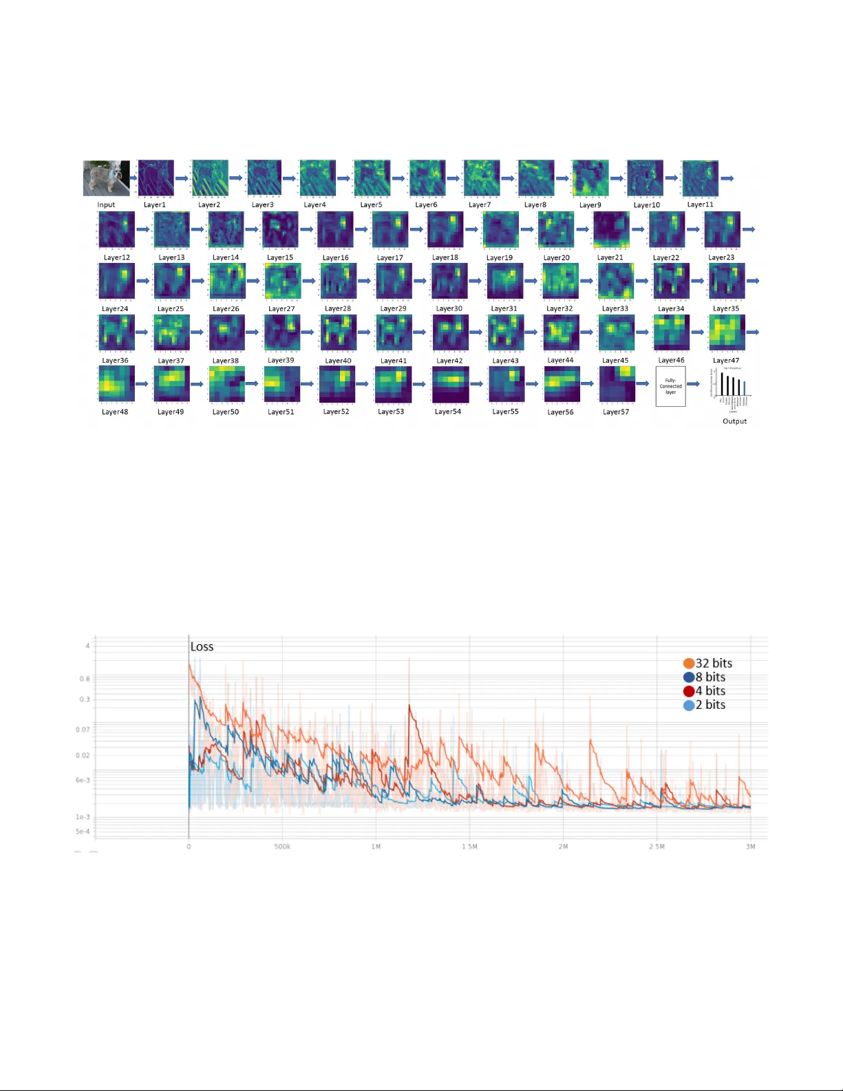
T emporal-Coded Deep Spiking Neural Network with Easy T raining and Robust P erf ormance Shibo Zhou, 1 Xiaohua Li, 1 Y ing Chen, 2 Sanjeev T . Chandrasekaran, 3 Arindam Sanyal 3 1 Dept. of ECE, Binghamton Univ ersity , Binghamton, NY , USA 2 (Corresponding Author) Harbin Institute of T echnology , China 3 Dept. of EE, Univ ersity at Buf falo, Buf falo, NY , USA { szhou19, xli } @binghamton.edu, yingchen@hit.edu.cn, { stannirk, arindams } @buf f alo.edu Abstract Spiking neural network (SNN) is promising b ut the dev el- opment has fallen far behind con ventional deep neural net- works (DNNs) because of difficult training. T o resolve the training problem, we analyze the closed-form input-output re- sponse of spiking neurons and use the response expression to build abstract SNN models for training. This av oids calculat- ing membrane potential during training and makes the direct training of SNN as efficient as DNN. W e show that the non- leaky integrate-and-fire neuron with single-spike temporal- coding is the best choice for direct-train deep SNNs. W e dev elop an energy-ef ficient phase-domain signal processing circuit for the neuron and propose a direct-train deep SNN framew ork. Thanks to easy training, we train deep SNNs under weight quantizations to study their robustness o ver low-cost neuromorphic hardware. Experiments show that our direct-train deep SNNs hav e the highest CIF AR-10 classifica- tion accuracy among SNNs, achieve ImageNet classification accuracy within 1% of the DNN of equiv alent architecture, and are robust to weight quantization and noise perturbation. 1 Introduction Spiking neural network (SNN) is interesting theoretically due to its strong bio-plausibility and practically because of its outstanding energy ef ficienc y . Neurons communi- cate via spikes just as biological neurons. They work asyn- chronously , i.e., generate output spikes without waiting for all input neurons to spike. This leads to advantages such as spike sparsity , low latency , and high energy efficienc y that are attracti v e for practical applications (Pfeiffer and Pfeil 2018; T av anaei et al. 2019). The performance of SNNs has fallen far behind conv en- tional deep neural networks (DNNs). One of the primary reasons is that SNNs are difficult to train. DNNs are for- mulated with the standard layer response y = f ( xW + b ) where gradient backpropagation can be efficiently con- ducted. In contrast, for SNNs we hav e to simulate the temporal-domain neuron membrane potentials with non- differentiable spik es. Gradient ev aluation is both difficult and time-consuming. Direct training of SNN has so far been limited to shallow networks only . No one has trained directly the SNNs on large datasets such as ImageNet. Copyright © 2021, Association for the Advancement of Artificial Intelligence (www .aaai.org). All rights reserved. SNNs are targeting neuromorphic hardware implementa- tions. Their robustness on low-cost neuromorphic hardware with limited memory , high noise, and large parameter drift- ing is critical for them to be competiti ve to DNNs in practical applications. This special yet important problem has been largely open. In this paper , we resolve the difficult training problem by developing a direct-train framework that does not need calculating neuron membrane potentials. W e address the ro- bustness problem by de v eloping a neuron circuit to e v aluate timing jitter and by training deep SNNs under weight quan- tizations. Our major contributions are listed as follo ws. • Closed-form analytical input-output responses of spik- ing neurons are studied systematically , which shows that the nonleaky integrate-and-fire neuron with single-spike temporal-coding is the best choice for direct-train SNNs. • Deep SNNs such as SpikingVGG16 and Spiking- GoogleNet are developed and trained over the CIF AR-10 and ImageNet datasets. New benchmark results are ob- tained. T o the best of our knowledge, this is the first time that direct-train SNN is reported for ImageNet. • A phase-domain signal processing neuron circuit is de- signed to sho w that our neuron is more energy-ef ficient than others and is robust to input timing jitter and weight quantization. Besides, our deep SNNs are trained under weight quantization and noise perturbation to demonstrate their robustness. This paper is organized as follows. Related works are in- troduced in Section 2. Spiking neurons and deep SNNs are described in Section 3. Experiments are presented in Section 4. Conclusions are giv en in Section 5. 2 Related W orks SNN training methods can be cate gorized into three classes: unsupervised learning, supervised learning with indirect training, and supervised learning with direct training (Pfeif- fer and Pfeil 2018). F or unsupervised learning, spike timing- dependent plasticity (STDP) is well kno wn (Caporale and Dan 2008; Diehl and Cook 2015; Kheradpisheh et al. 2018; Lee et al. 2018). Ne vertheless, the dependency on the local neuronal activities without a global supervisor makes it ha ve low performance in deep netw orks. For the second class, the popular approach is to translate pre-trained DNNs to SNNs (T av anaei et al. 2019). This can be conducted by mapping DNN neuron values to SNN neu- ron spike rates (Diehl et al. 2015; Rueckauer et al. 2017; Sengupta et al. 2019) or spike times (Zhang et al. 2019). Although the translation approach has had the best perfor- mance among SNNs so far , it unfortunately sacrifices im- portant SNN advantages such as spike sparsity and asyn- chronous processing, which degrades energy ef ficiency . Be- sides, many DNN techniques such as max-pooling and tanh activ ation are hard or inef ficient to cop y to SNN. Among the third class, SpikeProp (Bohte, K ok, and La Poutre 2002) minimized the loss between the true and de- sired spike times with gradient descent rule ov er soft nonlin- earity models. Gardner et al. (Gardner , Sporea, and Gr ¨ uning 2015) applied a probability neuron model to calculate gradi- ents. Gradient backpropagation was applied in (Hunsberger and Eliasmith 2016; Lee, Delbruck, and Pfeiffer 2016; Jin, Zhang, and Li 2018; W u et al. 2019b) based on spike rate coding where gradient backpropagation through both SNN layer responses and neuron membrane potential dynamics was needed, which made the algorithms extremely complex. Backpropagation through SNN layer responses only was ap- plied in (Mostafa 2017). Zhou and Li (Zhou and Li 2020) pointed out that the overly-nonlinear neuron response led to lo w training performance in SNNs. Existing direct train- ing approaches still fall short of efficienc y to deal with lar ge datasets such as ImageNet. A list of neuromorphic hardware has been developed for SNN, such as IBM T rueNorth (Merolla et al. 2014), Intel Loihi (Da vies et al. 2018), and BrainScaleS (Aamir et al. 2018b). F or ener gy efficiency , Hunsberger and Eliasmith (Hunsberger and Eliasmith 2016) estimated that a synaptic operation consumed only 8% of the energy of a micropro- cessor floating-point operation. Cao et al. (Cao, Chen, and Khosla 2015) showed that SNN implemented in a neuromor- phic circuit with 45 pJ per spike was 185 times more ener gy- efficient than the FPGA-based DNN implementation. W ith 26 pJ per spike, IBM T rueNorth consumed 1 . 76 × 10 5 times less energy than computer simulations ov er microproces- sors, and 769 times less energy than microprocessor-based neuromorphic hardware. Zhou et al. (Zhou et al. 2020) de- veloped an analog neuron circuit with 19 pJ per spike, with which SNN-based YO YOv2 consumed only 0.247 mJ for detecting objects in an image frame. Neuromorphic hardware has the problem of noise, param- eter drifting, as well as severe limitation on resources such as memory . Implementing SNNs in neuromorphic hardware without rob ustness optimization sho wed hea vy performance degradation (Esser et al. 2016; G ¨ oltz et al. 2019). Rathi et al. (Rathi, Panda, and Roy 2018) studied the pruning of unimportant weights and quantizing important weights to improv e energy ef ficienc y , but for shallo w SNNs only . 3 Deep SNN with Easy and Direct T raining The major hurdle to training SNNs is that ev ery neuron’ s membrane potential has to be calculated in each training it- eration. This is not a problem when implementing SNNs in neuromorphic hardware but is computationally prohibitiv e Figure 1: Integrate-and-fire spiking neuron model. for software implementation and gradient-based training. Non-differential spike wav eform is the second hurdle. Our objectiv e is to completely av oid the calculation of membrane potential and spike wav eform during training. Instead, we train the SNNs based on an abstract layer r esponse model of the neurons. As illustrated in Fig. 1, the left figure is the spiking neuron model for real hardw are implementation and inference only , where the weights w j i need to be learned. The right figure is its layer response model, where we use the closed-form input-output response t j = f ( t i , w j i ) to train the weights w j i . Since the weights of the two figures are identical, the weights trained in the right figure are di- rectly used to implement the SNN in the left figure. In this section, we first sho w that only a special spiking neuron is appropriate for such direct training. Then, we show that this spiking neuron can be practically realized in energy- efficient hardware. Finally , based on this neuron, we propose a direct-train framew ork for deep SNNs. 3.1 Layer Response Models of Spiking Neur ons For the neuron illustrated in Fig. 1 (left), we consider the integrated-and-fire model. Membrane potential v j ( t ) of the neuron j is modeled as dv j ( t ) dt + bv j ( t ) = X i w j i X k g ( t − t ik ) , (1) where b is a positi ve constant representing the leaky rate of the membrane potential, w j i is the weight of the synaptic connection from the input neuron i to the output neuron j , g ( t ) is the synaptic current kernel function or spike wa ve- form, and t ik is the spiking time of the k th spike of the i th in- put (pre-synaptic) neuron. b > 0 means leaky inte grate-and- fir e (LIF) neuron, while b = 0 means nonleaky inte grate- and-fir e (IF) neuron. Once v j ( t ) reaches spiking threshold θ , the neuron generates an output (post-synaptic) spike and the membrane potential is reset. Information can be encoded in spike rate r j , spike time t j , or other means. W e consider the first two, which we call rate coding and temporal coding, respecti vely . Rate r j is the av erage spike rate from t = 0 to t = T . For temporal coding, each neuron generates a single spike during the time period T . W e denote the spik e time as t j and adopt the time-to-first- spike (TTFS) code (G ¨ oltz et al. 2019). W e hav e conducted a thorough study of the solutions to (1) in order to find desirable layer response models. Details are in T echnical Appendix A. W e analyze our major obser- vations only in this subsection. Consider rate coding first. W ith impulse spike g ( t ) = δ ( t ) , nonleaky IF neuron has closed-form layer response r j = ReLU X i r i w j i θ ! , (2) where ReLU( x ) = max { 0 , x } . See (18) for deriv ations. Similar expressions exist for Heaviside and exponentially- decaying spike wa veforms (21)(23). Since these expressions are identical to DNN’ s layer response, we can directly train a network implemented in software based on (2) and apply the resulted weights w j i to the real SNN implemented in neuromorphic hardware. Note that (2) is also the theoretical basis for translat- ing DNNs to SNNs (Cao, Chen, and Khosla 2015; Diehl et al. 2015). It is interesting to see that direct-train SNN and translate-SNN become similar based on (2). The only dif- ference is that the latter trains weights w j i /θ instead of w j i and thus needs weight normalization. Unfortunately , (2) is an approximate model only . Modeling error accumulates to the detrimental level in deep SNNs (Rueckauer et al. 2017). Corrections are developed for translate-SNNs to mitigate the error to some extent. The corrections need to calculate mem- brane potential, which makes direct-train dif ficult again. For rate-coded LIF neurons, layer responses become nu- merically unstable for training. As sho wn in (25), LIF neu- ron with the impulse spike wa v eform has layer response r j = ReLU( − b log − 1 (1 − θ / X i w j i / ( e b/r i − 1))) . (3) Random weights w j i often make log function undefined, which means training can not proceed. The same problem happens for other spike wa v eforms (28)(30). Next, for temporal coding, similar numerical instability happens for LIF neurons with the exponentially-decaying spike wav eform. As sho wn in (42) and (44), the layer re- sponses are expressed in either Lambert W function or quadratic equation roots. Random weights often result in negati v e or complex v alues that pre vent gradient updating. Fortunately , temporal-coded nonleaky IF neurons have layer responses desirable for direct training. W ith the exponentially-decaying spike wav eform, the layer response can be formulated as (Mostafa 2017) e t j τ = X i ∈C e t i τ w j i P ` ∈C w j ` − θ (4) where the set C = {∀ k : t k < t j } . See (35) for deriv ations. W ith the Heaviside spike wa veform, both IF and LIF neu- rons hav e similar layer responses, see (33) and (38). There is no significant modeling error and the expressions have nice numerical stability . Since the ener gy ef ficienc y of SNNs depends on the num- ber of spikes, we prefer single-spike neurons. Therefore, the best choice is to adopt the single-spike temporal-coded non- leaky IF neuron to implement SNNs and train them based on (4). Note that we prefer the exponentially-decaying spike wa veform rather than the Heaviside spike wa v eform because the former can be truncated to short spike duration in prac- tice to enhance energy ef ficienc y . 3.2 Circuit of T emporal-Coded Spiking Neuron Most existing neuron circuits are designed for rate coding or for generating special spike patterns (Aamir et al. 2018a). Few circuits are reported for single-spike neurons. There- fore, we present a ne w neuron circuit design to show that the single-spike temporal-coded neuron with exponentially- decaying spike wa veform can be realized practically . This circuit will also help us study energy ef ficiency , timing jit- ter , and weight quantization rob ustness. For neuron circuit designs, prior works hav e used ana- log voltage domain (VD) signal processing to realize LIF neurons using CMOS circuits (Indiv eri 2003; W ijek oon and Dudek 2009; W u et al. 2015). VD signal processing tech- niques require high-gain amplifiers which are energy inef fi- cient to design in advanced CMOS nodes with lo w intrinsic gain. T o reduce energy consumption, we introduce phase- domain (PD) signal processing into SNN design. PD signal processing con verts VD signal excursions into phase domain for further processing, and has well documented advantages ov er VD processing such as higher energy ef ficiency , abil- ity to better lev erage CMOS technology scaling and simpler circuit design. While PD signal processing has been widely adopted in the circuit design community for high energy- efficienc y data-conv erter design (Sanyal et al. 2014; Sanyal and Sun 2016; Jayaraj et al. 2019a,b), a key contribution of this work is the introduction of PD signal processing to SNN design field for the first time. Fig. 2 shows the circuit schematic of the IF neuron de- signed with voltage-controlled ring oscillator (VCO) based integrators. As shown in Fig. 2(a), if a voltage input V in ( t ) is applied to a ring VCO, its instantaneous phase is gi v en by Φ( t ) = R 2 π k v co V in ( t ) dt , where k v co is VCO tuning gain. Thus, a VCO acts as a perfect PD integrator with infinite dc gain (San yal and Sun 2016; T aylor and Galton 2010; Perrott et al. 2008), and is perfectly positioned to realize non-leaky integration. While the VCO phase is integral of its input, the phase output cannot be directly extracted. Rather, the volt- age output of one of the in verters is read out which acts as a pulse-width modulated signal (PWM) and encodes the phase information in the width of its pulses as sho wn in Fig. 2(a). The ring VCO has a highly digital architecture and can oper - ate from very lo w supply v oltages. Hence, VCO can be used as an integrator in advanced CMOS processes which allows area and power scaling unlik e VD integrators. Fig. 2(b) shows the schematic of the proposed phase- domain IF neuron designed using VCOs, in which VCO1 and VCO3 act as global reference sources driv en by con- stant inputs and are shared with all the neurons. T 1 and T 2 represent 2 inputs to the neuron while the resistors R 1 j and R 2 j denote the weights of synaptic connections of the in- puts to the neuron, respectiv ely . When the inputs to VCO2 spike, the output phase of the VCO2 jumps abruptly and VCO2 starts running at a high frequency . Outputs of VCO1 and VCO2 driv e two counters which increment at the ris- ing edge of VCO outputs. The difference between the two counters is used to driv e VCO2 through negativ e feedback. The negati ve feedback loop forces VCO2 to track VCO1, and the frequency of VCO2 starts decaying exponentially till it reaches the frequency of VCO1 as shown in Fig. 2(b). 1.9 2 2.1 2.2 2.3 2.4 0 0.5 1 1.9 2 2.1 2.2 2.3 2.4 0 0.5 1 1.9 2 2.1 2.2 2.3 2.4 0 0.5 1 T ime ( µs) T1 VCO2 VCO1 Figure 2: IF neuron circuit schematic using time-domain signal processing circuits. (a) Operation of ring-inv erter -based VCO. (b) Circuit schematic of 1 neuron designed using ring VCOs. W aveforms of input, output and intermediate nodes sho w that T 1 generates an input spike ev ery microsecond, VCO1/VCO2 reshape the spike into the exponentially-decaying spike wav eform, and VCO3/VCO4 generate an output spike e very tw o microseconds. Thus, VCO2 realizes the exponential decaying synaptic ker - nel. The frequency difference between VCO1 and VCO2 is extracted using an XOR gate and sent to VCO4 for accumu- lation. VCO4 switches between two frequencies depending on whether the XOR output is high or low . Similar to VCO1 and VCO2, VCO3 and VCO4 also dri v e two counters at ris- ing edges of their respective outputs. Once the dif ference between the two counter outputs exceeds a threshold v alue, an output spike is generated, and both the counters are reset. The proposed circuit is highly scalable since it is built using digital CMOS circuits. The synaptic weights can be made tunable by using a digitally controllable resistor bank. The neuron consumes less than 10 pJ/spike in 65 nm process and the energy consumption will reduce further with tech- nology scaling. This leads to an energy efficienc y gain of 45% o ver (Zhou et al. 2020). 3.3 Direct-T rain Framew ork f or Deep SNNs For training, we implement the abstract SNNs in software based on (4). Specifically , in the ` th layer , z ` − 1 ,i = e t ` − 1 ,i /τ and z `,j = e t `,j /τ are used directly as neuron’ s input and output. For an L -layer deep SNN, define the input as z 0 with elements z 0 ,i and the final output as z L with elements z L,i . Smaller z L,i means stronger classification output. Then we hav e z L = f ( z 0 ; w ) with nonlinear mapping f and trainable weight w which includes all weights w ` j i . Let the targeting output be class c . W e train the network with the loss function L ( z L , c ) = − log z − 1 L,c P i 6 = c z − 1 L,i + K L X ` =1 X j max ( 0 , θ − X i w ` j i ) + λ L X ` =1 X j,i ( w ` j i ) 2 . (5) The first term is to mak e z L,c the smallest (equi v alently t L,c the smallest) one. The second term is the weight sum cost, which enlarges each neuron’ s input weight summation to in- crease its firing probability . The third term is L 2 regulariza- tion to prevent weights from becoming too large. The pa- rameters K and λ are weighting coefficients. Thanks to the closed-form expression (4), gradient backpropagation can be used to train the weights. The training becomes nothing dif- ferent from con v entional DNNs. Equations (4) and (5) were initially given in (Mostafa 2017). Howe ver , only shallow networks with 2 ∼ 3 fully- connected layers were tried and the performance was lo w . One of the problems of the algorithm presented in (Mostafa 2017) is that t j > t i for i ∈ C was not checked, which led to t j ≤ t i or ev en negati v e timing that was not hardware realizable. Another problem is that the algorithm is not suit- able for deep SNN. As a result, this work did not arouse too much interest and the research progress has been slow . W e have resolved these problems by dev eloping the fol- lowing new algorithm to calculate (4): 1) Use the SOR T function to sort inputs e t i /τ ; 2) Use the CUMSUM function to list all possible P i ∈C w j i and P i ∈C w j i e t i /τ ; 3) Calcu- late e t j /τ for each element in the list; 4) Find the first one that satisfies e t j /τ > e t i /τ for i ∈ C and e t j /τ ≤ e t i /τ for i 6∈ C . Refer to our source code for details. This algorithm is much easier to implement and more efficient to run for deep SNNs. Note that real hardw are SNN does not need this algorithm because spike time is naturally ordered. As long as P i w j i > θ , our algorithm can alw ays provide hardware-compatible solutions e t j /τ . With some heuristic con v ergence improving techniques (see experiment section), we hav e improved greatly both computation speed and con- ver gence, which makes it possible to train deep SNNs. T o design deep SNNs, it is helpful to follo w DNN ar - chitectures so as to exploit the extensi v e DNN research experience. For this we need to study ho w some DNN- specific techniques can be realized in SNNs, such as pooling, batch normalization (BN), and local response normalization (LRN). This issue has nev er been addressed in direct-train SNN including (Mostafa 2017). For max-pooling, in software SNN training we have e t j /τ = min i e t i /τ . In real SNN hardware this can be re- alized as Fig. 1 using a lar ge enough w j i , which lets the first arriv al spike activ ate the output spike. A verage-pooling can be realized by letting w j i = θ / ( N − 1) for N inputs. For BN, in software abstract SNN we need to calculate e t j /τ = γ /σ ( e t i /τ − µ ) + β , where γ , σ, µ, β are parameters obtained from training. Rewriting it as e t j /τ = e ( t i + τ log γ /σ ) /τ + e log( β − γ µ/σ ) , (6) it is easy to see that (6) can be realized in SNN hardware with two input neurons: one has spike time t i with a con- stant delay τ log γ /σ , and the other has a constant spike time τ log ( β − γ µ/σ ) . The weight should be w j i = θ . Note that spike time delay is a standard feature in SNN hardw are such as IBM T rueNorth. For LRN, the implementation is similar to BN but is much more complex. W e also need to exploit the asynchronous property of SNN, i.e., reference timing t = 0 of a layer can be shifted to some non-zero value. In softw are SNN we hav e e t j /τ = e t i /τ / ( γ + α P ` e 2 t ` /τ ) β for constants γ , α and β . In hardware, we can use a neuron to calculate P ` e 2 t ` /τ as av erage-pooling and then use another set of neurons to realize the rest operations similar to BN. The above DNN-adaptation techniques would make our direct-train SNN look similar to translate-SNN. This is not surprising as our abstract SNN is designed to be trained sim- ilarly as DNN. The major differences are, first, we directly train the real SNN weights w j i and thus do not need com- plex weight normalization or SNN structure change. Sec- ond, we hav e the flexibility to impro ve DNN techniques and train them to fit with SNN. For example, in BN, we can train SNN to guarantee the output in (6) be non-negati v e. Third, we can dev elop SNN specific techniques to outper- form DNNs, such as adjusting θ in (5) to promote sparsity and energy efficienc y . Note that besides spike sparsity , our temporal-coded SNN has neuron sparsity , i.e., only neurons in C need to spike. Translate-SNN does not have such spar- sity . The sparsity of translate-SNN usually means to reduce the number of spikes by using a shorter T , which makes the SNN work in transient response mode and thus suffer from performance degradation. 4 Experiments In this section, we report our experiments over three stan- dard datasets: MNIST , CIF AR-10, and ImageNet 1 . W e de- signed three deep SNN models, which are sho wn in T able 1, and ev aluated their accurac y and rob ustness. 1 Our source code can be found at https://github .com/ zbs881314/T emporal- Coded- Deep- SNN 4.1 Classification Accuracy MNIST : The MNIST image pixels were normalized to p i ∈ [0 , 1] and encoded into spiking time t i = α ( − p i + 1) . The parameter α was used to adjust spike temporal separa- tion. W e trained the network for 50 epochs with batch size 10 using the Adam optimizer . The learning rate started at 0 . 001 and gradually reduced to 0 . 0001 at the last epoch, with learning decay lr decay = (learning end -learning start)/50. W e set K = 100 and λ = 0 . 001 . According to (4), gradients could become very large in case P ` w j ` is near θ , which is harmful to training. Therefore, we limited the maximum allowed row-normalized Frobenius norm of the gradient of each weight matrix to 10 . W e trained this network with noisy input spike times. Classification accuracy is shown in T able 2. The proposed network had the highest accuracy (99.33%) among the SNNs listed in the table, yet had the smallest network size with the least number of trainable weights (21K). Because of the asynchronous operation of our SNN, on average 94% neurons spiked, which led to sparsity 0.94. The total con- sumed energy of the proposed network w as 205 nJ assuming each spike cost 10 pJ based on the proposed neuron circuit and sparsity 0.94. CIF AR-10: Our SNN model for CIF AR-10 was dev eloped based on the VGG16 model (Liu and Deng 2015; Simon yan and Zisserman 2014), hence called SpikingVGG16. T o en- code image pixels to spike time, we applied encoding rule t i = αp i and used a relati vely lar ge α to enlarge spike time separation so that all pixel values could potentially be used. W e e xploited data augmentation such as crop, flip, and whiten to increase the diversity of data av ailable for training. The learning rate started at 0.01 and ended at 0.0001. W e ran 320 epochs and after 240 epochs the training tended to con- ver ge. The batch size was 128. The other hyper-parameters were the same as the MNIST experiments. As shown in T able 2, the testing accuracy of our Spik- ingVGG16 set a new record at 92.68%, higher than all the listed SNNs including the state-of-the-art of (W u et al. 2019b). Especially , our model had higher accuracy than the CNN-based VGG16 (Liu and Deng 2015). Our network en- joyed a sparsity of 0 . 62 which means only 62% neurons sent spikes. It consumed 0 . 336 mJ of energy for each image in- ference. ImageNet: W e built our deep SNN model based on the popular GoogleNet architecture (Szegedy et al. 2015), hence called SpikingGoogleNet. W e simply replaced CNN layers with SCNN layers and FC layers with spiking FC layers. W e used 1.2 million images to train the network. Training parameters were similar to the CIF AR-10 experiments, and the training procedure followed that of GoogleNet. The in- put image was 224 × 224 × 3 and was randomly cropped from a resized image using the scale and aspect ratio augmenta- tion. W e used SGD with a batch size of 256, learning rate decay 0.0001, and momentum 0.9. W e started from a learn- ing rate of 0.1 and divided it by 10 three times. When the MNIST SCNN(5,32,2) → SCNN(5,16,2) → FC(10) CIF AR-10 SpikingV GG16 : SCNN(3,64,1) → SCNN(3,64,1) → MP(2) → SCNN(3,128,1) → SCNN(3,128,1) → MP(2) → SCNN(3,256,1) → SCNN(3,256,1) → SCNN(3,256,1) → MP(2) → SCNN(3,512,1) → SCNN(3,512,1) → SCNN(3,512,1) → MP(2) → SCNN(3,1024,1) → SCNN(3,1024,1) → SCNN(3,1024,1) → MP(2) → FC(4096) → FC(4096) → FC(512) → FC(10) ImageNet SpikingGoogleNet : replace GoogleNet CNN/FC layers with SCNN/FC layers T able 1: Proposed models. SCNN(5,32,2) means spiking CNN layer with 32 5 × 5 kernels and stride 2. FC(10) means fully- connected layer with 10 output neurons. MP(2) means 2 × 2 max-pooling layer . τ = θ = 1 . Bias is added as t 0 = 0 . Dataset Models Method Accuracy W eights(million) Sparsity (Ciresan et al. 2011) CNN 99.73% 0.069 no (Kheradpisheh et al. 2018) SNN+STDP 98.40% 0.076 no (Lee et al. 2018) SNN+STDP 91.10% 0.025 no MNIST (Mostafa 2017) SNN+DT 97.55% 0.635 0.51 (Zhang et al. 2019) SNN+tran 99.08% 3.9 no (W u et al. 2019a) SNN+DT 99.26% 0.051 no Our Model SNN+DT 99.33% 0.021 0.94 (Liu and Deng 2015) (VGG16) CNN 91.55% 15 no (Hunsberger and Eliasmith 2016) SNN+tran 82.95% 39 no CIF AR-10 (Rueckauer et al. 2017) SNN+tran 90.85% 62 no (Sengupta et al. 2019) (VGG16) SNN+tran 91.55% 15+ no (W u et al. 2019b) SNN+DT 90.53% 45 no Our Model SNN+DT 92.68% 54 0.62 (Simonyan and Zisserman 2014) (V GG16) CNN 71.5% 138 no (Szegedy et al. 2015) (GoogleNet) CNN 69.8% 6.8 no ImageNet (Rueckauer et al. 2017) (VGG16) SNN+tran 49.61% 138 no (Sengupta et al. 2019) (VGG16) SNN+tran 69.96% 138+ no (Zhang et al. 2019) (VGG16) SNN+tran 70.87% 138+ no Our Model SNN+DT 68.8% 6.8 0.56 T able 2: Classification accuracy comparison. DT : direct training. tran: translate SNN. training error was no longer reducing, retraining and fine- tuning with very small learning rates were conducted until the test accuracy no longer increased. Results of T op-1 testing accuracy are sho wn in T able 2. Our SpikingGoogleNet achieved 68.8% accuracy , only 1.0% lower than the CNN-based GoogleNet. VGG16-based SNNs had slightly better performance because CNN-based VGG16 had better accuracy than GoogleNet. But they had much larger netw ork sizes. For energy consumption, our network enjoyed a sparsity of 0 . 56 which means only 56% of neurons were activ ated during image inference. The total energy consumption was thus 0 . 038 mJ. For the translate-SNN model (Sengupta et al. 2019), if implemented in IBM T rueNorth with 26 pJ per spike and having an av erage of 256 spikes per neuron with rate coding, each of them would consume 900 mJ, sev eral orders bigger than ours. T o the best of our knowledge, fe w works were reported ov er the CIF AR-10 dataset using direct training SNN (ex- cept (W u et al. 2019b)) and none was reported ov er the Im- ageNet dataset. Our models hence set up new benchmark accuracy in both cases. There is still a big gap between SNN and DNN (T an and Le 2019). Ne vertheless, our e xperiments showed that our proposed SNNs could achieve similar ac- curacy as the DNNs with similar netw ork size and archi- tecture. This fact was also demonstrated in many translate SNN works. W e expect that SNN performance could catch up rapidly after the training hurdle is resolved. 4.2 Robustness Neuron Robustness: For neuromorphic circuits, a prob- lem is that they are very sensitiv e to changes in operating conditions such as supply voltage or temperature. In Fig. 2, we hav e used differential architecture in which VCO phase is always compared with phase from a reference VCO rather than using the absolute phase from a single VCO. While this architectural choice doubles area and energy consumption, it also increases robustness to changes in operating conditions. For temporal-coded neurons, an important distortion mea- sure is spike timing jitter , which is defined as | t measured j − t desired j | /t desired j . F or mixed digital-analog circuits, there are quantization noise and circuit noise, which we simply com- bine into synaptic weight quantization noise. W e conducted circuit simulation under various input timing jitters and weight quantizations, and the results are summarized in T a- ble 3. Both input jitter and quantization of synaptic weights change the temporal location of the output spikes. As the input jitter was swept from 1% to 9%, the output jitter var - Input Output Quantization Output Jitter (%) Jitter (%) Lev el Jitter (%) 1 0.024 4-bit 0.957 3 0.189 8-bit 0.268 5 0.397 16-bit 0.008 7 0.789 24-bit 0.004 9 0.997 32-bit 0.004 T able 3: Jitter in output spike v ersus input jitter and synaptic weight quantization. ied from 0.024% to 0.997% only . Such a good inherent jit- ter suppression capability was due to the phase-locked loop (PLL) which low-pass-filtered input jitter . Quantizing synaptic weights (for 2-input case) increased output jitter from 0.004% in the case of 32-bit quantization to 0.957% in the case of 4-bit quantization. Coarse quanti- zation thus led to large jitter . One of the reasons was that in our neuron model (4) the denominator P ` w j ` − θ could be small and a slight change of weights w j ` might cause a big change in t j . T o mitigate this problem, we can set θ in (5) to a bigger number during training. Examining the numbers in T able 3 more carefully , we see that 4-bit quantization, which has quantization SNR (signal to noise ratio) 6 . 02 × 4 ≈ 24 dB, led to output jitter of 0.957% which means SNR 20 log 10 (1 /. 00957) ≈ 40 dB. A 40 dB SNR means that the neuron was extremely robust to weight quantization. Deep SNN Robustness: T o ev aluate the robustness of deep SNNs, we experimented with both weight quantiza- tion and noise perturbation. For weight quantization, the weights were quantized to 32-bit, 8-bit, 4-bit, and 2-bit words. Thanks to our easy training models, we could re- train the deep SNNs simply follo wing the procedure de vel- oped for conv entional CNN quantization (Li, Zhang, and Liu 2016; Rasteg ari et al. 2016). Specifically , the forward inference used quantized weights while the backward gradi- ent propagation used full-precision weights. W e first trained with 32-bit quantization. After the training conv er ged, we applied 8-bit quantization and retrain the SNNs. This proce- dure was repeated until the 2-bit quantization. T able 4 shows the testing accuracy under weight quan- tization. For the models over MNIST , CIF AR10 and Ima- geNet, weight quantization caused the worst accurac y loss of 0 . 22% , 1 . 75% , and 8 . 8% , respectiv ely . As comparison, we listed two typical CNN weight quantization results (Cheng et al. 2018; Zhang et al. 2018), which indicated a similar per- formance degradation pace. The results demonstrated that the SNN models were robust to weight quantization for rel- ativ ely small datasets and small netw orks. For larger net- works, the weights would better be encoded in 4-bit or o ver . T o ev aluate noise perturbation, we added random noise to the trained weights. Experiment results are shown in Fig. 3, together with the results of weight quantization in T able 4 (expressed in SNR). W e find that 24dB quantization noise (4-bit quantization) reduced ImageNet classification accu- racy to 65.2%. Noise at 24dB SNR reduced ImageNet clas- Model Bits MNIST CIF AR-10 ImageNet 32 99.33% 92.68% 68.8% Our 8 99.32% 91.87% 66.1% Models 4 99.21% 91.38% 65.2% 2 99.11% 90.93% 60.0% (Cheng et al. 32 98.66% 84.80% - 2018) 8 98.48% 84.07% - 2 96.34% 81.56% - (Zhang et al. 32 - 92.1% 70.3% 2018) 4 - - 70.0% 2 - 91.8% 68.0% T able 4: Accuracy versus weight quantization. Figure 3: Accuracy versus weight quantization (Q) and noise perturbation (N). Dashed Lines: baseline (32-bit quantiza- tion and noiseless cases). Note: 8,4,2-bit quantizations cor- respond to quantization SNRs 48, 24, 12dB, respectiv ely . sification accuracy to 65.43%. Both cases had a small 3.5% performance loss only . Because T able 3 indicated that neuron noise (explained as jitter) was usually very small, we just need to pay attention to high SNR scenarios, such as 24dB and above (corresponding to 4-bit or above quantization). In this case, the accuracy reduction was negligible. Therefore, the deep SNNs were robust to both weight quantization and noise perturbation. Extra experiment results are in T echnical Appendix B. 5 Conclusion In this paper , we dev elop direct-train deep SNNs that can be easily trained over large datasets such as ImageNet. W e show that our SNNs can realize classification accuracy within 1% of (or e v en better than) DNNs of similar size and architecture. A circuit schematic of the adopted neuron is de- signed with phase-domain signal processing, which sho ws 45% energy ef ficienc y gain o ver the e xisting state of the art. Both the neuron and the deep SNNs are demonstrated as robust to timing jitter , weight quantization, and noise. The easy training, high performance, and robustness indicate that SNNs can be competiti ve to DNNs in practical applications. References Aamir , S. A.; M ¨ uller , P .; Kiene, G.; Kriener, L.; Stradmann, Y .; Gr ¨ ubl, A.; Schemmel, J.; and Meier , K. 2018a. A mixed- signal structured adex neuron for accelerated neuromorphic cores. IEEE tr ansactions on biomedical cir cuits and systems 12(5): 1027–1037. Aamir , S. A.; Stradmann, Y .; M ¨ uller , P .; Pehle, C.; Hartel, A.; Gr ¨ ubl, A.; Schemmel, J.; and Meier, K. 2018b. An ac- celerated lif neuronal network array for a lar ge-scale mix ed- signal neuromorphic architecture. IEEE T ransactions on Cir cuits and Systems I: Re gular P apers 65(12): 4299–4312. Bohte, S. M.; K ok, J. N.; and La Poutre, H. 2002. Error- backpropagation in temporally encoded networks of spiking neurons. Neur ocomputing 48(1-4): 17–37. Cao, Y .; Chen, Y .; and Khosla, D. 2015. Spiking deep con- volutional neural networks for ener gy-ef ficient object recog- nition. International Journal of Computer V ision 113(1): 54–66. Caporale, N.; and Dan, Y . 2008. Spike timing–dependent plasticity: a Hebbian learning rule. Annu. Rev . Neur osci. 31: 25–46. Cheng, H.-P .; Huang, Y .; Guo, X.; Huang, Y .; Y an, F .; Li, H.; and Chen, Y . 2018. Dif ferentiable fine-grained quanti- zation for deep neural network compression. arXiv pr eprint arXiv:1810.10351 . Ciresan, D. C.; Meier , U.; Gambardella, L. M.; and Schmid- huber , J. 2011. Con volutional neural network committees for handwritten character classification. In 2011 Interna- tional Confer ence on Document Analysis and Recognition , 1135–1139. IEEE. Davies, M.; Sriniv asa, N.; Lin, T .-H.; Chinya, G.; Cao, Y .; Choday , S. H.; Dimou, G.; Joshi, P .; Imam, N.; Jain, S.; et al. 2018. Loihi: A neuromorphic manycore processor with on- chip learning. IEEE Micr o 38(1): 82–99. Diehl, P . U.; and Cook, M. 2015. Unsupervised learning of digit recognition using spike-timing-dependent plasticity . F rontier s in computational neur oscience 9: 99. Diehl, P . U.; Neil, D.; Binas, J.; Cook, M.; Liu, S.-C.; and Pfeiffer , M. 2015. Fast-classifying, high-accuracy spiking deep networks through weight and threshold balancing. In 2015 International J oint Confer ence on Neural Networks (IJCNN) , 1–8. ieee. Esser , S.; Merolla, P .; Arthur , J.; Cassidy , A.; Appuswamy , R.; Andreopoulos, A.; Berg, D.; McKinstry , J.; Melano, T .; Barch, D.; et al. 2016. Con v olutional Networks for Fast, Energy-E cient Neuromorphic Computing. CoRR abs/.().: http://arxiv . or g/abs/1603.08270 . Gardner , B.; Sporea, I.; and Gr ¨ uning, A. 2015. Learning spatiotemporally encoded pattern transformations in struc- tured spiking neural networks. Neur al computation 27(12): 2548–2586. G ¨ oltz, J.; Baumbach, A.; Billaudelle, S.; Breitwieser , O.; Dold, D.; Kriener, L.; Kungl, A. F .; Senn, W .; Schem- mel, J.; Meier , K.; et al. 2019. Fast and deep neuromor- phic learning with time-to-first-spike coding. arXiv pr eprint arXiv:1912.11443 . Hunsberger , E.; and Eliasmith, C. 2016. T raining spiking deep networks for neuromorphic hardware. arXiv preprint arXiv:1611.05141 . Indiv eri, G. 2003. A lo w-po wer adaptiv e integrate-and-fire neuron circuit. In IEEE International Symposium on Cir- cuits and Systems , volume 4, IV –IV . Jayaraj, A.; Danesh, M.; Chandrasekaran, S. T .; and Sanyal, A. 2019a. Highly Digital Second-Order ∆Σ VCO ADC. IEEE T ransactions on Circuits and Systems I: Regular P a- pers 66(7): 2415–2425. Jayaraj, A.; Das, A.; Arcot, S.; and Sanyal, A. 2019b. 8.6fJ/step VCO-Based CT 2nd-Order ∆Σ ADC. In IEEE Asian Solid-State Cir cuits Confer ence (A-SSCC) , 197–200. Jin, Y .; Zhang, W .; and Li, P . 2018. Hybrid macro/micro lev el backpropagation for training deep spiking neural net- works. In Advances in neural information pr ocessing sys- tems , 7005–7015. Kheradpisheh, S. R.; Ganjtabesh, M.; Thorpe, S. J.; and Masquelier , T . 2018. STDP-based spiking deep con volu- tional neural networks for object recognition. Neural Net- works 99: 56–67. Lee, C.; Sriniv asan, G.; Panda, P .; and Roy , K. 2018. Deep spiking con v olutional neural network trained with unsuper- vised spike-timing-dependent plasticity . IEEE T ransactions on Cognitive and Developmental Systems 11(3): 384–394. Lee, J. H.; Delbruck, T .; and Pfeiffer , M. 2016. T raining deep spiking neural networks using backpropagation. F r on- tiers in neur oscience 10: 508. Li, F .; Zhang, B.; and Liu, B. 2016. T ernary weight net- works. arXiv preprint arXiv:1605.04711 . Liu, S.; and Deng, W . 2015. V ery deep conv olutional neu- ral network based image classification using small training sample size. In 2015 3rd IAPR Asian confer ence on pattern r ecognition (A CPR) , 730–734. IEEE. Merolla, P . A.; Arthur , J. V .; Alvarez-Icaza, R.; Cassidy , A. S.; Sawada, J.; Akopyan, F .; Jackson, B. L.; Imam, N.; Guo, C.; Nakamura, Y .; et al. 2014. A million spiking- neuron inte grated circuit with a scalable communication net- work and interface. Science 345(6197): 668–673. Mostafa, H. 2017. Supervised learning based on temporal coding in spiking neural networks. IEEE transactions on neural networks and learning systems 29(7): 3227–3235. Perrott, M.; et al. 2008. A 12-bit 10-MHz bandwidth continuous-time ADC with a 5-bit 950-MS/s VCO-based quantizer . IEEE J. Solid-State Cir cuits . Pfeiffer , M.; and Pfeil, T . 2018. Deep learning with spiking neurons: opportunities and challenges. F r ontiers in neur o- science 12: 774. Rastegari, M.; Ordonez, V .; Redmon, J.; and Farhadi, A. 2016. Xnor-net: Imagenet classification using binary con vo- lutional neural networks. In Eur opean conference on com- puter vision , 525–542. Springer . Rathi, N.; Panda, P .; and Roy , K. 2018. STDP-based prun- ing of connections and weight quantization in spiking neural networks for energy-ef ficient recognition. IEEE T r ansac- tions on Computer-Aided Design of Inte grated Cir cuits and Systems 38(4): 668–677. Rueckauer , B.; Lungu, I.-A.; Hu, Y .; Pfeif fer , M.; and Liu, S.-C. 2017. Conv ersion of continuous-v alued deep networks to efficient event-dri v en networks for image classification. F rontier s in neur oscience 11: 682. Sanyal, A.; Ragab, K.; Chen, L.; V iswanathan, T .; Y an, S.; and Sun, N. 2014. A hybrid SAR-VCO ∆Σ ADC with first- order noise shaping. In IEEE Custom Inte grated Cir cuits Confer ence , 1–4. Sanyal, A.; and Sun, N. 2016. A 18.5-fJ/step VCO-based 0– 1 MASH ∆ − Σ ADC with digital background calibration. In 2016 IEEE Symposium on VLSI Circuits (VLSI-Cir cuits) , 1–2. IEEE. Sengupta, A.; Y e, Y .; W ang, R.; Liu, C.; and Roy , K. 2019. Going deeper in spiking neural networks: Vgg and residual architectures. F rontier s in neur oscience 13: 95. Simonyan, K.; and Zisserman, A. 2014. V ery deep con v o- lutional networks for large-scale image recognition. arXiv pr eprint arXiv:1409.1556 . Szegedy , C.; Liu, W .; Jia, Y .; Sermanet, P .; Reed, S.; Anguelov , D.; Erhan, D.; V anhoucke, V .; and Rabinovich, A. 2015. Going deeper with con volutions. In Pr oceedings of the IEEE conference on computer vision and pattern reco g- nition , 1–9. T an, M.; and Le, Q. V . 2019. Efficientnet: Rethinking model scaling for con v olutional neural networks. arXiv pr eprint arXiv:1905.11946 . T avanaei, A.; Ghodrati, M.; Kheradpisheh, S. R.; Masque- lier , T .; and Maida, A. 2019. Deep learning in spiking neural networks. Neural Networks 111: 47–63. T aylor, G.; and Galton, I. 2010. A mostly-digital variable- rate continuous-time delta-sigma modulator ADC. IEEE Journal of Solid-State Cir cuits 45(12): 2634–2646. W ijekoon, J. H.; and Dudek, P . 2009. A CMOS circuit im- plementation of a spiking neuron with bursting and adapta- tion on a biological timescale. In IEEE Biomedical Circuits and Systems Confer ence , 193–196. W u, J.; Chua, Y .; Zhang, M.; Y ang, Q.; Li, G.; and Li, H. 2019a. Deep spiking neural network with spike count based learning rule. In 2019 International Joint Confer ence on Neural Networks (IJCNN) , 1–6. IEEE. W u, X.; Saxena, V .; Zhu, K.; and Balagopal, S. 2015. A CMOS spiking neuron for brain-inspired neural networks with resistive synapses and in-situ learning. IEEE T rans- actions on Cir cuits and Systems II: Expr ess Briefs 62(11): 1088–1092. W u, Y .; Deng, L.; Li, G.; Zhu, J.; Xie, Y .; and Shi, L. 2019b. Direct training for spiking neural networks: Faster , larger , better . In Pr oceedings of the AAAI Confer ence on Artificial Intelligence , v olume 33, 1311–1318. Zhang, D.; Y ang, J.; Y e, D.; and Hua, G. 2018. Lq-nets: Learned quantization for highly accurate and compact deep neural networks. In Pr oceedings of the Eur opean confer ence on computer vision (ECCV) , 365–382. Zhang, L.; Zhou, S.; Zhi, T .; Du, Z.; and Chen, Y . 2019. Tdsnn: From deep neural netw orks to deep spike neural net- works with temporal-coding. In Proceedings of the AAAI Confer ence on Artificial Intelligence , volume 33, 1319– 1326. Zhou, S.; Chen, Y .; Li, X.; and Sanyal, A. 2020. Deep SCNN-based Real-time Object Detection for Self-dri ving V ehicles Using LiDAR T emporal Data. IEEE Access . Zhou, S.; and Li, X. 2020. Spiking Neural Networks with Single-Spike T emporal-Coded Neurons for Network Intru- sion Detection. arXiv pr eprint arXiv:2010.07803 . T echnical Appendix A Derivation of Spiking Neur on’ s Layer Response Models of Section 3.1 A.1 General Solution to Membrane Potential Consider the integrate-and-fire spiking neuron model sho wn in Fig. 1 with the membrane potential equation (1). T o solve for the membrane potential v j ( t ) , one of the ways is to mul- tiply e bt to both sides of (1) e bt dv j ( t ) dt + be bt v j ( t ) = X i w j i X k g ( t − t ik ) e bt , (7) which can be re-written as d dt  e bt v j ( t )  = X i w j i X k g ( t − t ik ) e bt . (8) Integrating both sides, we get Z t 0 d dx  e bx v j ( x )  dx = X i w j i X k Z t 0 g ( x − t ik ) e bx dx, (9) which giv es membrane potential v j ( t ) = v j (0) e − bt + X i w j i e − bt X k Z t 0 g ( x − t ik ) e bx dx. (10) Assuming zero-initial condition v j (0) = 0 and causal spike wa veform, i.e., g ( t ) = 0 for t < 0 , we have the membrane potential expression v j ( t ) = X i w j i e − bt X k Z t t ik g ( x − t ik ) e bx dx. (11) If b > 0 , then (11) is for LIF neuron. For IF neuron, since b = 0 , the membrane potential becomes v j ( t ) = X i w j i X k Z t t ik g ( x − t ik ) dx. (12) The neuron emits an output spike at time t j k whenev er v j ( t j k ) ≥ θ . W e consider rate coding and temporal coding in this pa- per . For rate coding, if the membrane potential is reset to zero after each spike, we can omit the spiking/resetting pro- cedure, calculate the accumulativ e potential v j ( T ) , and de- fine the spike rate as r j = ReLU  v j ( T ) θ T  . (13) The function ReLU( x ) = max(0 , x ) is used to guarantee non-negati v e rate. Unfortunately , (13) is v alid for IF neurons only . It is not valid for LIF neurons because the effect of leaky is differ - ent between the reset membrane potential and the non-reset membrane potential. Jin et al. (Jin, Zhang, and Li 2018) ap- plied (13) to deriv e gradient for LIF neurons, which is not an accurate approach. As an alternativ e, assuming the spikes are regularly dis- tributed in time, we can use the first spike’ s time t j 0 to cal- culate the spiking rate as r j = 1 t j 0 . (14) For temporal coding, we consider single-spike and time- to-first-spike (TTFS) coding, which means the first arriv ed spike among a set of spikes is the most significant. Each neu- ron emits only one spike and then resets to zero membrane potential for the rest of the time until T . In (11) and (12), we hav e k = 0 only , so the second P can be skipped. The input and output spike times can be simplified to t i = t i 0 and t j = t j 0 , respectiv ely . For the spike wa veform, we consider mainly the following three types: impulse wa veform g ( t ) = δ ( t ) , (15) Heaviside (unit-step) w av eform g ( t ) = au ( t ) =  a, t ≥ 0 0 , else (16) with constant a , and exponentially-decaying wa v eform g ( t ) =  1 τ e − t τ , t ≥ 0 0 , else (17) W e also call (17) simply as the exponential wav eform. Note that the e xponentially-increasing wa v eform e t/τ for 0 ≤ t ≤ T will lead to similar analytic expressions. Note also that lim τ → 0 g ( t ) = δ ( t ) and lim τ →∞ aτ g ( t ) = au ( t ) for (17). For rate coding, spike duration is limited by 1 /r i . For tem- poral coding, spike duration is limited by t j − t i ≤ T . The abov e three spike waveforms are applied widely in SNN publications. The impulse and Heaviside wa v eform can be implemented easily in IBM TrueNorth digital neu- rons, while the exponential wav eform is used in Intel Loihi. These three waveforms are perhaps the simplest ones that can lead to closed-form layer responses. Other more com- plex wav eforms are usually lack of such closed-form solu- tions. A.2 Layer Response of Rate-Coded Neur on IF neur on with impulse spike: In this case, P k R T t ik g ( x − t ik ) dx = T r i , i.e., the total number of spikes in this time period. With rate definition (13), from (12) we can easily get layer response as r j = ReLU X i w j i θ r i ! . (18) If using the rate definition (14), we first calculate the first spike time t j 0 from v j ( t j 0 ) = X i w j i t j 0 r i = θ . (19) Then, we can get (18) again based on (14) and t j 0 . It is in- teresting to observe that (18) is almost identical to the DNN layer response, which means SNNs can be trained almost the same w ay as DNNs. Unfortunately , (18) is deri ved under idealized assumptions such as T r i or t j 0 r i is integer , without which no closed-form expressions are av ailable. Besides, it is assumed there is no potential loss during spike generation, which is not the case as sho wn in (Rueckauer et al. 2017). All these contribute to modeling errors that will b uild up and degrade the performance of deep SNNs. IF neur on with Hea viside spike: Since the spike duration must be less than 1 /r i for each input neuron i , we assume g ( t ) = a for 0 ≤ t ≤ ∆ T i ≤ 1 /r i . T o derive an analytic layer response, we need to assume that the input spikes are ev enly distributed, which means the input spike time is t ik = k /r i for k = 0 , · · · , T r i − 1 . From (12) we can obtain v j ( T ) = X i w j i T r i − 1 X k =0 Z ∆ T i 0 g ( x ) dx = X i w j i a ∆ T i T r i . (20) Using the rate definition (13), we hav e r j = ReLU X i w j i a ∆ T i θ r i ! , (21) which is similar to (18). Obviously , spike length ∆ T i can not be equal to 1 /r i . If using the rate definition (14), we can find t j 0 by letting v j ( t j 0 ) = θ and get the same expression as (21). Note that (Hunsberger and Eliasmith 2016) tried to deriv e r j expressions for a single input neuron using this similar way for training, but their results were dif ferent than ours and were questionable. IF neuron with exponential spike: The spike waveform is time-limited as g ( t ) = 1 /τ e − t/τ for 0 ≤ t ≤ 1 /r i . From (12) we can obtain v j ( T ) = X i w j i T r i − 1 X k =0 Z ( k +1) /r i k/r i g ( x − k /r i ) dx = X i w j i T r i (1 − e − 1 τ r i ) (22) W ith rate definition (13) we can find layer response as r j = ReLU X i w j i θ r i  1 − e − 1 τ r i  ! . (23) When τ is small enough such that e − 1 /τ r i → 0 , then (23) becomes (18). In addition, if using the rate definition (14), we can find t j 0 by letting v j ( t j 0) = θ and get the same expression as (23). LIF neuron with impulse spike: F or LIF neurons, if g ( t ) = δ ( t ) , then from (11), we ha ve v j ( t ) = X i w j i e − bt tr i − 1 X k =0 e bk/r i = X i w j i (1 − e − bt ) / ( e b/r i − 1) . (24) Letting v j ( t j 0 ) = θ , we can find t j 0 and use rate definition (14) to deriv e r j = ReLU  − b log − 1  1 − θ P i w j i ( e b/r i − 1) − 1  . (25) Directly using (25) in training does not work well because random weights w j i often make the log function undefined. As an alternativ e, we can con vert (25) to e − b r j = 1 − θ P i w j i 1 1 /e − b/r i − 1 , (26) and use e − b/r i and e − b/r j as neuron input and output in training. Unfortunately , this does not work well either be- cause (26) is extremely sensiti v e to w j i and e − b/r i . The left- hand-side of (26) often becomes negati ve or saturated. The former will stop training, while the latter will make training stuck. LIF neur on with Hea viside spike: Consider g ( t ) = a for 0 ≤ t ≤ ∆ T i ≤ 1 /r i . Assume evenly distributed input spike times. From (11), we can find v j ( t ) = X i w j i e − bt tr i − 1 X k =0 Z k/r i +∆ T i k/r i ae bx dx = X i w j i a b ( e b ∆ T i − 1) 1 − e − bt e b/r i − 1 (27) From v j ( t j 0 ) = θ , we can find t j 0 . The layer response is thus r j = ReLU  − b log − 1  1 − θ b/a ( e b ∆ T i − 1) − 1 P i w j i ( e b/r i − 1) − 1  . (28) W e have the same problems in training as (25) and (26). LIF neuron with exponential spike: For exponential spike wa v eform (17), from (11) we hav e v j ( t ) = X i w j i e − bt tr i − 1 X k =0 Z ( k +1) /r i k/r i g ( x − k /r i ) e bx dx = X i w j i e − bt tr i − 1 X k =0 Z 1 /r i 0 1 τ e − x/τ e b ( x + k/r i ) dx = X i w j i e − bt 1 bτ − 1 (1 − e bτ − 1 τ r i ) tr i − 1 X k =0 e bk/r i = 1 − e − bt bτ − 1 X i w j i (1 − e bτ − 1 τ r i ) 1 e b/r i − 1 (29) From v j ( t j 0 ) = θ , we can find t j 0 and the layer response as r j = ReLU − b log − 1 1 − θ ( bτ − 1) P i w j i 1 − e ( bτ − 1) / ( τ r i ) e b/r i − 1 !! . (30) (i) IF neuron (ii) LIF neuron Figure 4: Spiking time and wa v eform for (i) the IF neu- ron and (ii) the LIF neuron. (a) Three input neurons spike at time t 1 , t 2 , t 3 , respectively . (b) Exponential synaptic cur- rent g ( t − t k ) jumps at time t k and extends through T . (c) Membrane potential v j ( t ) rises to wards the firing threshold. (d) The output neuron j emits a spike at time t j when the threshold is crossed. The neurons support asynchronous pro- cessing and have neuron sparsity . As seen from Figure (i), the 3rd neuron will not spike since the output neuron spikes before it. Obviously , W e have the same problems in training as (25) and (26). Note that we ha v e assumed T r i and tr i be integers for all rate-based expressions. Such assumptions introduce model- ing errors. W ithout such simplifying assumptions, no ana- lytical expressions are a v ailable. A.3 Layer Response of T emporal-Coded Neuron For the inte grate-and-fire neuron with single-spik e temporal coding, a neuron is allowed to spike only once unless the network is reset or a ne w input pattern is presented. Fig. 4 illustrates ho w this neuron works for both the IF neuron and the LIF neuron. Impulse spikes are no longer appropriate because the neu- ron would hav e output spike time t j equal to t i for some input neuron i . This means that neuron spike time would become less and less div ersified along with the increase of SNN layers. This will not lead to SNNs with good perfor- mance. Therefore, we consider only the Heaviside spike and the exponentially-decaying spike. IF neuron with Heaviside spike: W ith the spike wav e- form (16), from (12) we can find v j ( t j ) = X i ∈C w j i Z t j t i g ( x − t i ) dx = X i ∈C w j i a ( t j − t i ) (31) where the set C = {∀ k : t k < t j } includes all the input neurons (and only these neurons) that have spike time t k less than the output spike time t j . The output spike time can be deriv ed from v j ( t j ) = θ as t j = θ /a + P i ∈C w j i t i P i ∈C w j i . (32) The above equation can be written as the standard DNN’ s layer response expression form (weight plus bias) as t j = X i ∈C t i w j i P ` ∈C w j ` + θ /a P ` ∈C w j ` . (33) Note that we do not use the ReLU notation to guarantee t j ≥ 0 because t j ≥ T instead of t j = 0 if there is no valid solution or if the set C is empty . During searching for the set C , we guarantee realistic t j ≥ 0 . The composite weights w j i P ` ∈C w j ` and bias θ/a P ` ∈C w j ` provide the necessary nonlinear activ ation. IF neuron with exponential spike: In this case, the mem- brane potential at spiking time t j is v j ( t j ) = X i ∈C w j i Z t j t i 1 τ e − ( x − t i ) /τ dx = X i ∈C w j i  1 − e − t j − t i τ  . (34) Considering the spiking threshold θ , the neuron j ’ s spike time satisfies e t j τ = X i ∈C e t i τ w j i P ` ∈C w j ` − θ . (35) As shown in (Mostafa 2017), in the software implementa- tion of SNN, we can directly use e t i /τ and e t j /τ as neuron activ ation, which makes the layer response (35) similar to DNN’ s layer response. There is no bias term, but we can add one with t 0 = 0 . W e do not need other nonlinear acti- vation because the composite weights w j i / ( P ` ∈C w j ` − θ ) are nonlinear . LIF neur on with Heaviside spike: For LIF neurons, from (11) we can deriv e v j ( t j ) = X i ∈C w j i e − bt j Z t j 0 g ( x − t i ) e bx dx. (36) W ith Heaviside spike wav eform, assuming t j < T , from (36), at v j ( t j ) = θ we can get θ = X i ∈C w j i e − bt j Z t j t i ae bx dx = X i ∈C w j i a b  1 − e b ( t i − t j )  . (37) Rearranging the terms, we arriv e at e bt j = X i ∈C e bt i w j i P ` ∈C w j ` − bθ /a , (38) which is identical to the nonleaky IF neuron with an exponentially-decaying spike case (35). This means IF neu- ron with an exponentially-decaying spike is the same as LIF neuron with a Heaviside spik e for temporal-coding. LIF neuron with exponential spike: In this case, from (11) we hav e v j ( t j ) = X i ∈C w j i e − bt j Z t j t i 1 τ e − x − t i τ e bx dx = X i ∈C w j i 1 1 − bτ  e − t j − t i τ − e − b ( t j − t i )  . (39) As pointed out in (G ¨ oltz et al. 2019), there are only tw o spe- cial parameter settings that we can find a closed-form so- lution to t j for v j ( t j ) = θ . The first parameter setting is bτ = 1 while the second parameter setting is bτ = 1 / 2 . For the first parameter setting bτ = 1 , from (39) we can deriv e lim b → 1 τ v j ( t j ) = X i ∈C w j i τ ( t j − t i ) e − b ( t j − t i ) . (40) At v j ( t j ) = θ , rearranging the terms of (40) we obtain θ τ e bt j − t j X i ∈C w j i e bt i + X i ∈C w j i t i e bt i = 0 , (41) whose solution can be e xpressed as the Lambert W function as t j = P i ∈C w j i t i e bt i P i ∈C w j i e bt i − 1 b W − bθ τ P i ∈C w j i e bt i e b P i ∈C w j i t i e bt i P i ∈C w j i e bt i ! . (42) For the second parameter setting bτ = 1 / 2 , from (39) and v j ( t j ) = θ we can get θ  e t j 2 τ  2 + X i ∈C w j i e t i 2 τ  e t j 2 τ  − X i ∈C w j i e t i τ = 0 . (43) W e can find the solution as e t j 2 τ = − 1 θ X i ∈C w j i e t i 2 τ ± 1 θ v u u t X i ∈C w j i e t i 2 τ ! 2 + 2 θ X i ∈C w j i  e t i 2 τ  2 (44) It can be seen that e t j 2 τ is a function of e t i 2 τ . Therefore, we can use e t i 2 τ and e t j 2 τ as the input and output neuron values in the software implementation of SNN. Nev ertheless, both (42) and (44) are unstable in training. Random weights w j i often make their left-hand-side to hav e negati v e or complex (non-real) values, which prevents gra- dient updating and stops training. B Extra Experiment Results B.1 Extra Experiment Results of MNIST For MNIST , we trained our deep SNN model under two dif- ferent scenarios: one with non-noisy input spike time and the other with noisy input spike time. As pointed out by Figure 5: (a) V isualization of temporal coding from image pixel to spike time t i = α ( − p i + 1) . (b) In the output layer, the 6 th neuron fired first, and thus the classification result was the digit 6. (Mostafa 2017), classification accuracy suffers if the tem- poral separation between the two consecuti v e output spiking times is decreased below the synaptic time constant. As de- scribed in Section 4, for the MNIST dataset, we applied the equation t i = α ( − p i + 1) to encode the input image pix el to spike time. W e used α = 3 and normalized pixels p i ∈ [0 , 1] . Fig. 5(a) illustrates the original image and the encoded im- age (visualized by con v erting spik e time to an image). In the output layer, 10 neurons were labeled from 0 to 9 . In the example shown in Fig. 5(b), since the 6 th neuron fired first with the color “pink”, the image was recognized as 6 . Regarding classification accuracy , the proposed model with noisy input had an accuracy of 99.33%. The proposed model with non-noisy input had an accuracy of 98.82%. Fig. 6 shows the learning curve, i.e., loss reduction as a function of training epochs, for the two models. The loss in both mod- els conv erged to near 0 after sev eral training epochs. After the first epoch, the accuracy reached 95.16% for non-noisy input and 94.02% for noisy input. After 10 epochs, the accu- racy was 98.01% for noisy input and 98.33% for non-noisy input, which indicated high efficienc y in training the SNNs. B.2 Extra Experiment Results of CIF AR-10 W e designed and experimented with three different deep SNN models for the CIF AR-10 dataset. The small one had 73K weights, the medium one had 11 million weights, and the large one (SpikingVGG16) had 33 million weights. The temporal encoding rule was simply t i = αp i with α = 3 , which ensured that the spike temporal separation was en- larged suf ficiently to use as more pixels as needed. Besides, since the size of the CIF AR-10 dataset is not large, we ex- ploited data augmentation to considerably increase the di ver - sity of data available for training. Data augmentation was ap- plied to the medium and large models, not the small model. The small model consisted of three con volutional layers and two fully-connected layers: SCNN(5,64,2), SCNN(5,32,2), SCNN(5,16,2), FC(64), FC(10). This model was trained without data augmentation. The learning rate was 0.001 at the first epoch and was gradually decayed to 0.00001 at the 100th epoch. The learning curve of train- ing this model can be observed from Fig. 7(a). W e ap- plied 100 epochs or 5 million mini-batch iterations. The loss tended to level of f after 75 epochs. The recognition accu- racy was around 60%. Note that the accuracy did not im- prov e too much after the 20 th epoch. At the 20 th epoch, we had a recognition accuracy of 62.24%, which was v ery high among similarly small networks. Figure 6: Learning curves (loss/error versus epochs) during training the proposed SNN over the MNIST dataset: (a) non- noisy input case; (b) noisy input case. 50 epochs were ap- plied, with a total of 3 million mini-batch iterations. The medium model consisted of four con v olutional lay- ers and three fully-connected layers: SCNN(3,64,1), SCNN(3,128,2), SCNN(3,256,1), SCNN(3,256,2), FC(1024), FC(1024), FC(10). This model was trained with data augmentation. The start learning rate was 0.001 and the end learning rate was 0.00001. W e ran 320 epochs or 16 million mini-batch iterations during training. The learning curve was shown in Fig. 7(b). After 240 epochs, the training tended to con ver ge. The classification accuracy of this model was 80.49%, close to the translation-based SNN of (Hunsberger and Eliasmith 2016), which had accuracy 82 . 95% . Nevertheless, our model had 11 million trainable weights, while the model of (Hunsberger and Eliasmith 2016) had 39 million trainable weights which w as much bigger . Data augmentation and bigger models can substantially increase the classification accuracy of SNNs. Fig. 8 provides a visualization of the medium model’ s neuron activ ation patterns. Preprocessing mapped the orig- inal pixel-based image to a spiking-time based image. At each SCNN layer, the neuron spiking activity was visual- ized as a feature map by con verting neuron spiking time into pixel color . Dark-colored pixels mean the neurons had a large spike time or did not spike. At the output layer , ten neurons were labeled corresponding to the 10 object classes. In this figure, the output neuron labeled as “frog” fired first, so the image was classified as “frog”. Figure 7: (a) Learning curve for the small SNN model ov er CIF AR-10 without data augmentation. (b) Learning curve for the medium SNN model over CIF AR-10 with data aug- mentation. Compared to the con v entional DNNs, the classification accuracy of the above two models was still lo w . Hence, we built the large model SpikingVGG16 follo wing the architec- ture of the DNN VGG16. Data augmentation was applied. Network architecture and experiment results were sho wn in T able 1 and 2, respecti vely . In addition, since the energy consumption per neuron based on our proposed neuron cir- cuit w as 10 pJ, the three proposed models consumed 731 nJ, 0 . 112 mJ and 0 . 336 mJ, respectively . B.3 Extra Experiment Results of ImageNet The architecture and the experiment results of our proposed SpikingGoogleNet were shown in T able 1 and 2, respec- tiv ely . Fig. 9 displayed the testing result of a randomly picked ImageNet image sample, whose T op-1 accuracy was 63.6% and T op-5 accuracy was 84.1%. The visualization of the neuron spiking acti vity of each layer is sho wn in Fig. 11. Note that there were plenty of dark-colored pixels, which indicated a high degree of sparsity . B.4 Extra Results of W eight Quantization W e conducted the weight quantization experiments with re- training to encode the weights in four different bit-widths, namely 32 bits, 8 bits, 4 bits, and 2 bits. Retraining was conducted in four stages. During the first stage, we trained the models with full-precision, i.e., 32-bit weights. After Figure 8: V isualization of the spiking acti vity of the pro- posed medium SNN model when classifying a CIF AR-10 sample image. Figure 9: Classification results of the proposed Spiking- GoogleNet ov er an ImageNet sample image. this stage conv erged, we quantized the weights to 8-bit and trained the models again until it con v erged. During the next stage, we quantized the 8-bit weights further to 4-bit and trained the models again until they conv er ged. Similarly for the 2-bit weights. Fig. 12 shows how the training loss de- creased during these four stages when the MNIST model was quantized and retrained. F or each quantization le vel, we trained the model to con v erge to very low loss. When sim- ply reducing the weights to a coarser quantization le vel, the loss was increased and retraining was conducted to make the model con v erge to lo w loss again. The accurac y performance of the three e xtra SNN models with weight quantization that were not presented in Section 4 is no w listed in T able 5. For the SNN model proposed for the MNIST dataset, whether with noisy input or non-noisy input, ev en though compressing the model size resulted in some loss of recognition accuracy , the largest loss was only about 0.18% when using 2-bit quantization. Similarly , in CIF AR-10, for all the three SNN models, using 2-bit to store the weights dropped the accuracy no more than 1%. Espe- cially , from T able 4, for the large model with data augmenta- tion, the recognition accuracy was still 90.93%. Such results demonstrated that our proposed SNN models were rob ust to weight quantization and that in practical applications on hardware our networks could still perform v ery well. Model W eight Quantization (bits/weight) 32 8 4 2 MNIST non-noisy 98.82 98.79 98.79 98.64 CIF AR-10 small 62.24 61.59 61.38 60.93 CIF AR-10 medium 80.49 79.81 79.74 78.91 T able 5: Classification Accuracy (%) versus W eight Quanti- zation. B.5 Extra Results of Neuron Rob ustness to Random Hardwar e Mismatch T ime-independent random mismatches in device geometry as well as variations in transistor threshold voltages are in- troduced into the design during the circuit fabrication step at the foundry which is beyond the control of designers. Threshold voltage v ariation will change center frequency and tuning gain of each VCO, and is problematic for a large neural network comprising of a multitude of neurons each consisting of 4 VCOs. W e performed monte-carlo simula- tions on our neuron to e valuate the ef fect of random mis- matches. Fig. 10 (a) and (b) show variation in center fre- quency and tuning gain, respectiv ely , of a VCO extracted from 100 monte-carlo runs using device mismatch models from the foundry . The VCO center frequency and tuning gain varied by − 4% ∼ +3% and ± 4% respectiv ely . The shift in output spike location (timing jitter) due to random mismatch in the VCOs was in a similar range ( ± 3% ) as a shift in parameters for a single VCO as shown in Fig. 10 (c). The smaller shift in output spik e location is because the PLL forces VCO2 to track VCO1 even though VCO1’ s tuning gain and center frequency has shifted due to random mis- match, which eliminates the effect of mismatch in VCO2. On the one hand, a 3% timing jitter means an SNR of 30 dB, which shows that the neuron is robust to practical ran- dom hardw are mismatch. On the other hand, our results also show that random mismatch contributes to a higher jitter in output spike than weight quantization or device noise, and thus may be a more significant limiting factor to SNN accu- racy for the large neural network. The random mismatch can be reduced by increasing transistor sizes and/or using high threshold voltage transistors which will increase the area and reduce the speed of the SNN respectiv ely . Thus, there is a trade-off between SNN accurac y , area, and speed due to ran- dom mismatches introduced during device f abrication. Figure 10: Monte-carlo random mismatch simulations showing distrib ution of (a) VCO center frequency , (b) VCO tuning gain, and (c) shift in output spike temporal position. Figure 11: V isualization of the spiking activity of the SpikingGoogleNet when classifying an ImageNet sample image. Figure 12: Learning curve of weight quantizing and retraining.