Predicting trends in the quality of state-of-the-art neural networks without access to training or testing data

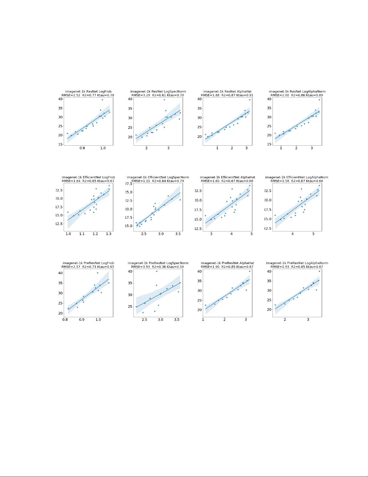
Predicting trends in the qualit y of state-of-the-art neural net w orks without access to training or testing data ∗ Charles H. Martin † T ongsu (Serena) P eng ‡ Mic hael W. Mahoney §¶ Abstract In many applications, one works with neural netw ork mo dels trained b y someone else. F or suc h pretrained mo dels, one may not ha ve access to training data or test data. Moreo ver, one may not kno w details ab out the mo del, e.g., the speciﬁcs of the training data, the loss function, the h yp erparameter v alues, etc. Giv en one or many pretrained models, it is a c hallenge to say an ything ab out the exp ected p erformance or quality of the models. Here, we address this c hallenge by pro viding a detailed meta-analysis of hundreds of publicly-av ailable pretrained mo dels. W e examine norm based capacity con trol metrics as w ell as p o wer la w based metrics from the recen tly-developed Theory of Hea vy-T ailed Self Regularization. W e ﬁnd that norm based metrics correlate well with rep orted test accuracies for w ell-trained models, but that they often cannot distinguish w ell-trained versus p oorly-trained mo dels. W e also ﬁnd that p o w er law based metrics can do muc h b etter—quan titatively b etter at discriminating among series of w ell-trained mo dels with a given architecture; and qualitatively b etter at discriminating well-trained v ersus p o orly-trained mo dels. These metho ds can b e used to iden tify when a pretrained neural netw ork has problems that cannot b e detected simply b y examining training/test accuracies. 1 In tro duction A common problem in machine learning (ML) is to ev aluate the quality of a given mo del. A p opular w a y to accomplish this is to train a mo del and then ev aluate its training/testing error. There are man y problems with this approac h. The training/testing curv es giv e very limited insigh t into the o verall prop erties of the mo del; they do not take in to account the (often large h uman and CPU/GPU) time for hyperparameter ﬁddling; they t ypically do not correlate with other prop erties of interest suc h as robustness or fairness or interpretabilit y; and so on. A related problem, in particular in industrial-scale artiﬁcial intelligence (AI), arises when the mo del user is not the mo del developer. Then, one ma y not ha ve access to the training data or the testing data. Instead, one may simply b e given a mo del that has already b een trained—a pretrained mo del—and need to use it as-is, or to ﬁne-tune and/or compress it and then use it. Na ¨ ıv ely—but in our exp erience commonly , among ML practitioners and ML theorists—if one do es not ha v e access to training or testing data, then one can sa y absolutely nothing ab out the qualit y of a ML mo del. This ma y b e true in w orst-case theory , but models are used in practice, and there is a need for a practical theory to guide that practice. Moreo ver, if ML is to b ecome ∗ T o app ear in Natur e Communic ations . † Calculation Consulting, 8 Lo c ksley Av e, 6B, San F rancisco, CA 94122, charles@CalculationConsulting.com . ‡ Calculation Consulting, 8 Lo c ksley Av e, 6B, San F rancisco, CA 94122, serenapeng7@gmail.com . § ICSI and Departmen t of Statistics, Univ ersity of California at Berk eley , Berk eley , CA 94720, mmahoney@stat.berkeley.edu . ¶ Corresp onding author. 1 an industrial pro cess, then that pro cess will become compartmen talized in order to scale: some groups will gather data, other groups will dev elop models, and other groups will use those models. Users of mo dels cannot b e exp ected to know the precise details of ho w mo dels w ere built, the sp eciﬁcs of data that were used to train the mo del, what was the loss function or hyperparameter v alues, ho w precisely the mo del w as regularized, etc. Moreo ver, for man y large scale, practical applications, there is no ob vious w ay to deﬁne an ideal test metric. F or example, mo dels that generate fake text or con versational c hatb ots ma y use a proxy , lik e p erplexit y , as a test metric. In the end, ho wev er, they really require h uman ev aluation. Alternativ ely , mo dels that cluster user proﬁles, which are widely used in areas such as mark eting and adv ertising, are unsup ervised and ha ve no ob vious lab els for comparison and/or ev aluation. In these and other areas, ML ob jectives can be po or pro xies for downstream goals. Most importantly , in industry , one faces unique practical problems such as determining whether one has enough data for a given model. Indeed, high quality , lab eled data can b e v ery exp ensiv e to acquire, and this cost can mak e or break a pro ject. Metho ds that are developed and ev aluated on any well-deﬁned publicly-a v ailable corpus of data, no matter how large or diverse or in teresting, are clearly not going to b e well-suited to address problems such as this. It is of great practical in terest to hav e metrics to ev aluate the quality of a trained mo del—in the absence of training/testing data and without any detailed knowledge of the training/testing pro cess. There is a need for a practical theory for pretrained mo dels which can predict how, when, and why suc h mo dels can b e exp ected to p erform well or p o orly . In the absence of training and testing data, ob vious quantities to examine are the w eight matrices of pretrained mo dels, e.g., properties such as norms of weigh t matrices and/or parameters of Po wer La w (PL) ﬁts of the eigenv alues of weigh t matrices. Norm-based metrics hav e b een used in traditional statistical learning theory to b ound capacity and construct regularizers; and PL ﬁts are based on statistical mechanics approac hes to deep neural netw orks (DNNs). While we use traditional norm-based and PL-based metrics, our goals are not the traditional goals. Unlike more common ML approaches, we do not seek a b ound on the generalization (e.g., by ev aluating training/test errors), w e do not seek a new regularizer, and w e do not aim to ev aluate a single mo del (e.g., as with h yp erparameter optimization). Instead, we w ant to examine diﬀeren t mo dels across common architecture series, and we wan t to compare models b etw een diﬀerent architectures themselv es. In b oth cases, one can ask whether it is possible to predict trends in the quality of pretrained DNN mo dels without access to training or testing data. T o answer this question, w e pro vide a detailed empirical analysis, ev aluating quality metrics for pretrained DNN mo dels, and we do so at scale. Our approac h ma y be view ed as a statistical meta- analysis of previously published work, where we consider a large suite of hundreds of publicly- a v ailable mo dels, mostly from computer vision (CV) and natural language pro cessing (NLP). By now, there are man y suc h state-of-the-art mo dels that are publicly-a v ailable, e.g., h undreds of pretrained mo dels in CV ( ≥ 500) and NLP ( ≈ 100). 1 F or all these mo dels, we hav e no access to training data or testing data, and we hav e no sp eciﬁc knowledge of the training/testing proto cols. Here is a summary of our main results. First, norm-based metrics do a reasonably go od job at predicting qualit y trends in well-trained CV/NLP mo dels. Second, norm-based metrics ma y give spurious results when applied to p oorly-trained mo dels (e.g., mo dels trained without enough data, etc.). F or example, they ma y exhibit what w e call Scale Collapse for these mo dels. Third, PL-based metrics can do muc h b etter at predicting quality trends in pretrained CV/NLP mo dels. In particular, a weigh ted PL exp onen t (weigh ted by the log of the sp ectral norm of the corresp onding lay er) is quantitativ ely b etter at discriminating among a series of well- 1 When we b egan this work in 2018, there were few er than tens of such models; now in 2020, there are hundreds of such mo dels; and we exp ect that in a year or tw o there will b e an order of magnitude or more of such mo dels. 2 trained versus very-w ell-trained mo dels within a giv en architecture series; and the (un weigh ted) a verage PL exp onen t is qualitativ ely b etter at discriminating well-trained versus p o orly-trained mo dels. F ourth, PL-based metrics can also b e used to characterize ﬁne-scale mo del prop erties, including what we call lay er-wise Correlation Flow, in w ell-trained and p oorly-trained mo dels; and they can b e used to ev aluate mo del enhancements (e.g., distillation, ﬁne-tuning, etc.). Our w ork provides a theoretically-principled empirical ev aluation—b y far the largest, most detailed, and most comprehensive to date—and the theory w e apply w as dev elop ed previously [ 1 , 2 , 3 ]. P erforming suc h a meta-analysis of previously-published work is common in certain areas, but it is quite rare in ML, where the emphasis is on developing b etter training proto cols. 2 Results After describing our ov erall approach, we study in detail three well-kno wn CV architecture series (the VGG, ResNet, and DenseNet series of mo dels). Then, we lo ok in detail at several v ariations of a p opular NLP arc hitecture series (the Op enAI GPT and GPT2 series of mo dels), and w e presen t results from a broader analysis of hundreds of pretrained DNN mo dels. 2.1 Ov erall approac h Consider the ob jectiv e/optimization function (parameterized b y W l s and b l s) for a DNN with L la yers, and weigh t matrices W l and bias vectors b l , as the minimization of a general loss function L ov er the training data instances and lab els, { x i , y i } ∈ D . F or a t ypical sup ervised classiﬁcation problem, the goal of training is to construct (or learn) W l and b l that capture correlations in the data, in the sense of solving argmin W l , b L N X i =1 L ( E DN N ( x i ) , y i ) , (1) where the loss function L ( · , · ) can take on a m yriad of forms [ 4 ], and where the energy (or optimization) landscap e function E DN N = f ( x i ; W 1 , . . . , W L , b 1 , . . . , b L ) (2) dep ends parametrically on the weigh ts and biases. F or a trained mo del, the form of the function E DN N do es not explicitly dep end on the data (but it do es explicitly dep end on the weigh ts and biases). The function E DN N maps data instance v ectors ( x i v alues) to predictions ( y i lab els), and th us the output of this function do es dep end on the data. Therefore, one can analyze the form of E DN N in the absence of any training or test data. T est accuracies ha ve b een rep orted online for publicly-a v ailable pretrained pyT orc h models [ 5 ]. These mo dels hav e b een trained and ev aluated on lab eled data { x i , y i } ∈ D , using standard tec hniques. W e do not ha v e access to this data, and we hav e not trained an y of the mo dels ourselv es. Our metho dological approach is th us similar to a statistical meta-analysis, common in biomedical research, but uncommon in ML. Computations were p erformed with the publicly- a v ailable WeightWatcher to ol (v ersion 0.2.7) [ 6 ]. T o b e fully reproducible, w e only examine publicly-a v ailable, pretrained mo dels, and we provide all Jupyter and Go ogle Colab noteb ooks used in an accompanying github rep ository [ 7 ]. See the Supplementary Information for details. Metrics for DNN W eight Matrices. Our approac h in volv es analyzing individual DNN w eight matrices, for (dep ending on the architecture) fully-connected and/or conv olutional la yers. Eac h DNN lay er contains one or more lay er 2D N l × M l w eight matrices, W l , or pre-activ ation 3 maps, W i,l , e.g., extracted from 2D Conv olutional lay ers, where N > M . See the Supplemen tary Information for details. (W e may drop the i and/or i, l subscripts b elo w.) The b est p erform- ing quality metrics dep end on the norms and/or sp ectral prop erties of each weigh t matrix, W , and/or, equiv alen tly , it’s empirical correlation matrix, X = W T W . T o ev aluate the quality of state-of-the-art DNNs, we consider the following metrics: F rob enius Norm: k W k 2 F = k X k F = X M i =1 λ i (3) Sp ectral Norm: k W k 2 ∞ = k X k ∞ = λ max (4) W eighted Alpha: ˆ α = α log λ max (5) α -Norm (or α -Shatten Norm): k W k 2 α 2 α = k X k α α = X M i =1 λ α i . (6) T o p erform diagnostics on p oten tially-problematic DNNs, we will decomp ose ˆ α into its t wo com- p onen ts, α and λ max . Here, λ i is the i th eigen v alue of the X , λ max is the maximum eigen v alue, and α is the ﬁtted PL exponent. These eigenv alues are squares of the singular v alues σ i of W , λ i = σ 2 i . All four metrics can b e computed easily from DNN weigh t matrices. The ﬁrst tw o metrics are well-kno wn in ML. The last tw o metrics deserve sp ecial mention, as they dep end on an empirical parameter α that is the PL exp onen t that arises in the recently-dev elop ed Heavy T ailed Self Regularization (HT-SR) Theory [ 1 , 2 , 3 ]. Ov erview of Hea vy-T ailed Self-Regularization. In the HT-SR Theory , one analyzes the eigen v alue sp ectrum, i.e., the Empirical Sp ectral Density (ESD), of the asso ciated correlation matrices [ 1 , 2 , 3 ]. F rom this, one characterizes the amoun t and form of correlation, and therefore implicit self-regularizartion, present in the DNN’s w eight matrices. F or eac h lay er weigh t matrix W , of size N × M , construct the asso ciated M × M (uncentered) correlation matrix X . Dropping the L and l , i indices, one has X = 1 N W T W . If we compute the eigen v alue sp ectrum of X , i.e., λ i suc h that Xv i = λ i v i , then the ESD of eigen v alues, ρ ( λ ), is just a histogram of the eigenv alues, formally written as ρ ( λ ) = P M i =1 δ ( λ − λ i ) . Using HT-SR Theory , one c haracterizes the correlations in a w eight matrix by examining its ESD, ρ ( λ ). It can b e w ell-ﬁt to a truncated PL distribution, given as ρ ( λ ) ∼ λ − α , (7) whic h is (at least) v alid within a b ounded range of eigenv alues λ ∈ [ λ min , λ max ]. The original work on HT-SR Theory considered a small n umber of NNs, including AlexNet and InceptionV3. It show ed that for nearly every W , the (bulk and tail) of the ESDs can b e ﬁt to a truncated PL, and that PL exp onen ts α nearly all lie within the range α ∈ (1 . 5 , 5) [ 1 , 2 , 3 ]. As for the mechanism resp onsible for these prop erties, statistical physics oﬀers sev eral p ossibilities [ 8 , 9 ], e.g., self organized criticality [ 10 , 11 ] or m ultiplicativ e noise in the sto c hastic optimization algorithms used to train these mo dels [ 12 , 13 ]. Alternativ ely , related tec hniques ha ve b een used to analyze correlations and information prop ogation in actual spiking neurons [ 14 , 15 ]. Our meta-analysis do es not require knowledge of mec hanisms; and it is not even clear that one mec hanism is resp onsible for ev ery case. Crucially , HT-SR Theory predicts that smaller v alues of α should corresp ond to mo dels with b etter correlation ov er multiple size scales and thus to b etter mo dels. The notion of “size scale” is well-deﬁned in ph ysical systems, to which this style of analysis is usually applied, but it is less well-deﬁned in CV and NLP applications. Informally , it would corresp ond to pixel groups that are at a greater distance in some metric, or b et ween 4 sen tence parts that are at a greater distance in text. Relatedly , previous work observed that smaller exp onen ts α corresp ond to more implicit self-regularization and b etter generalization, and that we exp ect a linear correlation b et ween ˆ α and mo del quality [ 1 , 2 , 3 ]. DNN Empirical Quality Metrics. F or norm-based metrics, w e use the av erage of the log norm, to the appropriate pow er. Informally , this amounts to assuming that the la yer w eight matrices are statistically indep endent, in which case w e can estimate the mo del complexity C , or test accuracy , with a standard Pro duct Norm (which resembles a data dep enden t V C complexit y), C ∼ k W 1 k × k W 2 k × · · · × k W L k , (8) where k · k is a matrix norm. The log complexity , log C ∼ log k W 1 k + log k W 2 k + · · · + log k W L k = X l log k W l k , (9) tak es the form of an a verage Log Norm. F or the F rob enius Norm metric and Sp ectral Norm metric, we can use Eqn. ( 9 ) directly (since, when taking log k W l k 2 F , the 2 comes do wn and out of the sum, and thus ignoring it only changes the metric by a constant factor). The W eighted Alpha metric is an av erage of α l o ver all la yers l ∈ { 1 , . . . , l } , w eighted by the size, or scale, or each matrix, ˆ α = 1 L X l α l log λ max,l ≈ h log k X k α α i , (10) where L is the total num b er of la yer w eight matrices. The W eighted Alpha metric w as in tro duced previously [ 3 ], where it was sho wn to correlate well with trends in rep orted test accuracies of pretrained DNNs, alb eit on a m uch smaller and more limited set of models than we consider here. Based on this, in this pap er, w e introduce and ev aluate the α -Shatten Norm metric, X l log k X l k α l α l = X l α l log k X l k α l . (11) F or the α -Shatten Norm metric, α l v aries from lay er to lay er, and so in Eqn. ( 11 ) it cannot b e tak en out of the sum. F or small α , the W eighted Alpha metric approximates the Log α -Shatten norm, as can be shown with a statistical mec hanics and random matrix theory deriv ation; and the W eighted Alpha and α -Shatten norm metrics often b eha ve lik e an impro ved, weigh ted av erage Log Sp ectral Norm. Finally , although it do es less well for predicting trends in state-of-the-art mo del series, e.g., as depth changes, the av erage v alue of α , i.e., ¯ α = 1 L X l α l = h α i , (12) can b e used to p erform mo del diagnostics, to identify problems that cannot b e detected by examin- ing training/test accuracies, and to discriminate p oorly-trained mo dels from well-trained mo dels. One determines α for a given la yer b y ﬁtting the ESD of that la yer’s w eight matrix to a truncated PL, using the commonly accepted Maximum Likelihoo d metho d [ 16 , 17 ]. This metho d w orks v ery well for exp onen ts b et w een α ∈ (2 , 4); and it is adequate, although imprecise, for smaller and esp ecially larger α [ 18 ]. Op erationally , α is determined by using the WeightWatcher to ol [ 6 ] to ﬁt the histogram of eigen v alues, ρ ( λ ), to a truncated PL, ρ ( λ ) ∼ λ α , λ ∈ [ λ min , λ max ] , (13) 5 Figure 1: Sc hematic of analyzing DNN lay er w eight matrices W . Giv en an individual la yer w eight matrix W , from either a fully-connected lay er or a conv olutional lay er, p erform a Singular V alue Decomp osition (SVD) to obtain W = UΣV T , and examine the histogram of eigen v alues of W T W . Norm-based metrics and PL-based metrics (that dep end on ﬁtting the histogram of eigen v alues to a truncated PL) can be used to compare models. F or example, one can analyze one la yer of a pre-trained mo del, compare multiple lay ers of a pre-trained mo del, make comparisons across mo del arc hitectures, monitor neural netw ork prop erties during training, etc. where λ max is the largest eigenv alue of X = W T W , and where λ min is selected automatically to yield the b est (in the sense of minimizing the K-S distance) PL ﬁt. Each of these quantities is deﬁned for a given lay er W matrix. See Figure 1 for an illustration. T o a void confusion, let us clarify the relationship b et ween α and ˆ α . W e ﬁt the ESD of the correlation matrix X to a truncated PL, parameterized by 2 v alues: the PL exp onen t α , and the maxim um eigen v alue λ max . The PL exp onen t α measures the amount of correlation in a DNN la yer weigh t matrix W . It is v alid for λ ≤ λ max , and it is scale-in v arian t, i.e., it do es not dep end on the normalization of W or X . The λ max is a measure of the size, or scale, of W . Multiplying eac h α b y the corresp onding log λ max w eighs “bigger” lay ers more, and av eraging this pro duct leads to a balanced, W eigh ted Alpha metric ˆ α for the en tire DNN. W e will see that for w ell-trained CV and NLP mo dels, ˆ α p erforms quite well and as exp ected, but for CV and NLP mo dels that are p oten tially-problematic or less w ell-trained, metrics that dep end on the scale of the problem can p erform anomalously . In these cases, separating ˆ α in to its t wo comp onen ts, α and λ max , and examining the distributions of each, can b e helpful. 2.2 Comparison of CV mo dels Eac h of the V GG, ResNet, and DenseNet series of mo dels consists of several pretrained DNN mo dels, with a given base architecture, trained on the full ImageNet [ 19 ] dataset, and each is distributed with the curren t op en source p yT orch framew ork (version 1.4) [ 20 ]. In addition, w e examine a larger set of ResNet mo dels, which w e call the ResNet-1K series, trained on the ImageNet-1K dataset [ 19 ] and provided on the OSMR Sandb o x [ 5 ]. F or these mo dels, we ﬁrst p erform coarse mo del analysis, comparing and contrasting the four mo del series, and predicting trends in mo del quality . W e then p erform ﬁne lay er analysis, as a function of depth. This lay er analysis go es b ey ond predicting trends in model quality , instead illustrating that PL-based metrics can provide nov el insigh ts among the VGG, ResNet/ResNet-1K, and DenseNet architectures. 6 Series # Metric h log k W k 2 F i h log k W k 2 ∞ i ˆ α h log k X k α α i V GG 6 RMSE 0.56 0.23 0.48 0.34 R 2 0.88 0.98 0.92 0.96 Kendall- τ -0.79 -0.93 -0.93 -0.93 ResNet 5 RMSE 0.9 0.97 0.61 0.66 R 2 0.92 0.9 0.96 0.9 Kendall- τ -1.0 -1.0 -1.0 -1.0 ResNet- 1K 19 RMSE 2.4 2.8 1.8 1.9 R 2 0.81 0.74 0.89 0.88 Kendall- τ -0.79 -0.79 -0.89 -0.88 DenseNet 4 RMSE 0.3 0.11 0.16 0.21 R 2 0.93 0.99 0.98 0.97 Kendall- τ -1.0 -1.0 -1.0 -1.0 T able 1: Qualit y metrics (for RMSE, smaller is b etter; for R 2 , larger is b etter; and for Kendall- τ rank correlation, larger magnitude is b etter) for rep orted T op1 test error for pretrained models in each architecture series. Column # refers to num b er of mo dels. VGG, ResNet, and DenseNet w ere pretrained on ImageNet. ResNet-1K was pretrained on ImageNet-1K. Av erage Qualit y Metrics versus Rep orted T est Accuracies. W e examine the p erfor- mance of the four quality metrics—Log F rob enius norm ( h log k W k 2 F i ), Log Sp ectral norm ( h log k W k 2 ∞ i ), W eighted Alpha ( ˆ α ), and Log α -Norm ( h log k X k α α i )—applied to each of the V GG, ResNet, ResNet-1K, and DenseNet series. Figure 2 plots the four quality metrics versus rep orted test accuracies [ 20 ], 2 as w ell as a basic linear regression line, for the VGG series. Here, smaller norms and smaller v alues of ˆ α imply b etter generalization (i.e., greater accuracy , low er error). Quan- titativ ely , Log Sp ectral norm is the b est; but, visually , all four metrics correlate quite well with rep orted T op1 accuracies. The DenseNet series has similar b eha vior. (These and many other suc h plots can b e seen on our publicly-av ailable rep o.) T o examine visually how the four quality metrics dep end on data set size on a larger, more complex mo del series, w e next lo ok at results on ResNet versus ResNet-1K. Figure 3 compares the Log α -Norm metric for the full ResNet mo del, trained on the full ImageNet dataset, against the ResNet-1K mo del, trained on a muc h smaller ImageNet-1K data set. Here, the Log α -Norm is muc h b etter than the Log F rob enius/Sp ectral norm metrics (although, as T able 1 shows, it is sligh tly w orse than the W eigh ted Alpha metric). The ResNet series has strong correlation (RMSE of 0 . 66, R 2 of 0 . 9, and Kendall- τ of − 1 . 0), whereas the ResNet-1K series also shows go od but w eaker correlation (muc h larger RMSE of 1 . 9, R 2 of 0 . 88, and Kendall- τ of − 0 . 88). See T able 1 for a summary of results for T op1 accuracies for all four metrics for the V GG, ResNet, ResNet-1K, and DenseNet series. Similar results are obtained for the T op5 accuracies. The Log F rob enius norm p erforms well but not extremely well; the Log Sp ectral norm p erforms v ery w ell on smaller, simpler models lik e the V GG and DenseNet architectures; and, when mo ving to the larger, more complex ResNet series, the PL-based metrics, W eigh ted Alpha and the Log α -Norm, p erform the b est. Overall, though, these mo del series are all v ery well-trodden; and our results indicate that norm-based metrics and PL-based metrics can b oth distinguish among a se- ries of well-trained v ersus very-w ell-trained mo dels, with PL-based metrics p erforming somewhat (i.e., quantitativ ely) b etter on the larger, more complex ResNet series. In particular, the PL-based W eigh ted Alpha and Log α -Norm metrics tend to perform b et- ter when there is a wider v ariation in the hyperparameters, going beyond just increasing the 2 These test accuracies hav e been previously rep orted and made publicly-a v ailable by others. W e take them as giv en. W e do not attempt to repro duce/v erify them, since we do not p ermit ourselves access to training/test data. 7 (a) Log F rob enius Norm, VGG (b) Log Sp ectral Norm, VGG (c) W eighted Alpha, VGG (d) Log α -Norm, VGG Figure 2: Comparison of Average Log Norm and W eighted Alpha quality metrics versus rep orted test accuracy for pretrained VGG mo dels: VGG11, VGG13, VGG16, and VGG19, with and without Batc h Normalization (BN), trained on ImageNet, av ailable in pyT orc h (v1.4). Metrics ﬁt by linear regression, RMSE, R2, and the Kendal-tau rank correlation metric rep orted. depth. In addition, sometimes the purely norm-based metrics such as the Log Sp ectral norm can b e uncorrelated or even anti-correlated with the test accuracy , while the PL-metrrics are p ositiv ely-correlated. This is seen in the Supplementary Information, ShuﬄeNet in Figure 10(b) , SqueezeNext in Figure 11(j) , and WRN in Figure 15(f ) ). Going b ey ond coarse av erages to examining quality metrics for each lay er weigh t matrix as a function of depth (or lay er id), our metrics can b e used to p erform mo del diagnostics and to iden tify ﬁne-scale prop erties in a pretrained model. Doing so inv olves separating ˆ α in to its t wo comp onen ts, α and λ max , and examining the distributions of eac h. W e provide examples of this. La y er Analysis: Metrics as a F unction of Depth. Figure 4 plots the PL exp onen t α , as a function of depth, for eac h lay er (ﬁrst lay er corresp onds to data, last la yer to lab els) for the least accurate (shallow est) and most accurate (deep est) mo del in each of the VGG (no BN), ResNet, and DenseNet series. (Man y more suc h plots are av ailable at our rep o.) In the V GG mo dels, Figure 4(a) sho ws that the PL exp onen t α systematically increases as w e mov e do wn the netw ork, from data to lab els, in the Conv2D lay ers, starting with α . 2 . 0 and reac hing all the wa y to α ∼ 5 . 0; and then, in the last three, large, fully-connected (FC) la yers, α stabilizes back down to α ∈ [2 , 2 . 5]. This is seen for all the V GG mo dels (again, only the shallow est and deep est are shown), indicating that the main eﬀect of increasing depth is to 8 (a) ResNet, Log α -Norm (b) ResNet-1K, Log α -Norm Figure 3: Comparison of Average α -Norm quality metric versus rep orted T op1 test accuracy for the ResNet and ResNet-1K pretrained (pyT orc h) mo dels. Metrics ﬁt by linear regression, RMSE, R2, and the Kendal-tau rank correlation metric rep orted. increase the range ov er which α increases, thus leading to larger α v alues in later Conv2D lay ers of the VGG mo dels. This is quite diﬀerent than the b eha vior of either the ResNet-1K mo dels or the DenseNet mo dels. F or the ResNet-1K mo dels, Figure 4(b) sho ws that α also increases in the last few la y ers (more dramatically than for V GG, observ e the diﬀering scales on the Y axes). Ho wev er, as the ResNet-1K mo dels get deep er, there is a wide range ov er which α v alues tend to remain small. This is seen for other mo dels in the ResNet-1K series, but it is most pronounced for the larger ResNet-1K (152) mo del, where α remains relatively stable at α ∼ 2 . 0, from the earliest la yers all the wa y until w e reach close to the ﬁnal lay ers. F or the DenseNet mo dels, Figure 4(c) shows that α tends to increase as the lay er id increases, in particular for la yers tow ard the end. While this is similar to the VGG mo dels, with the DenseNet models, α v alues increase almost immediately after the ﬁrst few lay ers, and the v ariance is muc h larger (in particular for the earlier and middle lay ers, where it can range all the wa y to α ∼ 8 . 0) and muc h less systematic throughout the netw ork. Ov erall, Figure 4 demonstrates that the distribution of α v alues among lay ers is architecture dep enden t, and that it can v ary in a systematic w ay within an arc hitecture series. This is to b e exp ected, since some arc hitectures enable b etter extraction of signal from the data. This also suggests that, while p erforming very well at predicting trends within an arc hitecture series, PL-based metrics (as well as norm-based metrics) should b e used with caution when comparing mo dels with v ery diﬀerent architectures. Correlation Flow; or Ho w α V aries Across La y ers. Figure 4 can b e understo o d in terms of what w e will call Correlation Flo w. Recall that the av erage Log α -Norm metric and the W eighted Alpha metric are based on HT-SR Theory [ 1 , 2 , 3 ], which is in turn based on the statistical mechanics of hea vy tailed and strongly correlated systems [ 21 , 8 , 22 , 23 ]. There, one exp ects that the weigh t matrices of well-trained DNNs will exhibit correlations ov er man y size scales, as is well-kno wn in other strongly-correlated systems [ 21 , 8 ]. This w ould imply that their ESDs can b e well-ﬁt b y a truncated PL, with exp onen ts α ∈ [2 , 4]. Muc h larger v alues ( α  6) ma y reﬂect p o orer PL ﬁts, whereas smaller v alues ( α ∼ 2), are associated with mo dels that generalize b etter. Informally , one w ould exp ect a DNN model to perform well when it facilitates the propagation 9 (a) VGG (b) ResNet (c) DenseNet (d) ResNet (ov erlaid) Figure 4: PL exp onen t ( α ) v ersus lay er id, for the least and the most accurate mo dels in VGG (a), ResNet (b), and DenseNet (c) series. (VGG is without BN; and note that the Y axes on eac h plot are diﬀeren t.) Subﬁgure (d) displays the ResNet mo dels (b), zo omed in to α ∈ [1 , 5], and with the lay er ids ov erlaid on the X-axis, from smallest to largest, to allow a more detailed analysis of the most strongly correlated lay ers. Notice that ResNet152 exhibits diﬀerent and m uch more stable b eha vior of α across lay ers. This contrasts with how b oth VGG mo dels gradually w orsen in deep er lay ers and ho w the DenseNet mo dels are muc h more erratic. In the text, this is in terpreted in terms of Correlation Flow. of information/features across lay ers. In the absence of training/test data, one might h yp othesize that this ﬂow of information leav es empirical signatures on w eight matrices, and that we can quan tify this b y measuring the PL prop erties of w eight matrices. In this case, smaller α v alues corresp ond to lay ers in which information correlations b et ween data across multiple scales are b etter captured [ 1 , 8 ]. This leads to the h yp othesis that small α v alues that are stable across m ul- tiple lay ers enable b etter correlation ﬂow through the net work. This is similar to recen t work on the information b ottlenec k [ 24 , 25 ], except that here w e w ork in an en tirely unsup ervised setting. Scale Collapse; or How Distillation Ma y Break Mo dels. The similarity b et ween norm- based metrics and PL-based metrics may lead one to w onder whether the W eighted Alpha metric is just a v ariation of more familiar norm-based metrics. Among h undreds of pretrained mo dels, there are “exceptions that prov e the rule,” and these can b e used to sho w that ﬁtted α v alues do contain information not captured b y norms. T o illustrate this, we sho w that some compres- sion/distillation metho ds [ 26 ] may actually damage mo dels unexp ectedly , by in tro ducing what 10 (a) λ max for ResNet20 lay ers (b) α for ResNet20 lay ers Figure 5: ResNet20, distilled with Group Regularization, as implemen ted in the distiller (4D regularized 5Lremov ed) pretrained mo dels. Log Sp ectral Norm (log λ max ) and PL exp onen t ( α ) for individual lay ers, v ersus la yer id, for b oth baseline (b efore distillation, green) and ﬁne- tuned (after distillation, red) pretrained mo dels. w e call Scale Collapse, where several distilled la yers ha ve unexpectedly small Sp ectral Norms. By Scale Collapse, we mean that the size scale, e.g., as measured by the Sp ectral or F rob enius Norm, of one or more lay ers changes dramatically , while the size scale of other lay ers changes very little, as a function of some change to or p erturbation of a mo del. The size scales of diﬀerent parts of a DNN mo del are typically deﬁned implicitly by the mo del training pro cess, and they t ypically v ary in a gradual wa y for high-qualit y mo dels. Examples of changes of interest include mo del compression or distillation (discussed here for a CV mo del), data augmentation (discussed b elo w for an NLP mo del), additional training, mo del ﬁne-tuning, etc. Consider ResNet20, trained on CIF AR10, b efore and after applying the Group Regularization distillation technique, as implemented in the distiller pac k age [ 27 ]. W e analyze the pretrained 4D regularized 5Lremov ed baseline and ﬁne-tuned mo dels. The rep orted baseline test accuracies (T op1= 91 . 45 and T op5= 99 . 75) are b etter than the rep orted ﬁne-tuned test accuracies (T op1= 91 . 02 and T op5= 99 . 67). Because the baseline accuracy is greater, the previous results on ResNet (T able 1 and Figure 3 ) suggest that the baseline Sp ectral Norms should b e smaller on av erage than the ﬁne-tuned ones. The opp osite is observ ed. Figure 5 presen ts the Sp ectral Norm (here denoted log λ max ) and PL exp onent ( α ) for eac h individual lay er w eigh t matrix W . On the other hand, the α v alues (in Figure 5(b) ) do not diﬀer systematically b et ween the baseline and ﬁne-tuned mo dels. Also, ¯ α , the av erage unw eighted baseline α , from Eqn. ( 12 ), is smaller for the original mo del than for the ﬁne-tuned mo del (as predicted by HT-SR Theory , the basis of ˆ α ). In spite of this, Figure 5(b) also depicts tw o v ery large α  6 v alues for the baseline, but not for the ﬁne-tuned, mo del. This suggests the baseline mo del has at least t wo o ver-parameterized/under- trained la yers, and that the distillation metho d do es, in fact, improv e the ﬁne-tuned mo del b y compressing these lay ers. Pretrained mo dels in the distiller pac k age ha ve passed some quality metric, but they are m uch less well tro dden than an y of the V GG, ResNet, or DenseNet series. The obvious in terpre- tation is that, while norms make go o d regularizers for a single mo del, there is no reason a priori to exp ect them correlate w ell with test accuracies across diﬀeren t mo dels, and they may not dif- feren tiate well-trained versus p oorly-trained mo dels. W e do exp ect, how ever, the PL α to do so, b ecause it eﬀectively measures the amoun t of information correlation in the mo del [ 1 , 2 , 3 ]. This suggests that the α v alues will improv e, i.e., decrease, ov er time, as distillation techniques con- 11 tin ue to impro ve. The reason for the anomalous behavior shown in Figure 5 is that the distiller Group Regularization technique causes the norms of the W pre-activ ation maps for tw o Conv2D la yers to increase spuriously . This is diﬃcult to diagnose by analyzing training/test curves, but it is easy to diagnose with our approach. 2.3 Comparison of NLP Mo dels Within the past few y ears, nearly 100 op en source, pretrained NLP DNNs based on the revolution- ary T ransformer arc hitecture hav e emerged. These include v ariants of BER T, T ransformer-XML, GPT, etc. The T ransformer architectures consist of blo c ks of so-called Atten tion lay ers, contain- ing tw o large, F eed F orward (Linear) weigh t matrices [ 28 ]. In contrast to smaller pre-Activ ation maps arising in Cond2D lay ers, Atten tion matrices are signiﬁcantly larger. In general, they hav e larger PL exp onen ts α . Based on HT-SR Theory (in particular, the interpretation of v alues of α ∼ 2 as modeling systems with goo d correlations o ver man y size scales [ 21 , 8 ]), this suggests that these models fail to capture successfully man y of the information correlations in the data (relativ e to their size) and thus are substantially under-trained. More generally , compared to CV mo dels, mo dern NLP mo dels hav e larger weigh t matrices and displa y diﬀerent sp ectral prop erties. While norm-based metrics perform reasonably well on well-trained NLP mo dels, they often b eha ve anomalously on p o orly-trained mo dels. F or such mo dels, weigh t matrices may displa y rank collapse, decreased F rob enius mass, or unusually small Spectral norms. This may b e mis- in terpreted as “smaller is b etter.” Instead, it should probably b e interpreted as b eing due to a similar mechanism to how distillation can “damage” otherwise go o d mo dels. In contrast to norm-based metrics, PL-based metrics, including the Log α -Norm metric and the W eigh ted Al- pha metric, displa y more consistent b eha vior, even on less well-trained mo dels. T o help identify when architectures need repair and when more and/or b etter data are needed, one can use these metrics, as w ell as the decomp osition of the W eigh ted Alpha metric ( α log λ max ) in to its PL comp onen t ( α ) and its norm comp onen t (log λ max ), for each lay er. Man y NLP mo dels, suc h as early v ariants of GPT and BER T, ha ve weigh t matrices with un usually large PL exp onen ts (e.g., α  6). This indicates these matrices may b e under-correlated (i.e., ov er-parameterized, relativ e to the amoun t of data). In this regime, the truncated PL ﬁt itself may not b e very reliable b ecause the Maximum Likelihoo d estimator it uses is unreliable in this range. In this case, the sp eciﬁc α v alues returned by the truncated PL ﬁts are less reliable, but having large versus small α is reliable. If the ESD is visually examined, one can usually describ e these W as in the Bulk-Deca y or Bulk-plus-Spikes phase from HT-ST Theory [ 1 , 2 ]. Previous work [ 1 , 2 ] has conjectured that v ery well-trained DNNs would not hav e many outlier α  6. Consisten t with this, more recen t improv ed versions of GPT (sho wn below) and BER T (not shown) conﬁrm this. Op enAI GPT Mo dels. The Op enAI GPT and GPT2 series of mo dels provide the opp ortunit y to analyze tw o eﬀects: increasing the sizes of b oth the data set and the architectures sim ultane- ously; and training the same mo del with low-qualit y data versus high-qualit y data. These mo dels ha ve the ability to generate fake text that app ears to the human to b e real, and they ha ve gener- ated media attention b ecause of the p oten tial for their misuse. F or this reason, the original GPT mo del released by Op enAI was trained on a deﬁcient data set, rendering the mo del interesting but not fully functional. Later, Op enAI released a muc h improv ed mo del, GPT2-small, which has the same arc hitecture and num b er of lay ers as GPT, but whic h has b een trained on a larger and b etter data set, making it remark ably go o d at generating (near) h uman-quality fake text. Sub- sequen t mo dels in the GPT2 w ere larger and trained to more data. By comparing GPT2-small to GPT2-medium to GPT2-large to GPT2-xl, we can examine the eﬀect of increasing data set 12 Series # h log k W k F i h log k W k ∞ i ˆ α h log k X k α α i GPT 49 1.64 1.72 7.01 7.28 GPT2-small 49 2.04 2.54 9.62 9.87 GPT2-medium 98 2.08 2.58 9.74 10.01 GPT2-large 146 1.85 1.99 7.67 7.94 GPT2-xl 194 1.86 1.92 7.17 7.51 T able 2: Av erage v alue for the a verage Log Norm and W eighted Alpha metrics for pretrained Op enAI GPT and GPT2 mo dels. Column # refers to num b er of lay ers treated. Averages do not include the ﬁrst embedding lay er(s) b ecause they are not (implicitly) normalized. GPT has 12 la yers, with 4 Multi-head A ttention Blo c ks, giving 48 lay er W eight Matrices, W . Eac h Blo c k has 2 comp onen ts, the Self A ttention (attn) and the Pro jection (pro j) matrices. Self-attention matrices are larger, of dimension (2304 × 768) or (3072 × 768). The pro jection la yer concatenates the self-atten tion results into a vector (of dimension 768). This gives 50 large matrices. Because GPT and GPT2 are trained on diﬀeren t data sets, the initial Embedding matrices diﬀer in shap e. GPT has an initial T oken and P ositional Embedding la y ers, of dimension (40478 × 768) and (512 × 768), resp ectiv ely , whereas GPT2 has input Embeddings of shap e (50257 × 768) and (1024 × 768), respectively . The Op enAI GPT2 (English) mo dels are: GPT2-small, GPT2-medium, GPT2-large, and GPT2-xl, having 12, 24, 36, and 48 lay ers, resp ectiv ely , with increasingly larger w eight matrices. and mo del size simultaneously , as well as analyze well-trained v ersus very-w ell-trained mo dels. By comparing the p o orly-trained GPT to the well-trained GPT2-small, we can identify empirical indicators for when a mo del has b een po orly-trained and th us ma y perform po orly when deplo yed. The GPT mo dels w e analyze are deploy ed with the p opular HuggingF ace PyT orch library [ 29 ]. Av erage Quality Metrics for GPT and GPT2. W e examine the p erformance of the four qualit y metrics (Log F rob enius norm, Log Sp ectral norm, W eighted Alpha, and Log α -Norm) for the Op enAI GPT and GPT2 pretrained mo dels. See T able 2 for a summary of results. Comparing trends b et ween GPT2-medium to GPT2-large to GPT2-xl, observe that (with one minor exception in volving the log F rob enius norm metric) all four metrics decrease as one go es from medium to large to xl. This indicates that the larger mo dels indeed lo ok b etter than the smaller mo dels, as exp ected. GPT2-small violates this general trend, but only very sligh tly . This could be due to under-optimization of the GPT2-small model, or since it is the smallest of the GPT2 series, and the metrics we present are most relev an t for mo dels at scale. Aside from this minor discrepancy , o v erall for these w ell-trained models, all these metrics no w b eha ve as expected, i.e., there is no Scale Collapse and norms are decreasing with increasing accuracy . Comparing trends b et w een GPT and GPT2-small rev eals a diﬀerent story . Observ e that all four metrics increase when going from GPT to GPT2-small, i.e., they are larger for the higher- qualit y mo del (higher quality since GPT2-small was trained to b etter data) and smaller for the lo wer-qualit y mo del, when the num b er of la yers is held ﬁxed. This is unexp ected. Here, to o, w e can p erform mo del diagnostics, by separating ˆ α into its tw o comp onen ts, α and λ max , and examining the distributions of each. In doing so, we see additional examples of Scale Collapse and additional evidence for Correlation Flow. La y er Analysis: Scale Collapse in GPT and GPT2. W e next examine the Sp ectral norm in GPT versus GPT2-small. In Figure 6(a) , the p o orly-trained GPT mo del has a smaller mean/median Spectral norm as w ell as, spuriously , many muc h smaller Spectral norms, compared 13 to the w ell-trained GPT2-small. This violates the con ven tional wisdom that smaller Sp ectral norms are b etter. Because there are so many anomalously small Sp ectral norms, the GPT mo del app ears to b e exhibiting a kind of Scale Collapse, like that observed (in Figure 5 ) for the distilled CV mo dels. This demonstrates that, while the Sp ectral (or F rob enius) norm may correlate well with predicted test error, at least among reasonably w ell-trained models, it is not a goo d indicator of the ov erall mo del qualit y in general. Na ¨ ıvely using it as an empirical quality metric may give spurious results when applied to p o orly-trained or otherwise deﬁcient mo dels. (a) Log Sp ectral Norm (log k W k ∞ ) (b) PL exp onen t ( α ) Figure 6: Histogram of PL exp onen ts and Log Sp ectral Norms for w eight matrices from the Op enAI GPT and GPT2-small pretrained mo dels. (a) Log Sp ectral Norm (log k W k ∞ ) (b) PL exp onen t ( α ) Figure 7: Log Spectral Norms (in (a)) and PL exp onen ts (in (b)) for w eight matrices from the Op enAI GPT and GPT2-small pretrained mo dels. (Note that the quan tities shown on eac h Y axis are diﬀeren t.) In the text, this is in terpreted in terms of Scale Collapse and Correlation Flow. Figure 7(a) shows the Sp ectral norm as a function of depth (lay er id). This illustrates tw o phenomenon. First, the large v alue of Sp ectral norm (in Figure 6(a) ) corresp onds to the ﬁrst em b edding la yer(s). These la yers ha ve a diﬀeren t eﬀectiv e normalization, and therefore a diﬀeren t scale. See the Supplementary Information for details. W e do not include them in our computed a verage metrics in T able 2 . Second, for GPT, there seems to b e t w o t yp es of lay ers with very diﬀeren t Sp ectral norms (an eﬀect which is seen, but to a m uch w eaker extent, for GPT2-small). Recall that attention mo dels hav e t w o t yp es of la yers, one small and large; and the Sp ectral norm (in particular, other norms do to o) displa ys unusually small v alues for some of these lay ers for GPT. This Scale Collapse for the po orly-trained GPT is similar to what w e observed for the distilled ResNet20 mo del in Figure 5(b) . Because of the anomalous Scale Collapse that is frequen tly observ ed in p oorly-trained models, these results suggest that scale-dep enden t norm metrics s h ould not b e directly applied to distinguish well-trained versus p oorly-trained mo dels. 14 La y er Analysis: Correlation Flow in GPT and GPT2. W e next examine the distribution of α v alues in GPT versus GPT2-small. Figure 6(b) sho ws the histogram (empirical densit y), for all lay ers, of α for GPT and GPT2-small. The older deﬁcient GPT has numerous un usually large α exp onen ts—meaning they are not well-described by a PL ﬁt. Indeed, we exp ect that a p o orly- trained mo del will lac k go o d (i.e., small α ) PL b eha vior in man y/most lay ers. On the other hand, the new er improv ed GPT2-small mo del has, on av erage, smaller α v alues than the older GPT, with all α ≤ 6 and with smaller mean/median α . It also has far fewer unusually-large outlying α v alues than GPT. F rom this (and other results not sho wn), we see that ¯ α from Eqn. ( 12 ), pro vides a go od quality metric for comparing the po orly-trained GPT v ersus the well-trained GPT2-small. This should b e contrasted with the b eha vior display ed by scale-dep enden t metrics such as the F rob enius norm (not shown) and the Sp ectral norm. This also reveals why ˆ α p erforms unusually in T able 2 . The PL exp onen t α b eha ves as expected, and thus the scale-inv arian t ¯ α metric lets us iden tify p oten tially p o orly-trained mo dels. It is the Scale Collapse that causes problems for ˆ α (recall that the scale enters into ˆ α via the weigh ts log λ max ). Figure 7(b) plots α versus the depth (lay er id) for each mo del. The deﬁcient GPT mo del displa ys tw o trends in α , one stable with α ∼ 4, and one increasing with la yer id, with α reac hing as high as 12. In contrast, the w ell-trained GPT2-small mo del shows consistent and stable patterns, again with one stable α ∼ 3 . 5 (and b elo w the GPT trend), and the other only sligh tly trending up, with α ≤ 6. These results show that the b eha vior of α across la yers diﬀers signiﬁcan tly b et ween GPT and GPT2-small, with the better GPT2-small lo oking more lik e the b etter ResNet-1K from Figure 4(b) . These results also suggest that smaller more stable v alues of α across depth is b eneﬁcial, i.e., that the Correlation Flo w is also a useful concept for NLP mo dels. GPT2: medium, large, xl. W e no w look across series of increasingly impro ving GPT2 mo dels (w ell-trained v ersus very-w ell-trained mo dels), by examining b oth the PL exp onen t α as well as the Log Norm metrics. Figure 8 sho ws the histograms ov er the lay er weigh t matrices for ﬁtted PL exp onen t α and the Log Alpha Norm metric. In general, and as exp ected, as w e mov e from GPT2-medium to GPT2-xl, histograms for b oth α exp onen ts and the Log Norm metrics downshift from larger to smaller v alues. F rom Figure 8(a) , w e see that ¯ α , the av erage α v alue, decreases with increasing mo del size (3 . 82 for GPT2-medium, 3 . 97 for GPT2-large, and 3 . 81 for GPT2-xl), although the diﬀerences are less noticeable b et w een the diﬀering well-trained v ersus very-w ell-trained GTP2 mo dels than b et w een the p oorly-trained versus w ell-trained GPT and GPT2-small mo dels. Also, from Figure 8(b) , we see that, unlike GPT, the lay er Log Alpha Norms b ehav e more as exp ected for GPT2 lay ers, with the larger mo dels consistently ha ving smaller norms (9 . 96 for GPT2-medium, 7 . 982 for GPT2- large, and 7 . 49 for GPT2-xl). Similarly , the Log Spectral Norm also decreases on a v erage with the larger models (2 . 58 for GPT2-medium, 1 . 99 for GPT2-large, and 1 . 92 for GPT2-xl). As expected, the norm metrics can indeed distinguish among well-trained versus very-w ell-trained mo dels. While the means and p eaks of the α distributions are getting smaller, tow ards 2 . 0, as ex- p ected, Figure 8(a) also sho ws that the tails of the α distributions shift right, with larger GPT2 mo dels having more unusually large α v alues. This is unexp ected. It suggests that these larger GPT2 mo dels are still under-optimized/ov er-parameterized (relative to the data on whic h they w ere trained) and that they hav e capacity to supp ort datasets even larger than the recent XL 1 . 5 B release [ 30 ]. This do es not con tradict recent theoretical work on the b eneﬁts of ov er- parameterization [ 31 ], e.g., since in practice these extremely large mo dels are not fully optimized. Subsequen t reﬁnements to these mo dels, and other mo dels suc h as BER T, indicate that this is lik ely the case. 15 (a) PL exp onen t ( α ) (b) Log Alpha Norm Figure 8: Histogram of PL exponents and Log Alpha Norm for w eight matrices from mo dels of diﬀeren t sizes in the GPT2 architecture series. (Plots omit the ﬁrst 2 (em b edding) la yers, because they are normalized diﬀerently giving anomalously large v alues.) log k · k 2 F log k · k 2 ∞ ˆ α log k · k α α RMSE (mean) 4.84 5.57 4.58 4.55 RMSE (std) 9.14 9.16 9.16 9.17 R2 (mean) 3.9 3.85 3.89 3.89 R2 (std) 9.34 9.36 9.34 9.34 Kendal-tau (mean) 3.84 3.77 3.86 3.85 Kendal-tau (std) 9.37 9.4 9.36 9.36 T able 3: Comparison of linear regression ﬁts for diﬀerent a verage Log Norm and W eigh ted Alpha metrics across 5 CV datasets, 17 architectures, co v ering 108 (out of o v er 400) diﬀeren t pretrained DNNs. W e include regressions only for architectures with ﬁve or more data p oin ts, and which are p ositiv ely correlated with test error. These results can b e readily repro duced using the Go ogle Colab noteb o oks. (See the Supplementary Information for details.) 2.4 Comparing Hundreds of Mo dels W e ha ve p erformed a large-scale analysis of hundreds of publicly-av ailable mo dels. This broader analysis is on a m uch larger set of CV and NLP mo dels, with a more diverse set of architectures, that ha v e b een developed for a wider range of tasks; and it complemen ts the previous more detailed analysis on CV and NLP mo dels, where w e hav e analyzed only a single arc hitecture series at a time. See the Supplementary Information (and our publicly-av ailable rep o) for details. T o quantify the relationship b et ween qualit y metrics and the rep orted test error and/or accuracy metrics, we use ordinary least squares to regress the metrics on the T op1 (and T op5) rep orted errors (as dep enden t v ariables), and w e rep ort the RMSE, the R 2 (R2) regresssion metric, and the Kendal- τ rank correlation metric. These include T op5 errors for the ImageNet-1K mo del, p ercen t error for the CIF AR-10/100, SVHN, CUB-200-2011 mo dels, and Pixel accuracy (Pix.Acc.) and In tersection-Over-Union (IOU) for other mo dels. W e regress them individually on each of the norm-based and PL-based metrics. Results are summarized in T able 3 (and Figures 9 – 17 of the Supplemen tary Information). F or the mean, smaller RMSE, larger R 2 , and larger Kendal- τ are desirable; and, for the standard deviation, smaller v alues are desirable. T ak en as a whole, ov er the en tire corpus of data, PL-based 16 metrics are somewhat better for b oth the R 2 mean and standard deviation; and PL-based metrics are m uch b etter for RMSE mean and standard deviation. Model diagnostics (Supplementary Information) indicate many outliers and imp erfect ﬁts. Overall, though, these and other results suggest our conclusions hold muc h more generally . 3 Discussion Comparison of V GG, ResNet, and DenseNet Architectures. Going b ey ond the goal of predicting trends in the qualit y of state-of-the-art neural netw orks without access to train- ing or testing data, obse rv ations suc h as the la yer-wise observ ations w e describ ed in Figure 4 can b e understo o d in terms of architectural diﬀerences b et ween VGG, ResNet, and DenseNet. V GG resembles the traditional con volutional architectures, such as LeNet5, and consists of sev- eral [Con v2D-Maxp ool-ReLu] blo c ks, follo wed by 3 large F ully Connected (F C) lay ers. ResNet greatly impro ved on V GG by replacing the large FC lay ers, shrinking the Conv2D blo c ks, and in tro ducing residual connections. This optimized approac h allo ws for greater accuracy with far few er parameters, and ResNet mo dels of up to 1000 lay ers hav e b een trained [ 32 ]. The eﬃciency and eﬀectiveness of ResNet seems to be reﬂected in the smaller and more stable α ∼ 2 . 0, across nearly all lay ers, indicating that the inner lay ers are very w ell correlated and more strongly optimized. This contrasts with the DenseNet mo dels, which contains man y connections b et ween ev ery la yer. These results (large α , meaning that even a PL model is probably a p oor ﬁt) suggest that DenseNet has to o man y connections, diluting high qualit y in teractions across lay ers, and leaving many lay ers very p o orly optimized. Fine-scale measuremen ts such as these enable us to form hypotheses as to the inner workings of DNN mo dels, op ening the door to an improv ed understanding of why DNNs w ork, as w ell as ho w to design b etter DNN mo dels. Correlation Flo w and Scale Collapse are tw o such examples. Related w ork. Statistical mechanics has long had inﬂuence on DNN theory and practice [ 33 , 34 , 35 ]. Our b est-p erforming PL-based metrics are based on statistical mechanics via HT-SR Theory [ 34 , 1 , 2 , 36 , 3 ]. The wa y in whic h we (and HT-SR Theory) use statistical mechanics theory is quite diﬀerent than the wa y it is more commonly formulated [ 33 , 35 ]. Going b eyond idealized mo dels, we use statistical mechanics in a broader sense, drawing up on techniques from quan titative ﬁnance, random matrix theory , and the statistical mechanics of heavy tailed and strongly correlated systems [ 21 , 8 , 22 , 23 ]. There is also a large b o dy of w ork in ML on using norm-based metrics to bound generalization error [ 37 , 38 , 39 ]. This theoretical w ork aims to pro v e generalization b ounds, and this applied work then uses these norms to construct regularizers to impro ve training. Proving generalization bounds and developing new regularizers is v ery diﬀeren t than our fo cus of v alidating pretrained mo dels. Our work also has in triguing similarities and diﬀerences with work on understanding DNNs with the information b ottlenec k principle [ 24 , 25 ], which p osits that DNNs can b e quan tiﬁed b y the mutual information b et ween their lay ers and the input and output v ariables. Most imp or- tan tly , our approach do es not require access to any data, while information measures used in the information b ottlenec k approach do require this. Nev ertheless, several results from HT-SR Theory , on which our metrics are based, hav e parallels in the information b ottlenec k approac h. P erhaps most notably , the quick transition from a Random-like phase to Bulk+Spikes phase, follo wed b y slow transition to a Hea vy-T ailed phase, as noted previously [ 1 ], is reminiscent of the dynamics on the Information Plane [ 25 ]. Finally , our w ork, starting in 2018 with the WeightWatcher to ol [ 6 ], is the ﬁrst to p erform a detailed analysis of the weigh t matrices of DNNs [ 1 , 2 , 3 ]. Subsequent to the initial version of 17 this pap er, w e b ecame a war e of tw o other w orks that were p osted to the in 2020 within w eeks of the initial version of this pap er [ 40 , 41 ]. Both of these pap ers v alidate our basic result that one can gain substantial insight in to mo del quality by examining weigh t matrices without access to any training or testing data. Ho w ever, b oth consider smaller mo dels drawn from a muc h narro wer range of applications than we consider. Previous results in HT-SR Theory suggest that insigh ts from these smaller models ma y not extend to the state-of-the-art CV and NLP mo dels w e consider. Conclusions. W e ha ve developed and ev aluated metho ds to predict trends in the quality of state-of-the-art neural netw orks—without access to training or testing data. Our main metho d- ology in volv ed weigh t matrix meta-analysis, using the publicly-av ailable WeightWatcher to ol [ 6 ], and informed by the recen tly-developed HT-SR Theory [ 1 , 2 , 3 ]. Prior to our work, it was not ev en ob vious that norm-based metrics w ould p erform well to predict trends in quality across mo dels (as they are usually used within a given mo del or parameterized mo del class, e.g., to b ound generalization error or to construct regularizers). Our results are the ﬁrst to demonstrate that they can b e used for this imp ortan t practical problem. Our results also demonstrate that PL-based metrics p erform b etter than norm-based metrics. This should not b e surprising—at least to those familiar with the statistical mechanics of heavy tailed and strongly correlated sys- tems [ 21 , 8 , 22 , 23 ]—since our use of PL exp onen ts is designed to capture the idea that w ell-trained mo dels capture information correlations o ver many size scales in the data. Again, though, our results are the ﬁrst to demonstrate this. Our approach can also b e used to pro vide ﬁne-scale insigh t (rationalizing the ﬂow of correlations or the collapse of size scale) throughout a netw ork. Both Correlation Flow and Scale Collapse are imp ortan t for improv ed diagnostics on pretrained mo dels as w ell as for improv ed training metho dologies. Lo oking forw ard. More generally , our results suggest what a practical theory of DNNs should lo ok like. T o see this, let’s distinguish b et w een tw o types of theories: non-empirical or analogical theories, in whic h one creates, often from general principles, a v ery simple toy mo del that can b e analyzed rigorously , and one then claims that the mo del is relev an t to the system of interest; and semi-empirical theories, in whic h there exists a rigorous asymptotic theory , which comes with parameters, for the system of in terest, and one then adjusts or ﬁts those parameters to the ﬁnite non-asymptotic data, to make predictions ab out practical problems. A drawbac k of the former approach is that it typically makes v ery strong assumptions, and the strength of those assumptions can limit the practical applicability of the theory . Nearly all of the work on DNN theory fo cuses on the former type of theory . Our approach fo cuses on the latter type of theory . Our results, whic h are based on using sophisticated statistical mechanics theory and solving imp ortan t practical DNN problems, suggests that the latter approach should b e of interest more generally for those interested in developing a practical DNN theory . 4 Metho ds T o b e fully repro ducible, we only examine publicly-av ailable, pretrained mo dels. All of our computations w ere p erformed with the WeightWatcher to ol (version 0.2.7) [ 6 ], and we pro vide all Jup yter and Go ogle Colab noteb ooks used in an accompan ying gith ub rep ository [ 7 ], whic h includes more details and more results. Additional Details on La y er W eight Matrices Recall that we can express the ob jec- tiv e/optimization function for a t ypical DNN with L lay ers and with N × M w eigh t matrices 18 W l and bias vectors b l as Equation ( 2 ). W e exp ect that most well-trained, pro duction-qualit y mo dels will employ one or more forms of regularization, such as Batch Normalization (BN), Drop out, etc., and many will also con tain additional structure suc h as Skip Connections, etc. Here, w e will ignore these details, and will fo cus only on the pretrained lay er weigh t matrices W l . Typically , this mo del would b e trained on some lab eled data { d i , y i } ∈ D , using Backprop, b y minimizing the loss L . F or simplicity , we do not indicate the structural details of the la yers (e.g., Dense or not, Conv olutions or not, Residual/Skip Connections, etc.). Each lay er is deﬁned b y one or more lay er 2D w eight matrices W l , and/or the 2D feature maps W l,i extracted from 2D Con volutional (Conv2D) lay ers. A typical mo dern DNN ma y hav e an ywhere b et ween 5 and 5000 2D lay er matrices. F or eac h Linear Lay er, w e get a single ( N × M ) (real-v alued) 2D weigh t matrix, denoted W l , for lay er l . This includes Dense or F ully-Connected (FC) lay ers, as well as 1D Con volutional (Con v1D) lay ers, Atten tion matrices, etc. W e ignore the bias terms b l in this analysis. Let the asp ect ratio b e Q = N M , with Q ≥ 1. F or the Conv2D lay ers, we hav e a 4-index T ensor, of the form ( N × M × c × d ), consisting of c × d 2D feature maps of shape ( N × M ). W e extract n l = c × d 2D weigh t matrices W l,i , one for each feature map i = [1 , . . . , n l ] for lay er l . SVD of Conv olutional 2D La yers. There is some ambiguit y in p erforming sp ectral analysis on Conv2D lay ers. Eac h lay er is a 4-index tensor of dimension ( w , h, in, out ), with an ( w × h ) ﬁlter (or kernel) and ( in, out ) channels. When w = h = k , it gives ( k × k ) tensor slices, or pre-Activ ation Maps, W i,L of dimension ( in × out ) each. W e iden tify 3 diﬀerent approaches for running SVD on a Conv2D lay er: 1. run SVD on each pre-Activ ation Map W i,L , yielding ( k × k ) sets of M singular v alues; 2. stac k the maps into a single matrix of, say , dimension (( k × k × out ) × in ), and run SVD to get in singular v alues; 3. compute the 2D F ourier T ransform (FFT) for each of the ( in, out ) pairs, and run SVD on the F ourier co eﬃcien ts [ 42 ], leading to ∼ ( k × in × out ) non-zero singular v alues. Eac h metho d has tradeoﬀs. Metho d (3) is mathematically sound, but computationally exp ensiv e. Metho d (2) is ambiguous. F or our analysis, b ecause we need thousands of runs, we select metho d (1), which is the fastest (and is easiest to repro duce). Normalization of Empirical Matrices. Normalization is an imp ortan t, if underappreciated, practical issue. Importantly , the normalization of weigh t matrices do es not aﬀect the PL ﬁts b ecause α is scale-in v ariant. Norm-based metrics, ho wev er, do dep end strongly on the scale of the w eight matrix—that is the p oin t. T o apply RMT, we usually deﬁne X with a 1 / N normalization, assuming v ariance of σ 2 = 1 . 0. Pretrained DNNs are typically initialized with random weigh t matrices W 0 , with σ 2 ∼ 1 / √ N , or some v ariant, e.g., the Glorot/Xavier normalization [ 43 ], or a p 2 / N k 2 normalization for Con volutional 2D Lay ers. With this implicit scale, we do not “renormalize” the empirical weigh t matrices, i.e., we use them as-is. The only exception is that we do r esc ale the Con v2D pre-activ ation maps W i,L b y k / √ 2 so that they are on the same scale as the Linear / F ully Connected (F C) lay ers. Sp ecial consideration for NLP mo dels. NLP mo dels, and other mo dels with large initial em b eddings, require sp ecial care b ecause the embedding lay ers frequently lac k the implicit 1 / √ N normalization presen t in other lay ers. F or example, in GPT, for most lay ers, the maximum eigen v alue λ max ∼ O (10 − 100), but in the ﬁrst embedding lay er, the maximum eigenv alue is of 19 order N (the num b er of w ords in the embedding), or λ max ∼ O (10 5 ). F or GPT and GPT2, we treat all la yers as-is (although one may w ant to normalize the ﬁrst 2 lay ers X b y 1 / N , or to treat them as outliers). Ac kno wledgements. MWM w ould lik e to ac kno wledge ARO, DARP A, NSF, and ONR as w ell as the UC Berk eley BDD pro ject and a gift from In tel for providing partial supp ort of this w ork. Our conclusions do not necessarily reﬂect the position or the policy of our sp onsors, and no oﬃcial endorsemen t should b e inferred. W e would also like to thank Amir Khosrowshahi and colleagues at Intel for helpful discussion regarding the Group Regularization distillation technique. Data av ailabilit y . Data analyzed during the study are all publicly-a v ailable; and data gener- ated during the study are av ailable along with the co de to generate them in our public rep ository . Co de a v ailability . Co de suﬃcien t to generate the results of the study is a v ailable in our public rep ository ( https://github.com/CalculatedContent/ww- trends- 2020 ). References [1] C. H. Martin and M. W. Mahoney . Implicit self-regularization in deep neural net works: Evidence from random matrix theory and implications for learning. T echnical Rep ort Preprin t: , 2018. [2] C. H. Martin and M. W. Mahoney . T raditional and heavy-tailed self regularization in neural net work mo dels. In Pr o c e e dings of the 36th International Confer enc e on Machine L e arning , pages 4284–4293, 2019. [3] C. H. Martin and M. W. Mahoney . Hea vy-tailed Univ ersality predicts trends in test accuracies for v ery large pre-trained deep neural netw orks. In Pr o c e e dings of the 20th SIAM International Confer enc e on Data Mining , 2020. [4] K. Jano c ha and W. M. Czarnec ki. On loss functions for deep neural net works in classiﬁcation. T echnical Rep ort Preprint: , 2017. [5] Sandb o x for training conv olutional net works for computer vision. https://github.com/osmr/ imgclsmob . [6] W eightW atc her, 2018. https://pypi.org/project/WeightWatcher/ . [7] https://github.com/CalculatedContent/ww- trends- 2020 . [8] D. Sornette. Critic al phenomena in natur al scienc es: chaos, fr actals, selfor ganization and disor der: c onc epts and to ols . Springer-V erlag, Berlin, 2006. [9] H. Nishimori. Statistic al Physics of Spin Glasses and Information Pr o c essing: A n Intr o duction . Oxford Univ ersity Press, Oxford, 2001. [10] P . Bak, C. T ang, and K. Wiesenfeld. Self-organized criticality: an explanation of 1 /f noise. Physic al R eview L etters , 59(4):381–384, 1987. [11] N. W. W atkins, G. Pruessner, S. C. Chapman, N. B. Crosby , and H. J. Jensen. 25 years of self- organized criticality: Concepts and contro versies. Sp ac e Scienc e R eviews , 198:3–44, 2016. [12] L. Ho dgkinson and M. W. Mahoney . Multiplicative noise and heavy tails in sto c hastic optimization. T echnical Rep ort Preprint: , 2020. [13] D. Sornette and R. Cont. Conv ergent multiplicativ e pro cesses rep elled from zero: Po wer laws and truncated p o wer laws. Journal De Physique I , 7:431–444, 1997. 20 [14] W. L. Shew, H. Y ang, S. Y u, R. Roy , and D. Plenz. Information capacity and transmission are maximized in balanced cortical netw orks with neuronal av alanches. The Journal of Neur oscienc e , 31(1):55–63, 2011. [15] S. Y u, A. Klaus, H. Y ang, and D. Plenz. Scale-in v arian t neuronal av alanche dynamics and the cut-oﬀ in size distributions. PL oS ONE , 9(6):e99761, 2014. [16] A. Clauset, C. R. Shalizi, and M. E. J. Newman. Po wer-la w distributions in empirical data. SIAM R eview , 51(4):661–703, 2009. [17] J. Alstott, E. Bullmore, and D. Plenz. p o w erlaw: A python pack age for analysis of heavy-tailed distributions. PL oS ONE , 9(1):e85777, 2014. [18] M. E. J. Newman. P ow er laws, Pareto distributions and Zipf ’s law. Contemp or ary Physics , 46:323– 351, 2005. [19] O. Russako vsky et al. Imagenet large scale visual recognition challenge. International Journal of Computer Vision , 115(3):211–252, 2015. [20] A. Paszk e et al. Pytorc h: An imp erativ e style, high-p erformance deep learning library . In Annual A dvanc es in Neur al Information Pr o c essing Systems 32: Pr o c e e dings of the 2019 Confer enc e , pages 8024–8035, 2019. [21] J. P . Bouchaud and M. Potters. The ory of Financial Risk and Derivative Pricing: F r om Statistic al Physics to Risk Management . Cambridge Universit y Press, 2003. [22] J. P . Bouc haud and M. Potters. Financial applications of random matrix theory: a short review. In G. Akemann, J. Baik, and P . Di F rancesco, editors, The Oxfor d Handb o ok of R andom Matrix The ory . Oxford Universit y Press, 2011. [23] J. Bun, J.-P . Bouchaud, and M. Potters. Cleaning large correlation matrices: to ols from random matrix theory . Physics R ep orts , 666:1–109, 2017. [24] N. Tishb y and N. Zaslavsky . Deep learning and the information b ottlenec k principle. In Pr o c e e dings of the 2015 IEEE Information The ory Workshop, ITW 2015 , pages 1–5, 2015. [25] R. Shw artz-Ziv and N. Tishb y . Op ening the black b o x of deep neural netw orks via information. T echnical Rep ort Preprint: , 2017. [26] Y. Cheng, D. W ang, P . Zhou, and T. Zhang. A surv ey of mo del compression and acceleration for deep neural netw orks. T echnical Report Preprint: , 2017. [27] In tel Distiller pac k age. https://nervanasystems.github.io/distiller . [28] A. V aswani et al. Atten tion is all y ou need. T echnical Rep ort Preprint: , 2017. [29] T. W olf et al. Huggingface’s transformers: State-of-the-art natural language pro cessing. T echnical Rep ort Preprin t: , 2019. [30] Op enAI GPT-2: 1.5B Release. https://openai.com/blog/gpt- 2- 1- 5b- release/ . [31] M. Belkin, D. Hs u, S. Ma, and S. Mandal. Reconciling mo dern machine-learning practice and the classical bias–v ariance trade-oﬀ. Pr o c. Natl. A c ad. Sci. USA , 116:15849–15854, 2019. [32] K. He, X. Zhang, S. Ren, and J. Sun. Identit y mappings in deep residual net works. T echnical Rep ort Preprin t: , 2016. [33] A. Engel and C. P . L. V an den Bro ec k. Statistic al me chanics of le arning . Cambridge Univ ersity Press, New Y ork, NY, USA, 2001. [34] C. H. Martin and M. W. Mahoney . Rethinking generalization requires revisiting old ideas: statistical mec hanics approaches and complex learning b eha vior. T ec hnical Rep ort Preprin t: , 2017. [35] Y. Bahri, J. Kadmon, J. Pennington, S. Sc ho enholz, J. Sohl-Dic kstein, and S. Ganguli. Statistical mec hanics of deep learning. Annual R eview of Condense d Matter Physics , 11:501–528, 2020. 21 [36] C. H. Martin and M. W. Mahoney . Statistical mechanics metho ds for discov ering knowledge from mo dern pro duction quality neural netw orks. In Pr o c e e dings of the 25th Annual ACM SIGKDD Con- fer enc e , pages 3239–3240, 2019. [37] B. Neyshabur, R. T omiok a, and N. Srebro. Norm-based capacit y con trol in neural netw orks. In Pr o c e e dings of the 28th Annual Confer enc e on L e arning The ory , pages 1376–1401, 2015. [38] P . Bartlett, D. J. F oster, and M. T elgarsky . Sp ectrally-normalized margin bounds for neural net w orks. T echnical Rep ort Preprint: , 2017. [39] Q. Liao, B. Miranda, A. Ban burski, J. Hidary , and T. P oggio. A surprising linear relationship predicts test p erformance in deep net works. T echnical Rep ort Preprint: , 2018. [40] G. Eilertsen, D. J¨ onsson, T. Ropinski, J. Unger, and A. Ynnerman. Classifying the classiﬁer: dissecting the weigh t space of neural netw orks. T ec hnical Rep ort Preprint: , 2020. [41] T. Unterthiner, D. Keysers, S. Gelly , O. Bousquet, and I. T olstikhin. Predicting neural netw ork accuracy from weigh ts. T echnical Rep ort Preprint: , 2020. [42] H. Sedghi, V. Gupta, and P . M. Long. The singular v alues of conv olutional lay ers. T echnical Rep ort Preprin t: , 2018. [43] X. Glorot and Y. Bengio. Understanding the diﬃculty of training deep feedforward neural netw orks. In Pr o c e e dings of the 13th International Workshop on Artiﬁcial Intel ligenc e and Statistics , pages 249–256, 2010. A Supplemen tary Information A.1 Supplemen tary Details Repro ducing Sections 2.2 and 2.3 . W e provide a github rep ository for this pap er that includes Jupyter notebo oks that fully repro duce all results (as well as many other results) [ 7 ]. All results hav e b een pro duced using the WeightWatcher to ol) [ 6 ]. The ImageNet and Op enAI GPT pretrained mo dels are pro vided in the current pyT orc h [ 20 ] and Huggingface [ 29 ] distributions. Repro ducing Fi gu re 5 , for the Distiller Mo del. In the distiller folder of our github rep o, we pro vide the original Jup yter Noteb ooks, whic h use the Intel distiller framework [ 27 ]. Figure 5 is from the ‘‘...-Distiller-ResNet20.ipynb’’ noteb ook (see T able 4 ). F or complete- ness, w e provide b oth the results describ ed here, as well as additional results on other pretrained and distilled mo dels using the WeightWatcher to ol. Repro ducing T able 3 in Section 2.4 . The reader may regenerate all of the results of Section 2.4 WeightWatcher results using the Go ogle Colab Jupyter noteb o oks (in the ww-colab folder) and the WeightWatcher to ol, and/or simply repro duce T able 3 , as well as T ables 6 - 8 and Figures 9 - 17 , using the Jup yter noteb o oks (shown in T able 4 ), and the pre-computed WeightWatcher datasets (in the data/osmr folder). The pretrained mo dels, trained on ImageNet- 1K and the other datasets, are taken from the pyT orc h mo dels in the omsr/imgclsmob “Sand- b o x for training conv olutional net works for computer vision” github rep ository [ 5 ]. The full WeightWatcher results are provid ed in the datasets: [data/osmr/data...xlsx] , last gener- ated in Jan uary 2020, using the Go ogle Colab noteb ooks: [ww colab/ww colab...ipynb] , and WeightWatcher version ww0.2.7. Results can b e recomputed using the current version (ww0.4.1) using the ww2x=True back compatabilit y option, although note the pretrained mo dels must b e do wnloaded and may hav e changed slightly . The data ﬁles currently provided are analyzed with the OSMR-Analysis.ipynb python Juyter Noteb o ok, which runs all regressions and which tabu- lates the results presented in T able 3 and generates the ﬁgures in Figures 9 - 17 and the T ables. 22 T able Figure Jup yter Noteb ook 1 2 W eightW atc her-VGG.ip ynb 1 3(a) W eightW atcher-ResNet.ip yn b 1 3(b) W eightW atc her-ResNet-1K.ipyn b 1 4(a) W eightW atc her-VGG.ip ynb 1 4(b) W eightW atcher-ResNet.ip ynb 1 4(c) W eightW atc her-DenseNet.ipyn b 5 W eightW atc her-Intel-Distiller-ResNet20.ip ynb 2 6 W eightW atc her-Op enAI-GPT.ip ynb 2 7 , 8 W eightW atc her-Op enAI-GPT2.ip ynb 3,7,8,9 App endix OSMR-Analysis.ipyn b T able 4: Jupyter noteb ooks used to repro duce all results in Sections 2.2 and 2.3 . Arc hitecture # of Mo dels Datasets total imagenet-1k cifar-10 cifar-100 svhn cub-200-2011 Eﬃcien tNet 20 20 0 0 0 0 ResNet 48 19 8 8 7 6 PreResNet 14 14 0 0 0 0 V GG/BN-VGG 12 12 0 0 0 0 Sh uﬄeNet 12 12 0 0 0 0 DLA 10 10 0 0 0 0 HRNet 9 9 0 0 0 0 DRN-C/DRN-D 7 7 0 0 0 0 SqueezeNext/SqNxt 6 6 0 0 0 0 ESPNetv2 5 5 0 0 0 0 SqueezeNet/SqueezeResNet 4 4 0 0 0 0 IGCV3 4 4 0 0 0 0 Pro xylessNAS 4 4 0 0 0 0 DIA-ResNet/DIA-PreResNet 24 0 8 8 8 0 SENet/SE-ResNet 20 0 5 5 4 6 WRN 8 0 0 4 4 0 ResNeXt 4 0 0 0 4 0 total p er dataset 211 126 21 25 27 12 T able 5: Number of mo dels for each arc hitecture–dataset pair used in our large-scale analysis. W e attempt to run linear regressions for all p yT orc h models for eac h architecture series for all datasets pro vided. There are o ver 450 mo dels in all to consider, and we note that the osmr/imgclsmob rep ository is constan tly b eing up dated with new mo dels. W e omit the results for CUB-200-2011, Pascal-V OC2012, ADE20K, and COCO datasets, as there are few er than 15 mo dels for those datasets. Also, w e ﬁlter out regressions with fewer than 5 datap oin ts. W e remov e the following outliers, as iden tiﬁed by visual inspection: efficient b0, b2 . W e also remov e the entire cifar100 ResNeXT series, whic h is the only example to show no trends with the norm metrics. The ﬁnal architecture series used are sho wn in T able 5 , with the num b er of mo dels in eac h. T ables and ﬁgures summarizing this analysis (in a more ﬁne-grained w ay than pro vided by T able 3 ) are presen ted next. 23 Dataset Model h log k · k 2 F i h log k · k 2 ∞ i ˆ α h log k · k α α i imagenet-1k EﬃcientNet 1.64 1.11 1.60 1.58 imagenet-1k ResNet 2.52 3.29 1.88 2.00 imagenet-1k PreResNet 2.57 3.93 1.90 1.93 imagenet-1k VGG 1.11 0.91 1.57 1.48 imagenet-1k Sh uﬄeNet 5.95 9.46 4.42 4.30 imagenet-1k DLA 4.79 3.02 3.94 4.06 imagenet-1k HRNet 0.64 0.77 0.36 0.36 imagenet-1k DRN-C 0.77 0.81 0.64 0.69 imagenet-1k SqueezeNext 4.68 4.62 3.65 3.64 imagenet-1k ESPNetv2 3.71 3.84 1.37 1.59 imagenet-1k SqueezeNet 0.33 0.33 0.26 0.29 imagenet-1k IGCV3 1.39 9.37 2.91 1.04 imagenet-1k ProxylessNAS 0.44 0.51 0.53 0.51 cifar-10 ResNet 0.56 0.55 0.53 0.53 cifar-10 DIA-ResNet 0.22 0.28 0.53 0.56 cifar-10 SENet 0.30 0.30 0.20 0.20 cifar-100 ResNet 2.03 2.12 1.75 1.75 cifar-100 DIA-ResNet 0.60 1.17 0.96 1.01 cifar-100 SENet 0.60 0.65 0.51 0.51 cifar-100 WRN 0.37 0.44 0.26 0.25 svhn ResNet 0.20 0.20 0.15 0.16 svhn DIA-ResNet 0.07 0.06 0.13 0.13 svhn SENet 0.04 0.07 0.05 0.05 svhn WRN 0.07 0.08 0.07 0.07 svhn ResNeXt 0.06 0.06 0.11 0.09 cub-200-2011 ResNet 0.45 0.42 1.79 1.79 cub-200-2011 SENet 1.03 1.13 1.36 1.40 T able 6: RMSE results for our analysis of all CV mo dels in T able 3 . A.2 Supplemen tary T ables and Figures Here, we present a more detailed discussion of our large-scale analysis of hundreds of mo dels, whic h w ere summarized in T able 3 of Section 2.4 . W e ran the WeightWatcher to ol (version 0.2.7) [ 6 ] on numerous pretrained mo dels taken from the OSMR/imgclsmob Sandbox github rep ository of pretrained CV DNN mo dels [ 5 ], p erforming OLS (Ordinary Least Squares) regressions for every dataset and arc hitecture series listed in T able 5 . T able 3 summarized the ov erall results, and Figures 9 – 17 b elo w present a more detailed visual summary , which enables mo del diagnostics. F or each Figure, each row of subﬁgures considers a giv en pretrained model and dataset, de- picting the av erage Norm-based and Po wer Law metrics—Log F rob enius norm ( h log k W k 2 F i ), Log Sp ectral norm ( h log k W k 2 ∞ i ), W eighted Alpha ( ˆ α ), and Log α -Norm ( h log k X k α α i )—against the T op1 T est Accuracy , as rep orted in the github rep ository README ﬁle [ 5 ], along with a shaded area representing the 95% conﬁdence b ound. F or each regression, w e rep ort the RMSE, the R2 regresssion metric, and the Kendal- τ rank correlation metric in the title of eac h subﬁgure. W e also presen t these same numerical v alues in T able 6 , T able 7 , and T able 8 , resp ectiv ely . T o repro duce these Figures and T ables, see the OSMR-Analysis.ipynb python Jup yter Noteb ook, as listed in T able 4 . (These are provided in the github rep o accompanying this pap er.) The reader ma y regenerate these Figures and T ables, as well as more ﬁne grained results, b y re- running the OSMR-Analysis.ipynb python Jupyter Noteb ook (see T able 4 ), which analyzes the precomputed data in the df all.xlsx ﬁle. This rep ository also contains the original Google Colab noteb o oks, run in Jan uary 2020, which do wnload the pretrained mo dels and run the WeightWatcher to ol on them. The reader ma y also run the WeightWatcher lo cally on eac h of the pretrained mo dels, suc h as the ResNet mo dels, trained on the ImageNet-1K dataset, using the WeightWatcher-ResNet-1K.ipynb noteb ook. (W e should note, how ever, that the publicly- a v ailable versions of these mo dels ma y ha ve c hanged sligh tly , giving slightly diﬀerent results). Our ﬁnal analysis includes 108 regressions in all. See Figure 9 – 17 for more details. 24 Dataset Model h log k · k 2 F i h log k · k 2 ∞ i ˆ α h log k · k α α i imagenet-1k EﬃcientNet 0.65 0.84 0.67 0.67 imagenet-1k ResNet 0.77 0.61 0.87 0.86 imagenet-1k PreResNet 0.73 0.36 0.85 0.85 imagenet-1k VGG 0.63 0.75 0.27 0.35 imagenet-1k Sh uﬄeNet 0.63 0.06 0.80 0.81 imagenet-1k DLA 0.11 0.65 0.40 0.36 imagenet-1k HRNet 0.89 0.85 0.97 0.97 imagenet-1k DRN-C 0.81 0.79 0.87 0.85 imagenet-1k SqueezeNext 0.05 0.07 0.42 0.43 imagenet-1k ESPNetv2 0.42 0.38 0.92 0.89 imagenet-1k SqueezeNet 0.01 0.00 0.38 0.26 imagenet-1k IGCV3 0.98 0.12 0.92 0.99 imagenet-1k ProxylessNAS 0.68 0.56 0.53 0.58 cifar-10 ResNet 0.58 0.59 0.62 0.61 cifar-10 DIA-ResNet 0.96 0.93 0.74 0.71 cifar-10 SENet 0.91 0.91 0.96 0.96 cifar-100 ResNet 0.61 0.58 0.71 0.71 cifar-100 DIA-ResNet 0.96 0.85 0.90 0.89 cifar-100 SENet 0.97 0.96 0.98 0.98 cifar-100 WRN 0.32 0.04 0.66 0.69 svhn ResNet 0.69 0.70 0.82 0.81 svhn DIA-ResNet 0.94 0.95 0.78 0.77 svhn SENet 0.99 0.96 0.98 0.98 svhn WRN 0.13 0.10 0.20 0.21 svhn ResNeXt 0.87 0.90 0.64 0.75 cub-200-2011 ResNet 0.94 0.95 0.08 0.08 cub-200-2011 SENet 0.66 0.59 0.41 0.38 T able 7: R2 results for our analysis of all CV mo dels in T able 3 . F rom these Figures, we recognize ﬁts of v arying quality , ranging from remark ably go o d to completely uncorrelated. Starting with some of the b est, consider the Imagenet-1K PreResNet results. F or example, Figure 9(j) shows the Log Spectral norm, whic h has a rather large RM S E = 3 . 93, and rather small R 2 = 0 . 36, and Kendal- τ = 0 . 54, and which has 6 out of 13 p oin ts outside the 95% conﬁdence bands. In contrast, the Log F rob enius norm in Figure 9(l) has a muc h smaller RM S E = 1 . 93, a m uch larger R 2 = 0 . 85, and Kendal- τ = 0 . 87, and has only 2 p oin ts outside the 95% conﬁdence bands. F or examples of low er quality ﬁts, consider the SqueezeNext results, as shown Figures 11(j) and 11(l) . The Log Sp ectral norm app ears visually an ti-correlated with the test accuracies (as it is with ShuﬄeNet, in Figure 10(b) ). It has a very large 95% conﬁdence band, with only 2 p oin ts close to the regression line, a large RMSE, R 2 = 0 . 07 (i.e., near zero), and small Kendal- τ = 0 . 33. The Log F rob enius norm is (as alw ays) p ositively-correlated with test accuracies, but with R 2 = 0 . 43, it show some linear correlation, and a reasonable Kendal- τ = 0 . 73, sho wing mo derately strong rank correlation. Man y more such conclusions can b e drawn by examining these T ables and Figures and repro- ducing the results from our publicly-av ailable rep o. A.3 Supplemen tary Discussion: Additional Details on HT-SR Theory The original work on HT-SR Theory [ 1 , 2 , 3 ] considered DNNs including AlexNet and InceptionV3 (as well as DenseNet, ResNet, and VGG), and it show ed that for nearly every W , the (bulk and tail) of the ESDs can b e ﬁt to a truncated PL and the PL exp onen ts α nearly all lie within the range α ∈ (1 . 5 , 5). Our meta-analysis, the main results of which are summarized in this pap er, has sho wn that these results are ubiquitous. F or example, up on examining nearly 10,000 la yer w eight matrices W l,i across h undreds of diﬀeren t mo dern pre-trained DNN architectures, the ESD of nearly every W la yer matrix can b e ﬁt to a truncated PL: 70 − 80% of the time, the ﬁtted PL exp onen t α lies in the range α ∈ (2 , 4); and 10 − 20% of the time, the ﬁtted PL exp onen t 25 Dataset Model h log k · k 2 F i h log k · k 2 ∞ i ˆ α h log k · k α α i imagenet-1k EﬃcientNet 0.67 0.79 0.66 0.66 imagenet-1k ResNet 0.78 0.70 0.91 0.89 imagenet-1k PreResNet 0.65 0.54 0.87 0.87 imagenet-1k VGG 0.73 0.79 0.42 0.52 imagenet-1k Sh uﬄeNet 0.39 0.09 0.85 0.82 imagenet-1k DLA 0.51 0.82 0.78 0.69 imagenet-1k HRNet 0.56 0.44 0.61 0.61 imagenet-1k DRN-C 0.90 0.81 0.90 0.90 imagenet-1k SqueezeNext 0.47 -0.33 0.73 0.73 imagenet-1k ESPNetv2 0.00 0.80 1.00 1.00 imagenet-1k SqueezeNet 0.33 0.00 0.67 0.67 imagenet-1k IGCV3 1.00 0.00 1.00 1.00 imagenet-1k ProxylessNAS 0.33 0.33 0.33 0.33 cifar-10 ResNet 0.64 0.64 0.71 0.71 cifar-10 DIA-ResNet 0.79 0.50 0.86 0.79 cifar-10 SENet 0.74 0.95 0.95 0.95 cifar-100 ResNet 0.64 0.57 0.64 0.64 cifar-100 DIA-ResNet 0.93 0.43 0.93 0.93 cifar-100 SENet 1.00 1.00 1.00 1.00 cifar-100 WRN 0.67 -0.67 0.00 0.00 svhn ResNet 0.81 0.71 0.81 0.81 svhn DIA-ResNet 0.86 0.86 0.57 0.57 svhn SENet 1.00 1.00 0.67 0.67 svhn WRN -0.33 -0.33 0.67 0.67 svhn ResNeXt 0.67 0.67 0.33 0.33 cub-200-2011 ResNet 1.00 1.00 -0.33 -0.33 cub-200-2011 SENet 0.87 0.87 -0.20 -0.20 T able 8: Kendal-tau results for our analysis of all CV mo dels in T able 3 . α lies in the range α < 2. Of course, there are exceptions: in an y real DNN, the ﬁtted α may range anywhere from ∼ 1 . 5 to 10 or higher (and, of course, larger v alues of α may indicate that the PL is not a go o d mo del for the data). Still, ov erall, in nearly all large, pre-trained DNNs, the correlations in the w eight matrices exhibit a remark able Univ ersality , b eing b oth Hea vy T ailed, and having small—but not to o small—PL exp onen ts. 26 (a) imagenet-1k–ResNet, h log k · k F i (b) imagenet-1k–ResNet, h log k · k ∞ i (c) imagenet-1k–ResNet, ˆ α (d) imagenet-1k–ResNet, h log k · k α α i (e) imagenet-1k– Eﬃcien tNet, h log k · k F i (f ) imagenet-1k– Eﬃcien tNet, h log k · k ∞ i (g) imagenet-1k– Eﬃcien tNet, ˆ α (h) imagenet-1k– Eﬃcien tNet, h log k · k α α i (i) imagenet-1k–PreResNet, h log k · k F i (j) imagenet-1k– PreResNet, h log k · k ∞ i (k) imagenet-1k– PreResNet, ˆ α (l) imagenet-1k–PreResNet, h log k · k α α i Figure 9: Regression plots for mo del-dataset pairs, based on data from T able 6 , T able 7 , and T a- ble 8 . Each row corresp onds to a diﬀerent dataset-mo del pair: imagenet-1k–ResNet; imagenet-1k– Eﬃcien tNet; and imagenet-1k–PreResNet; repsectively . Eac h column corresp onds to a diﬀeren t metric: h log k · k F i ; h log k · k ∞ i ; ˆ α ; and h log k · k α α i ; repsectively . 27 (a) imagenet-1k– Sh uﬄeNet, h log k · k F i (b) imagenet-1k– Sh uﬄeNet, h log k · k ∞ i (c) imagenet-1k–ShuﬄeNet, ˆ α (d) imagenet-1k– Sh uﬄeNet, h log k · k α α i (e) imagenet-1k–VGG, h log k · k F i (f ) imagenet-1k–VGG, h log k · k ∞ i (g) imagenet-1k–VGG, ˆ α (h) imagenet-1k–V GG, h log k · k α α i (i) imagenet-1k–DLA, h log k · k F i (j) imagenet-1k–DLA, h log k · k ∞ i (k) imagenet-1k–DLA, ˆ α (l) imagenet-1k–DLA, h log k · k α α i Figure 10: Regression plots for mo del-dataset pairs, based on data from T able 6 , T able 7 , and T a- ble 8 . Each row corresp onds to a diﬀerent dataset-mo del pair: imagenet-1k–Sh uﬄeNet; imagenet- 1k–V GG; and imagenet-1k–DLA; repsectiv ely . Each column corresp onds to a diﬀeren t metric: h log k · k F i ; h log k · k ∞ i ; ˆ α ; and h log k · k α α i ; repsectively . 28 (a) imagenet-1k–HRNet, h log k · k F i (b) imagenet-1k–HRNet, h log k · k ∞ i (c) imagenet-1k–HRNet, ˆ α (d) imagenet-1k–HRNet, h log k · k α α i (e) imagenet-1k–DRN-C, h log k · k F i (f ) imagenet-1k–DRN-C, h log k · k ∞ i (g) imagenet-1k–DRN-C, ˆ α (h) imagenet-1k–DRN-C, h log k · k α α i (i) imagenet-1k– SqueezeNext, h log k · k F i (j) imagenet-1k– SqueezeNext, h log k · k ∞ i (k) imagenet-1k– SqueezeNext, ˆ α (l) imagenet-1k– SqueezeNext, h log k · k α α i Figure 11: Regression plots for mo del-dataset pairs, based on data from T able 6 , T able 7 , and T able 8 . Eac h row corresp onds to a diﬀerent dataset-model pair: imagenet-1k–HRNet; imagenet- 1k–DRN-C; and imagenet-1k–SqueezeNext; repsectively . Each column corresp onds to a diﬀerent metric: h log k · k F i ; h log k · k ∞ i ; ˆ α ; and h log k · k α α i ; repsectively . 29 (a) imagenet-1k– ESPNetv2, h log k · k F i (b) imagenet-1k– ESPNetv2, h log k · k ∞ i (c) imagenet-1k– ESPNetv2, ˆ α (d) imagenet-1k– ESPNetv2, h log k · k α α i (e) imagenet-1k– SqueezeNet, h log k · k F i (f ) imagenet-1k– SqueezeNet, h log k · k ∞ i (g) imagenet-1k– SqueezeNet, ˆ α (h) imagenet-1k– SqueezeNet, h log k · k α α i (i) imagenet-1k– Pro xylessNAS, h log k · k F i (j) imagenet-1k– Pro xylessNAS, h log k · k ∞ i (k) imagenet-1k– Pro xylessNAS, ˆ α (l) imagenet-1k– Pro xylessNAS, h log k · k α α i Figure 12: Regression plots for mo del-dataset pairs, based on data from T able 6 , T able 7 , and T a- ble 8 . Each row corresp onds to a diﬀerent dataset-mo del pair: imagenet-1k–ESPNetv2; imagenet- 1k–SqueezeNet; and imagenet-1k–ProxylessNAS; repsectively . Eac h column corresp onds to a diﬀeren t metric: h log k · k F i ; h log k · k ∞ i ; ˆ α ; and h log k · k α α i ; repsectively . 30 (a) imagenet-1k–IGCV3, h log k · k F i (b) imagenet-1k–IGCV3, h log k · k ∞ i (c) imagenet-1k–IGCV3, ˆ α (d) imagenet-1k–IGCV3, h log k · k α α i (e) cifar-10–ResNet, h log k · k F i (f ) cifar-10–ResNet, h log k · k ∞ i (g) cifar-10–ResNet, ˆ α (h) cifar-10–ResNet, h log k · k α α i (i) cifar-10–DIA-ResNet, h log k · k F i (j) cifar-10–DIA-ResNet, h log k · k ∞ i (k) cifar-10–DIA-ResNet, ˆ α (l) cifar-10–DIA-ResNet, h log k · k α α i Figure 13: Regression plots for mo del-dataset pairs, based on data from T able 6 , T able 7 , and T able 8 . Each row corresp onds to a diﬀerent dataset-mo del pair: imagenet-1k–IGCV3; cifar-10– ResNet; and cifar-10–DIA-ResNet; repsectively . Eac h column corresp onds to a diﬀeren t metric: h log k · k F i ; h log k · k ∞ i ; ˆ α ; and h log k · k α α i ; repsectively . 31 (a) cifar-10–SENet, h log k · k F i (b) cifar-10–SENet, h log k · k ∞ i (c) cifar-10–SENet, ˆ α (d) cifar-10–SENet, h log k · k α α i (e) cifar-100–ResNet, h log k · k F i (f ) cifar-100–ResNet, h log k · k ∞ i (g) cifar-100–ResNet, ˆ α (h) cifar-100–ResNet, h log k · k α α i (i) cifar-100–DIA-ResNet, h log k · k F i (j) cifar-100–DIA-ResNet, h log k · k ∞ i (k) cifar-100–DIA-ResNet, ˆ α (l) cifar-100–DIA-ResNet, h log k · k α α i Figure 14: Regression plots for mo del-dataset pairs, based on data from T able 6 , T able 7 , and T able 8 . Eac h ro w corresp onds to a diﬀerent dataset-mo del pair: cifar-10–SENet; cifar-100– ResNet; and cifar-100–DIA-ResNet; repsectively . Eac h column corresp onds to a diﬀeren t metric: h log k · k F i ; h log k · k ∞ i ; ˆ α ; and h log k · k α α i ; repsectively . 32 (a) cifar-100–SENet, h log k · k F i (b) cifar-100–SENet, h log k · k ∞ i (c) cifar-100–SENet, ˆ α (d) cifar-100–SENet, h log k · k α α i (e) cifar-100–WRN, h log k · k F i (f ) cifar-100–WRN, h log k · k ∞ i (g) cifar-100–WRN, ˆ α (h) cifar-100–WRN, h log k · k α α i (i) svhn–ResNet, h log k · k F i (j) svhn–ResNet, h log k · k ∞ i (k) svhn–ResNet, ˆ α (l) svhn–ResNet, h log k · k α α i Figure 15: Regression plots for mo del-dataset pairs, based on data from T able 6 , T able 7 , and T able 8 . Each row corresp onds to a diﬀerent dataset-mo del pair: cifar-100–SENet; cifar-100– WRN; and svhn–ResNet; repsectiv ely . Eac h column corresp onds to a diﬀerent metric: h log k · k F i ; h log k · k ∞ i ; ˆ α ; and h log k · k α α i ; repsectively . 33 (a) svhn–DIA-ResNet, h log k · k F i (b) svhn–DIA-ResNet, h log k · k ∞ i (c) svhn–DIA-ResNet, ˆ α (d) svhn–DIA-ResNet, h log k · k α α i (e) svhn–SENet, h log k · k F i (f ) svhn–SENet, h log k · k ∞ i (g) svhn–SENet, ˆ α (h) svhn–SENet, h log k · k α α i (i) svhn–WRN, h log k · k F i (j) svhn–WRN, h log k · k ∞ i (k) svhn–WRN, ˆ α (l) svhn–WRN, h log k · k α α i Figure 16: Regression plots for mo del-dataset pairs, based on data from T able 6 , T able 7 , and T able 8 . Each ro w corresp onds to a diﬀeren t dataset-mo del pair: svhn–DIA-ResNet; svhn– SENet; and svhn–WRN; repsectively . Each column corresp onds to a diﬀerent metric: h log k · k F i ; h log k · k ∞ i ; ˆ α ; and h log k · k α α i ; repsectively . 34 (a) svhn–ResNeXt, h log k · k F i (b) svhn–ResNeXt, h log k · k ∞ i (c) svhn–ResNeXt, ˆ α (d) svhn–ResNeXt, h log k · k α α i (e) cub-200-2011–ResNet, h log k · k F i (f ) cub-200-2011–ResNet, h log k · k ∞ i (g) cub-200-2011–ResNet, ˆ α (h) cub-200-2011–ResNet, h log k · k α α i (i) cub-200-2011–SENet, h log k · k F i (j) cub-200-2011–SENet, h log k · k ∞ i (k) cub-200-2011–SENet, ˆ α (l) cub-200-2011–SENet, h log k · k α α i Figure 17: Regression plots for mo del-dataset pairs, based on data from T able 6 , T able 7 , and T able 8 . Each row corresp onds to a diﬀerent dataset-mo del pair: svhn–ResNeXt; cub-200-2011– ResNet; and cub-200-2011–SENet; repsectively . Eac h column corresp onds to a diﬀeren t metric: h log k · k F i ; h log k · k ∞ i ; ˆ α ; and h log k · k α α i ; repsectively . 35

Predicting trends in the quality of state-of-the-art neural networks without access to training or testing data

Original Paper

Comments & Academic Discussion

Leave a Comment

Original Paper

Related Papers

Comments & Academic Discussion

Leave a Comment