Tractable Minor-free Generalization of Planar Zero-field Ising Models

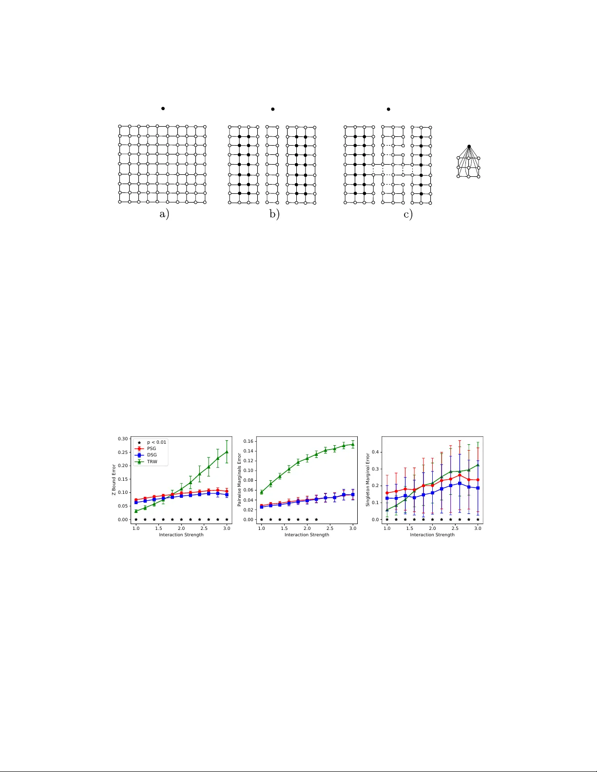
Tract able Minor-free Generaliza tion of Planar Zero-field Ising Models T ractable Minor-free Generalization of Planar Zero-ﬁeld Ising Mo dels V alerii Likhoshersto v vl304@cam.ac.uk Dep artment of Engine ering University of Cambridge Cambridge, UK Y ury Maximo v yur y@lanl.gov The or etic al Division and Center for Nonline ar Studies L os A lamos National L ab or atory L os A lamos, NM, USA Mic hael Chertko v cher tkov@ma th.arizona.edu Gr aduate Pr o gr am in Applie d Mathematics University of A rizona T ucson, AZ, USA Editor: Abstract W e presen t a new family of zero-ﬁeld Ising mo dels o ver N binary v ariables/spins obtained b y consecutive “gluing” of planar and O (1)-sized comp onen ts and subsets of at most three v ertices into a tree. The p olynomial time algorithm of the dynamic programming type for solving exact inference (computing partition function) and exact sampling (generating i.i.d. samples) consists in a sequential application of an eﬃcien t (for planar) or brute-force (for O (1)-sized) inference and sampling to the comp onents as a black b o x. T o illustrate utility of the new family of tractable graphical mo dels, w e ﬁrst build a p olynomial algorithm for inference and sampling of zero-ﬁeld Ising mo dels ov er K 33 -minor-free top ologies and o ver K 5 -minor-free top ologies—both are extensions of the planar zero-ﬁeld Ising mo dels— whic h are neither genus- no treewidth-b ounded. Second, we demonstrate empirically an impro vemen t in the approximation qualit y of the NP-hard problem of inference ov er the square-grid Ising mo del in a no de-dep enden t non-zero “magnetic” ﬁeld. Keyw ords: Graphical mo del, Ising mo del, partition function, statistical inference. 1. In tro duction Let G = ( V ( G ) , E ( G )) b e an undirected graph with a set of v ertices V ( G ) and a set of normal edges E ( G ) ⊆  V ( G ) 2  (no lo ops or multiple edges). W e discuss Ising mo dels whic h asso ciate the following probability to each random N , | V ( G ) | -dimensional binary v ariable/spin conﬁguration X ∈ {± 1 } N : P ( X ) , W ( X ) Z , (1) 1 Likhosherstov, Maximov and Cher tko v where W ( X ) , exp  X v ∈ V ( G ) µ v x v + X e = { v ,w }∈ E ( G ) J e x v x w  and Z , X X ∈{± 1 } N W ( X ) . (2) Here, µ = ( µ v , v ∈ V ( G )) is a vector of (magnetic) ﬁelds , J = ( J e , e ∈ E ( G )) is a vector of the (p airwise) spin inter actions , and the normalization constan t Z , whic h is deﬁned as a sum ov er 2 N spin conﬁgurations, is referred to as the p artition function . Giv en the mo del sp eciﬁcation I = h G, µ, J i , w e address the tasks of ﬁnding the exact v alue of Z (inference) and drawing exact samples with the probabilit y (1). Related w ork. It has b een kno wn since the seminal con tributions of Fisher (1966) and Kasteleyn (1963) that computation of the partition function in the zero-ﬁeld ( µ = 0) Ising mo del ov er a planar graph and sampling from the resp ective probability distribution are b oth tractable, that is, these are tasks of complexity p olynomial in N . As sho wn by Barahona (1982), even when G is planar or when µ = 0 ( zer o ﬁeld ), the p ositiv e results are hard to generalize—b oth addition of the non-zero (magnetic) ﬁeld and the extension b ey ond planar graphs make the computation of the partition function NP-hard. These results are also consis ten t with the statemen t from Jerrum and Sinclair (1993) that computation of the partition function of the zero-ﬁeld Ising mo del is a #P-complete problem, even in the ferromagnetic case when all comp onents of J are p ositiv e. Therefore, describing h G, µ, J i families for whic h computations of the partition function and sampling are tractable remains an op en question. The simplest tractable (i.e., inference and sampling are p olynomial in N ) example is one when G is a tree, and the corresp onding inference algorithm, known as dynamic pr o- gr amming and/or b elief pr op agation , has a long history in physics (Bethe, 1935; P eierls, 1936), optimal control (Bellman, 1952), information theory (Gallager, 1963), and artiﬁcial in telligence (P earl, 1982). Extension to the case when G is a tree of ( t + 1)-sized cliques “glued” together, or more formally when G is of a tr e ewidth t , is known as the junction tr e e algorithm (V erner Jensen et al., 1990), which has complexit y of counting and sampling that gro w exponentially with t . Another insight originates from the foundational statistical physics literature of the last cen tury related to the zero-ﬁeld v ersion of (1), i.e. when µ = 0, ov er planar G . Onsager (1944) found a closed-form solution of (1) in the case of a homogeneous Ising mo del ov er an inﬁnite t w o-dimensional square grid. Kac and W ard (1952) reduced the inference of (1) o v er a ﬁnite square lattice to computing a determinant. Kasteleyn (1963) generalized this result to an arbitrary (ﬁnite) planar graph. Kasteleyn’s approach consists of expanding eac h v ertex of G into a gadget and reducing the Ising mo del inference to the problem of counting p erfect matchings ov er the expanded graph. Kasteleyn’s construction w as simpliﬁed by Fisher (1966). The tigh test running time estimate for Kasteleyn’s metho d giv es O ( N 3 2 ). Kasteleyn conjectured, whic h was later prov en b y Gallucio and Loebl (1999), that the approac h extends to the case of the zero-ﬁeld Ising mo del o ver graphs em b edded in a surface of genus g with a multiplicativ e O (4 g ) p enalty . A parallel w ay of reducing the planar zero-ﬁeld Ising mo del to a perfect matching coun t- ing problem consists of constructing the so-called expanded dual graph (Bieche et al., 1980; Barahona, 1982; Schraudolph and Kamenetsky, 2009). This approach is adv antageous b e- cause using the expanded dual graph allo ws a one-to-one corresp ondence betw een spin 2 Tract able Minor-free Generaliza tion of Planar Zero-field Ising Models conﬁgurations and p erfect matchings. An extra adv antage of this approach is that the re- duction allo ws us to dev elop an exact eﬃcient sampling. Based on linear algebra and planar separator theory (Lipton and T arjan, 1979), Wilson (1997) introduced an algorithm that allo ws to sample perfect matchings o ver planar graphs in O ( N 3 2 ) time. The algorithms w ere implemen ted b y Thomas and Middleton (2009, 2013) for the Is ing mo del sampling, how ever, the implementation was limited to only the sp ecial case of a square lattice. Thomas and Middleton (2009) also suggested a simple extension of the Wilson’s algorithm to the case of b ounded gen us graphs, again with the 4 g factor in complexity . Notice that imp osing the zero ﬁeld condition is critical, as otherwise, the Ising mo del ov er a planar graph is NP-hard (Barahona, 1982). On the other hand, even in the case of zero magnetic ﬁeld the Ising mo dels ov er general graphs are diﬃcult (Barahona, 1982). W agner’s theorem (Diestel, 2006, chap. 4.4) states that G is planar if and only if it do es not ha ve K 33 and K 5 as minors (Figure 2(b)). Both families of K 33 -free and K 5 -free graphs generalize and extend the family of planar graphs, since K 33 ( K 5 ) is nonplanar but K 5 -free ( K 33 -free). Both families are genus-un b ounded, since a disconnected set of g K 33 ( K 5 ) graphs has a gen us of g (Battle et al., 1962) and is K 5 -free ( K 33 -free). Moreov er, b oth families are treewidth-unbounded, since planar square grid of size t × t has a treewidth of t (Bo dlaender, 1998). Therefore, the question of interest b ecomes generalizing tractable inference and sampling in the zero-ﬁeld Ising mo del o ver a K 33 -free or K 5 -free graph. T o extend tractabilit y of the sp ecial cases as an appro ximation to a more general class of inference problems it is natural to consider a family of tractable spanning subgraphs and then exploit the fact that the log-partition function log Z ( µ, J ) is con v ex and hence can b e upp er-bounded b y a linear combination of tractable partition functions. T ree-reweigh ted (TR W) approximation (W ain wrigh t et al., 2005) was the ﬁrst example in the literature where such upp er-bounding was constructed with the trees used as a basic element. The upp er-bound TR W approac h (W ain wright et al., 2005) was extended b y Glob erson and Jaakk ola (2007), where utilizing a planar spanning subgraph (and not a tree) as the basic (tractable) element was suggested. Con tribution. In this man uscript, w e, ﬁrst of all, compile results that w ere scattered o v er the literature on (at least) O ( N 3 2 )-eﬃcien t exact sampling and exact inference in the zero-ﬁeld Ising model o v er planar graphs. T o the b est of our kno wledge, we are the ﬁrst to presen t a complete and mathematically accurate description of the tigh t asymptotic b ounds. Then, we describ e a new family of zero-ﬁeld Ising mo dels on graphs that are more general than planar. Given a tree decomp osition of such graphs into planar and “small” ( O (1)-sized) comp onents “glued” together along sets of at most three v ertices, inference and sampling ov er the new family of mo dels is of p olynomial time. W e further sho w that all the K 33 -free or K 5 -free graphs are included in this family and, moreov er, their aforementioned tree decomposition can b e constructed with O ( N ) eﬀorts. This allo ws us to pro v e an O ( N 3 2 ) upp er b ound on run time complexity for exact inference and exact sampling of the K 5 -free or K 33 -free zero-ﬁeld Ising mo dels. Finally , w e sho w ho w the newly introduced tractable family of the zero-ﬁeld Ising mo dels allo ws extension of the approac h of Glob erson and Jaakkola (2007) resulting in an upp er- b ound for log-partition function ov er general Ising mo dels, non-planar and including non- zero magnetic ﬁeld. Instead of using planar spanning subgraphs as in the w ork of Glob erson and Jaakkola (2007), w e use more general (non-planar) basic tractable elements. Using 3 Likhosherstov, Maximov and Cher tko v the metho dology of Globerson and Jaakkola (2007), we illustrate the approach through exp erimen ts with a nonzero-ﬁeld Ising mo del on a square grid for whic h exact inference is kno wn to b e NP-hard (Barahona, 1982). Relation to other algorithms. The result presented in this manuscript is similar to the approac h used to count p erfect matc hings in K 5 -free graphs (Curticap ean, 2014; Straub et al., 2014). Ho wev er, we do not use a transition to p erfect matching coun ting as it is typically done in studies of zero-ﬁeld Ising mo dels ov er planar graphs (Fisher, 1966; Kasteleyn, 1963; Thomas and Middleton, 2009). Presumably , a direct transition to p erfect matc hing coun ting can b e done via a construction of an expanded graph in the fashion of Fisher (1966); Kasteleyn (1963). How ever, this results in a size increase and, what’s more imp ortan t, there is no direct corresp ondence betw een spin conﬁgurations and p erfect matc hings, therefore exact sampling is not supp orted. Structure. Section 2 states the problems of exact inference and exact sampling for pla- nar zero-ﬁeld Ising mo dels. In Section 3 we in tro duce the concept of c -nice decomposition of graphs, and then formulate and prov e tractability of the zero-ﬁeld Ising mo dels ov er graphs whic h are c -nice decomp osible. Section 4 is devoted to application of the algorithm intro- duced in the preceding Section to examples of the zero-ﬁeld Ising mo del o ver the K 33 -free (but p ossibly K − 5 containing) and K 5 -free (but p ossibly K 3 , 3 con taining) graphs. Section 5 presen ts an empirical application of the newly in tro duced family of tractable models to an upp er-bounding log-partition function of a broader family of intractable graphical mo dels (planar nonzero-ﬁeld Ising mo dels). Section 6 is reserv ed for conclusions. Throughout the text, w e use common graph-theoretic notations and deﬁnitions (Diestel, 2006) and also restate the most important concepts brieﬂy . 2. Planar T op ology In this Section, w e consider the special I = h G, 0 , J i case of the zero-ﬁeld Ising model o v er a planar graph and in tro duce transition from I to the perfect matching model ov er a diﬀerent (deriv ed from G ) planar graph. One-to-one corresp ondence b et ween a spin conﬁguration o v er the Ising mo del and corresp onding p erfect matching conﬁguration ov er the derived graph translates the exact inference and exact sampling o ver I to the corresp onding exact inference and exact sampling in the deriv ed p erfect matc hing mo del. 2.1 Expanded Dual Graph The graph is planar when it can be dra wn on (em b edded in to) a plane without edge in ter- sections. W e assume that the planar embedding of G is given (and if not, it can b e found in O ( N ) time according to Bo yer and Myrv old (2004)). In this Section we follow in our constructions of Schraudolph and Kamenetsky (2009). Let us, ﬁrst, triangulate G by triangulating one after another eac h face of the original graph and then setting J e = 0 for all the newly added edges e ∈ E ( G ). Complexit y of the triangulation is O ( N ), see Schraudolph and Kamenetsky (2009) for an example. (F or con v enience, we will then use the same notation for the derived, triangulated graph as for the original graph.) Second, construct a new graph, G F , where each v ertex f of V ( G F ) is a face of G , and there is an edge e = { f 1 , f 2 } in E ( G F ) if and only if f 1 and f 2 share an edge in G . By 4 Tract able Minor-free Generaliza tion of Planar Zero-field Ising Models (a) + + + + + - (b) Figure 1: (a) A fragment of G ’s em b edding after triangulation (blac k), expanded dual graph G ∗ (red). (b) Possible X conﬁgurations and corresp onding M ( X ) (wa vy lines) on a single face of G . Rotation symmetric and rev erse sign conﬁgurations are omitted. construction, G F is planar, and it is em b edded in the same plane as G , so that each new edge e = { f 1 , f 2 } ∈ E ( G F ) intersects the resp ectiv e old edge. Call G F a dual gr aph of G . Since G is triangulated, each f ∈ V ( G F ) has degree 3 in G F . Third, obtain a planar graph G ∗ and its em b edding from G F b y substituting eac h f ∈ V ( G F ) b y a K 3 triangle so that each vertex of the triangle is incident to one edge, going outside the triangle (see Figure 1(a) for illustration). Call G ∗ the exp ande d dual gr aph of G . Newly introduced triangles of G ∗ , substituting G F ’s vertices, are called Fisher cities (Fisher, 1966). W e refer to edges outside triangles as inter city e dges and denote their set as E ∗ I . The set E ( G ∗ ) \ E ∗ I of Fisher city edges is denoted as E ∗ C . Notice that e ∗ ∈ E ∗ I in tersects exactly one e ∈ E ( G ) and vice versa, which deﬁnes a bijection b et w een E ∗ I and E ( G ); denote it b y g : E ∗ I → E ( G ). Observ e that | E ∗ I | = | E ( G ) | ≤ 3 N − 6, where N is the size (cardinality) of G . A set E 0 ⊆ E ( G ) is called a p erfe ct matching (PM) of G , if edges of E 0 are disjoint and their union equals V . Let PM( G ) denote the set of all P erfect Matc hings (PM) of G . Notice that E ∗ I is a PM of G ∗ , and thus | V ( G ∗ ) | = 2 | E ∗ I | = O ( N ). Since G ∗ is planar, one also ﬁnds that | E ( G ∗ ) | = O ( N ). Constructing G ∗ requires O ( N ) steps. 2.2 P erfect Matching (PM) Mo del F or every spin conﬁguration X ∈ {± 1 } N , let I ( X ) b e a set { e ∈ E ∗ I | g ( e ) = { v , w } , x v = x w } . Each Fisher city is inciden t to an o dd num b er of edges in I ( X ). Thus, I ( X ) can b e uniquely completed to a PM by edges from E ∗ C . Denote the resulting PM by M ( X ) ∈ PM( G ∗ ) (see Figure 1(b) for an illustration). Let C + = { +1 } × {± 1 } N − 1 . Lemma 1 M is a bije ction b etwe en C + and PM ( G ∗ ) . 5 Likhosherstov, Maximov and Cher tko v Deﬁne weigh ts on G ∗ according to ∀ e ∗ ∈ E ( G ∗ ) : c e ∗ , ( exp(2 J g ( e ∗ ) ) , e ∗ ∈ E ∗ I 1 , e ∗ ∈ E ∗ C (3) Lemma 2 F or E 0 ∈ PM ( G ∗ ) holds P ( M ( X ) = E 0 ) = 1 Z ∗ Y e ∗ ∈ E 0 c e ∗ , (4) wher e Z ∗ , X E 0 ∈ PM ( G ∗ ) Y e ∗ ∈ E 0 c e ∗ = 1 2 Z exp   X e ∈ E ( G ) J e   (5) is the p artition function of the PM distribution (PM mo del) deﬁne d by (4). See proofs of the Lemma 1 and Lemma 2 in App endix A. Second transition of (5) reduces the problem of computing Z to computing Z ∗ . F urthermore, only tw o equiprobable spin conﬁgurations X 0 and − X 0 (one of which is in C + ) corresp ond to E 0 , and they can b e reco v ered from E 0 in O ( N ) steps, thus resulting in the statemen t that one samples from I if sampling from (4) is known. The PM mo del can b e deﬁned for an arbitrary graph ˆ G , ˆ N = | V ( ˆ G ) | with p ositive w eigh ts c e , e ∈ E 0 , as a probability distribution ov er ˆ M ∈ PM( ˆ G ): P ( ˆ M ) ∝ Q e ∈ ˆ M c e . Our subsequen t deriv ations are based on the follo wing Theorem 3 Given the PM mo del deﬁne d on planar gr aph ˆ G of size ˆ N with p ositive e dge weights { c e } , one c an ﬁnd its p artition function and sample fr om it in O ( ˆ N 3 2 ) time (steps). Algorithms, constructively proving the theorem, are directly inferred from Wilson (1997); Thomas and Middleton (2009), with minor changes/generalizations. W e describ e the algo- rithms in App endix B. Corollary 4 Exact infer enc e and exact sampling of the PM mo del over G ∗ (and, henc e, zer o-ﬁeld Ising mo del I over the planar gr aph G ) take O ( N 3 2 ) time. 3. c -nice Decomp osition of the T opology W e commence by introducing the concept of c -nice decomp osition of a graph and stating the main result on the tractability of the new family of Ising mo dels in Subsection 3.1. Then we pro ceed building a helpful “conditioning” machinery in Subsection 3.2 and subse- quen tly describing algorithms for the the eﬃcien t exact inference (Subsection 3.3) and exact sampling (Subsection 3.4), therefore proving the aforemen tioned statemen t constructively . 6 Tract able Minor-free Generaliza tion of Planar Zero-field Ising Models 3.1 Decomp osition tree and the k ey result (of the manuscript) W e mainly follow Curticap ean (2014); Reed and Li (2008) in the deﬁnition of the decomp o- sition tree and its prop erties suﬃcient for our goals. (Let us also remind that we consider here graphs containing no self-lo ops or multiple edges.) Graph G 0 is a sub gr aph of G whenever V ( G 0 ) ⊆ V ( G ) and E ( G 0 ) ⊆ E ( G ). F or tw o subgraphs G 0 and G 00 of G , let G 0 ∪ G 00 = ( V ( G 0 ) ∪ V ( G 00 ) , E ( G 0 ) ∪ E ( G 00 )) (graph union ). Consider a tree decomp osition T = h T , G i of a graph G in to a set of subgraphs G , { G t } of G , where t are no des of a tree T , that is, t ∈ V ( T ). One of the no des of the tree, r ∈ V ( T ), is selected as the ro ot. F or eac h no de t ∈ V ( T ), its p ar ent is the ﬁrst no de on the unique path from t to r . G ≤ t denotes the graph union of G t 0 for all the no des t 0 in V ( T ) that are t or its descendants. G  t denotes the graph union of G t 0 for all the no des t 0 in V ( T ) that are neither t nor descendants of t . F or t wo neighboring no des of the tree, t, p ∈ V ( T ) and { t, p } ∈ E ( T ), the set of ov erlapping v ertices of G t and G p , K , V ( G t ) ∩ V ( G p ), is called an attachment set of t or p . If p is a parent of t , then K is a navel of t . W e assume that the nav el of the root is empt y . T is a c -nic e de c omp osition of G if the following requirements are satisﬁed: 1. ∀ t ∈ V ( T ) with a nav el K , it holds that K = V ( G ≤ t ) ∩ V ( G  t ). 2. Every attac hmen t set K is of size 0, 1, 2, or 3. 3. ∀ t ∈ V ( T ), either | V ( G t ) | ≤ c or G t is planar. 4. If t ∈ V ( T ) is such that | V ( G t ) | > c , addition of all edges of type e = { v , w } , where v , w b elong to the same attachmen t set of t (if e is not yet in E ( G t )) do es not destroy planarit y of G t . Stating it informally , the c -nice decomp osition of G is a tree decomp osition of G in to planar and “small” (of size at most c ) subgraphs G t , “glued” via subsets of at most three v ertices of G . Figure 2(a) shows an example of a c -nice decomp osition with c = 8. There are v arious similar w a ys to deﬁne a graph decomp osition in literature, and the one pre- sen ted ab o v e is customized (to our purp oses) to include only prop erties signiﬁcan t for our consecutiv e analysis. The remainder of this Section is dev oted to a constructiv e pro of of the following k ey statemen t of the man uscript. Theorem 5 L et I = h G, 0 , J i b e any zer o-ﬁeld Ising mo del wher e ther e exists a c -nic e de c omp osition T of G , wher e c is an absolute c onstant. Then, ther e is an algorithm which, given I , T as an input: (1) ﬁnds Z and (2) samples a c onﬁgur ation fr om I in time O ( P t ∈ V ( T ) | V ( G t ) | 3 2 ) . 3.2 Inference and sampling conditioned on 1, 2, or 3 vertices/spins Before presenting the algorithm that prov es Theorem 5 constructively , let us introduce the auxiliary machinery of “conditioning”, which describ es the partition function of a zero-ﬁeld Ising mo del ov er a planar graph conditioned on 1, 2, or 3 spins. Consider a zero-ﬁeld Ising 7 Likhosherstov, Maximov and Cher tko v + + – + Figure 2: a) An exemplary graph G and its 8-nice decomp osition T , where t ∈ { 1 , · · · , 7 } lab els nodes of the decomp osition tree T and no de 4 is c hosen as the ro ot ( r = 4). Iden tical v ertices of G in its subgraphs G t are sho wn connected b y dashed lines. Na v els of size 1, 2, and 3 are highlighted. Component G 5 is nonplanar, and G 4 b ecomes nonplanar when all attac hmen t edges are added (according to the fourth item of the deﬁnition of the c -nice decomp osition). G ≤ 3 and G  3 are shown with dotted lines. Note that the decomp osition is non-unique for the graph. F or instance, edges that belong to the attachmen t set can go to either of the t w o subgraphs containing this set or even rep eat in b oth. b) Minors K 5 and K 33 are forbidden in the planar graphs. M¨ obius ladder and its subgraphs are the only nonplanar graphs allow ed in the 8-nice decomp osition of a K 5 -free graph. c) The left panel is an example of conditioning on three vertices/spins in the center of a graph. The right panel shows a mo diﬁed graph where the three vertices (from the left panel) are reduced to one vertex, then leading to a mo diﬁcation of the pairwise in teractions within the associated zero-ﬁeld Ising mo del o ver the reduced graph. d) Example of a graph that con tains K 5 as a minor: b y contracting the highligh ted groups of vertices and deleting the remaining v ertices, one arriv es at the K 5 graph. mo del I = h G, 0 , J i deﬁned ov er a planar graph G . W e intend to use the algorithm for eﬃcien t inference and sampling of I as a black b o x in our subsequent deriv ations. Let us no w in tro duce the notion of c onditioning . Consider a spin conﬁguration X ∈ {± 1 } N , a subset V 0 = { v (1) , . . . , v ( ω ) } ⊆ V ( G ), and deﬁne a c ondition S = { x v (1) = s (1) , . . . , x v ( ω ) = s ( ω ) } on V 0 , where s (1) , . . . , s ( ω ) = ± 1 are ﬁxed v alues. Conditional v ersions of the probability distribution (1 – 2) and the c onditional partition function become P ( X | S ) , W ( X ) × 1 ( X | S ) Z | S , 1 ( X | S ) ,  1 , x v (1) = s (1) , . . . , x v ( ω ) = s ( ω ) 0 , otherwise , (6) where Z | S , X X ∈{± 1 } N W ( X ) × 1 ( X | S ) . (7) 8 Tract able Minor-free Generaliza tion of Planar Zero-field Ising Models Notice that when ω = 0, S = {} and (6 – 7) is reduced to (1 – 2). The subset of V ( G ) is c onne cte d whenev er the subgraph, induced b y this subset is connected. Inference and sampling of I can b e extended as follows (a formal pro of can b e found in the App endix A). Lemma 6 Given I = h G, 0 , J i wher e G is planar and a c ondition S on a c onne cte d subset V 0 ⊆ V ( G ) , | V 0 | ≤ 3 , c omputing the c onditional p artition function Z | S and sampling fr om P ( X | S ) ar e tasks of O ( N 3 2 ) c omplexity. In tuitiv ely , the conditioning algorithm proving the Lemma tak es the subset of connected v ertices and “collapses” them into a single vertex. The graph remains planar and the task is reduced to conditioning on one v ertex, whic h is an elemen tary operation giv en the algorithm from section 2. (See Figure 2(c) for an illustration.) 3.3 Inference algorithm This subsection constructively prov es the inference part of Theorem 5. F or eac h t ∈ V ( T ), let I ≤ t , h G ≤ t , 0 , { J e | e ∈ E ( G ≤ t ) ⊆ E ( G ) }i denote a zero-ﬁeld Ising submo del induc e d b y G ≤ t . Denote the partition function and subv ector of X related to I ≤ t as Z ≤ t and X ≤ t , { x v | v ∈ V ( G ≤ t ) } , resp ectively . F urther, let K b e t ’s nav el and let S = {∀ v ∈ K : x v = s ( v ) } denote some condition on K . Recall that | K | ≤ 3. F or each t , the algorithm computes conditional partition functions Z ≤ t | S for all c hoices of condition spin v alues { s ( v ) = ± 1 } . Each t is pro cessed only when its c hildren ha ve already b een pro cessed, so the algorithm starts at the leaf and ends at the ro ot. If r ∈ G ( T ) is a ro ot, its na vel is empty and G ≤ r = G , hence Z = Z ≤ r |{} is computed after r ’s pro cessing. Supp ose all c hildren of t , c 1 , ..., c m ∈ V ( T ) with na v els K 1 , ..., K m ⊆ V ( G t ) ha ve already b een pro cessed, and now t itself is considered. Denote a spin conﬁguration on G t as Y t , { y v = ± 1 | v ∈ V ( G t ) } . I ≤ c 1 , ..., I ≤ c m are I ≤ t ’s submo dels induced by G ≤ c 1 , ..., G ≤ c m , which can only in tersect at their nav els in G t . Based on this, one states the following dynamic programming relation: Z ≤ t | S = X Y t ∈{± 1 } | V ( G t ) | 1 ( Y t | S ) exp   X e = { v ,w }∈ E ( G t ) J e y v y w   · m Y i =1 Z ≤ c i | S i [ Y t ] . (8) Here, S i [ Y t ] denotes a condition {∀ v ∈ K i : x v = y v } on K i . The goal is to eﬃciently p erform summation in (8). Let I (0) , I (1) , I (2) , I (3) b e a partition of { 1 , ..., m } by nav el sizes. Figure 3(a,b) illustrates inference in t . 1. Na v els of size 0, 1. Notice that if i ∈ I (0) , then Z ≤ c i |{} = Z ≤ c i is constant, which was computed b efore. The same is true for i ∈ I (1) and Z ≤ c i | S ( i ) [ Y t ] = 1 2 Z ≤ c i . 2. Na v els of size 2. Let i ∈ I (2) denote K i = { u i , q i } and simplify notation Z ≤ c i y 1 ,y 2 , Z ≤ c i x u i = y 1 ,x q i = y 2 for conv enience. Notice that Z ≤ c i | S i [ Y t ] is strictly p ositiv e, and due to the zero-ﬁeld nature of I ≤ c i , one ﬁnds Z ≤ c i | +1 , +1 = Z ≤ c i |− 1 , − 1 and Z ≤ c i | +1 , − 1 = Z ≤ c i |− 1 , +1 . Then, one arrives at log Z ≤ c i | S i [ Y t ] = A i + B i y u i y q i , where A i , log Z ≤ c i | +1 , +1 + log Z ≤ c i | +1 , − 1 and B i , log Z ≤ c i | +1 , +1 − log Z ≤ c i | +1 , − 1 . 9 Likhosherstov, Maximov and Cher tko v + – + + – + + – – + – – + + – + + – Figure 3: a) Example of inference at no de t with children c 1 , c 2 , c 3 , c 4 . Na v els K 1 = { u 1 , q 1 , h 1 } , K 2 = { u 2 , q 2 , h 2 } , K 3 = { u 2 , q 2 } , K 4 = { u 4 } , and K = { u, q , h } are highlighted. F ragmen ts of I ≤ c i are shown with dotted lines. Here, I (0) = ∅ , I (1) = { 4 } , I (2) = { 3 } , and I (3) = { 1 , 2 } , indicating that one child is glued ov er one no de, one child is glued o v er tw o no des, and tw o children are glued o ver three no des. b) “Aggregated” Ising mo del I t and its pairwise in teractions are shown. Both c) and d) illustrate sampling ov er I t . One sample spins in I t conditioned on S ( t ) and then rep eats the pro cedure at the child no des. 3. Na v els of size 3. Let i ∈ I (3) , and as ab o ve, denote K i = { u i , q i , h i } and Z ≤ c i y 1 ,y 2 ,y 3 , Z ≤ c i x u i = y 1 ,x q i = y 2 ,x h i = y 3 . Due to the zero-ﬁeld nature of I ≤ c i , it holds that Z ≤ c i | +1 ,y 2 ,y 3 = Z ≤ c i |− 1 ,y 2 ,y 3 . Observe that there are suc h A i , B i , C i , D i that log Z ≤ c i | y 1 ,y 2 ,y 3 = A i + B i y 1 y 2 + C i y 1 y 3 + D i y 2 y 3 for all y 1 , y 2 , y 3 = ± 1, whic h is guaranteed since the following system of equations has a solution:       log Z ≤ c i | +1 , +1 , +1 log Z ≤ c i | +1 , +1 , − 1 log Z ≤ c i | +1 , − 1 , +1 log Z ≤ c i | +1 , − 1 , − 1       =     +1 +1 +1 +1 +1 +1 − 1 − 1 +1 − 1 +1 − 1 +1 − 1 − 1 +1     ×     A i B i C i D i     . (9) Considering three cases, one rewrites Eq. (8) as Z ≤ t | S = M · X Y t 1 ( Y t | S ) exp  X e = { v ,w }∈ E ( G t ) J e y v y w + X i ∈ I (2) ∪ I (3) B i y u i y q i + X i ∈ I (3) ( C i y u i y h i + D i y q i y h i )  , (10) where M , 2 −| I (1) | ·  Q i ∈ I (0) ∪ I (1) Z ≤ c i  · exp( P i ∈ I (2) ∪ I (3) A i ). The sum in Eq. (10) is simply a conditional partition function of a zero-ﬁeld Ising mo del I t deﬁned ov er a graph G t with pairwise in teractions of I adjusted by the addition of B i , C i , and D i summands at the appropriate nav el edges (if a corresp onding edge is not present in G t , it has to b e added). If | V ( G t ) | ≤ c , then (10) is computed a maximum of four times (dep ending on nav el size) b y brute force ( O (1) time). Otherwise, if K is a disconnected set in G t , w e add zero-in teraction 10 Tract able Minor-free Generaliza tion of Planar Zero-field Ising Models edges inside it to make it connected. P ossible addition of edges inside K, K 1 , . . . , K m do esn’t destro y planarity according to the fourth item in the deﬁnition of the c -nice decomp osition ab o ve. Finally , w e compute (10) using Lemma 6 in time O ( | V ( G t ) | 3 2 ). The inference part of Theorem 5 follo ws directly from the pro cedure just describ ed. 3.4 Sampling al gorithm Next, w e address the sampling part of Theorem 5. W e extend the algorithm from section 3.3 so that it supp orts eﬃcient sampling from I . Assume that the inference pass through T (from leav es to ro ot) has b een done so that I t for all t ∈ V ( T ) are computed. Denote X t , { x v | v ∈ V ( G t ) } . The sampling algorithm runs backw ards, ﬁrst drawing spin v alues X r at the root r of T from the marginal distribution P ( X r ), and then processing eac h no de t of T after its parent p is pro cessed. Pro cessing consists of dra wing spins X t from P ( X t | X p ) = P ( X t | X ( t ) , { x v | v ∈ K } ), where K is a nav el of t . This marginal-conditional sc heme generates the correct sample X of spins ov er G . Let P ≤ t ( X ≤ t ) deﬁne a spin distribution of I ≤ t . Because the Ising mo del is an example of Marko v Random Field, it holds that P ≤ t ( X ≤ t | X ( t ) ) = P ( X ≤ t | X ( t ) ). W e further deriv e P ( X t | X ( t ) ) = P ≤ t ( X t | X ( t ) ) = 1 Z ≤ t X X ≤ t \ X t exp  X e = { v ,w }∈ E ( G ≤ t ) J e x v x w  = 1 Z ≤ t · exp  X e = { v ,w }∈ E ( G t ) J e x v x w  · m Y i =1 Z ≤ c i | S i [ X t ] ∝ exp  X e = { v ,w }∈ E ( G t ) J e x v x w + X i ∈ I (2) ∪ I (3) B i x u i x q i + X i ∈ I (3) ( C i x u i x h i + D i x q i x h i )  . (11) In other words, sampling from P ( X t | X ( t ) ) is reduced to sampling from I t conditional on spins X ( t ) in the nav el K . It is done via brute force if | V ( G t ) | ≤ c ; otherwise, Lemma 6 allo ws one to draw X t in O ( | V ( G t ) | 3 2 ), since | K | ≤ 3. Sampling eﬀorts cost as muc h as inference, which concludes the proof of Theorem 5. Figure 3(c,d) illustrates sampling in t . 4. Minor-free Extension of Planar Zero-ﬁeld Ising Mo dels Contr action is an operation of remo ving tw o adjacen t vertices v and u (and all edges inciden t to them) from the graph and adding a new vertex w adjacent to all neighbors of v and u . F or tw o graphs G and H , H is G ’s minor , if it is isomorphic to a graph obtained from G ’s subgraph by a series of contractions (Figure 2(d)). G is H -fr e e , if H is not G ’s minor. According to W agner’s theorem (Diestel, 2006, chap. 4.4), a set of planar graphs coin- cides with an intersection of K 33 -free graphs and K 5 -free graphs. Some nonplanar graphs are K 33 -free ( K 5 -free), for example, K 5 ( K 33 ). K 33 -free ( K 5 -free) graphs are neither gen us- b ounded (a disconnected set of g K 5 ( K 33 ) graphs is K 33 -free ( K 5 -free) and has a genus of g (Battle et al., 1962)). K 33 -free ( K 5 -free) graphs are treewidth-un b ounded as well (planar square grid of size t × t is K 33 -free and K 5 -free and has a treewidth of t (Bodlaender, 1998)). In the remainder of the section w e show that a c -nice decomp osition of K 33 -free graphs and K 5 -free graphs can b e computed in p olynomial time and, hence, inference and sampling of zero-ﬁeld Ising mo dels on these graph families can be p erformed eﬃciently . 11 Likhosherstov, Maximov and Cher tko v 4.1 Zero-ﬁeld Ising Mo dels ov er K 33 -free Graphs Ev en though K 33 -free graphs are Pfaﬃan-orientable (with the Pfaﬃan orientation com- putable in p olynomial time, see V azirani (1989)), the expanded dual graph—in tro duced to map the zero-ﬁeld Ising mo del to the resp ectiv e PM problem—is not necessarily K 33 - free. Therefore, the latter is generally not Pfaﬃan-orien table. Hence, the reduction to a w ell-studied perfect matching coun ting problem is not straigh tforward. Theorem 7 L et G b e K 33 -fr e e gr aph of size N with no lo ops or multiple e dges. Then the 5 -nic e de c omp osition T of G exists and c an b e c ompute d in time O ( N ) . Pro of (Sk etch) An equiv alent decomp osition is constructed by Hopcroft and T arjan (1973); Gut w enger and Mutzel (2001); V o (1983) in time O ( N ). W e put a formal pro of into Ap- p endix C. Remark 8 The O ( N ) c onstruction time of T guar ante es that P t ∈ V ( T ) | V ( G t ) | = O ( N ) . A l l nonplanar c omp onents in T ar e isomorphic to K 5 or its sub gr aph. Therefore, if G is K 33 -free, it satisﬁes all the conditions needed for eﬃcient inference and sampling, describ ed in section 3. Theorem 9 F or any I = h G, 0 , J i wher e G is K 33 -fr e e, infer enc e or sampling of I takes O ( N 3 2 ) steps. Pro of Finding 5-nice T for G is the O ( N ) op eration. Pro vided with T , inference and sampling take at most O   X t ∈ V ( T ) | V ( G t ) | 3 2   = O      X t ∈ V ( T ) | V ( G t ) |   3 2    = O ( N 3 2 ) (12) where we apply con vexit y of f ( z ) = z 3 2 and the Remark after Theorem 7. 4.2 K 33 -free Zero-ﬁeld Ising Mo dels: Implemen tation and T ests In addition to theoretical justiﬁcation, which is fully presen ted in this man uscript, w e per- form emprical sim ulations to v alidate correctness of inference and sampling algorithm for K 33 -free zero-ﬁeld Ising mo dels. T o test the correctness of inference, w e generate random K 33 -free mo dels of a giv en size and then compare the v alue of PF computed in a brute force wa y (tractable for suﬃcien tly small graphs) and by our algorithm. See the graph generation algorithm in Appe ndix E. W e sim ulate samples of sizes from { 10 , ..., 15 } (1000 samples p er size) and verify that resp ectiv e expressions coincide. When testing sampling implementation, we take for granted that the pro duced samples do not correlate given that the sampling pro cedure accepts the Ising mo del as input and 12 Tract able Minor-free Generaliza tion of Planar Zero-field Ising Models 2 4 6 8 10 l o g 2 m 0 5 10 15 20 25 30 K L - d i v e r g e n c e N=10 N=25 N=40 (a) 3 4 5 6 7 8 9 10 l og 2 N 10 8 6 4 2 0 2 4 6 l o g 2 ( s e c . ) C * N 1.5 infere nce s am pli ng (b) Figure 4: (a) KL-divergence of the mo del probability distribution compared with the em- pirical probabilit y distribution. N , m are the mo del’s size and the n umber of samples, resp ectiv ely . (b) Execution time of inference (red dots) and sampling (blue dots) dep ending on N , shown on a logarithmic scale. Black line corresp onds to O ( N 3 2 ). uses indep enden t random num b er generator inside. The construction do es not ha ve any memory , therefore, it generates statistically indep enden t samples. T o test that the em- pirical distribution is approaching a theoretical one (in the limit of the inﬁnite num b er of samples), we dra w diﬀeren t n um b ers m of samples from a mo del of size N . Then we ﬁnd Kullbac k-Leibler div ergence b et ween the probability distribution of the mo del (here we use our inference algorithm to compute the normalization, Z ) and the empirical probability , obtained from samples. Fig. 4(a) shows that KL-divergence con verges to zero as the sample size increases. Zero KL-div ergence corresponds to equal distributions. Finally , we simulate inference and sampling for random mo dels of diﬀerent size N and observ e that the computational time (eﬀorts) scales as O ( N 3 2 ) (Figure 4(b)). 1 4.3 Zero-ﬁeld Ising Mo dels ov er K 5 -free Graphs It can b e shown that result similar to the one describ ed abov e for the K 33 -free graphs also holds for the K 5 -free graphs as w ell. Theorem 10 L et G b e a K 5 -fr e e gr aph of size N with no lo ops or multiple e dges. Then, the 8 -nic e de c omp osition T of G exists and c an b e c ompute d in time O ( N ) . Pro of (Sketc h) An equiv alent decomp osition is constructed by Reed and Li (2008) in time O ( N ). See App endix D for formal pro of. Remark 11 The O ( N ) c onstruction time of T guar ante es that P t ∈ V ( T ) | V ( G t ) | = O ( N ) . A l l nonplanar c omp onents in T ar e isomorphic to the M¨ obius ladder (Figur e 2(b)) or its sub gr aph. 1. Implementation of the algorithms is a v ailable at h ttps://github.com/V aleryT yumen/planar ising. 13 Likhosherstov, Maximov and Cher tko v The graph in Figure 2(a) is actually K 5 -free. Theorems 5 and 10 allow us to conclude: Theorem 12 Given I = h G, 0 , J i with K 5 -fr e e G of size N , ﬁnding Z and sampling fr om I take O ( N 3 2 ) total time. Pro of Analogous to the pro of of Theorem 9. 5. Appro ximate Inference of Square-grid Ising Mo del In this section, we consider I = h G, µ, J i such that G is a square-grid graph of size H × H . Finding Z ( G, µ, J ) for arbitrary µ , J is an NP-hard problem (Barahona, 1982) in such a setting. Construct G 0 b y adding an ap ex vertex connected to all G ’s vertices by edge (Figure 5(a)). Now it can easily b e seen that Z ( G, µ, J ) = 1 2 Z ( G 0 , 0 , J 0 = ( J µ ∪ J )), where J µ = µ are interactions assigned for ap ex edges. Let { G ( r ) } b e a family of spanning graphs ( V ( G ( r ) ) = V ( G 0 ), E ( G ( r ) ) ⊆ E ( G 0 )) and J ( r ) b e in teraction v alues on G ( r ) . Also, denote ˆ J ( r ) = J ( r ) ∪ { 0 , e ∈ E ( G 0 ) \ E ( G ( r ) ) } . Assuming that log Z ( G ( r ) , 0 , J ( r ) ) are tractable, the con v exity of log Z ( G 0 , 0 , J 0 ) allo ws one to write the follo wing upp er b ound: log Z ( G 0 , 0 , J 0 ) ≤ min ρ ( r ) ≥ 0 , P r ρ ( r )=1 { J ( r ) } , P r ρ ( r ) ˆ J ( r ) = J 0 X r ρ ( r ) log Z ( G ( r ) , 0 , J ( r ) ) . (13) After graph set { G ( r ) } has b een ﬁxed, one can n umerically optimize the right-hand side of (13), as shown in Glob erson and Jaakkola (2007) for planar G ( r ) . The extension of the basic planar case is straigh tforw ard and is detailed in the App endix F. The App endix also con tains description of marginal probabilities appro ximation suggested in Glob erson and Jaakk ola (2007); W ainwrigh t et al. (2005). The choice for a planar spanning graph (PSG) family { G ( r ) } of Glob erson and Jaakk ola (2007) is illustrated in Figure 5(b). A tractable decomp osition-based extension of the planar case presen ted in this man uscript suggests a more adv anced construction—decomp osition- based spanning graphs (DSG) (Figure 5(c)). W e compare p erformance of b oth PSG and DSG approac hes as well as the performance of tree-rew eighted approximation (TR W) (W ain- wrigh t et al., 2005) in the follo wing setting of V arying Inter action : µ ∼ U ( − 0 . 5 , 0 . 5), J ∼ U ( − α, α ), where α ∈ { 1 , 1 . 2 , 1 . 4 , . . . , 3 } . W e opt optimize for grid size H = 15 (225 v ertices, 420 edges) and compare upp er b ounds and marginal probability approximations (sup erscript alg ) with exact v alues obtained using a junction tree algorithm (V erner Jensen et al., 1990) (sup erscript true ). W e compute three types of error: 1. normalized log-partition error 1 H 2 (log Z alg − log Z true ), 2. error in pairwise marginals 1 | E ( G ) | P e = { v ,w }∈ E ( G ) | P alg ( x v x w = 1) − P true ( x v x w = 1) | , and 3. error in singleton central marginal | P alg ( x v = 1) − P true ( x v = 1) | where v is a v ertex of G with co ordinates (8 , 8). 14 Tract able Minor-free Generaliza tion of Planar Zero-field Ising Models W e av erage results ov er 100 trials (see Fig. 6). 2 3 W e use the same quasi-Newton algo- rithm (Bertsek as, 1999) and parameters when optimizing (13) for PSG and DSG, but for most settings, DSG outp erforms PSG and TR W. Cases with smaller TR W error can b e explained by the fact that TR W implicitly optimizes (13) ov er the family of al l spanning trees which can b e exp onentially big in size, while for PSG and DSG we only use O ( H ) spanning graphs. Because PSG and DSG approac hes come close to eac h other, w e additionally test for eac h v alue of α on eac h plot, whether the diﬀerence er r P S G − er r DS G is bigger than zero. W e apply a one-sided Wilcoxon’s test (Wilcoxon, 1945) together with the Bonferroni cor- rection b ecause we test 33 times (Jean Dunn, 1961). In most settings, the impro v ement is statistically signiﬁcant (Figure 6). 6. Conclusion In this man uscript, w e, ﬁrst of all, describ e an algorithm for O ( N 3 2 ) inference and sampling of planar zero-ﬁeld Ising mo dels on N spins. Then w e in tro duce a new family of zero-ﬁeld Ising mo dels comp osed of planar components and graphs of O (1) size. F or these mo dels, we describ e a p olynomial algorithm for exact inference and sampling pro vided that the decom- p osition tree is also in the input. A theoretical application is O ( N 3 2 ) inference and sampling algorithm for K 33 -free or K 5 -free zero-ﬁeld Ising models— b oth families are supersets of the family of planar zero-ﬁeld mo dels, and they are b oth neither treewidth- nor gen us-b ounded. W e sho w that our sc heme oﬀers an impro vemen t of the appro ximate inference scheme for ar- bitrary top ologies. The suggested improv ement is based on the planar spanning graph ideas from Glob erson and Jaakk ola (2007) but we use tractable spanning decomp osition-based graphs instead of planar graphs. (That is we k eep the algorithm of Glob erson and Jaakk ola (2007), but substitute planar graphs with a family of spanning decomp osition-based graphs that are tractable.) This improv ement of Globerson and Jaakk ola (2007) results in a tigh ter upp er b ound on the true partition function and a more precise approximation of marginal probabilities. 2. Hardware used: 24-core Intel R  Xeon R  Gold 6136 CPU @ 3.00 GHz 3. Implementation of the algorithms is a v ailable at https://github.com/ValeryTyumen/planar_ising 15 Likhosherstov, Maximov and Cher tko v Figure 5: Construction of graphs used for appro ximate inference on a rectangular lattice. F or b etter visualization, vertices connected to an ap ex are colored white. a) G 0 graph. b) One of planar G ( r ) graphs used in Glob erson and Jaakk ola (2007). Such “separator” pattern is rep eated for eac h column and row, resulting in 2( H − 1) graphs in { G ( r ) } . In addition, Glob erson and Jaakk ola (2007) adds an indep endent variables graph where only ap ex edges are drawn. c) A mo diﬁed “separator” pattern we prop ose. Again, the pattern is rep eated horizontally and vertically resulting in 2( H − 2) graphs + indep endent v ariables graph. This pattern cov ers more magnetic ﬁelds and connects separated parts. Dashed edges indicate the structure of 10-nice decomp osition used for inference. (Nonplanar no de of size 10 is illustrated on the right.) 1.0 1.5 2.0 2.5 3.0 Interaction Strength 0.00 0.05 0.10 0.15 0.20 0.25 0.30 Z Bound Error p < 0.01 PSG DSG TRW 1.0 1.5 2.0 2.5 3.0 Interaction Strength 0.00 0.02 0.04 0.06 0.08 0.10 0.12 0.14 0.16 Pairwise Marginals Error 1.0 1.5 2.0 2.5 3.0 Interaction Strength 0.0 0.1 0.2 0.3 0.4 Singleton Marginal Error Figure 6: Comparison of tree-rew eighted appro ximation (TR W), planar spanning graph (PSG), and decomp osition-based spanning graph (DSG) approaches. The ﬁrst plot is for normalized log-partition error, the second is for error in pairwise marginals, and the third is for error in singleton central marginal. Standard errors o v er 100 trials are shown as error bars. An asterisk “*” indicates the sta- tistically signiﬁcant impro vemen t of DSG ov er PSG, with a p-v alue smaller than 0 . 01 according to the Wilcoxon test with the Bonferroni correction (Wilco xon, 1945). 16 Tract able Minor-free Generaliza tion of Planar Zero-field Ising Models App endix A. Lemma Pro ofs A.1 Lemma 1 Pro of Let E 0 ∈ PM( G ∗ ). Call e ∈ E satur ate d , if it in tersects an edge from E 0 ∩ E ∗ I . Each Fisher cit y is incident to an o dd num b er of edges in E 0 ∩ E ∗ I . Th us, eac h face of G has an ev en n umber of unsaturated edges. This prop erty is preserv ed, when tw o faces/cycles are merged in to one by ev aluating resp ectiv e symmetric diﬀerence. Therefore, one gets that an y cycle in G has an ev en n umber of unsaturated edges. F or each i deﬁne x i := − 1 r i , where r i is the num b er of unsaturated edges on the path connecting v 1 and v i . The deﬁnition is consistent due to aforemen tioned cycle prop ert y . No w for each e = { v , w } ∈ E ( G ), x v = x w if and only if e is saturated. T o conclude, we constructed X suc h that E 0 = M ( X ). Such X is unique, b ecause parit y of unsaturated edges on a path b et ween v 1 and v i uniquely determines relationship b etw een x 1 and x i , and x 1 is alwa ys +1. A.2 Lemma 2 Pro of Let X 0 = ( x 0 1 , ..., x 0 N ) ∈ C + , M ( X 0 ) = E 0 . The statemen t is justiﬁed b y the follo wing c hain of transitions: P ( M ( S ) = E 0 ) = P ( S = X 0 ) + P ( S = − X 0 ) = 2 Z exp   X e = { v ,w }∈ E ( G ) J e x 0 v x 0 w   = 2 Z exp   X e ∗ ∈ E 0 ∩ E ∗ I 2 J g ( e ∗ ) − X e ∈ E ( G ) J e   = 2 Z exp   − X e ∈ E ( G ) J e   Y e ∗ ∈ E 0 ∩ E ∗ I c e ∗ = 2 Z exp   − X e ∈ E ( G ) J e   Y e ∗ ∈ E 0 c e ∗ = 1 Z ∗ Y e ∗ ∈ E 0 c e ∗ (14) A.3 Lemma 6 Pro of W e consider cases depending on ω and consequen tly reduce eac h case to a simpler one. F or conv enience in cases where applies we denote u , v (1) , h , v (2) , q , v (3) : 1. Conditioning on ω = 0 spins. T rivial given the algorithm describ ed in section 2. 17 Likhosherstov, Maximov and Cher tko v 2. Conditioning on ω = 1 spin. Since conﬁgurations X and − X hav e the same probabilit y in I , one deduces that Z | x u = s (1) = 1 2 Z . One also deduces that sampling X from P ( X | x u = s (1) ) is reduced to 1) dra wing X = { x v = ± 1 } from P ( X ) and then 2) returning X = ( s (1) x u ) · X as a result. 3. Conditioning on ω = 2 spins. There is an edge e 0 = { u, h } ∈ E ( G ). The following expansion holds: Z | x u = s (1) ,x h = s (2) = X X, x u = s (1) , x h = s (2) exp  X e = { v ,w }∈ E ( G ) J e x v x w  = exp( J e 0 s (1) s (2) ) · X X, x u = s (1) , x h = s (2) exp  X e = { v ,w }∈ E ( G ) e 6 = e 0 J e x v x w  = exp( J e 0 s (1) s (2) ) · X X, x u = s (1) , x h = s (2) exp  X e = { v ,w }∈ E ( G ) e ∩ e 0 = ∅ J e x v x w + X e = { u,v }∈ E ( G ) v 6 = h ( J e s (1) ) x v · 1 + X e = { h,v }∈ E ( G ) v 6 = u ( J e s (2) ) x v · 1  (15) Obtain graph G 0 from G by con tracting u, h into z . G 0 is still planar and has N − 1 v ertices. Preserve pairwise interactions of edges which were not deleted after contrac- tion. F or each edge e = { u, v } , v 6 = h set J { z ,v } = J e s (1) , for each edge e = { h, v } , v 6 = u set J { z ,v } = J e s (2) . Collapse double edges in G 0 whic h were p ossibly created by transforming in to single edges. A pairwise interaction of the result edge is set to the sum of collapsed in teractions. Deﬁne a zero-ﬁeld Ising mo del I 0 on the resulted graph G 0 with its pairwise in ter- actions, inducing a distribution P 0 ( X 0 = { x 0 v = ± 1 | v ∈ V ( G 0 ) } ). Let Z 0 denote I 0 ’s partition function. A closer lo ok at (15) reveals that Z | x u = s (1) ,x h = s (2) = exp( J e 0 s (1) s (2) ) · Z 0 | x 0 z =1 (16) where Z 0 | z 0 y =1 is a partition function conditioned on a single spin and can b e found eﬃcien tly as shown ab o ve. Since the equality of sums (16) holds summand-wise, for a giv en X 00 = { x 00 v = ± 1 | v ∈ V ( G ) \ { u, h }} the probabilities P ( X 00 ∪ { x u = s (1) , x h = s (2) } | x u = s (1) , x h = s (2) ) and P 0 ( X 00 ∪ { x 0 z = 1 } | x 0 z = 1) are the same. Hence, sampling from P ( X | x u = s (1) , x h = s (2) ) is reduced to conditional sampling from planar zero-ﬁeld Ising mo del P 0 ( X 0 | x 0 z = 1) of size N − 1. 4. Conditioning on w = 3 spins. Without loss of generality assume that u, h are connected b y an edge e 0 in G . A deriv ation similar to (15) and (16) rev eals that (preserving the notation of Case 2) Z | x u = s (1) ,x h = s (2) ,x q = s (3) = exp( J e 0 s (1) s (2) ) · Z 0 | x 0 z =1 ,x 0 q = s (3) (17) 18 Tract able Minor-free Generaliza tion of Planar Zero-field Ising Models whic h reduces inference conditional on 3 vertices to a simpler case of 2 v ertices. Again, sampling from P ( X | x u = s (1) , x t = s (2) , x q = s (3) ) is reduced to a more basic sampling from P 0 ( X 0 | x 0 z = 1 , x 0 q = s (3) ). In principle, Lemma 6 can b e extended to arbitrarily large ω leaving a certain freedom for the Ising mo del conditioning framework. Ho w ev er, in this manuscript we fo cus on a given sp ecial case whic h is enough for our goals. App endix B. Theorem 3 Pro of B.1 Coun ting PMs of Planar ˆ G in O ( ˆ N 3 2 ) time This section addresses inference part of Theorem 3. B.1.1 Pf affian Orient a tion Consider an orien tation on ˆ G . ˆ G ’s cycle of ev en length (built on an even n umber of v ertices) is said to b e o dd-oriente d , if, when all edges along the cycle are tra v ersed in an y direction, an o dd num b er of edges are directed along the trav ersal. F or X ⊆ V ( ˆ G ) let ˆ G ( X ) denote a graph ( X , { e ∈ E ( ˆ G ) | e ⊆ X } ). An orientation of ˆ G is called Pfaﬃan , if all cycles C , such that PM( ˆ G ( V ( ˆ G ) − C )) 6 = ∅ , are o dd-oriented. W e will need ˆ G to contain a Pfaﬃan orientation, moreo ver the construction is easy . Theorem 13 Pfaﬃan orientation of ˆ G c an b e c onstructe d in O ( ˆ N ) . Pro of This theorem is prov en constructively , see e.g. Wilson (1997); V azirani (1989), or Sc hraudolph and Kamenetsky (2009), where the latter construction is based on sp eciﬁcs of the expanded dual graph. Construct a sk ew-symmetric sparse matrix K ∈ R ˆ N × ˆ N ( → denotes orien tation of edges): K ij =      c e if { v i , v j } ∈ E ( ˆ G ) , v i → v j − c e if { v i , v j } ∈ E ( ˆ G ) , v j → v i 0 if { v i , v j } / ∈ E ( ˆ G ) (18) The next result allo ws to compute PF ˆ Z of PM mo del on ˆ G in a p olynomial time. Theorem 14 det K > 0 , ˆ Z = √ det K . Pro of See, e.g., Wilson (1997) or Kasteleyn (1963). B.1.2 Computing det K LU-decomp osition of a matrix A = LU , found via Gaussian elimination, where L is a low er- triangular matrix with unit diagonals and U is an upp er-triangular matrix, would b e a 19 Likhosherstov, Maximov and Cher tko v standard w ay of computing det A , which is then equal to a product of the diagonal elements of U . Ho w ev er, this standard w a y of constructing the LU decomp osition applies only if all A ’s leading principal submatrices are nonsingular (See e.g. Horn and Johnson (2012), section 3.5, for detailed discussions). And already the 1 × 1 leading principal submatrix of K is zero/singular. Luc kily , this diﬃculty can b e resolv ed through the follo wing construction. T ake ˆ G ’s arbitrary p erfect matching E 0 ∈ PM( ˆ G ). In the case of a general planar graph E 0 can b e found via e.g. Blum’s algorithm (Blum, 1990) in O ( p ˆ N | E ( ˆ G ) | ) = O ( ˆ N 3 2 ) time, while for graph G ∗ app earing in this pap er E 0 can b e found in O ( N ) from a spin conﬁguration using M mapping (e.g. E 0 = E ∗ I = M ( { +1 , ..., +1 } ) ∈ PM( G ∗ )). Modify ordering of vertices, V ( ˆ G ) = { v 1 , v 2 , ..., v ˆ N } , so that E 0 = {{ v 1 , v 2 } , ..., { v ˆ N − 1 , v ˆ N }} . Build K according to the deﬁnition (18). Obtain K from K by swapping column 1 with column 2, 3 with 4 and so on. This results in det K = | det K | , where the new K is prop erly conditioned. Lemma 15 K ’s le ading princip al submatric es ar e nonsingular. Pro of The pro of, presented in Wilson (1997) for the case of unit weigh ts c e , generalizes to arbitrary p ositive c e . Notice, that in the general case (of a matrix represen ted in terms of a general graph) complexit y of the LU-decomp osition is cubic in the size of the matrix. F ortunately , neste d disse ction tec hnique, discussed in the following subsection, allo ws to reduce complexity of computing ˆ Z to O ( ˆ N 3 2 ). B.1.3 Nested Dissection The partition P 1 , P 2 , P 3 of set V ( ˆ G ) is a sep ar ation of ˆ G , if for an y v ∈ P 1 , w ∈ P 2 it holds that { v , w } / ∈ E ( ˆ G ). W e refer to P 1 , P 2 as the p arts , and to P 3 as the sep ar ator . Lipton and T arjan (L T) (Lipton and T arjan, 1979) found an O ( ˆ N ) algorithm, whic h ﬁnds a separation P 1 , P 2 , P 3 suc h that max( | P 1 | , | P 2 | ) ≤ 2 3 ˆ N and | P 3 | ≤ 2 3 2 p ˆ N . The L T algorithm can b e used to construct the so called neste d disse ction or dering of V ( ˆ G ). The ordering is built recursively , by ﬁrst placing vertices of P 1 , then P 2 and P 3 , and ﬁnally p erm uting indices of P 1 and P 2 recursiv ely according to the ordering of ˆ G ( P 1 ) and ˆ G ( P 2 ) (See Lipton et al. (1979) for accurate description of details, deﬁnitions and analysis of the nested dissection ordering). As shown by Lipton et al. (1979) the complexity of ﬁnding the nested dissection ordering is O ( ˆ N log ˆ N ). Let A b e a ˆ N × ˆ N matrix with a sp arsity p attern of ˆ G . That is, A ij can b e nonzero only if i = j or { v i , v j } ∈ ˆ E . Theorem 16 (Lipton et al., 1979) If ˆ V is or der e d ac c or ding to the neste d disse ction and A ’s le ading princip al submatric es ar e nonsingular, c omputing the LU-de c omp osition of A b e c omes a pr oblem of the O ( N 3 2 ) c omplexity. Notice, how ever, that w e cannot directly apply the Theorem to K , b ecause the sparsit y pattern of K is asymmetric and do es not corresp ond, in general, to any graph. Let G ∗∗ b e a planar graph, obtained from ˆ G , by con tracting each edge in E 0 , | V ( G ∗∗ ) | = | E 0 | = 1 2 ˆ N . Find and ﬁx a nested dissection ordering ov er V ( G ∗∗ ) (it takes O ( ˆ N log ˆ N ) 20 Tract able Minor-free Generaliza tion of Planar Zero-field Ising Models steps) and let the { v 1 , v 2 } , . . . , { v ˆ N − 1 , v ˆ N } en umeration of E 0 corresp ond to this ordering. Split K into 2 × 2 cells and consider the sparsity pattern of the nonzero cells. One observes that the resulting sparsity pattern coincides with the sparsit y patterns of K and G ∗∗ . Since LU-decomp osition can b e stated in the 2 × 2 blo ck elimination form, its complexity is reduced down to O ( ˆ N 3 2 ). This concludes construction of an eﬃcient inference (coun ting) algorithm for planar PM mo del. B.2 Sampling PMs of Planar ˆ G in O ( ˆ N 3 2 ) time (Wilson’s Algorithm) This section addresses sampling part of Theorem 3. In this section we assume that degrees of ˆ G ’s v ertices are upp er-b ounded by 3. This is true for G ∗ - the only type of PM mo del app earing in the pap er. An y other constan t substituting 3 wouldn’t aﬀect the analysis of complexit y . Moreo ver, Wilson (1997) sho ws that an y PM mo del on a planar graph can be reduced to b ounded-degree planar mo del without aﬀecting O ( ˆ N 3 2 ) complexity . B.2.1 Structure of the Algorithm Denote a sampled PM as M , P ( M ) = ˆ Z − 1 Q e ∈ M c e . Wilson’s algorithm ﬁrst applies L T algorithm of Lipton and T arjan (1979) to ﬁnd a separation P 1 , P 2 , P 3 of ˆ G (max( | P 1 | , | P 2 | ) ≤ 2 3 ˆ N , | P 3 | ≤ 2 3 2 p ˆ N ). Then it iterates ov er v ∈ P 3 and for each v it draws an edge of M , saturating v . Then it app ears that, given this intermediate result, drawing remaining edges of M ma y be split into tw o independent drawings ov er ˆ G ( P 1 ) and ˆ G ( P 2 ), resp ectiv ely , and then the pro cess is rep eated recursively . It takes O ( ˆ N 3 2 ) steps to sample edges attached to P 3 at the ﬁrst step of the recursion, therefore the ov erall complexit y of the Wilson’s algorithm is also O ( ˆ N 3 2 ). Subsection B.2.2 introduces probabilities required to draw the aforementioned PM sam- ples. Subsections B.2.3 and B.2.4 describ e how to sample edges attac hed to the separator, while Subsection B.3 fo cuses on describing the recursion. B.2.2 Dra wing Perfect Ma tchings F or some Q ∈ E ( ˆ G ) consider the probabilit y of getting Q as a subset of M : P ( Q ⊆ M ) = 1 ˆ Z X M 0 ∈ PM( ˆ G ) Q ⊆ M 0  Y e ∈ M 0 c e  = 1 ˆ Z  Y e ∈ Q c e  · X M 0 ∈ PM( ˆ G )  Y e ∈ M 0 \ Q c e  (19) Let ˆ V Q = ∪ e ∈ Q e and ˆ G \ Q = ˆ G ( V ( ˆ G ) \ ˆ V Q ). Then the set { M 0 \ Q | M 0 ∈ PM( ˆ G ) } coincides with PM( ˆ G \ Q ). This yields the following expression P ( Q ⊆ M ) = ˆ Z \ Q ˆ Z  Y e ∈ Q c e  (20) 21 Likhosherstov, Maximov and Cher tko v where ˆ Z \ Q = X M 00 ∈ PM( ˆ G \ Q )  Y e ∈ M 00 c e  (21) is a PF of the PM model on ˆ G \ Q induced by the edge weigh ts c e . F or a square matrix A let A r 1 ,...,r l c 1 ,...,c l denote the matrix obtained b y deleting rows r 1 , ..., r l and columns c 1 , ..., c l from A . Let [ A ] r 1 ,...,r l c 1 ,...,c l b e obtained b y leaving only rows r 1 , ..., r l and columns c 1 , ..., c l of A and placing them in this order. No w let ˆ V Q = { v i 1 , ..., v i r } , i 1 < ... < i r . A simple chec k demonstrates that deleting v ertex from a graph preserves the Pfaﬃan orientation. By induction this holds for any n um b er of v ertices deleted. F rom that it follows that K i 1 ,...,i r i 1 ,...,i r is a Kasteleyn matrix for ˆ G \ Q and then ˆ Z \ Q = pf K i 1 ,...,i r i 1 ,...,i r = q det K i 1 ,...,i r i 1 ,...,i r (22) resulting in P ( Q ⊆ M ) = s det K i 1 ,...,i r i 1 ,...,i r det K ·  Y e ∈ Q c e  (23) Linear algebra transformations, describ ed by Wilson (1997), suggest that if A is non- singular, then det A r 1 ,...,r l c 1 ,...,c l det A = ± det[ A − 1 ] c 1 ,...,c l r 1 ,...,r l (24) This observ ation allows us to express probability (19) as P ( Q ⊆ M ) = q | det[ K − 1 ] i 1 ,...,i r i 1 ,...,i r | ·  Y e ∈ Q c e  (25) No w w e are in the p osition to describ e the ﬁrst step of the Wilson’s recursion. B.2.3 Step 1: Computing Lower-Right Subma trix of K − 1 Find a separation P 1 , P 2 , P 3 of ˆ G . The goal is to sample an edge from ev ery v ∈ P 3 . Let W b e a set of vertices from P 3 and their neighbors, then | W | ≤ 3 | P 3 | because each v ertex in ˆ G is of degree at most 3. Let W ∗∗ ⊆ V ( G ∗∗ ) be a set of the con tracted edges (recall G ∗∗ deﬁnition from Subsection B.1.3), containing at least one v ertex from W , | W ∗∗ | ≤ | W | . Then W ∗∗ is a separator of G ∗∗ suc h that | W ∗∗ | ≤ | W | ≤ 3 | P 3 | ≤ 3 · 2 3 2 p ˆ N ≤ 3 · 2 2 p | V ( G ∗∗ ) | (26) where one uses that, | V ( G ∗∗ ) | = ˆ N 2 . Find a nested dissection ordering (Subsection B.1.3) of V ( G ∗∗ ) with W ∗∗ as a top-level separator. This is a correct nested dissection due to Eq. (26). Utilizing this ordering, construct K . Compute L and U - LU-decomp osition of K ( O ( ˆ N 3 2 ) time). Let γ = 2 | W ∗∗ | ≤ 3 · 2 5 2 p ˆ N and let I b e a shorthand notation for ( ˆ N − γ + 1 , ..., ˆ N ). Using L and U , ﬁnd D = [ K − 1 ] I I , which is a low er-righ t K − 1 ’s submatrix of size γ × γ . 22 Tract able Minor-free Generaliza tion of Planar Zero-field Ising Models It is straightforw ard to observe that the i -th column of D , d i , satisﬁes [ L ] I I ×  [ U ] I I × d i  = e i , (27) where e i is a zero v ector with unity at the i -th position. Therefore constructing D is reduced to solving 2 γ triangular systems, each of size γ × γ , resulting in O ( γ 3 ) = O ( ˆ N 3 2 ) required steps. B.2.4 Step 2: Sampling Edges in the Sep ara tor No w, progressing iterativ ely , one ﬁnds v ∈ P 3 whic h is not y et paired and draw an e dge emanating from it. Supp ose that the edges, e 1 = { v j 1 , v j 2 } , ..., e k = { v j 2 k − 1 , v j 2 k } , are already sampled. W e assume that by this p oin t w e ha v e also computed LU-decomp osition A k = [ K − 1 ] j 1 ,...,j 2 k j 1 ,...,j 2 k = L k U k and w e will up date it to A k +1 when the new edge is dra wn. Then P ( e 1 , ..., e k ∈ M ) = p | det A k | k Y j =1 c e j (28) Next w e choose j 2 k +1 so that v j 2 k +1 is not saturated yet. W e iterate o ver v j 2 k +1 ’s neigh- b ors considered as candidates for b ecoming v j 2 k +2 . Let v j to b ecome the next candidate, denote e k +1 = { v j 2 k +1 , v j } . F or n ∈ N let α ( n ) = n + 1 if n is o dd and α ( n ) = n − 1 if n is ev en. Then the identit y K − 1 = [ K − 1 ] α (1) ,α (2) ,...,α ( ˆ N ) 1 , 2 ,..., ˆ N , (29) follo ws from the deﬁnition of K . One deduces from Eq. (29) A k +1 = [ K − 1 ] j 1 ,...,j 2 k +1 ,j j 1 ,...,j 2 k +1 ,j = [ K − 1 ] α ( j 1 ) ,...,α ( j 2 k +1 ) ,α ( j ) j 1 ,...,j 2 k +1 ,j (30) Constructing W ∗∗ one has j 1 , ..., j 2 k +1 , j, α ( j 1 ) , ..., α ( j 2 k +1 ) , α ( j ) > ˆ N − t . It means that A k +1 is a submatrix of D with p erm uted ro ws and columns, hence A k +1 is known. W e further observe that A k +1 =  A k y r d  =  L k 0 R 1   U k Y 0 z  = L k +1 U k +1 (31) Therefore to up date L k +1 and U k +1 , one just solves the triangular system of equations RU k = r and L k Y = y , where R > , r > , Y , y are of size 2 k × 2 (this is done in O ( k 2 ) steps), and then compute z = d − RY which is of the size 2 × 2, then set, u = det z . The probability to pair v j 2 k +1 and v j is P ( e k +1 ∈ M | e 1 , ..., e k ∈ M ) = P ( e 1 , ..., e k +1 ∈ M ) P ( e 1 , ..., e k ∈ M ) = p | det A k +1 | Q k +1 j =1 c e j p | det A k | Q k j =1 c e j = c e k +1 p | u || det A k | p | det A k | 23 Likhosherstov, Maximov and Cher tko v = c e k +1 p | u | (32) Therefore maintaining U k +1 allo ws us to compute the required probabilit y and dra w a new edge from v j 2 k +1 . By construction of ˆ G , v j 2 k +1 has only 3 neighbors, therefore the complexit y of this step is O ( P | P 3 | k =1 k 2 ) = O ( ˆ N 3 2 ) b ecause | P 3 | ≤ 2 3 2 p ˆ N . B.3 Step 3: Recursion Let M sep = { e 1 , e 2 , ... } b e a set of edges drawn on the previous step, and ˆ V sep b e a set of v ertices saturated b y M sep , P 3 ⊆ ˆ V sep . Given M sep , the task of sampling M ∈ PM( ˆ G ) such that M sep ⊆ M is reduced to sampling p erfect matchings M 1 and M 2 o v er ˆ G ( P 1 \ ˆ V sep ) and ˆ G ( P 2 \ ˆ V sep ), resp ectiv ely . Then M = M 1 ∪ M 2 ∪ M sep b ecomes the result of the p erfect matc hing dra wn from (4). Ev en though only the ﬁrst step of the Wilson’s recursion w as discussed so far, an y further step in the recursion is done in exactly the same wa y with the only exception that vertex degrees may b ecome less than 3, while in ˆ G they are exactly 3. Obviously , this do es not c hange the iterative pro cedure and it also do es not aﬀect the complexity analysis. App endix C. Theorem 7 Pro of Prior to the proof w e in tro duce a series of deﬁnitions and results. W e follow Hopcroft and T arjan (1973); Gutw enger and Mutzel (2001), see also Mader (2008) to deﬁne the tree of triconnected comp onen ts. The deﬁnitions apply for a biconnected graph G (see the deﬁnition of biconnected graph and biconnected component e.g. in App endix D.) Let v , w ∈ V ( G ). Divide E ( G ) into equiv alence classes E 1 , ..., E k so that e 1 , e 2 are in the same class if they lie on a common simple path that has v , w as endp oin ts. E 1 , ..., E k are referred to as sep ar ation classes . If k ≥ 2, then { v , w } is a sep ar ation p air of G , unless (a) k = 2 and one of the classes is a single edge or (b) k = 3 and eac h class is a single edge. Graph G is called tric onne cte d if it has no separation pairs. Let { v , w } be a separation pair in G with equiv alence classes E 1 , ..., E k . Let E 0 = ∪ l i =1 E l , E 00 = ∪ k i = l +1 E l b e suc h that | E 0 | ≥ 2, | E 00 | ≥ 2. Then, graphs G 1 = ( ∪ e ∈ E 0 e, E 0 ∪{ e V } ) , G 2 = ( ∪ e ∈ E 00 e, E 00 ∪ { e V } ) are called split gr aphs of G with resp ect to { v , w } , and e V is a virtual e dge , whic h is a new edge b etw een v and w , identifying the split op eration. Due to the addition of e V , G 1 and G 2 are not normal in general. Split G into G 1 and G 2 . Con tin ue splitting G 1 , G 2 , and so on, recursiv ely , un til no further split op eration is p ossible. The resulting graphs are split c omp onents of G . They can either b e K 3 (triangles), triple b onds, or triconnected normal graphs. Let e V b e a virtual edge. There are exactly tw o split comp onen ts con taining e V : G 1 = ( V 1 , E 1 ) and G 2 = ( V 2 , E 2 ). Replacing G 1 and G 2 with G 0 = ( V 1 ∪ V 2 , ( E 1 ∪ E 2 ) \ { e V } ) is called mer ging G 1 and G 2 . Do all p ossible mergings of the cycle graphs (starting from triangles), and then do all p ossible mergings of multiple bonds starting from triple b onds. Comp onen ts of the resulting set are referred to as the tric onne cte d c omp onents of G . W e emphasize again that some graphs (i.e., cycles and b onds) in the set of triconnected com- p onen ts are not necessarily triconnected. 24 Tract able Minor-free Generaliza tion of Planar Zero-field Ising Models Figure 7: (I) An example biconnected graph G . (I I) A separation pair { a, b } of G and separation classes E 1 , E 2 , E 3 asso ciated with { a, b } . (I II) Result of split op eration with E 0 = E 1 ∪ E 2 , E 00 = E 3 . Dashed lines indicate virtual edges and dotted lines connect equiv alent virtual edges in split graphs. (IV) Split comp onen ts of G (non-unique). (V) T riconnected comp onen ts of G . (VI) T riconnected comp onent tree T of G ; spacial alignmen t of V is preserved. “G,” “B,” and “C” are examples of the “triconnected graph,” “multiple b ond,” and “cycle,” resp ectiv ely . Lemma 17 (Hop cr oft and T arjan, 1973) T ric onne cte d c omp onents ar e unique for G . T otal numb er of e dges within the tric onne cte d c omp onents is at most 3 | E | − 6 . Consider a graph T 0 , where v ertices (further referred to as no des for disambiguation) are triconnected comp onents, and there is an edge b etw een a and b in T 0 , when a and b share a (copied) virtual edge. Lemma 18 (Hop cr oft and T arjan, 1973) T 0 is a tr e e. W e will also use the follo wing celebrated result: Lemma 19 (Hal l, 1943) Bic onne cte d gr aph G is K 33 -fr e e if and only if its nonplanar tri- c onne cte d c omp onents ar e exactly K 5 . The graph on Figure 7 is actually K 33 -free according to the Lemma. Now we are in the p osition to giv e a pro of of the Theorem 7. Pro of Since G is K 33 -free and has no lo ops or m ultiple edges, it holds that | E ( G ) | = O ( N ) (Thomason, 2001). In time O ( N ) we can ﬁnd a forest of G ’s biconnected components (T arjan, 1971). If we ﬁnd the 5-nice decomp osition of each biconnected comp onen t, w e can trivially com bine them into a single 5-nice decomp osition in time O ( N ) using na v els of size 0 and 1. Hence, we can assume that G is biconnected. Build a tree of triconnected components for G in time O ( N ) (Hop croft and T arjan, 1973; Gut wenger and Mutzel, 2001; V o, 1983). Now delete virtual edges, whic h results in a 5-nice decomp osition of G , giv en the Lemma 19. 25 Likhosherstov, Maximov and Cher tko v App endix D. Pro of for Theorem 10 Prior to the pro of, w e introduce a series of deﬁnitions used b y Reed and Li (2008). It is assumed that a graph G = ( V , E ) (no lo ops and multiple edges) is given. F or any X ⊆ V ( G ) let G − X denote a graph ( V ( G ) \ X, { e = { v , w } ∈ E ( G ) | v , w / ∈ X } ). X ⊆ V ( G ) is a ( i, j )- cut whenever | X | = i and G − X has at least j connected comp onents. The graph is bic onne cte d whenev er it has no (1 , 2)-cut. A bic onne cte d c omp onent of the graph is a maximal biconnected subgraph. Clearly , a pair of biconnected comp onents can in tersect in at most one vertex and a graph of comp onen ts’ intersections is a tree when G is connected ( a tr e e of bic onne cte d c omp onents ). The graph is 3 -c onne cte d whenever it has no (2 , 2)-cut. A 2 -blo ck tr e e of a biconnected graph G , written h T 0 , G 0 i , is a tree T 0 with a set G 0 = { G 0 t } t ∈ V ( T 0 ) with the following prop erties: – G 0 t is a graph (p ossibly with m ultiple edges) for eac h t ∈ V ( T 0 ). – If G is 3-connected then T 0 has a single no de r which is colored 1 and G 0 r = G . – If G is not 3-connected then there exists a color 2 no de t ∈ V ( T 0 ) such that 1. G 0 t is a graph with tw o vertices u and v and no edges for some (2 , 2)-cut { u, v } in G . 2. Let T 0 1 , . . . , T 0 k b e the connected comp onents (subtrees) of T 0 − t . Then G − { u, v } has k connected comp onen ts U 1 , . . . , U k and there is a lab elling of these comp onen ts such that T 0 i is a 2-blo c k tree of G 0 i = ( V ( U i ) ∪ { u, v } , E ( U i ) ∪ {{ u, v }} ). 3. F or each i , there exists exactly one color 1 no de t i ∈ V ( T 0 i ) such that { u, v } ⊆ V ( G 0 t i ). 4. F or eac h i , { t, t i } ∈ E ( T ). A (3 , 3) -blo ck tr e e of a 3-connected graph G , written h T 00 , G 00 i , is a tree T 00 with a set G 00 = { G 00 t } t ∈ V ( T 00 ) with the following prop erties: – G 00 t is a graph (p ossibly with m ultiple edges) for eac h t ∈ V ( T 00 ). – If G has no (3 , 3)-cut then T has a single no de r which is colored 1 and G r = G . – If G has a (3 , 3)-cut then there exists a color 2 no de t ∈ V ( T 00 ) such that 1. G 00 t is a graph with vertices u , v and w and no edges for some (3 , 3)-cut { u, v , w } in G . 2. Let T 00 1 , . . . , T 00 k b e the connected comp onen ts (subtrees) of T 00 − t . Then G − { u, v , w } has k connected comp onents U 1 , . . . , U k and there is a lab elling of these comp onen ts such that T i is a (3 , 3)-blo c k tree of G 00 i = ( V ( U i ) ∪ { u, v , w } , E ( U i ) ∪ {{ u, v } , { v , w } , { u, w }} ). 3. F or eac h i , there exists exactly one color 1 no de t i ∈ V ( T 00 i ), suc h that { u, v , w } ⊆ V ( G 00 t i ). 26 Tract able Minor-free Generaliza tion of Planar Zero-field Ising Models 4. F or eac h i , { t, t i } ∈ E ( T 00 ). Pro of Since G is K 5 -free and has no lo ops or multiple edges, it holds that | E ( G ) | = O ( N ) (Thomason, 2001). In time O ( N ) we can ﬁnd a forest of G ’s biconnected components (T arjan, 1971). If w e ﬁnd an 8-nice decomp osition for eac h biconnected comp onen t, join them into a single 8-nice decomp osition b y using attachmen t sets of size 1 for decomp ositions inside G ’s connected comp onen t and attac hmen t sets of size 0 for decomp ositions in diﬀerent connected comp onents. Hence, further we assume that G is biconnected. The O ( N ) algorithm of Reed and Li (2008) ﬁnds a 2-block tree h T 0 , G 0 i for G and then for each color 1 no de G 0 t ∈ G 0 it ﬁnds (3 , 3)-blo c k tree h T 00 , G 00 i where all comp onen ts are either planar or M¨ obius ladders. T o get an 8-nice decomp osition from eac h (3 , 3)-blo ck tree, 1) for each color 2 no de con tract an edge b etw een it and one of its neighbours in T 00 and 2) remo v e all edges which w ere only created during h T 00 , G 00 i construction (2nd item of (3 , 3)-blo c k tree deﬁnition). No w we ha v e to draw additional edges in the forest F of obtained 8-nice decomp ositions so that to get a single 8-nice decomp osition T of G . Notice that for each pair of adjacent no des G 0 t , G 0 s ∈ G 0 where G 0 t is color 1 no de and G 0 s = ( { u, v } , ∅ ) is a color 2 no de, u, v are in V ( G 0 t ) and { u, v } ∈ E ( G 0 t ). Hence, there is at least one comp onen t G 00 r of 8-nice decomp osition of G 0 t where b oth u and v are present. F or each pair of s and t draw an edge b et ween s and r in F . Then 1) for each color 2 no de in F (suc h as s ) contract an edge b et ween it and one of its neigh b ors (suc h as r ) and 2) remo ve all edges whic h were created during h T 0 , G 0 i construction (2nd item of 2-blo c k tree deﬁnition). This results is a correct c -nice decomp osition for biconnected G . App endix E. Random Graph Generation As our deriv ations cov er the most general case of planar and K 33 -free graphs, w e w ant to test them on graphs which are as general as p ossible. Based on Lemma 19 (notice, that it pro vides necessary and suﬃcien t conditions for a graph to b e K 33 -free) w e implemen t a randomized construction of K 33 -free graphs, which is assumed to co ver most general K 33 -free top ologies. Namely , one generates a set of K 5 ’s and random planar graphs, attac hing them b y edges to a tree-like structure. Our generation pro cess consists of the following t wo steps. 1. Planar graph generation. This step accepts N ≥ 3 as an input and generates a normal biconnected planar graph of size N along with its em b edding on a plane. The details of the construction are as follo ws. First, a random embedded tree is drawn iterativ ely . W e start with a single v ertex, on each iteration choose a random vertex of an already “grown” tree, and add a new v ertex connected only to the chosen v ertex. Items I-V in Fig. 8 illustrate this step. Then we triangulate this tree by adding edges until the graph b ecomes biconnected and all faces are triangles, as in the Subsection 2.1 (VI in Figure 8). Next, to get a normal graph, we remov e m ultiple edges p ossibly pro duced b y triangulation (VI I in Fig. 8). At this point the generation process is complete. 27 Likhosherstov, Maximov and Cher tko v Figure 8: Steps of planar graph generation. I-V refers to random tree construction on a plane, VI is a triangulation of a tree, VI I is a result after multiple edges remov al. 2. K 33 -free graph generation. Here we tak e N ≥ 5 as the input and generate a normal biconnected K 33 -free graph G in a form of its partially merged decomp osition T . Namely , we generate a tree T of graphs where eac h no de is either a normal biconnected planar graph or K 5 , and ev ery tw o adjacen t graphs share a virtual edge. The construction is greedy and is essen tially a tree generation pro cess from Step 1. W e start with K 5 ro ot and then iteratively create and attac h new no des. Let N 0 < N b e a size of the already generated graph, N 0 = 5 at ﬁrst. Notice, that when a no de of size n is generated, it contributes n − 2 new v ertices to G . An elementary step of iteration here is as follows. If N − N 0 ≥ 3, a coin is ﬂipp ed and the type of new no de is c hosen - K 5 or planar. If N − N 0 < 3, K 5 cannot b e added, so a planar type is chosen. If a planar no de is added, its size is dra wn uniformly in the range b etw een 3 and N − N 0 + 2 and then the graph itself is drawn as describ ed in Step 1. Then w e attac h a new no de to a randomly chosen free edge of a randomly c hosen no de of T 0 . W e rep eat this pro cess un til G is of the desired size N . Fig. 9 illustrates the algorithm. T o obtain an Ising mo del from G , we sample pairwise interactions for each edge of G indep enden tly from N (0 , 0 . 1 2 ). Notice that the tractable Ising mo del generation pro cedure is designed in this section solely for the con venience of testing and it is not claimed to b e sampling mo dels of an y particular practical interest (e.g. in statistical ph ysics or computer science). App endix F. Upp er Bound Minimization and Marginal Computation in Appro ximation Scheme Denote: h ( J 0 ) , min ρ ( r ) ≥ 0 , P r ρ ( r )=1 g ( J 0 , ρ ) , g ( J 0 , ρ ) , min { J ( r ) } , P r ρ ( r ) ˆ J ( r ) = J 0 X r ρ ( r ) log Z ( G ( r ) , 0 , J ( r ) ) where h ( J 0 ) is a tigh t upp er b ound for log Z ( G 0 , 0 , J 0 ). Giv en a ﬁxed ρ , we compute g ( J 0 , ρ ) using L-BF GS-B optimization (Zhu et al., 1997) b y bac k-propagating through Z ( G ( r ) , 0 , J ( r ) ) and pro jecting gradients on the constrain t linear manifold. On the upper level we also apply L-BF G S-B algorithm to compute h ( J 0 ), whic h is p ossible since (W ainwrigh t et al., 2005; Glob erson and Jaakk ola, 2007) ∂ ∂ ρ ( r ) g ( J 0 , ρ ) = log Z ( G ( r ) , 0 , J ( r ) min ) − ( M ( r ) ) > J ( r ) min , M ( r ) , ∂ ∂ J ( r ) min log Z ( G ( r ) , 0 , J ( r ) min ) 28 Tract able Minor-free Generaliza tion of Planar Zero-field Ising Models Figure 9: Generation of K 33 -free graph G and its partially merged decomp osition T 0 . Start- ing with K 5 (I), new components are generated and attac hed to random free edges (I I-V). VI is a result graph G obtained by merging all components in T 0 . where { J ( r ) min } is argmin inside g ( J 0 , ρ )’s deﬁnition and M ( r ) = { M ( r ) e | e ∈ E ( G ( r ) ) } is a v ector of p airwise mar ginal exp e ctations . W e reparameterize ρ ( r ) into w ( r ) P r 0 w ( r 0 ) where w ( r ) > 0. F or e = { v , w } ∈ E ( G ) we appro ximate pairwise marginal probabilities as W ainwrigh t et al. (2005); Glob erson and Jaakk ola (2007) P alg ( x v x w = 1) = 1 2 · [ X r ρ ( r ) M ( r ) e ] + 1 2 Let e A b e an edge b et w een central vertex v and apex in G 0 . W e approximate singleton marginal probability at v ertex v as P alg ( x v = 1) = 1 2 · [ X r ρ ( r ) M ( r ) e A ] + 1 2 References F Barahona. On the computational complexity of Ising spin glass mo dels. Journal of Physics A: Mathematic al and Gener al , 15(10):3241, 1982. Joseph Battle, F rank Harary , and Y ukihiro Ko dama. Additivity of the genus of a graph. Bul l. A mer. Math. So c. , 68(6):565–568, 11 1962. Ric hard Bellman. On the theory of dynamic programming. Pr o c e e dings of the National A c ademy of Scienc es , 38(8):716–719, 1952. D.P . Bertsek as. Nonline ar Pr o gr amming . Athena Scientiﬁc, 1999. H.A. Bethe. Statistical theory of superlattices. Pr o c e e dings of R oyal So ciety of L ondon A , 150:552, 1935. 29 Likhosherstov, Maximov and Cher tko v L Bieche, J P Uhry , R Maynard, and R Rammal. On the ground states of the frustration mo del of a spin glass by a matching metho d of graph theory . Journal of Physics A: Mathematic al and Gener al , 13(8):2553, 1980. Norb ert Blum. A new approach to maximum matc hing in general graphs. In Michael S. P aterson, editor, A utomata, L anguages and Pr o gr amming , pages 586–597, Berlin, Heidel- b erg, 1990. Springer Berlin Heidelb erg. Hans L. Bo dlaender. A partial k-arb oretum of graphs with b ounded treewidth. The or etic al Computer Scienc e , 209(1):1 – 45, 1998. John M Boy er and W endy J Myrvold. On the cutting edge: Simpliﬁed O ( n ) planarity b y edge addition. J. Gr aph Algorithms Appl. , 8(2):241–273, 2004. Radu Curticap ean. Coun ting p erfect matchings in graphs that exclude a single-crossing minor. arXiv pr eprint arXiv:1406.4056 , 2014. R. Diestel. Gr aph The ory . Electronic library of mathematics. Springer, 2006. Mic hael E. Fisher. On the dimer solution of planar Ising mo dels. Journal of Mathematic al Physics , 7(10):1776–1781, 1966. R.G. Gallager. L ow density p arity che ck c o des . MIT Press, Cambridge, MA, 1963. Anna Gallucio and Martin Loebl. On the theory of pfaﬃan orientations. I: Perfect matchings and p ermanents. The Ele ctr onic Journal of Combinatorics , 6(1):Research pap er R6, 18 p.–Researc h paper R6, 18 p., 1999. Amir Glob erson and T ommi S Jaakk ola. Approximate inference using planar graph decom- p osition. In A dvanc es in Neur al Information Pr o c essing Systems , pages 473–480, 2007. Carsten Gutw enger and Petra Mutzel. A linear time implementation of SPQR-trees. In Jo e Marks, editor, Gr aph Dr awing , pages 77–90, Berlin, Heidelb erg, 2001. Springer Berlin Heidelb erg. Dic k Wic k Hall. A note on primitive skew curves. Bul l. A mer. Math. So c. , 49(12):935–936, 12 1943. J. Hop croft and R. T arjan. Dividing a graph in to triconnected comp onen ts. SIAM Journal on Computing , 2(3):135–158, 1973. Roger A. Horn and Charles R. Johnson. Matrix A nalysis . Cam bridge Univ ersity Press, 2 edition, 2012. Oliv e Jean Dunn. Multiple comparisons among means. Journal of The Americ an Statistic al Asso ciation - J AMER ST A TIST ASSN , 56:52–64, 03 1961. M. Jerrum and A. Sinclair. Polynomial-time approximation algorithms for the Ising mo del. SIAM Journal on Computing , 22(5):1087–1116, 1993. 30 Tract able Minor-free Generaliza tion of Planar Zero-field Ising Models M. Kac and J. C. W ard. A combinatorial solution of the tw o-dimensional Ising mo del. Phys. R ev. , 88:1332–1337, Dec 1952. Pieter W Kasteleyn. Dimer statistics and phase transitions. Journal of Mathematic al Physics , 4(2):287–293, 1963. Ric hard J Lipton and Rob ert Endre T arjan. A separator theorem for planar graphs. SIAM Journal on Applie d Mathematics , 36(2):177–189, 1979. Ric hard J. Lipton, Donald J. Rose, and Rob ert Endre T arjan. Generalized nested dissection. SIAM Journal on Numeric al Analysis , 16(2):346–358, 1979. Martin Mader. Planar graph drawing. Master’s thesis, Universit y of Konstanz, Konstanz, 2008. Lars Onsager. Crystal statistics. I: A tw o-dimensional mo del with an order-disorder tran- sition. Phys. R ev. , 65:117–149, F eb 1944. Judea Pearl. Rev erend bay es on inference engines: A distributed hierarc hical approach. In Pr o c e e dings of the Se c ond AAAI Confer enc e on Artiﬁcial Intel ligenc e , AAAI’82, pages 133–136. AAAI Press, 1982. H.A. Peierls. Ising’s model of ferromagnetism. Pr o c e e dings of Cambridge Philosophic al So ciety , 32:477–481, 1936. Bruce Reed and Zhentao Li. Optimization and recognition for K5-minor free graphs in linear time. In Eduardo Sany Lab er, Claudson Bornstein, Loana Tito Nogueira, and Luerbio F aria, editors, LA TIN 2008: The or etic al Informatics , pages 206–215, Berlin, Heidelberg, 2008. Springer Berlin Heidelb erg. Nicol N. Schraudolph and Dmitry Kamenetsky . Eﬃcien t exact inference in planar Ising mo dels. In D. Koller, D. Sch uurmans, Y. Bengio, and L. Bottou, editors, A dvanc es in Neur al Information Pr o c essing Systems 21 , pages 1417–1424. Curran Asso ciates, Inc., 2009. S. Straub, T. Thierauf, and F. W agner. Counting the n umber of p erfect matc hings in K5- free graphs. In 2014 IEEE 29th Confer enc e on Computational Complexity (CCC) , pages 66–77, June 2014. R. T arjan. Depth-ﬁrst search and linear graph algorithms. In 12th A nnual Symp osium on Switching and A utomata The ory (SW A T 1971) , pages 114–121, Oct 1971. Creigh ton K. Thomas and A. Alan Middleton. Exact algorithm for sampling the tw o- dimensional Ising spin glass. Phys. R ev. E , 80:046708, Oct 2009. Creigh ton K Thomas and A Alan Middleton. Numerically exact correlations and sampling in the tw o-dimensional Ising spin glass. Physic al R eview E , 87(4):043303, 2013. Andrew Thomason. The extremal function for complete minors. J. Comb. The ory Ser. B , 81(2):318–338, March 2001. 31 Likhosherstov, Maximov and Cher tko v Vija y V. V azirani. NC algorithms for computing the n umber of p erfect matchings in K 3 , 3 - free graphs and related problems. Information and Computation , 80(2):152 – 164, 1989. Finn V erner Jensen, Kristian Olesen, and Stig Andersen. An algebra of Bay esian b elief univ erses for knowledge based systems. Networks , 20:637 – 659, 08 1990. Kiem-Phong V o. Finding triconnected comp onen ts of graphs. Line ar and Multiline ar Alge- br a , 13(2):143–165, 1983. Martin J W ain wrigh t, T ommi S Jaakkola, and Alan S Willsky . A new class of upp er bounds on the log partition function. IEEE T r ansactions on Information The ory , 51(7):2313– 2335, 2005. F rank Wilcoxon. Individual comparisons b y ranking metho ds. Biometrics bul letin , 1(6): 80–83, 1945. Da vid Bruce Wilson. Determinant algorithms for random planar structures. In Pr o c e e dings of the Eighth Annual A CM-SIAM Symp osium on Discr ete Algorithms , SOD A ’97, pages 258–267, Philadelphia, P A, USA, 1997. Society for Industrial and Applied Mathematics. Ciy ou Zhu, Richard H. Byrd, P eih uang Lu, and Jorge No cedal. Algorithm 778: L-BFGS-B: F ortran subroutines for large-scale b ound-constrained optimization. ACM T r ans. Math. Softw. , 23(4):550–560, December 1997. 32

Tractable Minor-free Generalization of Planar Zero-field Ising Models

Original Paper

Comments & Academic Discussion

Leave a Comment

Original Paper

Related Papers

Comments & Academic Discussion

Leave a Comment