Efficient and Robust Equilibrium Strategies of Utilities in Day-ahead Market with Load Uncertainty

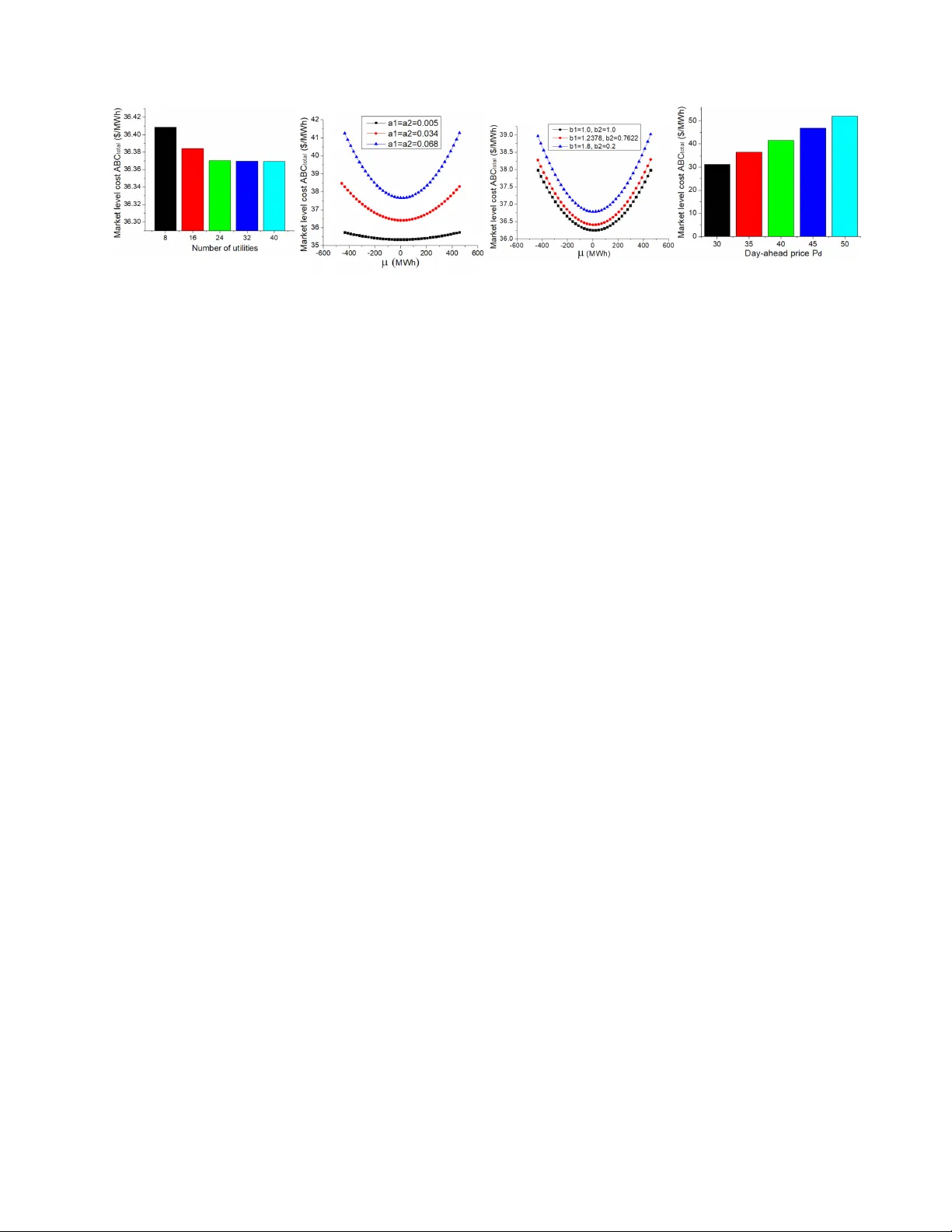
1 Ef ficient and Rob ust Equilibrium Strategies of Utilities in Day-ahead Market with Load Uncertainty T ianyu Zhao, Hanling Y i, Minghua Chen, Chenye W u, and Y unjian Xu Abstract W e consider the scenario where N utilities strategically bid for electricity in the day-ahead market and balance the mismatch between the committed supply and actual demand in the real-time market, with uncertainty in demand and local renewable generation in consideration. W e model the interactions among utilities as a non-cooperative game, in which each utility aims at minimizing its per-unit electricity cost. W e inv estigate utilities’ optimal bidding strategies and show that all utilities bidding according to (net load) prediction is a unique pure strategy Nash Equilibrium with two salient properties. First, it incurs no loss of efficiency; hence, competition among utilities does not increase the social cost. Second, it is robust and (0, N − 1 ) fault immune. That is, fault beha viors of irrational utilities only help to reduce other rational utilities’ costs. The expected market supply-demand mismatch is minimized simultaneously , which improv es the planning and supply-and-demand matching efficienc y of the electricity supply chain. W e prove the results hold under the settings of correlated prediction errors and a general class of real-time spot pricing models, which capture the relationship between the spot price, the day-ahead clearing price, and the market-le vel mismatch. Simulations based on real-world traces corroborate our theoretical findings. Our study adds new insights to market mechanism design. In particular , we deriv e a set of fairly general sufficient conditions for the market operator to design real-time pricing schemes so that the interactions among utilities admit the desired equilibrium. Index terms— Electricity Market, Bidding Strategy , Nash Equilibrium, Electricity Price, Fault Immunity , Load Uncertainty , Distributed Renew able Generation. I . I N T RO D U C T I O N Modern power system has been actively practicing deregulated electricity supply chain since the reform in 1990’ s [1]. As illustrated in Fig. 1, the deregulated supply chain usually consists of generation companies, utility companies, and sectors in char ge of transmission and distrib ution networks [2]. In particular , utilities obtain power supply from the regional electricity market and local renewable sources to serve households and microgrids. The market operator (known as independent system operator (ISO), e.g., ISO New England (ISO-NE) [3]) provides a trading place and matches the supply offers and demand bids at two different timescales and prices [4]–[6]. T ianyu Zhao and Hanling Y i are with Information Engineering, The Chinese Univ ersity of Hong Kong. Minghua Chen is with School of Data Science, City University of Hong K ong. Chenye W u is with School of Science and Engineering, The Chinese University of Hong Kong, Shenzhen. Y unjian Xu is with Mechanical and Automation Engineering, The Chinese Univ ersity of Hong Kong. 2 Fig. 1. The deregulated electricity supply chain. • Day-Ahead Market: Generation companies (utilities) submit offers (bids) for selling (buying) electricity one day before the actual dispatch, based on generation (net load) forecasting. They are cleared at a market clearing price. • Real-T ime Market: Real-time market is designed to resolve the imbalance between the actual real-time demand and the committed supply purchased from the day-ahead market, on an hourly basis. W e remark that the real- time electricity price depends on both the day-ahead clearing price as well as the real-time market lev el imbalance. New Y ork Independent System Operator (NYISO) reports that while roughly 95% of the electricity load is scheduled in the day-ahead market transaction, 5% of that remains to be settled in the real-time market [7]. The cost of the utility is composed of the payment in the day-ahead market and the expense in the real-time market to resolve the imbalance. 1 Although the existing electricity market is not a free mark et and is regulated to a certain degree, utilities can still play strategically to lo wer their own costs. In particular , in the day-ahead market, utilities can overb uy (respecti vely underbuy) electricity giv en the load forecasting results, expecting they can sell the surplus in the real-time market at a higher price (respectively buy the shortage at a lo wer price). W e remark that utilities interact with each other in this process. The cost of a utility depends on both its o wn bidding strategy and those of all other utilities since the latter affect the real-time market-le vel imbalance and consequently the real-time spot price. A. Related W ork There hav e been a number of works studying the optimal bidding strategies of generation companies in order to minimize their operating costs on the supply side of the electricity supply chain [14]–[30]; see e.g., [19] for a survey . In particular, generation companies deri ve their optimal decisions by solving the scheduling problems that seek optimal production schedules. For example, study [15] proposes an equilibrium problem with equilibrium 1 Similar to [8]–[13], we do not consider the intra-day market as its trading quantity is negligible as compared to the day-ahead and real-time markets. 3 constraints (EPEC) framework to analyze the strategic beha viors of electricity producers owning dispatchable wind power units. Study [16] formulates the Cournot competition model to analyze the interactions among generation firms with production uncertainty . The impact of coalition on the game equilibrium is explored. As the intermediary between consumers and the dere gulated electricity market, utilities’ optimal bidding strate gies and their interactions hav e also been activ ely in vestigated in many studies on the demand side of the electricity market, mainly on two aspects. The first is on the optimal bidding strategies of utilities. This includes characterizing the maximum profit for individual utility in the market [31], [32] and designing optimal bidding decisions [33]–[35]. W e note that the e xisting works mainly focus on formulating the demand side optimization problems to obtain utilities’ optimal decisions under various scenarios, e.g., time-series methods, data-driv en predictions, and genetic algorithms are discussed in [8], [36]. Howe ver , the analysis on the market equilibrium structure and properties may not be included, especially considering demand uncertainty in the two-settlement electricity market. The first cate gory is in vestigating the optimization methods and frameworks considering demand response [9], [12], [37]–[42]. F or example, a short-term planning model to determine the bidding strategies for utilities with flexible po wer demand is proposed in [9]. The second cate gory is applying stochastic programming models to incorporate price and demand uncertainties [43]–[47]. This includes deriving utilities’ optimal strategies and the market clearing mechanism under various probabilistic scenarios. For example, study [46] presents a multistage stochastic demand-side management model to solves a large-scale extended time-horizon strategic electricity consumption scheduling problem. The impact of the strategic behavior of a major consumer with flexible load is shown. A stochastic market clearing mechanism that considers deviation costs and demand uncertainty is introduced in [45]. The thir d category focuses on the market equilibrium characterization [35], [45], [48]–[50], which in volv es utilities’ interactions, e.g., the authors in [49] employ the EPEC optimization model to represent the interaction between the market participants. The sufficient conditions for the existence of such equilibrium are established. Study [35] formulates the day-ahead grid optimization as a generalized Nash equilibrium problem (GNEP). Conditions for the existence of GENP solutions and the conv erging algorithm are proposed. Besides focusing on attaining the market equilibrium, the authors in [51] propose a coevolutionary approach to in vestigate indi vidual and cooperative strate gies of utilities in a power market. The impact of cooperative behavior by forming coalitions is shown. In addition to the three categories described above, there has been a line of research on studying utilities’ behaviors [52], [53] and market efficiency [54] under some specific scenarios. Study [52] proposes a scheduling model for utilities’ energy storage operation with CV aR as a risk metric to cope with price and load uncertainties. [54] characterizes a real-time retail pricing model to in vestigate the competitiv e electricity market stability and efficienc y . The interactions between utilities, consumers, and wholesale electricity market are studied in [53]. Due to the uncertain demand and the fast penetration of intermittent renewables, there is a series of studies further study the impact of load uncertainty , i.e., how renewables and demand uncertainty w ould affect utilities’ net load predictions [55] and costs [56], besides containing such modeled uncertainty [31] in the optimization programs discussed above. It is observed that renewable penetration is likely to deteriorate load prediction errors [56], and consequently , net load uncertainty will affect utilities’ costs [55]–[60]. For instance, in our previous work [55], H. 4 Y i et al. show that larger renewable penetration degrades prediction accuracy , leading to higher load uncertainty . The corresponding local impact and global impact of such uncertainty are in vestig ated. It is demonstrated that load uncertainty can cause an increase in utilities’ costs It should be noted that electricity price forecasting is also fundamental for energy companies’ decision-making mechanisms [61], [62]. Utilities inv olved in the electricity market are faced with the uncertainty challenge of volatile power market prices in their daily operations, and prior knowledge of such price fluctuations can help them set up corresponding bidding strate gies so as to maximize their profit [63]. Hourly ener gy price is a comple x signal due to its nonlinearity , nonstationarity , and time-variant behavior [64], [65]. Multiple probabilistic price forecasting models and frameworks are proposed to approximate the parameters of the probability density function for the hourly price variables based on past prices, po wer loads, chronological information, etc [66]–[68]. Our work differs from the existing literature in that, we consider the demand side bidding under the game- theoretical setting with load uncertainty in the two-settlement electricity market and we in vestigate the uniqueness and efficienc y of the market equilibrium according to its structure. Equilibrium robustness and the aggre gate impact of all utilities’ bidding strategies on the individual utility’ s cost are also studied. The explicit form of utilities’ optimal bidding strategies and the market equilibrium can be deriv ed. Furthermore, besides designing the optimal decisions of utilities, our study adds new insights to mark et mechanism design and market operation. In particular , we sho w that if the market operator can design the real-time pricing scheme to meet a set of fairly general sufficient conditions described in Sec. IV, then the utility bidding game will admit a unique pure Nash Equilibrium without loss of efficienc y , and it is robust to irrational utilities’ fault behaviors. Meanwhile, the expected total market supply-demand mismatch can be minimized simultaneously , which improv es the planning and supply-and-demand matching efficiency of the electricity supply chain. B. Contributions W e formulate the interactions among utilities as a non-cooperativ e game. Utilities aim at minimizing individual costs by optimizing their own bidding strategies, taking into account uncertainty in load and local renew able generation. W e seek answers to three critical questions: • What is the outcome of such a utility bidding game? In particular , does there exist a pure strategy Nash Equilibrium 2 ? If so, is it unique? • Does competition introduce efficiency loss compared with the social optimal under the coordinated setting? That is, what is the loss of efficiency 3 at the equilibrium? • How robust is the equilibrium against irrational fault behaviors 4 ? In particular, will rational utilities suffer in a fault-ridden setting with irrational utilities? 2 A pure strategy corresponds to the common practice that individual utility places one bidding curve (quantity) for each trading hour in day-ahead market. 3 The ratio between the social cost at the equilibrium and the social optimal quantifies the loss of efficiency due to competition [69]. 4 An equilibrium is (  , K ) fault immune if non-fault utilities’ expected costs increase by at most  when up to K other utilities deviate arbitrarily [70]. 5 Answers to these questions provide ne w understandings of the effecti veness of the electricity market design, as well as the impact of load uncertainty . W e conduct a comprehensive study and make the following contributions. T o better bring out the insights and intuitions, we first focus on a baseline setting where the load prediction errors across utilities are mutually independent and the spot pricing model, describing the relationship among the spot price, day-ahead clearing price, and real-time market-lev el mismatch, is a class of piece-wise linear functions similar to the ones in [71], [72]. • W e show that all utilities bidding according to (net load) prediction is a unique pure strategy Nash Equilibrium. • W e show that the Nash Equilibrium incurs no loss of efficiency , i.e., the social cost of the equilibrium is the same as the optimal one under the coordinated setting. Furthermore, the equilibrium is robust and (0, N − 1 ) fault immune. That is, irrational fault behaviors of any subset of the utilities only help reduce the costs of the remaining rational utilities [70]. W e then generalize the results to the setting with correlated prediction errors and general pricing models. • W e present a set of sufficient conditions on the spot pricing model for observing the unique, efficient, and (0, N − 1 ) fault immune rob ust pure strate gy Nash Equilibrium. In particular , we sho w that our abov e results hold for correlated prediction errors and a general class of real-time spot pricing models which can be nonlinear . In Sec. V, we conduct extensiv e simulations based on price and load data from the ISO-NE electricity market. The results corroborate our theoretical findings and highlight that it is possible to design ef fective real-time pricing schemes satisfying the sufficient conditions deriv ed in our paper, such that the interactions among utilities admit a unique, efficient, and robust pure strategy Nash Equilibrium. The structure of this paper is as follows. W e first introduce the utility bidding game formulation in Sec. II. Based on the proposed game-theoretical model, Sec. III in vestigates the desired properties of the equilibrium. Sec. IV provides the generalized conditions to still admit the preferred equilibrium. Experimental results are included in Sec. V. Sec. VI deliv ers the concluding remarks. Due to the space limitation, all proofs and the summary of theoretical results are presented in the appendix. I I . P RO B L E M F O R M U L A T I O N W e consider the scenario where N utilities strategically bid for electricity in the day-ahead market and balance the mismatch between the committed supply and actual demand in the real-time market, with uncertainty in demand and local renewable generation in consideration. Since the transactions are settled on an hourly basis, we focus on a particular hour without loss of generality . W e use p d and p s (unit: $/MWh) to denote the corresponding day-ahead price and the spot price, respectively . Similar to [8], [10]–[13], [43], we consider the setting where a single utility does not ha ve market power to manipulate the day-ahead clearing prices, i.e., utilities are considered as price-takers in the day-ahead market. This setting is consistent with the situation in many liberalized electricity markets where the trading volume of most utilities is too small to influence the price as compared to the total market turno ver [9], [10], [73]. W e also consider that utilities’ bidding strategies can af fect the real-time market spot price, i.e., utilities are viewed as price-makers in the real-time market. This is reasonable as utilities’ strategic bidding behaviors can hav e significant impact in real-time balancing markets where only a small amount of energy is traded [8], [74]. 6 In practice, at the time of day-ahead bidding, utilities usually do not know precisely its load and local renewable generation. Instead, they hav e distributional information of the net load by load forecasting. For ease of analysis, we first focus on the setting that utilities only place one quantity bid for each trading hour in the day-ahead market. Our results can be generalized to the case in which utilities submit demand curves as bidding pairs (price, quantity); see Sec. IV -C for a discussion. A. Utility bidding and Load Mismatch Modeling W e define D i (unit: MWh) as utility i 0 s actual net load at a particular hour , and it is only re vealed to the utility in the real-time manner . When utility i participates in day-ahead market, it has a prediction of D i , denoted as ˆ D i , modeled as follows: ˆ D i = D i +  i , (1) where  i is a random v ariable representing the load prediction error . It is af fected by the uncertainties of demand and local renew able generation o wned by the utilities and microgrids. Giv en the load prediction ˆ D i , utility i can strategically participate in the day-ahead market by bidding a quantity Q i , ˆ D i − µ i , where • µ i = 0 : Utility bids precisely according to prediction. • µ i > 0 : Utility strategically underbuys. • µ i < 0 : Utility strategically overb uys. W e use µ i to represent the bidding strategy of utility i . The bidding strategy of utility i will affect its mismatch between the real-time actual net load and the day-ahead purchased supply in the real-time market, which is denoted as ∆ i (unit: MWh). By definition, we have ∆ i , D i − Q i = µ i −  i . (2) Whenev er there is an imbalance, i.e., ∆ i 6 = 0 , the utility has to settle this imbalance in the real-time market at the spot price p s . It either sells the residual electricity back to the market when ∆ i < 0 , or buys the deficient electricity from the market when ∆ i > 0 . For ease of presentation, we define ∆ , N X i =1 ∆ i , and ∆ − i , N X j : j 6 = i ∆ j (3) as the market-le vel mismatch and the aggregate mismatch of all other utilities except utility i , respectiv ely . B. Real-time Market Spot Pricing Model The real-time mark et price generally depends on the market-le vel supply and demand imbalance, i.e., the dif ference between the day-ahead scheduled supply and the real-time actual demand. Deficient supply in the market leads to 7 a higher spot price (up-regulation), whereas excessi ve supply results in a lower spot price (down-re gulation). T o capture their relationship, we consider the following piece-wise linear pricing model 5 [72]; see Fig. 2 for illustration. p s =            p d , ∆ = 0; ( a 1 ∆ + b 1 ) p d , ∆ > 0; ( a 2 ∆ + b 2 ) p d , ∆ < 0 . (4) Here a 1 , a 2 , b 1 , b 2 ∈ R + are parameters of the pricing model. Fig. 2. Real-time piece-wise linear pricing model of p d and total imbalance ∆ . Remark: (i) The model was proposed in [72] by curve-fitting the historical data. In general, a 1 6 = a 2 , b 1 6 = b 2 . Specifically , [72] suggests a 1 = 0 . 0034 , a 2 = 0 . 0005 , b 1 = 1 . 2378 , and b 2 = 0 . 6638 . (ii) The spot price function is discontinuous at ∆ = 0 , i.e., b 1 > 1 > b 2 . This discontinuity models the pr emium of readiness that utilities need to pay for the generation companies, since they hav e to generate urgent regulating power [71]. (iii) In this paper, we first focus on the piece-wise linear symmetric pricing model, i.e., a 1 = a 2 > 0 , ( b 1 p d + b 2 p d ) / 2 = p d , and b 1 > b 2 . Then in Sec. IV, we generalize our results to a larger class of pricing models, which can be nonlinear or continuous at the origin. C. Cost Function of Utilities and Strate gic Bidding Game For utility i , its electricity procurement is settled in two timescales: (i) an amount of D i − ∆ i is settled in the day-ahead market at price p d , and (ii) the remaining amount ∆ i is settled in the real-time market at the spot price p s . Hence the total electricity cost of utility i is giv en as follo ws (unit: $): ˜ C i = p d  ˆ D i − µ i  + p s ∆ i = p d ( D i − ∆ i ) + p s ∆ i . (5) 5 Generation imbalance from generation companies’ side also proposes an effect on the real-time market electricity price, e.g., in case of generator failure or the uncertainty from large-scale renewable generation. Such imbalance may increase the market mismatch variability . This paper mainly focuses on the demand side of the electricity market, and the effect of generation uncertainty on the market imbalance is not considered. W e leave the incorporation of generation uncertainty into market equilibrium analysis for future study . 8 The A verage Buying Cost per unit electricity ( ABC ) for utility i is simply ABC i , ˜ C i D i = 1 D i [ p d ( D i − ∆ i ) + p s ∆ i ] . (6) Consider the net load uncertainty , the cost function for utility i is defined as the expected ABC i , i.e., C i ( µ i , µ − i ) , E [ ABC i ] . (7) Note that the cost of utility i not only depends on its own strategy µ i but also depends on µ − i , P N j : j 6 = i µ j , the aggregate strategies of all other utilities. The underlying reason is that the real-time spot price is determined by the market-le vel mismatch, and other utilities’ strategic beha vior can af fect the cost of utility i through the spot price p s . Giv en the model of strategic behaviors and utilities’ cost functions, we model their interactions as a non- cooperativ e game with N utilities where each utility aims to minimize its own cost C i ( µ i , µ − i ) by choosing a strategy represented by µ i . Formally , a strategy profile µ ∗ = ( µ ∗ 1 , µ ∗ 2 , ..., µ ∗ N ) constitutes a Nash Equilibrium if for each i = 1 , 2 , ..., N , C i ( µ ∗ i , µ ∗ − i ) ≤ C i ( µ i , µ ∗ − i ) , ∀ µ i ∈ R , (8) where R is the set of real numbers. I I I . M A I N R E S U LT S : M A R K E T E Q U I L I B RI U M A NA LY S I S Under the two-settlement market mechanism, we study the Existence , Uniqueness , Efficiency , and Rob ustness of the equilibrium of the game among utilities. In this section, we consider the scenario that the net load prediction errors  1 , ...,  N are mutually independent and the real-time spot pricing model is piece-wise linear symmetric as defined in (4) with a 1 = a 2 , ( b 1 p d + b 2 p d ) / 2 = p d , and b 1 > b 2 . These two settings allow us to better highlight the impacts of utilities’ strategies and the market equilibrium characteristics. W e later extend the results to the case with correlated prediction errors and general pricing models in Sec. IV. A. Load Imbalance Distribution and Analysis of Utilities’ Strate gic Behaviors W e model the net load prediction error  i as a general symmetric unimodal random v ariable with zero mean and variance σ 2 i . Definition 1. A pr obability density function f X ( · ) is symmetric unimodal if it is (i) Symmetric w .r .t. its mean ξ : f X ( ξ + x ) = f X ( ξ − x ) , ∀ x ∈ R ; (9) (ii) Central dominant: f X ( x ) ≤ f X ( y ) , if | x − ξ | ≥ | y − ξ | , ∀ x, y ∈ R . (10) 9 Her e ξ , R + ∞ −∞ x · f X ( x ) dx is the expected value of X . Many prediction error distributions are symmetric unimodal, including Gaussian distribution and Laplace distri- bution. W e say that a random v ariable is symmetric unimodal if it follo ws a symmetric unimodal distribution. The specific meaning of central dominant comes from that utilities tend to make larger prediction errors with smaller probability compared with the case of smaller errors with larger probability . Symmetric distribution implies that utilities have equal chances to encounter positiv e or negativ e prediction errors; see Sec. V -B for details. Fig. 3. Load prediction error histogram from case study based on real-world data. Giv en a utility’ s bidding strategy µ i , the real-time imbalance ∆ i follows a symmetric unimodal distribution with mean µ i and variance σ 2 i , ∆ i ∼ P i ( µ i , σ 2 i ) , i = 1 , 2 , ..., N . (11) Lemma 1. The sum of independent symmetric unimodal random variables is still symmetric unimodal. That is, suppose that ther e are N independent random variables ∆ 1 , ..., ∆ N , and for each i = 1 , 2 , ..., N , ∆ i follows a symmetric unimodal distribution with mean µ i , then their sum ∆ , P N i =1 ∆ i follows a symmetric unimodal distribution with mean µ = P N i =1 µ i . In addition, if ther e exists one ∆ i whose pr obability density function is strictly central dominant, i.e., f ∆ i ( x ) < f ∆ i ( y ) , if | x − ξ | > | y − ξ | , ∀ x, y ∈ R , (12) then the pr obability density function of ∆ is also strictly central dominant. Lemma 1 states the property of the con volutions of symmetric unimodal random v ariables [75]. W e present here a stronger observation on such distribution con volutions. Applying Lemma 1, we have ∆ ∼ P ( µ, σ 2 ) , and ∆ − i ∼ P − i ( µ − i , σ 2 − i ) , (13) 10 where µ , P N i =1 µ i , µ − i , P N j : j 6 = i µ j , σ 2 , P N i =1 σ 2 i , and σ 2 − i , P N j : j 6 = i σ 2 j . Based on the abov e observ ations, Theorem 1 characterizes the cost function C i ( µ i , µ − i ) = E [ ABC i ] of utility i . Theorem 1. Under independent pr ediction error s and piece-wise linear symmetric spot pricing model, the expec- tation of ABC i is given as: E [ ABC i ] = p d + p d D i  a 1 + a 2 2 ( µ i µ − i + σ 2 i + µ 2 i ) +( b 1 − b 2 ) E h ∆ i · ˜ F (∆ i ) ii , (14) wher e ˜ F (∆ i ) , R µ − i − ∆ i f ∆ − i ( δ − i ) dδ − i , f ∆ − i ( · ) is the PDF of ∆ − i with mean µ − i , and coefficients a 1 , a 2 , b 1 , b 2 ar e parameters of the spot pricing model defined in (4). Remarks: Utility estimates its expected cost via (14) considering load uncertainty . The expectation of ABC i in (14) depends on three terms. The first term is simply the day-ahead market clearing price. The second and the third terms represent the real-time mark et operation cost to balance the mismatch. It is clear that the strategic behavior of utility i and the aggregation of all other utilities’ strategies affect both the second and the third terms. In addition, the second term re veals the influence of the pricing model slope, and the third term presents the discontinuous part of the pricing model. Meanwhile, given µ − i = 0 , both term two and term three are positive and E [ ABC i ] will increase under the following conditions. • The day-ahead market clearing price p d increases. • The slope of the real-time market pricing model increases, i.e., a 1 , a 2 increases, • The discontinuity gap of the pricing model b 1 − b 2 increases. In Sec. V -D, our simulation results verify these observations. The results show that utilities suffer higher costs under higher day-ahead clearing price and larger real-time market sensitivity . Note that in day-ahead market operations, the actual net load D i is not realized precisely to utilities, and they only estimate their expected cost via (14). Our following results show that utilities’ optimal bidding strategy is independent of the specific value of D i . Therefore, utilities can still deriv e their optimal operations ev en in absence of the full knowledge of D i ; accordingly , the market equilibrium can be described. B. Existence and Uniqueness of the Nash Equilibrium A Nash Equilibrium in the utility bidding game is a strategic profile in which all utilities choose the optimal strategy that minimizes its own cost given others’ behaviors. W e start by understanding the characteristics of the third term in (14). Lemma 2. Given µ − i = 0 , the optimal µ ∗ i that minimizes E h ∆ i · ˜ F (∆ i ) i is 0, and it is strictly incr easing w .r .t. | µ i | , the absolute value of µ i . Lemma 2 shows that the third term in (14) that related to the discontinuous part of the spot pricing model will increase if the utility deviates from bidding according to prediction, gi ven that the aggregation of all other utilities’ strategies is zero. 11 Recall that utilities only place one quantity for one bid in the market; it is sufficient to focus on the pure strate gy Nash Equilibrium. W ith Theorem 1 and Lemma 2, we present the following necessary condition for all pure strategy Nash Equilibria. Theorem 2. Under independent pr ediction err ors and piece-wise linear symmetric spot pricing model, a strate gy pr ofile µ ∗ = ( µ ∗ 1 , µ ∗ 2 , ..., µ ∗ N ) constitutes a pure strate gy Nash Equilibrium only if for all i = 1 , 2 , ..., N , • µ ∗ i = 0 , if µ ∗ − i = 0; • µ ∗ i ∈  − µ ∗ − i , 0  , if µ ∗ − i > 0; • µ ∗ i ∈  0 , − µ ∗ − i  , if µ ∗ − i < 0 . (15) Remarks: Theorem 2 sho ws the structure of utilities’ optimal bidding strate gies. It says that if µ − i = 0 , then the best response of utility i is to choose µ ∗ i = 0 . If µ − i 6 = 0 , then utility i 0 s optimal strategy will always be opposite to this value. The insights behind Theorem 2 and utilities’ optimal bidding strategies at equilibrium can be revealed from the perspectiv e of cost minimization and best response. W e note that when the utility’ s real-time mismatch has the same sign as the market-le vel mismatch, the utility will suffer a loss; otherwise, it will gain. For example, when the market-le vel mismatch is positive, the real-time price is higher than the day-ahead price according to the pricing model. If the utility’ s mismatch is negati ve, it means that the utility b uys e xcessi ve energy in the day-ahead market and it can sell it back to the market at a higher price. Thus the utility will gain. W ith this in mind, let us look at the case when utility i chooses the bidding strategy µ i > 0 , given µ − i = 0 . Recall that the utility’ s prediction error follo ws a symmetric unimodal distrib ution with mean zero, which indicates it has the same possibility to encounter particular positiv e or negati ve errors. Consequently , if the utility strategically underbuys when participating in the day-ahead mark et, i.e., µ i > 0 , its real-time imbalance will tend to be negativ e. Since the market-lev el mismatch follows a symmetric unimodal distribution P ( µ i , σ 2 ) , when µ i > 0 , the market- lev el mismatch and the utility i 0 s mismatch tend to be positiv e simultaneously , thus the utility i tends to suffer a loss. Similarly , when µ i < 0 , giv en µ − i = 0 , the utility i will also suffer a loss. Then we consider the cases when µ − i 6 = 0 . If µ − i > 0 , the utility i will not choose µ i > 0 since this will make the market imbalance hav e more tendency to be positive. A similar result holds for the case when µ i < − µ − i . These two situations expose the utility to the risk that its imbalance has more possibility to hav e the same sign with the mark et-le vel imbalance. Furthermore, choosing µ i to be less than 0 and greater than − µ − i will alw ays be better than µ i = 0 and µ i = − µ − i . The optimal µ ∗ i comes from the trade-off between the price and the amount. Similarly , when µ − i < 0 , utility i will choose µ i ∈ (0 , − µ − i ) . Suppose ( µ ∗ 1 , µ ∗ 2 , ..., µ ∗ N ) is a pure strategy Nash Equilibrium profile with m non-zero elements, where 1 ≤ m ≤ N . According to Theorem 2, for these m elements, denoted as ( µ ∗ 1 , µ ∗ 2 , ..., µ ∗ m ) without loss of generality , we define α i , µ ∗ i µ ∗ − i ∈ ( − 1 , 0) , ∀ i ∈ { 1 , 2 , ..., m } . (16) 12 It is straightforward to derive the following condition:         − 1 α 1 . . . α 1 α 2 − 1 . . . α 2 . . . . . . . . . . . . α m α m . . . − 1                 µ ∗ 1 . . . . . . µ ∗ m         =         0 . . . . . . 0         , (17) which describes the second and the third conditions in (15) for all non-zero µ i . Let M be the left-hand side m × m matrix. W e have the following results. Theorem 3. Under independent prediction err ors and piece-wise linear symmetric spot pricing model, the matrix M is a full rank matrix, and consequently µ ∗ = 0 is the unique pur e strate gy Nash Equilibrium. Theorem 2 and Theorem 3 imply that for any day-ahead clearing price p d , 6 if all utilities except utility i bid according to prediction, then bidding according to prediction is the best response of utility i (see Fig. 7 based on real-world data for illustration). Consequently , all utilities bid exactly according to (net load) prediction is the unique pure strategy Nash Equilibrium. Conv entionally , Nash Equilibrium indicates that a utility does not benefit from deviating from the equilibrium, assuming other utilities keep their strategies unchanged. In Corollary 1, we show a stronger characteristic of the equilibrium. That is, the cost of the utility is strictly increasing w .r .t. the deviation distance between the strategy chosen and the equilibrium. Corollary 1. Under independent prediction err ors and piece-wise linear symmetric spot pricing model, given µ − i = 0 , the optimal µ ∗ i that minimizes E [ ABC i ] is 0, and E [ ABC i ] is strictly increasing w .r .t. | µ i | . In Sec. IV, we generalize the results to the case of correlated prediction errors (across utilities), general pricing models, and the setting in which utilities submit bidding curves considering the uncertainty of the day-ahead clearing prices. C. Efficiency and Robustness of the Nash Equilibrium W e have shown that µ ∗ = ( u ∗ 1 , u ∗ 2 , ..., u ∗ N ) = 0 is the unique pure strategy Nash Equilibrium. The next natural question is: what is the corresponding loss of efficienc y? Recall that loss of efficienc y is characterized as the gap between the social costs under the game-theoretical strate gic setting, i.e., the social cost at the equilibrium, and the coordinated setting. The optimal social cost under the coordinated setting is obtained by solving the following cost minimization problem: min µ i ∈ R , ∀ i ∈{ 1 , 2 ,...,N } E [ ABC total ] , (18) 6 The day-ahead clearing price is not known precisely to utilities beforehand. See Sec. I-A for discussions on electricity price forecasting and uncertainty . 13 where ABC total is defined as: ABC total , C total D total = P i D i · ABC i P i D i = 1 D total [ p d ( D total − ∆) + p s ∆] . (19) Here ∆ follows a symmetric unimodal distribution with mean µ = P N i =1 µ i , and ABC total (unit: $/MWh) can be interpreted as the unit cost of the market to settle D total , P N i =1 D i amount of electricity . Theorem 4. Under independent prediction err ors and piece-wise linear symmetric spot pricing model, E [ ABC total ] is minimized at µ ∗ = 0 , and E [ ABC total ] is strictly increasing w .r .t. | µ | . Consequently , the unique pure strate gy Nash Equilibrium µ ∗ = 0 incurs no loss of efficiency . Remarks: Theorem 4 shows the market operator that the social cost at the equilibrium is the same as the optimal one under the coordinated setting in (18). The intuition behind Theorem 4 lies in that we can treat the whole market as an entity . From the market-lev el perspectiv e, an amount of ( D total − ∆) power is committed at the price p d and the imbalance ∆ is settled at the spot mark et price p s . When the market has a particular positive (respecti vely negati ve) real-time mismatch, this mismatch is settled at a price p s > p d (respectiv ely p s < p d ); hence the market will suffer a loss. Since the market mismatch ∆ follo ws a symmetric unimodal distribution P ( µ, σ 2 ) , when µ > 0 , the market-lev el mismatch tends to be positiv e, thus the market tends to suffer a loss facing a higher spot price. Similar analysis can be applied to the case when µ < 0 . W e conclude that the unique pure strategy Nash Equilibrium is efficient; see Fig. 7 for illustration. The guarantee provided by a Nash equilibrium is that each player’ s strate gy is optimal, assuming all others play their designated strategies. Howe ver , there could exist fault behaviors, wherein some utilities are irrational, and their actions can be arbitrary or even adversarial. In the following theorem, we illustrate a strong observation on the robustness of the equilibrium. That is, the sub-optimal response faults behaviors of irrational utilities not only increase their own costs but also benefit other rational utilities. Theorem 5. Under independent pr ediction err ors and piece-wise linear symmetric spot pricing model, the equilib- rium µ ∗ = 0 is (0, N − 1 ) fault immune. That is, consider all utilities except a gr oup of utilities S , S ⊂ { 1 , 2 , ..., N } and 1 ≤ | S | ≤ N − 1 . Given µ j = 0 , ∀ j ∈ { 1 , 2 , ..., N }\{ S } , E [ ABC j ] is non-increasing w .r .t. | µ S | , where µ S = P i ∈ S µ i . In addition, if there exists one  k , k ∈ { 1 , 2 , ..., N } , whose probability density function is strictly central dominant, 7 then E [ ABC j ] is strictly decreasing w .r .t. | µ S | . Theorem 5 sho ws the robustness of the unique pure strate gy Nash Equilibrium µ ∗ = 0 . This is a desirable property as discussed in [70]. It provides the utility an understanding of its cost change characteristic w .r .t. irrational market participants’ actions. The result indicates that fault behaviors of irrational utilities will not increase the costs of other rational utilities; see Fig. 4 for illustration. 7 see Lemma 1 for the definition of strictly central dominant. 14 Fig. 4. Illustration of the (0, N − 1 ) fault immune robustness of the pure strategy Nash equilibrium under piece-wise linear symmetric pricing model and Gaussian distributed prediction errors. I V . M A I N R E S U L T S : E QU I L I B R I U M G E N E R A L I Z A T I O N Previous analysis focuses on the scenario where the real-time market pricing model is piece-wise linear symmetric and prediction errors of utilities are mutually independent and utilities only place one quantity bid in the day ahead market. In this section, we extend our results to the setting with correlated prediction errors, general pricing models, and utilities submitting bidding curves as bidding pairs ((price, quantity) considering the uncertain day-ahead prices. A. Be yond Piece-W ise Linear Symmetric Spot Pricing Model The uniqueness, ef ficiency , and rob ustness of the pure strategy Nash Equilibrium hold for a large class of pricing models which can be nonlinear or continuous at the origin. Theorem 6. Suppose the net load prediction err ors are mutually independent. Denote the pricing model as: p s =            p d , ∆ = 0; p (∆) + b 1 p d , ∆ > 0; p (∆) + b 2 p d , ∆ < 0 . (20) Her e b 1 + b 2 = 2 , b 1 ≥ b 2 , p (∆) is a non-decreasing odd function, i.e., p (∆) = − p ( − ∆) and p ( x ) ≥ p ( y ) , ∀ x ≥ y , and p (∆) is continuous at ∆ = 0 . The following statements are true: (1) Given µ − i = 0 , the optimal µ ∗ i that minimizes E [ ABC i ] is 0, and E [ ABC i ] is non-decr easing w .r .t. | µ i | . Consequently , µ ∗ = ( µ ∗ 1 , µ ∗ 2 , ..., µ ∗ N ) = 0 is a pure strate gy Nash Equilibrium. In addition, if p (∆) is strictly incr easing w .r .t. ∆ or b 1 > b 2 , then E [ ABC i ] is strictly increasing w .r .t. | µ i | . (2) If p ( · ) is differ entiable for all x ∈ R , and p 0 ( x 1 ) ≥ p 0 ( x 2 ) > 0 , ∀ x 1 > x 2 ≥ 0 , p 0 ( x 1 ) ≥ p 0 ( x 2 ) > 0 , ∀ x 1 < x 2 ≤ 0 , (21) then µ ∗ = 0 is the unique pur e strate gy Nash Equilibrium. 15 (3) E [ ABC total ] is minimized at µ ∗ = 0 , and E [ ABC total ] is non-incr easing w .r .t. | µ | . Consequently , the pure strate gy Nash Equilibrium µ ∗ = 0 incurs no loss of efficiency . In addition, if p (∆) is strictly incr easing w .r .t. ∆ or b 1 > b 2 , then E [ ABC total ] is strictly increasing w .r .t. | µ | . (4) If p ( · ) is differ entiable for all x ∈ R , and either b 1 > b 2 , p 0 ( x 2 ) ≥ p 0 ( x 1 ) ≥ 0 , ∀ x 1 > x 2 ≥ 0 , p 0 ( x 2 ) ≥ p 0 ( x 1 ) ≥ 0 , ∀ x 1 < x 2 ≤ 0 , (22) or p 0 ( x 2 ) > p 0 ( x 1 ) ≥ 0 , ∀ x 1 > x 2 ≥ 0 , p 0 ( x 2 ) > p 0 ( x 1 ) ≥ 0 , ∀ x 1 < x 2 ≤ 0 , (23) then the pur e strate gy Nash Equilibrium µ ∗ = 0 is (0, N − 1 ) fault immune. Remarks: (i) The general pricing models defined in (20) are described by the discontinuous gap ( b 1 − b 2 ) · p d and the imbalance related term p (∆) . The results in Sec. III are for the special case of Theorem 6 of the piece-wise linear symmetric pricing model. (ii) Theorem 6 indicates that the results of the uniqueness, efficiency , and (0, N − 1 ) fault immune robustness of the equilibrium obtained in Sec. III can be extended to the case with general pricing models, which can be nonlinear or continuous at the origin. (iii) Pricing models satisfying (21) are con ve x when ∆ > 0 and concave when ∆ < 0 . The pricing models satisfying (22) or (23) are concav e when ∆ > 0 and con vex when ∆ < 0 ; see Fig. 5 for illustration. Therefore, the piece-wise linear symmetric pricing model with discontinuous gap at the origin is the only one that satisfies both (21) and (22) or (23) and thus admits the unique, efficient, and (0, N − 1 ) fault immune robust pure strategy Nash Equilibrium. (a) Discontinuous symmetric pricing model: b 1 = 1 . 2378 , b 2 = 0 . 7622 . (b) Continuous symmetric pricing model: b 1 = b 2 = 1 . Fig. 5. Nonlinear pricing function p ( x ) = p d × (1 { x> 0 } ( a 1 x k + b 1 ) + 1 { x< 0 } ( − a 2 ( − x ) k + b 2 ) + 1 { x =0 } ) with a 1 = a 2 = 0 . 0034 , p d = 35 , k = 1 . 15 satisfying (21) and k = 0 . 9 satisfying (23), where 1 {·} is the indicator function. T o show the nonlinear relationship more clearly and let the price within the reasonable range, we vary ∆ from -0.1GWh to 0.1GW . 16 B. Be yond Independent Pr ediction Err ors In practice, load prediction errors among utilities may be correlated; see e.g., [76]. In this subsection, we generalize our results and consider the case that utilities’ prediction errors  i follow correlated Gaussian distributions with non-negati ve correlation coefficients ρ i,j , Cov (  i ,  j ) /σ i σ j ≥ 0 . W e obtain the following results. Theorem 7. Suppose the r eal-time spot pricing model is piece-wise linear symmetric, and  i . i = 1 , 2 , ..., N , ar e zer o mean Gaussian random variables with non-ne gative correlations, then the strate gy profile µ ∗ = 0 is the unique, efficient, and (0, N − 1 ) fault immune r obust pur e strate gy Nash Equilibrium. Practically , the load prediction errors are usually observed to be positively correlated [55], [76]. Theorem 7 highlights that with non-negativ ely correlated Gaussian prediction errors, the market still admits the equilibrium with the desired properties. C. Be yond Submitting Quantity Bid In modern deregulated electricity market, market participants are always allowed to react to the uncertain market prices since they may encounter short-term price fluctuation [9], [10], [12], [53]. Specifically , generation companies and utilities submit their selling and buying bidding curves, then the ISO compiles these submitted bidding curves and calculates the clearing price for each trading period. A certain volume of electricity is agreed for a utility according to the clearing price and its bidding curve. The bidding curve of each individual utility represents its willingness for procuring dif ferent amounts of electricity from the market under different prices. In this subsection, we extend our results to the setting in which utilities submit bidding pairs (price, quantity) which form their bidding curves for each hour considering the uncertain market clearing prices. . Similar to the previous formulation, let D i and ˆ D i be the actual net load and the net load prediction. Furthermore, we use Q i ( p d ) to denote the bidding curve of utility i , which represents the desired buying quantity under different day-ahead uncertain clearing price p d . Therefore, utility i 0 s bidding strategy and the aggregate strategies of all other utilities can be represented by µ i ( p d ) , ˆ D i − Q i ( p d ) and µ − i ( p d ) , P N j 6 = i µ j ( p d ) respectively . W e model µ i ( p d ) as piece-wise continuous functions defined on R + for each i = 1 , 2 , ..., N . Since the day-ahead clearing price p d is not known to the utilities beforehand, 8 when considering the random- ization of p d , utilities report demand bidding curves and aim at minimizing their expected costs, the probability- weighted sum of E [ ABC i | p d = ˆ p d ] , i.e., C i ( µ i ( p d ) , µ − i ( p d )) , Z + ∞ 0 E [ ABC i | p d = ˆ p d ] f i ( ˆ p d ) d ˆ p d , (24) where f i ( · ) is a piece-wise continuous probability density function defined on the set of positiv e real number R + , which represents utility i 0 s estimation on the day-ahead price p d . Here we use ( ABC i | p d = ˆ p d ) to denote utility’ s cost at day-ahead price ˆ p d . Note that we focus on the setting where utilities are price-takers in the day-ahead market and therefore their individual strategies will not affect f i ( · ) , their estimations of p d . 8 The day-ahead clearing price is not known precisely to the utilities beforehand. Utilities can have a probabilistic density forecast of electricity price by multiple probabilistic price forecasting models. W e refer to Sec. I-A for a discussion on electricity price forecasting. 17 Consequently , under the setting in which utilities submit bidding curves, a strate gy profile µ ∗ ( p d ) = ( µ ∗ 1 ( p d ) , µ ∗ 2 ( p d ) , ..., µ ∗ N ( p d )) constitutes a Nash Equilibrium if for each i = 1 , 2 , ..., N , C i ( µ ∗ i ( p d ) , µ ∗ − i ( p d )) ≤ C i ( µ i ( p d ) , µ ∗ − i ( p d )) , ∀ µ i ( p d ) ∈ F + , (25) where F + is the set of all piece-wise continuous functions defined on R + . W e further define the corresponding optimal social cost under coordinated setting, which is obtained by solving the following social cost minimization problem: min µ i ( p d ) ,i =1 , 2 ,...,N C total ( µ ( p d )) = Z + ∞ 0 E [ ABC total | p d = ˆ p d ] f ( ˆ p d ) d ˆ p d , (26) where f ( · ) is a piece-wise continuous probability density function defined on R + , which represents the ISO’ s estimation on p d . Similarly , ABC total at price ˆ p d is defined as: ( ABC total | p d = ˆ p d ) , C total D total = P i D i · ( ABC i | p d = ˆ p d ) P i D i = 1 D total [ p d ( D total − ∆( ˆ p d )) + p s ∆( ˆ p d )] . (27) Here ∆( ˆ p d ) follows a symmetric unimodal distribution with mean µ ( ˆ p d ) = P N i =1 µ i ( ˆ p d ) , and ( ABC total | p d = ˆ p d ) (unit: $/MWh) can be interpreted as the unit cost of the market to settle D total , P N i =1 D i amount of electricity at price ˆ p d . Based on the above game-theoretical formulation, we have the following results. Theorem 8. Suppose the net load pr ediction err ors are mutually independent. Denote the non-decr easing symmetric pricing model as (20) and f i ( p d ) > 0 , ∀ p d > 0 . The following statements are true: (1) Given µ − i ( p d ) = 0 , the optimal µ ∗ i ( p d ) that minimizes C i ( µ i ( p d ) , 0) is 0, and C i ( ¯ µ i ( p d ) , 0) ≥ C i ( ˆ µ i ( p d ) , 0) if | ¯ µ i ( p d ) | ≥ | ˆ µ i ( p d ) | , ∀ p d ∈ R + . Consequently , µ ∗ ( p d ) = ( µ ∗ 1 ( p d ) , µ ∗ 2 ( p d ) , ..., µ ∗ N ( p d )) = 0 is a pure strate gy Nash Equilibrium. In addition, if p (∆) is strictly increasing w .r .t. ∆ or b 1 > b 2 , then C i ( ¯ µ i ( p d ) , 0) > C i ( ˆ µ i ( p d ) , 0) if | ¯ µ i ( p d ) | ≥ | ˆ µ i ( p d ) | , ∀ p d ∈ R + and there exits an interval ( s, t ) such that | ¯ µ i ( p d ) | > | ˆ µ i ( p d ) | , ∀ p d ∈ ( s, t ) . (2) If (21) holds, µ i ( x ) is piece-wise continuous on R + , and there does not exist a point x 0 on µ i ( x ) such that µ i ( x 0 ) 6 = lim x → x − 0 µ i ( x ) and µ i ( x 0 ) 6 = lim x → x + 0 µ i ( x ) , ∀ i ∈ { 1 , 2 , ..., N } , then µ ∗ ( p d ) = 0 is the unique pur e strate gy Nash Equilibrium. (3) C total ( µ ( p d )) is minimized at µ ∗ ( p d ) = 0 , and C total ( ¯ µ ( p d )) ≥ C total ( ˆ µ ( p d )) if | ¯ µ ( p d ) | ≥ | ˆ µ ( p d ) | , ∀ p d ∈ R + . Consequently , the pur e strate gy Nash Equilibrium µ ∗ ( p d ) = 0 incurs no loss of efficiency . In addition, if p (∆) is strictly incr easing w .r .t. ∆ or b 1 > b 2 , then C total ( ¯ µ ( p d )) > C total ( ˆ µ ( p d )) if | ¯ µ ( p d ) | ≥ | ˆ µ ( p d ) | , ∀ p d ∈ R + and ther e exits an interval ( s, t ) such that | ¯ µ ( p d ) | > | ˆ µ ( p d ) | , ∀ p d ∈ ( s, t ) . (4) If (22) or (23) holds, then the pur e strate gy Nash Equilibrium µ ∗ ( p d ) = 0 is (0, N − 1 ) fault immune. 9 9 Under the setting of utilities submitting bidding curves, the corresponding (0, N − 1 ) fault immune robustness can be expressed as: consider all utilities except a group of utilities S , S ⊂ { 1 , 2 , ..., N } and 1 ≤ | S | ≤ N − 1 . Given µ j ( p d ) = 0 , ∀ j ∈ { 1 , 2 , ..., N }\{ S } , C j ( µ S ( p d ) , µ − S ( p d )) is no greater than C j ( µ ∗ S ( p d ) , µ − S ( p d )) , where µ S ( p d ) = P i ∈ S µ i ( p d ) , µ − S ( p d ) = P j ∈{ 1 , 2 ,...,N }\{ S } µ j ( p d ) = 0 , and µ ∗ S ( p d ) = 0 . In addition, if there exists one  k , k ∈ { 1 , 2 , ..., N } , whose probability density function is strictly central dominant (see Lemma 1 for definition), then C j ( ¯ µ S ( p d ) , 0) < C j ( ˆ µ S ( p d ) , 0) if | ¯ µ S ( p d ) | ≥ | ˆ µ i ( p d ) | , ∀ p d ∈ R + and there exits an interval ( s, t ) such that | ¯ µ S ( p d ) | > | ˆ µ S ( p d ) | , ∀ p d ∈ ( s, t ) . 18 Theorem 8 states that the strate gy profile that all utilities submit v ertical bidding curves 10 exactly at the predicted demand is a (0, N − 1 ) fault immune robust pure strategy Nash Equilibrium which incurs no loss of efficienc y . Furthermore, under mild continuity condition 11 on µ i ( x ) , the above ef ficient and robust equilibrium is unique; see Fig. 6(a) for illustration. (a) Bidding curve with inelastic load. (b) Bidding curve with flexible load. Fig. 6. Illustration of the pure strategy Nash Equilibrium strategies under the setting that utilities submit bidding curves at the predicted inelastic/flexible net load. W e further extend the results to the setting in which utilities submit bidding curves and their prediction errors  i follow correlated Gaussian distributions with non-negati ve correlation coefficients ρ i,j , Cov (  i ,  j ) /σ i σ j ≥ 0 . Theorem 9. Suppose the r eal-time spot pricing model is piece-wise linear symmetric, and  i . i = 1 , 2 , ..., N , ar e zer o mean Gaussian random variables with non-ne gative correlations, then the strate gy pr ofile µ ∗ ( p d ) = 0 is an efficient and (0, N − 1 ) fault immune r obust pur e strate gy Nash Equilibrium. In addition, if µ i ( x ) is piece- wise continuous on R + , and there does not exist a point x 0 on µ i ( x ) such that µ i ( x 0 ) 6 = lim x → x − 0 µ i ( x ) and µ i ( x 0 ) 6 = lim x → x + 0 µ i ( x ) , ∀ i ∈ { 1 , 2 , ..., N } , then the equilibrium is unique. Theorem 9 highlights that the equilibrium with desired properties is still admitted when utilities submit bidding curves with non-negati vely correlated Gaussian prediction errors. 10 W e focus on the setting that the net load D i is inelastic and does not change with the day-ahead clearing price p d . In reality , utilities may hav e price-related flexible demands due to dynamic pricing [9]. Therefore, the net loads D i ( p d ) may change with price p d . W e model D i ( p d ) to be piece-wise continuous for i = 1 , 2 , ..., N , and utilities’ net load prediction errors  i as symmetric unimodal random v ariables with zero mean as defined in Definition 1. Our results still hold under such setting in which utilities submit bidding curves exactly at Q i ( p d ) = ˆ D i ( p d ) that react to the market prices with flexible demands and can be generalize to the scenario with correlated prediction errors and the general pricing models; see Fig. 6(b) for illustration. 11 The continuity condition actually requires that the strategy curves µ i ( x ) do not have discontinuity points isolated from the function, which includes the continuous and piece-wise continuous bidding curves as a special case. In our model, it means that utilities will not deviate from the strategy curves at some particular points. 19 D. Impact of Load Uncertainty on Equilibrium Strate gy and Equilibrium Social Cost Note that load uncertainty is captured by the variance of the load prediction error . In this part, we discuss the impact of load uncertainty on market equilibrium strategy and social cost. Corollary 2. The utilities’ market equilibrium strate gies µ ∗ ar e independent of load uncertainty variances σ 2 i , and equilibrium social cost E [ ABC total ] is incr easing w .r .t. each σ i . Though load uncertainty affects utilities’ costs [55], their optimal bidding strategies at equilibrium only depend on the mean of the load prediction error . In particular , for zero-mean prediction error , bidding according prediction is exactly the equilibrium strategy and do not rely on the variance. W e remark that it is straightforward to generalize our results to the scenario that utilities’ net load prediction errors have non-zero means. Under such a condition, the equilibrium with desired properties is still admitted when all utilities bid at their specific prediction error mean, i.e., µ ∗ i = E [  i ] , i = 1 , 2 , ..., N ; see Fig. 19 for illustration. This implies that each utility aims to make its individual real- time mismatch ∆ i hav e zero mean bias, which is in variant with load uncertainty variances σ 2 i . Thus, the expected cost is minimized, and the market equilibrium can be attained. W e further inv estigate the market social cost E [ ABC total ] . Note that for independent or non-negati vely correlated Gaussian load prediction errors, the increase of σ i will lead to higher σ 2 , the variance of the market level total mismatch ∆ . By applying the approach in [55] to (15), it can be observed that the increase load uncertainty will increase E [ ABC total ] . V . S I M U L AT I ON R E S U L T S A. Simulation setting W e conduct simulations of the ISO-NE electricity market with 8 virtual utilities, each in charge of a state in New England re gion. The piece-wise linear pricing model is obtained from [72]. W e study the market equilibrium under symmetric pricing model and the impact of the asymmetricity of the pricing model whose parameters are presented in T able I. The hourly electricity net loads of the 8 utilities from January 1, 2011 to December 31, 2018 are obtained from ISO-NE market. The day-ahead price is obtained from the mean of the hourly day-ahead prices from ISO-NE market, which is 35 $/MWh. Utilities’ costs during each time slot are calculated according to (5). Here we in vestigate the market equilibrium at a specific day-ahead clearing price. Generalizing the results to the setting of utilities reporting bidding curves considering the uncertain market clearing prices is straightforward as discussed in Sec. IV -C. W e focus on the utility in Maine state to present the results. W e observe similar results for other utilities. B. Pr ediction Err or Distribution Our theoretical analysis focuses on the scenario that the prediction errors of utilities follow symmetric unimodal distributions with zero mean, i.e., symmetric w .r .t. zero and central dominant. In this part, we verify these two conditions. 20 T able I P A R AM E T E RS O F P RI C I N G M OD E L S Pricing model and Parameters a 1 a 2 b 1 b 2 Symmetric pricing model 0.0034 0.0034 1.2378 0.7622 Asymmetric pricing model 0.0034 0.0005 1.2378 0.6638 In practice, utilities predict their demands based on historical loads, weather information, holiday/weekend information, etc. [76]. Multiple types of load prediction methods are applied in short-term demand forecasting, e.g., similar day method, Artificial Neural Network (ANN), and time series regression [3]. In our study , we use ANN to forecast demands. Prediction errors are computed as the difference between the predicted values and the actual demands correspondingly . W e plot the load prediction error histogram of the utility in Maine state in Fig. 3. Similar error histograms can be observed for other utilities. In our simulation, we observ e that the sample mean of the load prediction error is -0.068 (MWh), and the sample standard deviation is 38.7 (MWh). Note that we model the load prediction error  i as a symmetric unimodal random variable with zero mean. For testing the symmetry around a specific center , we apply T wo-sample K olmogor ov- Smirnov test on the prediction error samples [77], [78]. It is used to test whether two underlying one-dimensional probability distributions differ . Let { X 1 , ..., X n } be the observed values of  i . The result shows that the null hypothesis (i.e., “The sample data { X 1 , ..., X n } and {− X 1 , ..., − X n } are from the same continuous distribution”) is not rejected at the 5% significance level. This observation verifies the symmetry setting on the load prediction error , i.e.,  i follows a symmetric distribution with zero mean. The centr al dominant condition can also be justified. As seen from the error histogram in Fig. 3, when the amplitude of the prediction error becomes larger , it has a smaller frequenc y of occurrence accordingly . W e hav e similar observations for other utilities. Note that here we do not assume the independence of utilities’ load prediction errors  i . It is observed that there are positiv e correlation coefficients in  i among utilities, as large as 0.66. In the following subsection, we find that our previous results still hold under this scenario, which shows the robustness of our analysis. C. Market Equilibrium and Efficiency P erformance W e now in vestigate the impact of the strategic beha viors of utilities on the ABC and the market equilibrium. W e obtained the empirical ABC i with respect to the bidding strategy µ i of the utility in Maine state by calculating the two-settlement av erage hourly cost across the consecutive 8 years, for different values of µ i . 21 Fig. 7. Utility’ s and market-lev el costs w .r.t. µ i and µ . As seen in Fig. 7, the utility’ s cost takes the minimum when the utility bids according to prediction, giv en all others are bidding at prediction. Thus the strategy profile that all u tilities bid according to prediction is a pure strategy Nash equilibrium. Furthermore, we in vestigate the market-lev el ABC total , which is computed as the aggregate cost o ver aggregate demand of all utilities. It is easy to justify that the market-lev el ABC total only relates to µ = P N i =1 µ i . For a particular ˆ µ , we randomly decompose it such that ˆ µ = P N i =1 ˆ µ i . The corresponding market- lev el ABC total is computed as the av erage of ABCs of different strategy profiles. W e observe that the social cost under the game-theoretical strategic setting is the same as the optimal one under the coordinated setting, i.e., the equilibrium strategy profile µ ∗ = 0 is the optimal solution that minimizes the social cost. Fig. 7 shows that this equilibrium incurs no loss of efficiency with respect to the market-lev el ABC total . W e remark that when a utility deviates from the equilibrium, its cost will increase while all other utilities’ costs will decrease; see Fig. 7 and Fig. 4 for illustration. Furthermore, the mark et-le vel ABC total , av erage of all utilities’ costs, will also increase. This corresponds to our theoretical results in Theorem 4 and implies that de viating from equilibrium leads to efficienc y loss. D. Market Size Analysis and Sensitivity of Real-time Market The strategic potential of utilities arises from the dynamically changed real-time market electricity price. The sensitivity of the real-time market and the market size may propose impacts on utilities’ costs. These two aspects of the real-time market can be regarded as the price-changing characteristics with respect to the total imbalance, i.e., the slope and the discontinuous gap of the pricing model, and the number of participants N respectively . W e study the impact of these three parameters. T oward this end, we equally separate each one of the 8 utilities into 2 to 5 sub-utilities as expanding the market size and calculate each new utility’ s ABC . Meanwhile, we v ary the slope of the symmetric pricing model to be 0.005, 0.034 and 0.068, and we change ( b 1 , b 2 ) to be (1 , 1) , (1 . 2378 , 0 . 7622) and (1 . 8 , 0 . 2) , which are sufficient to illustrate the impacts of the real-time market sensitivity to imbalance. The corresponding utility’ s cost is studied. The trend of cost change can be observed when the market size expands 22 Fig. 8. Impact of the market size on utility’ s cost under equilib- rium. Fig. 9. Impact of a 1 and a 2 on utility’ s cost. Fig. 10. Impact of b 1 − b 2 on utility’ s cost. Fig. 11. Impact of p d on utility’ s cost under equilibrium. and the market sensitivity increases. W e use a utility split from the original utility in Maine state as an example to sho w the cost change trend. Previously , we hav e sho wn that when a utility deviates from the equilibrium, both its cost and the market-le vel cost will increase. In order to study the impacts of market size and market sensitivity on the aggregate cost of all utilities, we further in vestig ate the market-le vel cost ABC total change under different market settings both at the equilibrium and the strategy de viation conditions. As seen, Fig. 8 and Fig. 12 demonstrate that expanding the market size, i.e., increasing the number of utilities N , contributes to decreasing both the utility’ s cost and the market-le vel cost under the equilibrium. This characteristic implies that competition improves efficienc y . Based on these observ ations, market designers hav e an economic incentiv e to allow competition and expand market access in order to lo wer both utilities’ costs and the market-lev el cost. Meanwhile, Fig. 9 depicts that when the slope of the piece-wise linear symmetric spot pricing model becomes larger , i.e., larger a 1 and a 2 , gi ven µ − i = 0 , the utility suffers a larger cost giv en the same deviation quantity µ i . The market-lev el ABC total presents a similar cost-strategy relationship with respect to µ . In addition, Fig. 10 and Fig. 14 show that when the premium of readiness increases, i.e., larger b 1 − b 2 , both the utility and the market observe an increase in their costs under the same strategy deviation quantity µ i and µ respectiv ely . Furthermore, it is worth noticing that compared with shrinking b 1 − b 2 , decreasing a 1 and a 2 presents a more significant reduction in the deterioration rate (defined as the ratio between the cost increase and the cost under the equilibrium) for both the utility and the market under the same deviation quantity µ i and µ . This observation implies that when the real-time market becomes more robust to the total imbalance (corresponding to smaller a 1 and a 2 ), the market equilibrium tends to be less sensiti ve to the fault behaviors of utilities. W e also study the impacts of day-ahead clearing price p d . Fig. 11 and Fig. 15 show that when the day-ahead clearing price p d increases, both the utility and the market have lager ABCs . Since the costs of utilities are proportional to p d , we observe that there exist linear relationships between ABC i and µ i , and between ABC total and µ . These observ ations correspond to our theoretical results in Theorem 1 and Theorem 4. The abo ve study suggests that improving the le vel of competition and the resilience of the spot pricing against the mark et-le vel mismatch can not only benefit utilities but also reduce the social cost. 23 Fig. 12. Impact of the market size on market-lev el cost under equilibrium. Fig. 13. Impact of a 1 and a 2 on market-le vel cost. Fig. 14. Impact of b 1 − b 2 on market-le vel cost. Fig. 15. Impact of p d on market-le vel cost under equilib- rium. E. P erformance under Asymmetric Load Uncertainty Recall that the probability density functions of net load uncertainties are modeled as symmetric and unimodal. W e further study the impact of asymmetric load prediction errors on utilities’ optimal bidding strategies and the market equilibrium. Multi-peak asymmetric probability densities are observed when conducting short-term wind power predictions [60], [79], which can be fitted by piece-wise exponential distribution, Beta distribution, or Gaussian Mixture Model (GMM). In this study , we adopt the GMM to describe such prediction errors, which is the combination of sev eral Gaussian distribution components. W e form net load prediction errors according to the GMMs in [60] and scale them to zero mean; see Fig. 16 for illustration. Here the GMMs are weighted combinations of three different Gaussian distributions, i.e., f GMM ( x ) = 3 X k =1 ω k · f ( µ k ,σ k ) ( x ) , (28) where ω k , µ k , and σ k denote the weight, mean value, and standard deviation of the k -th Gaussian density component f ( µ k ,σ k ) ( x ) respectiv ely . The GMM parameters are listed in T able II. Utility’ s cost to strategy curve and the market- lev el cost curve are presented in Fig. 17. It is observed that with such multi-peak asymmetric load errors, the utility’ s cost still takes the minimum when it bids at prediction, gi ven all others are bidding according to prediction. Therefore, all utility bidding according to prediction is a pure strate gy Nash Equilibrium. W e further in vestigate the mark et-le vel ABC total . The market-le vel cost curve indicates that the social cost is minimized at the equilibrium, and hence the equilibrium incurs no loss of efficienc y . The abov e results show that the market could still admit an efficient equilibrium ev en with the multi-peak and asymmetric load uncertainty . T owards the robustness of the equilibrium, we demonstrate the result in Fig. 18. W e observe that different from the case of symmetric unimodal prediction errors in Fig. 4, the utility’ s cost curve is distorted may not exactly decrease w .r .t. other utilities’ irrational behaviors, though the trends performs similarly . This observation provides utilities an incentiv e to enhance the prediction models towards symmetric unimodal forecasting errors so that the equilibrium can be robust to any fault actions. Meanwhile, we find that fault behaviors cause at most 0 . 005% 24 Fig. 16. Multi-peak and asym- metric load uncertainties. Fig. 17. Utility’ s and market- lev el costs w .r .t. µ i and µ . Fig. 18. Equilibrium robustness. Fig. 19. Bidding w .r .t. E [  i ] T able II P A R AM E T E RS O F G MM S F O R E AC H U T I LI T Y Utility Location ω 1 ω 2 ω 3 µ 1 µ 2 µ 3 σ 1 σ 2 σ 3 ME 0.3156 0.1414 0.5430 42.0089 19.9489 -29.6111 17.494 51.2893 43.7818 NH 0.3156 0.1414 0.5430 42.6092 20.234 -30.0342 17.744 52.0221 44.4074 VT 0.3156 0.1414 0.5430 20.6125 9.78833 -14.5292 8.58377 25.1661 21.4824 CT 0.3156 0.1414 0.5430 111.516 52.9562 -78.6051 46.4394 136.152 116.223 RI 0.3156 0.1414 0.5430 29.8041 14.1532 -21.0082 12.4115 36.3882 31.0619 SEMA 0.3156 0.1414 0.5430 54.1433 25.7112 -38.1642 22.5472 66.1042 56.4282 WCMA 0.3156 0.1414 0.5430 62.827 29.8349 -44.2852 26.1634 76.7063 65.4784 NEMA 0.3156 0.1414 0.5430 92.4694 43.9113 -65.1794 38.5075 112.897 96.3718 cost increase compared with the cost at equilibrium among 8 utilities, indicating the adaptability of equilibrium robustness. W e leav e the theoretical analysis for multi-peak and asymmetric load uncertainty for further work. F . P erformance under Asymmetric Pricing Model W e now study the impact of the asymmetric pricing model on the market equilibrium and the utility’ s cost. The pricing model parameters are listed in T able I. W e present the cost to strategy curve of the utility in Maine State. W e observe similar cost to strategy relationships for other utilities. As seen, Fig. 20 shows that when all other utilities bid according to prediction, the utility has an incentive to deviate from bidding according to prediction, which implies that the strategy profile that all utilities bid according to prediction is no longer a Nash Equilibrium. Under the asymmetric pricing model, a utility can reduce its cost by bidding higher than the predicted net load. This can be explained intuiti vely as follo ws: when the real-time mark et performs less sensitiv e to the negati ve imbalance, i.e., a 1 > a 2 , utilities can overb uy in the day-ahead market to sell the surplus at a higher price compared with the symmetric pricing model case that we choose. From the cost to strategy curve in Fig. 20, the optimal non-zero bidding strategy for the utility is to choose µ ∗ i = − 68 . 5 ( MWh ) . Under this case, the utility only witnesses a 0 . 84% cost reduction compared with choosing µ i = 0 , which indicates that under the realistic asymmetric pricing model suggested in [72], the utility does not hav e much incenti ve to de viate from bidding according to prediction giv en all other utilities bid according to prediction. 25 Fig. 20. Impact of the asymmetricity of the pricing model, where parameters are shown in T able I. V I . C O N C L U S I O N W e study the strategic bidding behaviors of utilities under a game-theoretical setting in the dere gulated electricity market, with the uncertainty in demand and local renewable generation in consideration. W e sho w that all utilities bidding according to (net load) prediction is the unique pure strategy Nash Equilibrium. Furthermore, it incurs no loss of efficienc y and is (0, N − 1 ) fault immune to irrational fault behaviors. W e extend the results to the cases with correlated prediction errors and a general class of real-time spot pricing models. Our simulation results suggest that market designers may improve the level of competition and the resilience of the spot pricing against the market-lev el mismatch to reduce utilities’ costs and the social cost. Our study highlights that the market operator can design real-time pricing schemes according to certain conditions, such that the interactions among utilities admit a unique, efficient, and robust pure strategy Nash Equilibrium. This study is based on the setting that utilities are price-takers in the day-ahead market but price-makers in the real-time market. Under such a scenario, we show that the market admits a unique equilibrium with salient properties. Different from this setting, as it has often been pointed out, in some existing electricity markets, the day-ahead market clearing price is dominated by sev eral large corporations [80]. In this situation, our results still hold if we focus on the interactions between small-scale utilities. The interactions between price-maker utilities, the market clearing price, and the corresponding market equilibrium can be studied in the future. In addition, this work focuses on the demand side game-theoretical economic analysis, we note that bringing the power network constraints and the time-coupling energy storage operations and the generation imbalance uncertainty into market equilibrium analysis requires further in vestigation. R E F E R E N C E S [1] R. J. Gilbert and E. P . Kahn, International Comparisons of Electricity Regulation . Cambridge University Press, 2007. [2] D. S. Kirschen and G. Strbac, Fundamentals of P ower System Economics . John Wiley & Sons, 2018. [3] New England ISO, “ISO New England electricity market, ” 2020, http://www .iso- ne.com/ Accessed 20 April 2020. [4] Nord Pool, “Nord Pool power market, ” 2020, https://www .nordpoolgroup.com/the- power- market/ Accessed 20 April 2020. 26 [5] S. Stoft, “Power system economics, ” Journal of Ener gy Literatur e , vol. 8, pp. 94–99, 2002. [6] X.-P . Zhang, Restructured Electric P ower Systems: Analysis of Electricity Markets with Equilibrium Models . John W iley & Sons, 2010, vol. 71. [7] New Y ork ISO, “2018 state of the market report for the New Y ork ISO markets, ” 2018, https://www .nyiso.com/documents/20142/2223763/ 2018- State- of- the- Market- Report.pdf Accessed 20 April 2020. [8] R. Herranz, A. M. San Roque, J. Villar , and F . A. Campos, “Optimal demand-side bidding strategies in electricity spot markets, ” IEEE T ransactions on P ower Systems , vol. 27, no. 3, pp. 1204–1213, 2012. [9] M. Song and M. Amelin, “Purchase bidding strategy for a retailer with flexible demands in day-ahead electricity market, ” IEEE T ransactions on P ower Systems , vol. 32, no. 3, pp. 1839–1850, 2016. [10] S.-E. Fleten and E. Pettersen, “Constructing bidding curves for a price-taking retailer in the norwegian electricity market, ” IEEE T ransactions on P ower Systems , vol. 20, no. 2, pp. 701–708, 2005. [11] M. Hajati, H. Seifi, and M. K. Sheikh-El-Eslami, “Optimal retailer bidding in a da market–a new method considering risk and demand elasticity , ” Energy , vol. 36, no. 2, pp. 1332–1339, 2011. [12] S. Nojav an, B. Mohammadi-Ivatloo, and K. Zare, “Optimal bidding strategy of electricity retailers using robust optimisation approach considering time-of-use rate demand response programs under market price uncertainties, ” IET Generation, T ransmission & Distribution , vol. 9, no. 4, pp. 328–338, 2015. [13] ——, “Robust optimization based price-taker retailer bidding strategy under pool market price uncertainty , ” International Journal of Electrical P ower & Ener gy Systems , vol. 73, pp. 955–963, 2015. [14] Y . Xu and S. H. Low , “ An efficient and incentive compatible mechanism for wholesale electricity markets, ” IEEE T ransactions on Smart Grid , vol. 8, no. 1, pp. 128–138, 2015. [15] S. J. Kazempour and H. Zareipour , “Equilibria in an oligopolistic market with wind power production, ” IEEE T ransactions on P ower Systems , vol. 29, no. 2, pp. 686–697, 2013. [16] B. Zhang, R. Johari, and R. Rajagopal, “Competition and efficienc y of coalitions in cournot games with uncertainty , ” IEEE T ransactions on Control of Network Systems , vol. 6, no. 2, pp. 884–896, 2018. [17] M. Rasouli and D. T eneketzis, “ An efficient market design for electricity networks with strategic users possessing local information, ” IEEE T ransactions on Control of Network Systems , 2019. [18] N. Mazzi, J. Kazempour , and P . Pinson, “Price-taker offering strategy in electricity pay-as-bid markets, ” IEEE T ransactions on P ower Systems , vol. 33, no. 2, pp. 2175–2183, 2017. [19] G. Steeger , L. A. Barroso, and S. Rebennack, “Optimal bidding strategies for hydro-electric producers: A literature survey , ” IEEE T ransactions on P ower Systems , vol. 29, no. 4, pp. 1758–1766, 2014. [20] G. Shrestha and Q. Songbo, “Generation scheduling for a price taker genco in competiti ve power markets, ” in 2009 IEEE/PES P ower Systems Conference and Exposition . IEEE, 2009, pp. 1–6. [21] A. Y ucekaya, “Bidding of price taker power generators in the deregulated turkish power market, ” Renewable and Sustainable Energy Reviews , vol. 22, pp. 506–514, 2013. [22] A. J. Conejo, F . J. Nogales, and J. M. Arroyo, “Price-taker bidding strategy under price uncertainty , ” IEEE T ransactions on P ower Systems , vol. 17, no. 4, pp. 1081–1088, 2002. [23] M. V ilim and A. Botterud, “Wind power bidding in electricity markets with high wind penetration, ” Applied Energy , vol. 118, pp. 141–155, 2014. [24] A. Papav asiliou and S. S. Oren, “Multiarea stochastic unit commitment for high wind penetration in a transmission constrained network, ” Operations Researc h , vol. 61, no. 3, pp. 578–592, 2013. [25] G. Pritchard, G. Zakeri, and A. Philpott, “ A single-settlement, energy-only electric power market for unpredictable and intermittent participants, ” Operations resear ch , vol. 58, no. 4-part-2, pp. 1210–1219, 2010. [26] Y .-Y . Lee, R. Baldick, and J. Hur , “Firm-based measurements of market power in transmission-constrained electricity markets, ” IEEE T ransactions on P ower Systems , vol. 26, no. 4, pp. 1962–1970, 2011. [27] J. Lav aei and S. Sojoudi, “Competitive equilibria in electricity markets with nonlinearities, ” in 2012 American Control Confer ence (ACC) . IEEE, 2012, pp. 3081–3088. [28] N. Kumbartzky , M. Schacht, K. Schulz, and B. W erners, “Optimal operation of a CHP plant participating in the german electricity balancing and day-ahead spot market, ” European Journal of Operational Researc h , vol. 261, no. 1, pp. 390–404, 2017. 27 [29] T . K. Boomsma, N. Juul, and S.-E. Fleten, “Bidding in sequential electricity markets: The nordic case, ” European Journal of Operational Resear ch , vol. 238, no. 3, pp. 797–809, 2014. [30] M. Nazari and M. Ardehali, “Optimal bidding strategy for a GENCO in day-ahead energy and spinning reserve markets with considerations for coordinated wind-pumped storage-thermal system and CO2 emission, ” Energy Strategy Reviews , vol. 26, p. 100405, 2019. [31] M. V entosa, A. Baıllo, A. Ramos, and M. Rivier , “Electricity market modeling trends, ” Energy P olicy , vol. 33, no. 7, pp. 897–913, 2005. [32] S. Rebennack, J. Kallrath, and P . M. Pardalos, “Energy portfolio optimization for electric utilities: case study for germany , ” in Ener gy , Natural Resources and Envir onmental Economics . Springer , 2010, pp. 221–246. [33] A. K. David and F . W en, “Strategic bidding in competitive electricity markets: a literature survey , ” in IEEE P ower Engineering Society Summer Meeting . Seattle, USA, July , 2000, pp. 2168–2173. [34] A. B. Philpott and E. Pettersen, “Optimizing demand-side bids in day-ahead electricity markets, ” IEEE Tr ansactions on P ower Systems , vol. 21, no. 2, pp. 488–498, 2006. [35] I. Atzeni, L. G. Ord ´ o ˜ nez, G. Scutari, D. P . P alomar , and J. R. Fonollosa, “Noncooperative day-ahead bidding strategies for demand-side expected cost minimization with real-time adjustments: A GNEP approach, ” IEEE T ransactions on Signal Processing , vol. 62, no. 9, pp. 2397–2412, 2014. [36] S. Persson, “Simplify bidding on the day-ahead electricity market nordpool through structured time-series, ” Dissertation , 2018. [37] P . Samadi, H. Mohsenian-Rad, V . W . W ong, and R. Schober , “T ackling the load uncertainty challenges for energy consumption scheduling in smart grid, ” IEEE T ransactions on Smart Grid , vol. 4, no. 2, pp. 1007–1016, 2013. [38] J. Aghaei and M.-I. Alizadeh, “Demand response in smart electricity grids equipped with renew able energy sources: A review , ” Renewable and Sustainable Energy Reviews , vol. 18, pp. 64–72, 2013. [39] F . Kamyab, M. Amini, S. Sheykhha, M. Hasanpour , and M. M. Jalali, “Demand response program in smart grid using supply function bidding mechanism. ” IEEE T ransactions on Smart Grid , vol. 7, no. 3, pp. 1277–1284, 2016. [40] A. W . Dowling, R. Kumar , and V . M. Zavala, “ A multi-scale optimization framework for electricity market participation, ” Applied Energy , vol. 190, pp. 147–164, 2017. [41] N. Li, L. Chen, and M. A. Dahleh, “Demand response using linear supply function bidding, ” IEEE T ransactions on Smart Grid , v ol. 6, no. 4, pp. 1827–1838, 2015. [42] M. Jin, W . Feng, C. Marnay , and C. Spanos, “Microgrid to enable optimal distributed energy retail and end-user demand response, ” Applied Ener gy , vol. 210, pp. 1321–1335, 2018. [43] M. Carri ´ on, J. M. Arroyo, and A. J. Conejo, “ A bilev el stochastic programming approach for retailer futures market trading, ” IEEE T ransactions on P ower Systems , vol. 24, no. 3, pp. 1446–1456, 2009. [44] V . M. Zavala, K. Kim, M. Anitescu, and J. Birge, “ A stochastic electricity market clearing formulation with consistent pricing properties, ” Operations Researc h , vol. 65, no. 3, pp. 557–576, 2017. [45] J. Khazaei, G. Zakeri, and S. S. Oren, “Single and multisettlement approaches to market clearing under demand uncertainty , ” Operations Resear ch , vol. 65, no. 5, pp. 1147–1164, 2017. [46] M. Habibian, A. Downward, and G. Zakeri, “Multistage stochastic demand-side management for price-making major consumers of electricity in a co-optimized energy and reserve market, ” European Journal of Operational Research , vol. 280, no. 2, pp. 671–688, 2020. [47] A. Safdarian, M. Fotuhi-Firuzabad, and M. Lehtonen, “ A stochastic framework for short-term operation of a distribution company , ” IEEE T ransactions on P ower Systems , vol. 28, no. 4, pp. 4712–4721, 2013. [48] X. W ang, K. Zhang, S. Zhang, and L. W u, “Equilibrium analysis of electricity market with demand response exchange to counterbalance bid deviations of renewable generators, ” IEEE Systems Journal , vol. 14, no. 2, pp. 2713–2724, 2019. [49] X. Hu and D. Ralph, “Using EPECs to model bilevel games in restructured electricity markets with locational prices, ” Operations resear ch , vol. 55, no. 5, pp. 809–827, 2007. [50] P . Y ou, D. F . Gayme, and E. Mallada, “The role of strategic load participants in two-stage settlement electricity markets, ” in 2019 IEEE 58th Conference on Decision and Control (CDC) , 2019, pp. 8416–8422. [51] D. Sriniv asan, L. T . Trung, and C. Singh, “Bidding and cooperation strategies for electricity buyers in power mark ets, ” IEEE Systems Journal , vol. 10, no. 2, pp. 422–433, 2014. [52] X. Fang, F . Li, Y . W ei, and H. Cui, “Strategic scheduling of energy storage for load serving entities in locational marginal pricing market, ” IET Generation, T ransmission & Distribution , vol. 10, no. 5, pp. 1258–1267, 2016. 28 [53] W . W ei, F . Liu, and S. Mei, “Energy pricing and dispatch for smart grid retailers under demand response and market price uncertainty , ” IEEE Tr ansactions on Smart Grid , vol. 6, no. 3, pp. 1364–1374, 2014. [54] M. Roozbehanit, M. Rinehart, M. Dahleh, S. Mitter , D. Obradovic, and H. Mangesius, “ Analysis of competitive electricity markets under a new model of real-time retail pricing, ” in 2011 8th International Conference on the Eur opean Ener gy Market (EEM) . IEEE, 2011, pp. 250–255. [55] H. Yi, M. H. Hajiesmaili, Y . Zhang, M. Chen, and X. Lin, “Impact of the uncertainty of distributed renewable generation on deregulated electricity supply chain, ” IEEE T ransactions on Smart Grid , vol. 9, no. 6, pp. 6183–6193, 2018. [56] D. W . Cai, S. Adlakha, S. H. Low , P . De Martini, and K. M. Chandy , “Impact of residential PV adoption on retail electricity rates, ” Energy P olicy , vol. 62, pp. 830–843, 2013. [57] R. Atia and N. Y amada, “Sizing and analysis of renewable energy and battery systems in residential microgrids, ” IEEE Tr ansactions on Smart Grid , vol. 7, no. 3, pp. 1204–1213, 2016. [58] L. Jia and L. T ong, “Renewables and storage in distribution systems: Centralized vs. decentralized integration, ” IEEE JSAC , vol. 34, no. 3, pp. 665–674, 2016. [59] J. Lin, “Potential impact of solar energy penetration on pjm electricity market, ” IEEE Systems Journal , vol. 6, no. 2, pp. 205–212, 2011. [60] L. Y e, Y . Zhang, C. Zhang, P . Lu, Y . Zhao, and B. He, “Combined gaussian mixture model and cumulants for probabilistic power flow calculation of integrated wind power network, ” Computers & Electrical Engineering , vol. 74, pp. 117–129, 2019. [61] A.-H. Mohsenian-Rad and A. Leon-Garcia, “Optimal residential load control with price prediction in real-time electricity pricing en vironments, ” IEEE T ransactions on Smart Grid , vol. 1, no. 2, pp. 120–133, 2010. [62] A. Motamedi, H. Zareipour, and W . D. Rosehart, “Electricity price and demand forecasting in smart grids, ” IEEE T ransactions on Smart Grid , vol. 3, no. 2, pp. 664–674, 2012. [63] C. W an, Z. Xu, Y . W ang, Z. Y . Dong, and K. P . W ong, “ A hybrid approach for probabilistic forecasting of electricity price, ” IEEE T ransactions on Smart Grid , vol. 5, no. 1, pp. 463–470, 2013. [64] N. Amjady and F . Keynia, “Day-ahead price forecasting of electricity markets by mutual information technique and cascaded neuro- ev olutionary algorithm, ” IEEE T ransactions on P ower Systems , vol. 24, no. 1, pp. 306–318, 2008. [65] S. Anbazhagan and N. Kumarappan, “Day-ahead deregulated electricity market price forecasting using recurrent neural network, ” IEEE Systems Journal , vol. 7, no. 4, pp. 866–872, 2012. [66] C. Monteiro, I. J. Ramirez-Rosado, L. A. Fernandez-Jimenez, and M. Ribeiro, “New probabilistic price forecasting models: Application to the iberian electricity market, ” International Journal of Electrical P ower & Energy Systems , vol. 103, pp. 483–496, 2018. [67] T . J ´ onsson, P . Pinson, H. Madsen, and H. A. Nielsen, “Predictive densities for day-ahead electricity prices using time-adaptive quantile regression, ” Energies , vol. 7, no. 9, pp. 5523–5547, 2014. [68] S. Chai, Z. Xu, and Y . Jia, “Conditional density forecast of electricity price based on ensemble elm and logistic emos, ” IEEE Tr ansactions on Smart Grid , vol. 10, no. 3, pp. 3031–3043, 2018. [69] T . Roughgarden and ´ E. T ardos, “Bounding the inefficiency of equilibria in nonatomic congestion games, ” Games and Economic Behavior , vol. 47, no. 2, pp. 389–403, 2004. [70] R. Gradwohl and O. Reingold, “Fault tolerance in lar ge games, ” in Proceedings of the 9th ACM Confer ence on Electr onic Commerce . A CM, 2008, pp. 274–283. [71] K. Skytte, “The regulating power market on the nordic power exchange nord pool: an econometric analysis, ” Energy Economics , vol. 21, no. 4, pp. 295–308, 1999. [72] B. Neupane, T . B. Pedersen, and B. Thiesson, “Evaluating the value of flexibility in ener gy regulation markets, ” in Pr oceedings of the ACM e-Ener gy , 2015, pp. 131–140. [73] C. Bang, F . Fock, and M. T ogeby , “The existing nordic regulating power market: FlexPower WP1—Report 1, ” EA-Ener gy analyses , 2012. [74] J. Arteaga and H. Zareipour, “ A price-maker/price-taker model for the operation of battery storage systems in electricity markets, ” IEEE T ransactions on Smart Grid , vol. 10, no. 6, pp. 6912–6920, 2019. [75] S. Purkayastha, “Simple proofs of two results on con volutions of unimodal distrib utions, ” Statistics & probability letters , v ol. 39, no. 2, pp. 97–100, 1998. [76] Umbrella Project, “Report on uncertainty modelling, ” 2013, http://www .e- umbrella.eu/download/82/ Accessed 20 April 2020. [77] T . Zheng and J. L. Gastwirth, “On bootstrap tests of symmetry about an unknown median, ” Journal of Data Science , vol. 8, no. 3, p. 413, 2010. [78] S. CS ¨ ORG ˝ O and C. Heathcote, “T esting for symmetry , ” Biometrika , vol. 74, no. 1, pp. 177–184, 1987. 29 [79] F . Ge, Y . Ju, Z. Qi, and Y . Lin, “Parameter estimation of a gaussian mixture model for wind power forecast error by Riemann L-BFGS optimization, ” IEEE Access , vol. 6, pp. 38 892–38 899, 2018. [80] J. Maekawa and K. Shimada, “ A speculativ e trading model for the electricity market: Based on Japan electric power exchange, ” Ener gies , vol. 12, no. 15, p. 2946, 2019. [81] L. Sachs, Applied statistics: a handbook of techniques . Springer Science & Business Media, 2012. [82] M. M. Rao, Measure theory and integr ation . CRC Press, 2018. 30 S U P P L E M E N T A R Y M AT E R I A L S A P P E N D I X A S U M M A RY O F T H E O R E T I C A L R E S U L T S W e would like to briefly summarize the theoretical results here for easy understanding. The theoretical results can be understood from the following aspects: Different roles in the electricity market For utilities, we discuss • how to design the optimal bidding strategies (Lemma 2, Theorem 1, Theorem 2, Corollary 1,Theorem 6 (1), Theorem 7, Theorem 8 (1), and Theorem 9.); • how would the utility’ s cost change in the face of other irrational market participants (Theorem 5, Theorem 6 (4), Theorem 7, Theorem 8 (4), and Theorem 9). For the market operator, we discuss ◦ the properties of equilibrium, e.g., the uniqueness and the efficienc y of the equilibrium (Theorem 3, Theorem 4, Theorem 6 (2)-(3), Theorem 7, Theorem 8 (2)-(3), and Theorem 9); ◦ how to design the real-time pricing scheme such that the desired equilibrium can be obtained (Theorem 6, Theorem 8). W e further provide the layout of the theoretical results/theorems under differ ent settings as follows: Under the setting of independent prediction errors and piece-wise linear symmetric pricing model: • Theorem 1 characterizes the cost function of utilities. • Lemma 2 and Theorem 2 present the structure of the optimal bidding strategies of utilities. • Theorem 3, Theorem 4, and Theorem 5 discuss the e xistence and uniqueness, ef ficiency , and robustness of the equilibrium. Utilities’ optimal bidding strategies are in vestigated, and the structure of the utility’ s cost function w .r .t its bidding strategy is shown in Corollary 1. W e extend our results to general settings: • Theorem 6 shows that the desired equilibrium is admitted under a set of general pricing models, which provides the system operator an insight on how to design the real-time pricing scheme; • Theorem 7 shows the extension to correlated Gaussian prediction errors; • Theorem 8 and Theorem 9 generalize the results to the case of utilities submitting bidding curves in the face of price uncertainty with inelastic/flexible loads. • Corollary 2 further discusses the impact of load uncertainty on utilities’ optimal bidding strategies and the market social cost. W e summarize the relationships of the theoretical results under different settings from different market roles in T able III. W e remark that Corollary 2 holds for all the fiv e possible combinations of pricing schemes and load uncertainty models list in T able III. 31 T able III S U MM A RY O F T H EO R E T IC A L R E S ULT S U ND E R D I FF ER E N T S ET T I N GS F RO M D I FFE R E N T M AR K E T RO L ES P E RS P E C TI V E . Bidding protocol Pricing scheme / Load uncertainty model Utility Market operator Optimal bidding strategy Rob ustness Uniqueness Efficiency Submit quantity bid Piece-wise linear symmetric / Independent symmetric unimodal Lemma 2, Theorem 1 Theorem 2, Corollary 1 Theorem 5 Theorem 3 Theorem 4 General pricing model / Independent symmetric unimodal Theorem 6 (1) Theorem 6 (4) Theorem 6 (2) Theorem 6 (3) Piece-wise linear symmetric / Correlated Gaussian error Theorem 7 Theorem 7 Theorem 7 Theorem 7 Submit bidding curv e General pricing model / Symmetric Unimodal Theorem 8 (1) Theorem 8 (4) Theorem 8 (2) Theorem 8 (3) Piece-wise linear symmetric / Correlated Gaussian error Theorem 9 Theorem 9 Theorem 9 Theorem 9 * Piece-wise linear symmetric and General pricing model stand for the piece-wise linear symmetric pricing model define in (4) and the general pricing model defined in (20) respectiv ely . Note that the piece-wise linear symmetric pricing model can be a special case of the general pricing model. * Independent symmetric unimodal and Correlated Gaussian error stand for the independent symmetric unimodal load prediction error defined in Definition 1 and non-negati vely correlated Gaussian uncertainty defined in Theorem 7 respectively . A P P E N D I X B P RO O F O F T H E O R E T I C A L R E S U L T S A. Pr oof of Lemma 1 Pr oof. Without loss of generality , we may first consider two random v ariables, ∆ 1 and ∆ 2 , both hav e zero mean. For ∆ , ∆ 1 + ∆ 2 , we hav e: f ∆ ( z ) = Z + ∞ −∞ f ∆ 1 ( x ) f ∆ 2 ( z − x ) dx. Let us first study the symmetry of f ∆ ( · ) , we hav e f ∆ ( − z ) = Z + ∞ −∞ f ∆ 1 ( x ) f ∆ 2 ( − z − x ) dx = Z + ∞ −∞ f ∆ 1 ( − x ) f ∆ 2 ( − z + x ) dx = Z + ∞ −∞ f ∆ 1 ( x ) f ∆ 2 ( z − x ) = f ∆ ( z ) . (29) 32 From the above equality , we know that f ∆ ( z ) is an ev en function and hence is symmetric around zero. Therefore, we only need to prov e the following central dominant condition: f ∆ ( z 1 ) ≤ f ∆ ( z 2 ) if z 1 > z 2 ≥ 0 , where f ∆ ( z 1 ) = Z + ∞ −∞ f ∆ 1 ( x ) f ∆ 2 ( z 1 − x ) dx, and f ∆ ( z 2 ) = Z + ∞ −∞ f ∆ 1 ( x ) f ∆ 2 ( z 2 − x ) dx. Let us compute f ∆ ( z 1 ) − f ∆ ( z 2 ) = Z + ∞ −∞ f ∆ 1 ( x )[ f ∆ 2 ( z 1 − x ) − f ∆ 2 ( z 2 − x )] dx. By the introducing the following h ( · ) function h ( x ) = f ∆ 2 ( z 1 − x ) − f ∆ 2 ( z 2 − x ) , we have h ( z 1 + z 2 − x ) = f ∆ 2 ( − z 2 + x ) − f ∆ 2 ( − z 1 + x ) = f ∆ 2 ( z 2 − x ) − f ∆ 2 ( z 1 − x ) = − h ( x ) . (30) Let us consider two points z 1 + z 2 2 + x and z 1 + z 2 2 − x with x ≥ 0 . From the symmetry of h ( · ) , we hav e: h ( z 1 + z 2 2 + x ) = − h ( z 1 + z 2 2 − x ) ≥ 0 , and f ∆ 1 ( z 1 + z 2 2 + x ) ≤ f ∆ 1 ( z 1 + z 2 2 − x ) . Hence we conclude that f ∆ ( z 1 ) − f ∆ ( z 2 ) ≤ 0 . Next we will prove the strictly central dominant part. Let us compute f ∆ ( z 1 ) − f ∆ (0) = Z + ∞ −∞ f ∆ 1 ( x )[ f ∆ 2 ( z 1 − x ) − f ∆ 2 ( − x )] dx. W ithout loss of generality , we assume ∆ 2 satisfies the strictly central dominant condition. Then f ∆ ( z 1 ) − f ∆ (0) < 0 since there exist some x > 0 such that f ∆ 1 ( z 1 2 + x ) < f ∆ 1 ( z 1 2 − x ) together with the continuity property . Similarly , let us compute f ∆ ( z 1 ) − f ∆ ( z 2 ) = Z + ∞ −∞ f ∆ 1 ( x )[ f ∆ 2 ( z 1 − x ) − f ∆ 2 ( z 2 − x )] dx. Then f ∆ ( z 1 ) − f ∆ ( z 2 ) < 0 since there exist some x > 0 such that f ∆ 1 ( z 1 + z 2 2 + x ) < f ∆ 1 ( z 1 + z 2 2 − x ) . By induction, we show that ∆ , P N i =1 ∆ i follows a symmetric unimodal distribution with mean zero if all ∆ i are symmetric unimodal random variables with mean zero. Following the similar approach, we can prov e that ∆ , P N i =1 ∆ i follows a symmetric unimodal distribution with mean with mean µ = P N i =1 µ i . This completes the proof of Lemma 1. 33 B. Pr oof of Theorem 1 Pr oof. According to pricing model, giv en the day-ahead market price p d , the spot price p s is a linear step function of ∆ . Namely , p s = 1 { ∆ > 0 } · p d ( a 1 ∆ + b 1 ) + 1 { ∆ < 0 } · p d ( a 2 ∆ + b 2 ) + p d · 1 { ∆=0 } = ξ 1 ∆ + ξ 2 , (31) where 1 {·} is indicator function, and ξ 1 , a 1 p d 1 { ∆ > 0 } + a 2 p d 1 { ∆ < 0 } + 0 · 1 { ∆=0 } , and ξ 2 , b 1 p d 1 { ∆ > 0 } + b 2 p d 1 { ∆ < 0 } + p d 1 { ∆=0 } . Then we can compute the expectation of ABC i in the following way: E [ ABC i ] = E  p d + ∆ i ( p s − p d ) D i  = p d + E [ p s · ∆ i ] D i − p d D i µ i . (32) It remains to compute E [ p s · ∆ i ] : E [ p s · ∆ i ] = E [( ξ 1 ∆ + ξ 2 )∆ i ] = E [( ξ 1 (∆ i + ∆ − i ) + ξ 2 )∆ i ] = E [ ξ 1 ∆ 2 i + ξ 1 ∆ i ∆ − i + ξ 2 ∆ i ] . (33) Therefore, E [ p s · ∆ i ] can be di vided into three terms. In the following, we will compute these three terms one by one. It is easy to verify that when the price model is piece-wise linear symmetric, we have: E [ ξ 1 ∆ 2 i ] = ( a 1 + a 2 ) p d 2 ( σ 2 i + µ 2 i ) , and E [ ξ 1 ∆ i ∆ − i ] = a 1 + a 2 2 p d µ i µ − i . It remains to compute E [ ξ 2 ∆ i ] : E [ ξ 2 ∆ i ] = Z + ∞ −∞ δ i Z + ∞ − δ i b 1 p d f ∆ − i ( δ − i ) dδ − i + Z − δ i −∞ b 2 p d f ∆ − i ( δ − i ) dδ − i ! f ∆ i ( δ i ) dδ i = E " ∆ i Z + ∞ − ∆ i b 1 p d f ∆ − i ( δ − i ) dδ − i + Z − ∆ i −∞ b 2 p d f ∆ − i ( δ − i ) dδ − i !# , (34) where in the last equality , the expectation is taken with respect to ∆ i . Further, we hav e E [ ξ 2 ∆ i ] = E " b 1 p d ∆ i 1 − Z − ∆ i −∞ f ∆ − i ( δ − i ) dδ − i ! + b 2 p d ∆ i Z − ∆ i −∞ f ∆ − i ( δ − i ) dδ − i # = b 1 p d µ i + E " ∆ i ( b 2 − b 1 ) p d Z − ∆ i −∞ f ∆ − i ( δ − i ) dδ − i ) # = b 1 p d µ i + E " ∆ i ( b 2 − b 1 ) p d ( Z µ − i −∞ f ∆ − i ( δ − i ) dδ − i + Z − ∆ i µ − i f ∆ − i ( δ − i ) dδ − i ) # = p d µ i b 1 + b 2 2 + ( b 1 − b 2 ) p d E h ∆ i ˜ F (∆ i ) i , (35) 34 where ˜ F (∆ i ) , − Z − ∆ i µ − i f ∆ − i ( δ − i ) dδ − i = Z µ − i − ∆ i f ∆ − i ( δ − i ) dδ − i . T o sum it up, when the pricing model is symmetric, i.e., a 1 = a 2 , b 1 + b 2 = 2 , and the prediction errors are independent, the expectation of ABC i is given as: E [ ABC i ] = p d + p d D i  a 1 + a 2 2 ( σ 2 i + µ 2 i + µ i µ − i ) + ( b 1 − b 2 ) E h ∆ i ˜ F (∆ i ) i  , (36) where ˜ F is defined as above and E [ ABC i ] takes the minimum value when µ i = 0 . This completes the proof of Theorem 1. C. Pr oof of Lemma 2 Pr oof. For ease of presentation, we define U ( µ i ) = E h ∆ i ˜ F (∆ i ) i . Notice that the above ˜ F ( · ) is an odd function when µ − i = 0 . Therefore U ( − µ i ) = Z + ∞ −∞ δ i f − µ i ∆ i ( δ i ) · ˜ F ( δ i ) = Z + ∞ −∞ ( − δ i ) f − µ i ∆ i ( − δ i ) · ˜ F ( − δ i ) = Z + ∞ −∞ δ i f µ i ∆ i ( δ i ) · ˜ F ( − δ i ) = U ( µ i ) . (37) From the abov e equality , we know that given µ − i = 0 , U ( · ) is an e ven function. It is suf ficient to consider the case when µ i > 0 . Let us compute U ( µ i ) − U (0) = Z + ∞ −∞ δ i ˜ F ( δ i ) · ( f µ i ∆ i ( δ i ) − f 0 ∆ i ( δ i )) . (38) Let g 1 ( x ) = x ˜ F ( x ) + ( x − µ i ) ˜ F ( x − µ i ) , g 2 ( x ) = − x ˜ F ( x ) + ( x − µ i ) ˜ F ( x − µ i ) , and g 3 ( x ) = f µ i ∆ i ( x ) − f 0 ∆ i ( x ) . Then we hav e g 1 ( µ i − x ) = ( µ i − x ) ˜ F ( µ i − x ) + ( − x ) ˜ F ( − x ) = g 1 ( x ) , g 2 ( µ i − x ) = − ( µ i − x ) ˜ F ( µ i − x ) + ( − x ) ˜ F ( − x ) = − g 2 ( x ) , and g 3 ( x ) = f µ i ∆ i ( µ i − x ) − f 0 ∆ i ( µ i − x ) = f 0 ∆ i ( x ) − f µ i ∆ i ( x ) = − g 3 ( x ) . 35 Therefore, we hav e U ( µ i ) − U (0) = 1 2 Z + ∞ −∞ [ g 1 ( δ i ) − g 2 ( δ )] · g 3 ( δ i ) dδ i = 1 2 Z + ∞ −∞ g 1 ( δ i ) · g 3 ( δ i ) dδ i − 1 2 Z + ∞ −∞ g 2 ( δ i ) · g 3 ( δ i ) dδ i = − Z + ∞ µ i 2 g 2 ( δ i ) · g 3 ( δ i ) dδ i . (39) Since f ∆ i ( · ) is symmetric and central dominant, it is easy to see that g 3 ( δ i ) ≥ 0 when δ i ≥ µ i 2 . Next we will show that when δ i ≥ µ i 2 , g 2 ( δ i ) ≤ 0 . T o see this, consider the following two cases: (i) when δ i ≥ µ i , we hav e 0 ≤ δ i − µ i < δ i , then g 2 ( δ i ) < 0 ; (ii) when µ i 2 < δ i ≤ µ i , we hav e 0 ≤ µ i − δ i < δ i , then g 2 ( δ i ) < 0 . Therefore, when δ i > µ i 2 , we always hav e g 3 ( δ i ) ≥ 0 and g 2 ( δ i ) < 0 . Finally , we get U ( µ i ) − U (0) = 1 2 Z + ∞ −∞ [ g 1 ( δ i ) − g 2 ( δ i )] · g 3 ( δ i ) dδ i = − Z + ∞ µ i 2 g 2 ( δ i ) · g 3 ( δ i ) dδ i > 0 . (40) The last strict inequality holds since g 3 ( δ i ) > 0 for some δ i . Next we prove the strictly increasing property of U ( · ) . Consider µ 1 > µ 2 ≥ 0 , we have U ( µ 1 ) − U ( µ 2 ) = Z + ∞ −∞ δ i ( f µ 1 ∆ i ( δ i ) − f µ 2 ∆ i ( δ i )) · ˜ F ( δ i ) . (41) Consider µ 1 + µ 2 2 + δ i and µ 1 + µ 2 2 − δ i , where δ i > 0 . Denote f µ 1 ∆ i ( µ 1 + µ 2 2 + δ i ) − f µ 2 ∆ i ( µ 1 + µ 2 2 + δ i ) as ∆ f ∆ i ( δ i ) . W e hav e ( µ 1 + µ 2 2 + δ i )∆ f ∆ i ( δ i ) · ˜ F ( µ 1 + µ 2 2 + δ i ) − ( µ 1 + µ 2 2 − δ i )∆ f ∆ i ( δ i ) · ˜ F ( µ 1 + µ 2 2 − δ i ) =∆ f ∆ i ( δ i ) ·  ( µ 1 + µ 2 2 + δ i ) ˜ F ( µ 1 + µ 2 2 + δ i ) − ( µ 1 + µ 2 2 − δ i ) ˜ F ( µ 1 + µ 2 2 − δ i )  ≥ 0 . (42) It is easy to v erify that the second term is strictly positiv e and the first term is non-negati ve. Since the first term is strictly positive for some δ i , after taking integral, we will always have U ( µ 1 ) > U ( µ 2 ) . This completes the proof of Lemma 2. D. Pr oof of Theorem 2 Pr oof. Recall that under piece-wise linear symmetric pricing model, we have E [ ABC i ] = p d + p d D i  a 1 + a 2 2 ( σ 2 i + µ 2 i + µ i µ − i ) + ( b 1 − b 2 ) E h ∆ i ˜ F (∆ i ) i  = p d + p d D i [ a 1 + a 2 2 ( µ i µ − i + σ 2 i + µ 2 i ) + ( b 1 − b 2 ) Z + ∞ −∞ δ i f µ i ∆ i ( δ i ) Z µ − i − δ i f 0 ∆ − i ( δ − i ) dδ − i dδ i ] = p d + p d D i [ a 1 + a 2 2 ( µ i µ − i + σ 2 i + µ 2 i ) + ( b 1 − b 2 ) Z + ∞ −∞ δ i f µ i ∆ i ( δ i ) Z δ i + µ − i 0 f 0 ∆ − i ( δ − i ) dδ − i dδ i ] , (43) 36 where f k ( · ) represents the probability density function centered at k . Notice that the first condition of Theorem 2 is a direct result of Lemma 2 and Theorem 1. W e only need to prove the second and the third conditions. Let us define U ( µ i ) = Z + ∞ −∞ δ i f µ i ∆ i ( δ i ) Z δ i + µ − i 0 f 0 ∆ − i ( δ − i ) dδ − i dδ i . Let us first prov e the second condition when µ − i > 0 . In order the get the best response of utility , we prov e that under the following condition, the strategy µ i of utility i can not be optimal. i) When µ i > 0 , consider U ( µ i ) − U (0) = Z + ∞ −∞ δ i  f µ i ∆ i ( δ i ) − f 0 ∆ i ( δ i )  · Z δ i + µ − i 0 f 0 ∆ − i ( δ − i ) dδ − i dδ i . (44) By an abuse of notation, let us use ∆ f ∆ i ( δ i ) to denote f µ i ∆ i ( δ i ) − f 0 ∆ i ( δ i ) . Consider two symmetric points µ i 2 + δ i and µ i 2 − δ i , where δ i ≥ 0 , then we hav e ( µ i 2 + δ i )∆ f ∆ i ( µ i 2 + δ i ) Z µ i 2 + δ i + µ − i 0 f 0 ∆ − i ( δ − i ) dδ − i + ( µ i 2 − δ i )∆ f ∆ i ( µ i 2 − δ i ) Z µ i 2 − δ i + µ − i 0 f 0 ∆ − i ( δ − i ) dδ − i = µ i 2 ∆ f ∆ i ( µ i 2 + δ i ) Z µ i 2 + δ i + µ − i µ i 2 − δ i + µ − i f 0 ∆ − i ( δ − i ) dδ − i + δ i ∆ f ∆ i ( µ i 2 + δ i ) Z µ i 2 + δ i + µ − i − µ i 2 + δ i − µ − i f 0 ∆ − i ( δ − i ) dδ − i . (45) The abo ve equality holds since ∆ f ∆ i ( µ i 2 + δ i ) = − ∆ f ∆ i ( µ i 2 − δ i ) and it is easy to verify that the upper formula is no less than zero. Hence we have: U ( µ i ) − U (0) ≥ 0 when µ i > 0 . This implies that when µ − i > 0 , the optimal strategy µ i for utility i can not be greater than zero. ii) When µ i < − µ − i , consider U ( µ i ) − U ( − µ − i ) = Z + ∞ −∞ δ i h f µ i ∆ i ( δ i ) − f − µ − i ∆ i ( δ i ) i · Z δ i + µ − i 0 f 0 ∆ − i ( δ − i ) dδ − i dδ i . (46) By an abuse the notation, we use ∆ f ∆ i ( δ i ) to denote f µ i ∆ i ( δ i ) − f − µ − i ∆ i ( δ i ) . Consider two symmetric points µ i − µ − i 2 + δ i and µ i − µ − i 2 − δ i , where δ i ≥ 0 , we have ( µ i − µ − i 2 + δ i )∆ f ∆ i ( µ i − µ − i 2 + δ i ) · Z µ i + µ − i 2 + δ i 0 f 0 ∆ − i ( δ − i ) dδ − i + ( µ i − µ − i 2 − δ i ) · ∆ f ∆ i ( µ i − µ − i 2 − δ i ) Z µ i + µ − i 2 − δ i 0 f 0 ∆ − i ( δ − i ) dδ − i = µ i − µ − i 2 ∆ f ∆ i ( µ i − µ − i 2 + δ i ) Z µ i + µ − i 2 + δ i µ i + µ − i 2 − δ i f 0 ∆ − i ( δ − i ) dδ − i + δ i ∆ f ∆ i ( µ i − µ − i 2 + δ i ) Z µ i + µ − i 2 + δ i − µ i + µ − i 2 + δ i f 0 ∆ − i ( δ − i ) dδ − i . (47) The above equality holds since ∆ f ( µ i − µ − i 2 + δ i ) = − ∆ f ( µ i − µ − i 2 − δ i ) and it is easy to verify that the upper formula is no less than zero. Hence we have: U ( µ i ) − U ( µ − i ) ≥ 0 when µ i < − µ − i . This implies that when µ − i > 0 , the optimal strategy µ i for utility i can not be less than − µ − i . In order to sho w that the optimal µ i is within ( − µ − i , 0), we first prove that the cost function is left-continuous at µ i = 0 and right continuous at µ i = − µ − i . Based on the above observation, we show that bidding a little bit 37 smaller than 0 or a little bit larger than − µ − i is always better than bidding at 0 and − µ − i , respectiv ely . W e will first prove the continuity part. i) Left continuous at µ i = 0 . Here, what we need to prove is: lim µ i → 0 − U ( µ i ) = U (0) . Consider the difference between U ( µ i ) and U (0) , where µ i < 0 , we have U ( µ i ) − U (0) = Z + ∞ 0 µ i 2 ∆ f ∆ i ( µ i 2 + δ i ) Z µ i 2 + δ i + µ − i µ i 2 − δ i + µ − i f 0 ∆ − i ( δ − i ) dδ − i dδ i + Z + ∞ 0 δ i ∆ f ∆ i ( µ i 2 + δ i ) Z µ i 2 + δ i + µ − i − µ i 2 + δ i − µ − i f 0 ∆ − i ( δ − i ) dδ − i dδ i . (48) Let K ∆ − i max , f ∆ − i (0) and K ∆ i max , f ∆ i (0) . By an abuse the notation, we use ∆ f ∆ i ( δ i ) to denote f µ i ∆ i ( δ i ) − f 0 ∆ i ( δ i ) . It is easy to see that Z + ∞ 0 µ i 2 ∆ f ∆ i ( µ i 2 + δ i ) Z µ i 2 + δ i + µ − i µ i 2 − δ i + µ − i f 0 ∆ − i ( δ − i ) dδ − i dδ i ≥ 0 , and Z + ∞ 0 µ i 2 ∆ f ∆ i ( µ i 2 + δ i ) Z µ i 2 + δ i + µ − i µ i 2 − δ i + µ − i f 0 ∆ − i ( δ − i ) dδ − i dδ i ≤ Z + ∞ 0 µ i 2 ∆ f ∆ i ( µ i 2 + δ i ) dδ i = µ i 2 Z µ i 2 − µ i 2 f 0 ∆ i ( δ i ) dδ i dδ i ≤ K ∆ i max · ( µ i ) 2 2 . (49) For the second term of Eq. (48), when µ i → 0 − , we have µ i 2 + µ − i > − µ i 2 − µ − i , then the following relationships hold. Z + ∞ 0 δ i ∆ f ∆ i ( µ i 2 + δ i ) Z µ i 2 + δ i + µ − i − µ i 2 + δ i − µ − i f 0 ∆ − i ( δ − i ) dδ − i dδ i ≤ 0 , and Z + ∞ 0 δ i ∆ f ∆ i ( µ i 2 + δ i ) Z µ i 2 + δ i + µ − i − µ i 2 + δ i − µ − i f 0 ∆ − i ( δ − i ) dδ − i dδ i ≥ Z + ∞ 0 δ i ∆ f ∆ i ( µ i 2 + δ i ) dδ i = µ i 2 + Z µ i 2 − µ i 2 δ i f 0 ∆ i ( δ i ) dδ i = µ i 2 . (50) Combining the abov e inequalities, we have: µ i 2 ≤ U ( µ i ) − U (0) ≤ K ∆ i max · ( µ i ) 2 2 . Therefore, we conclude lim µ i → 0 − U ( µ i ) = U (0) . This proves that the cost function is left continuous at µ i = 0 . ii) Right continuous at µ i = − µ − i . Here, what we need to prove is: lim µ i →− µ + − i U ( µ i ) = U ( − µ − i ) . 38 Consider the difference between U ( µ i ) and U ( − µ − i ) , where µ i > − µ − i , we hav e U ( µ i ) − U ( − µ − i ) = Z + ∞ 0 µ i − µ − i 2 ∆ f ∆ i Z δ i + µ i + µ − i 2 − δ i + µ i + µ − i 2 f 0 ∆ − i ( δ − i ) dδ − i dδ i + Z + ∞ 0 δ i ∆ f ∆ i Z δ i + µ i + µ − i 2 δ i − µ i + µ − i 2 f 0 ∆ − i ( δ − i ) dδ − i dδ i . (51) Let K ∆ − i max , f ∆ − i (0) , K ∆ i max , f ∆ i (0) . By an abuse the notation, we use ∆ f ∆ i ( δ i ) to denote f µ i ∆ i ( µ i − µ − i 2 + δ i ) − f − µ − i ∆ i ( µ i − µ − i 2 + δ i ) . It is easy to see that Z + ∞ 0 µ i − µ − i 2 ∆ f ∆ i ( δ i ) Z δ i + µ i + µ − i 2 − δ i + µ i + µ − i 2 f 0 ∆ − i ( δ − i ) dδ − i dδ i ≤ 0 , and Z + ∞ 0 µ i − µ − i 2 ∆ f ∆ i ( δ i ) Z δ i + µ i + µ − i 2 − δ i + µ i + µ − i 2 f 0 ∆ − i ( δ − i ) dδ − i dδ i ≥ µ i − µ − i 2 Z + ∞ 0 ∆ f ∆ i ( δ i ) dδ i = µ i − µ − i 2 Z µ i + µ − i 2 − µ i + µ − i 2 f 0 ∆ i ( δ i ) dδ i ≥ K ∆ i max ( µ i + µ − i ) · µ i − µ − i 2 . (52) As to the second term of Eq. (51), when µ i → − µ + − i , we hav e µ i + µ − i 2 > − µ i + µ − i 2 , then the following relationships hold. Z + ∞ 0 δ i ∆ f ∆ i ( δ i ) Z δ i + µ i + µ − i 2 δ i − µ i + µ − i 2 f 0 ∆ − i ( δ − i ) dδ − i dδ i ≥ 0 , and Z + ∞ 0 δ i ∆ f ∆ i ( δ i ) Z δ i + µ i + µ − i 2 δ i − µ i + µ − i 2 f 0 ∆ − i ( δ − i ) dδ − i dδ i ≤ K ∆ − i max ( µ i + µ − i ) · Z + ∞ 0 δ i ∆ f ∆ i dδ i ≤ K ∆ − i max ( µ i + µ − i ) 2 2 . (53) Combining the abov e inequalities, we have: K ∆ i max ( µ i + µ − i ) · µ i − µ − i 2 ≤ U ( µ i ) − U ( − µ − i ) ≤ K ∆ − i max ( µ i + µ − i ) 2 2 . Therefore, we conclude lim µ i →− µ + − i U ( µ i ) = U ( − µ − i ) . This proves that the cost function is right continuous at µ i = − µ − i . Next, we want to show that the minimum value of the above cost function for utility i can only be attained within a i ( µ i , µ − i ) · µ − i , where a i ( µ i , µ − i ) ∈ ( − 1 , 0) . For example, when µ − i > 0 , the optimal µ i must be within ( − µ − i , 0). W ithout causing confusion, we will use a i to denote a i ( µ i , µ − i ) . i) When µ i → 0 − , we hav e µ − i · µ i < µ i µ − i + µ 2 i < ( µ − i + 2 µ i ) · µ i . 39 Therefore,  a 1 + a 2 2 µ − i + b 1 − b 2 2  · µ i < ∆ E [ ABC i ] <  a 1 + a 2 2 ( µ − i + 2 µ i ) + b 1 − b 2 2 K ∆ i max µ i  · µ i , where ∆ E [ ABC i ] , E [ ABC i ]( µ i ) − E [ ABC i ](0) is the cost difference of utility i for choosing µ i and 0 , respectively . Hence we hav e ∆ E [ ABC i ] < 0 , It is clear when µ i decrease a little bit from 0, the cost function value will also decrease. In other words, it is equiv alent to state that the left deriv ati ve of E [ ABC i ] is positiv e at µ i = 0 . ii) When µ i → − µ + − i , we hav e − µ − i · ( µ i + µ − i ) < µ i µ − i + µ 2 i < ( µ − i + 2 µ i ) · ( µ i + µ − i ) . Therefore,  a 1 + a 2 2 ( − µ − i ) + b 1 − b 2 2 K ∆ i max ( µ i − µ − i )  · ( µ i + µ − i ) < ∆ E [ ABC i ] , µ − i + 2 µ i , (54) and ∆ E [ ABC i ] <  a 1 + a 2 2 · ( µ − i + 2 µ i ) + b 1 − b 2 2 K ∆ − i max · ( µ i + µ − i )  · ( µ i + µ − i ) , (55) where ∆ E [ ABC i ] , E [ ABC i ]( µ i ) − E [ ABC i ]( − µ − i ) is used to denote the cost difference of utility i for choosing µ i and − µ − i , respectively . It is clear when µ i decrease a little bit from 0, the cost function value will also decrease. In other words, it is equiv alent to state that the right deriv ati ve of E [ ABC i ] is negati ve at µ i = − µ − i . From the abov e analysis, we see that giv en µ − i > 0 , utility i 0 s optimal strategy µ ∗ i that minimizes E [ ABC i ] must be within ( − µ − i , 0) . Similar analysis can be constructed when µ − i < 0 and utility i 0 s optimal strategy µ ∗ i that minimizes E [ ABC i ] must be within (0 , − µ − i ) given µ − i < 0 . This completes the proof of Theorem 2. E. Pr oof of Theorem 3 Pr oof. Previous we hav e sho wn that ( u ∗ 1 , u ∗ 2 , ..., u ∗ N ) where u ∗ i = 0 for ∀ i ∈ { 1 , 2 , ..., N } is a pure strategy Nash Equilibrium. In this subsection, we prov e the uniqueness of the equilibrium by contradiction. Assume that there exists another strategy profile ( ˜ u 1 , ˜ u 2 , ..., ˜ u N ) that constitutes another Nash Equilibrium different from µ ∗ , where there exist at least one ˜ u i 6 = 0 . From the best response perspecti ve of Nash Equilibrium, it is natural to deri ve the following condition of the Nash Equilibrium strategy profile from Theorem 2:            0 a 1 · · · a 1 a 1 a 2 0 · · · a 2 a 2 . . . . . . . . . . . . . . . a N − 1 a N − 1 · · · 0 a N − 1 a N a N · · · a N 0                       ˜ u 1 ˜ u 2 . . . ˜ u N − 1 ˜ u N            =            ˜ u 1 ˜ u 2 . . . ˜ u N − 1 ˜ u N            , (56) 40 ⇒            1 − a 1 · · · − a 1 − a 1 − a 2 1 · · · − a 2 − a 2 . . . . . . . . . . . . . . . − a N − 1 − a N − 1 · · · 1 − a N − 1 − a N − a N · · · − a N 1                       ˜ u 1 ˜ u 2 . . . ˜ u N − 1 ˜ u N            =            0 0 . . . 0 0            , (57) where a i = ˜ µ i ˜ µ − i ∈ ( − 1 , 0) . If we want to show that ( u ∗ 1 , u ∗ 2 , ..., u ∗ N ) where u ∗ i = 0 for ∀ i ∈ { 1 , 2 , ..., N } is the unique Nash Equilibrium, it is equiv alent to show that there does not exist another Nash Equilibrium strategy profile ( ˜ u 1 , ˜ u 2 , ..., ˜ u N ) in which there exists at least one ˜ u i 6 = 0 . Assume we hav e a such strategy profile with total m elements be non-zero. W e use ( ˜ u 1 , ..., ˜ u j , ..., ˜ u m ) to denote such an equilibrium strategy profile, where 1 ≤ m ≤ N . W e hav e         1 − a 1 · · · − a 1 − a 2 1 · · · − a 2 . . . . . . . . . . . . − a N − a N · · · 1                 ˜ u 1 . . . . . . ˜ u m         =         0 . . . . . . 0         . (58) In order to show that there does not exit a profile ( ˜ u 1 , ..., ˜ u j , ..., ˜ u m ) such that Eq. (58) holds. W e have the following proposition: Proposition 1. The matrix M with the below form is of full rank, where b i ∈ (0 , 1) , ∀ i ∈ { 1 , 2 , ..., m } . M =         1 b 1 · · · b 1 b 2 1 · · · b 2 . . . . . . . . . . . . b m b m · · · 1         . Pr oof. Consider the determinant of the matrix. det ( M ) =             1 b 1 · · · b 1 b 2 1 · · · b 2 . . . . . . . . . . . . b m b m · · · 1             =             1 b 1 − 1 · · · b 1 − 1 b 2 1 − b 2 · · · 0 . . . 0 . . . 0 b m 0 · · · 1 − b m             . Applying the property in Schur complement, let A = [1] , B = h b 1 − 1 · · · b 1 − 1 i , C =      b 2 . . . b m      , and D =      1 − b 2 · · · 0 0 . . . 0 0 · · · 1 − b m      . 41 W e know that det ( M ) = det ( D ) det ( A − B D − 1 C ) , where D − 1 =      1 1 − b 2 · · · 0 0 . . . 0 0 · · · 1 1 − b m      . It is easy to see that det ( M ) > 0 . Therefore, matrix M is a full rank matrix. The above observation implies that there do not exist such a profile with non-zero entries while satisfying the necessary equilibrium conditions proposed in Theorem 2. Therefore, the strategy profile ( u ∗ 1 , u ∗ 2 , ..., u ∗ N ) in which u ∗ i = 0 for ∀ i ∈ { 1 , 2 , ..., N } is the unique pure strategy Nash Equilibrium. This completes the proof of Theorem 3. F . Proof of Cor ollary 1 Pr oof. Under the piece-wise linear symmetric pricing model and independent prediction errors, gi ven µ − i = 0 , the second term in (14) is a quadratic function of µ i which take the minimum value at µ ∗ i = 0 . Therefore, Corollary 1 is actually a direct conclusion of Theorem 1 and Lemma 2. This completes the proof of Corollary 1. G. Pr oof of Theorem 4 Pr oof. It is easy to compute E [ ABC total ] E [ ABC total ] = p d + E [ p s · ∆] D total − p d D total µ, where ∆ = P N i =1 ∆ i , D total = P N i =1 D i and µ = P N i =1 µ i . It remains to compute E [ p s · ∆] : E [ p s · ∆] = E [( ξ 1 ∆ + ξ 2 )∆] = E [ ξ 1 ∆ 2 + ξ 2 ∆] , where ξ 1 and ξ 2 are the same as the ones in the proof of Theorem 1. By applying Lemma 1, we know that the total mismatch is symmetric distrib uted and centralized at µ = P N i =1 µ i . Let f µ ∆ be the probability density function of ∆ centered at µ . When a 1 = a 2 , we hav e E [ ξ 1 ∆ 2 ] = Z 0 −∞ a 2 p d δ 2 f µ ∆ ( δ ) dδ + Z + ∞ 0 a 1 p d δ 2 f µ ∆ ( δ ) dδ i = ( a 1 + a 2 ) p d 2 ( σ 2 + µ 2 ) . (59) Secondly , let us compute E [ ξ 2 ∆ i ] . E [ ξ 2 ∆] = Z 0 −∞ b 2 p d δ f µ ∆ ( δ ) dδ + Z + ∞ 0 b 1 p d δ f µ ∆ ( δ ) dδ i = b 1 p d µ + ( b 2 − b 1 ) p d Z 0 −∞ δ f µ ∆ ( δ ) dδ = b 1 + b 2 2 p d µ + ( b 2 − b 1 ) p d ·  Z − µ −∞ δ f 0 ∆ ( δ ) dδ + µ Z − µ 0 f 0 ∆ ( δ ) dδ  . (60) 42 By an abuse of the notation, we denote U ( µ ) = Z − µ −∞ δ f 0 ∆ ( δ ) dδ + µ Z − µ 0 f 0 ∆ ( δ ) dδ . It is easy to see that U ( µ ) = U ( − µ ) , hence it is suf ficient to consider the case of µ > 0 . When µ > 0 , we ha ve U ( µ ) − U (0) = Z − µ 0 δ f 0 ∆ ( δ ) dδ + µ Z − µ 0 f 0 ∆ ( δ ) dδ = Z 0 µ δ f µ ∆ ( δ ) dδ < 0 , (61) where the last inequality comes from f µ ∆ ( · ) is centralized at µ . Next we prove the strictly increasing property of U ( · ) . Consider µ 1 > µ 2 ≥ 0 , we have U ( µ 1 ) − U ( µ 2 ) = − Z µ 1 0 δ f µ 1 ∆ ( δ ) dδ + Z µ 2 0 δ f µ 2 ∆ ( δ ) dδ = −  Z µ 1 − µ 2 0 + Z µ 1 µ 1 − µ 2  δ f µ 1 ∆ ( δ ) dδ − Z µ 2 0 δ f µ 2 ∆ ( δ ) dδ  = − Z µ 1 − µ 2 0 δ f µ 1 ∆ ( δ ) dδ + ( µ 2 − µ 1 ) Z 0 − µ 2 f 0 ∆ ( δ ) dδ < 0 , (62) where the last inequality comes from that f 0 ∆ ( · ) is centralized at 0 . It is easy to see that − R µ 1 − µ 2 0 δ f µ 1 ∆ ( δ ) dδ ≤ 0 and ( µ 2 − µ 1 ) R 0 − µ 2 f 0 ∆ ( δ ) dδ < 0 . From the above proof we see that the social cost E [ ABC total ] is minimized at µ = P N i =1 µ i = 0 . Therefore, the unique pure strate gy Nash Equilibrium ( u ∗ 1 , u ∗ 2 , ..., u ∗ N ) in which u ∗ i = 0 for ∀ i ∈ { 1 , 2 , ..., N } is ef ficient from the social cost minimization perspecti ve. In addition, the more the total strate gy µ de viates from 0 , the more inef ficient the market is. This completes the proof of Theorem 4. H. Pr oof of Theorem 5 More precisely , Theorem 5 can be expressed as Pr oof. It is easy to verify that when the price model is symmetric and the utility j bids according to prediction, i.e., µ j = 0 , then: E [ ξ 1 ∆ 2 j ] = ( a 1 + a 2 ) p d 2 σ 2 j , and E [ ξ 1 ∆ j ∆ − j ] = a 1 + a 2 2 p d µ j µ − j = 0 , where ξ 1 and ξ 2 are the same as the ones in the proof of Theorem 1. It remains to calculate E [ ξ 2 ∆ j ] : E [ ξ 2 ∆ j ] = E " b 1 p d ∆ j 1 − Z − ∆ j −∞ f ∆ − j ( δ − j ) dδ − j ) + b 2 p d ∆ j Z − ∆ j −∞ f ∆ − j ( δ − j ) dδ − j !# = b 1 p d µ j + E " ∆ i ( b 2 − b 1 ) p d Z − ∆ j −∞ f ∆ − j ( δ − j ) dδ − j ) # = b 1 p d µ j + E " ∆ i ( b 2 − b 1 ) p d ( Z µ − j −∞ f ∆ − j ( δ − j ) dδ − j + Z − ∆ j µ − j f ∆ − j ( δ − j ) dδ − j ) # = p d µ j b 1 + b 2 2 + ( b 1 − b 2 ) p d E h ∆ j ˆ F (∆ j ) i , (63) 43 where ˆ F (∆ j ) , − R − ∆ j µ − j f ∆ − j ( δ − j ) dδ − j = R µ − j − ∆ j f ∆ − j ( δ − j ) dδ − j . Let us define V ( µ − j ) = E h ∆ j ˆ F (∆ j ) i = Z + ∞ −∞ δ j f 0 ∆ j ( δ j ) · Z µ − j − δ j f µ − j ∆ − j ( δ − j ) dδ − j dδ j = Z + ∞ −∞ δ j f 0 ∆ j ( δ j ) · Z 0 − δ j − µ − j f 0 ∆ − j ( δ − j ) dδ − j dδ j = Z + ∞ −∞ δ j f 0 ∆ j ( δ j ) · ( Z 0 − δ j + Z − δ j − δ j − µ − j ) f 0 ∆ − j ( δ − j ) dδ − j dδ j . (64) Consider V ( − µ − j ) = E h ∆ i ˆ F (∆ j ) i = Z + ∞ −∞ δ j f 0 ∆ j ( δ j ) · Z − µ − j − δ j f − µ − j ∆ − j ( δ − j ) dδ − j dδ j = Z + ∞ −∞ ( − δ j ) f 0 ∆ j ( − δ j ) · Z 0 δ j + µ − j f 0 ∆ − j ( δ − j ) dδ − j dδ j = Z + ∞ −∞ δ j f 0 ∆ j ( δ j ) · Z 0 − δ j − µ − j f 0 ∆ − j ( δ − j ) dδ − j dδ j = V ( µ − j ) . (65) Hence the abov e V ( · ) is an even function. It is sufficient to consider the case of µ − j > 0 . Let us compute V ( µ − j ) − V (0) = Z + ∞ −∞ δ j f ∆ j ( δ j ) Z − δ j − δ j − µ − j f 0 ∆ − j ( δ − j ) dδ − j dδ j . (66) Consider two points δ ∗ j and − δ ∗ j with δ ∗ j ≥ 0 . W e hav e δ ∗ j f ∆ j ( δ ∗ j ) Z − δ ∗ j − δ ∗ j − µ − j f 0 ∆ − j ( δ − j ) dδ − j + ( − δ ∗ j ) · f ∆ j ( − δ ∗ j ) Z δ ∗ j δ ∗ j − µ − j f 0 ∆ − j ( δ − j ) dδ − j = δ ∗ j f ∆ j ( δ ∗ j )( Z − δ ∗ j − δ ∗ j − µ − j f 0 ∆ − j ( δ − j ) dδ − j − Z δ ∗ j δ ∗ j − µ − j f 0 ∆ − j ( δ − j ) dδ − j ) . (67) Since δ ∗ j f ∆ j ( δ ∗ j ) ≥ 0 and f 0 ∆ − j ( δ − j ) satisfy the symmetric unimodal distribution conditions. W e hav e Z − δ ∗ j − δ ∗ j − µ − j f 0 ∆ − j ( δ − j ) − Z δ ∗ j δ ∗ j − µ − i f 0 ∆ − j ( δ − j ) ≤ 0 . Then we hav e V ( µ − j ) − V (0) ≤ 0 . T o sum up, when the pricing model is symmetric, i.e., a 1 = a 2 , b 1 + b 2 = 2 , then giv en µ j = 0 , The expectation of ABC j is given as: E [ ABC j ] = p d + p d D j  a 1 + a 2 2 σ 2 j + ( b 1 − b 2 ) E h ∆ i ˆ F (∆ j ) i  , (68) where ˆ F is defined as above and E [ ABC j ] takes the maximum value when µ − j = 0 . 44 Next we prove the strictly decreasing property of U ( · ) . if strictly central dominant condition is satisfied for either ∆ − j or ∆ j . Consider µ 1 > µ 2 ≥ 0 , we have V ( µ 1 ) − V ( µ 2 ) = Z + ∞ −∞ δ j f ∆ j ( δ j ) Z − δ j − µ 2 − δ j − µ 1 f 0 ∆ − j ( δ − j ) dδ − j dδ j . (69) Consider two points δ ∗ j and − δ ∗ j with δ ∗ j ≥ 0 . W e hav e δ ∗ j f ∆ j ( δ ∗ j ) Z − δ ∗ j − µ 2 − δ ∗ j − µ 1 f 0 ∆ − j ( δ − j ) dδ − j + ( − δ ∗ j ) · f ∆ j ( − δ ∗ j ) Z δ ∗ j − µ 2 δ ∗ j − µ − j f 0 ∆ − j ( δ − j ) dδ − j = δ ∗ j f ∆ j ( δ ∗ j )( Z − δ ∗ j − µ 2 − δ ∗ j − µ 1 f 0 ∆ − j ( δ − j ) dδ − j − Z δ ∗ j − µ 2 δ ∗ j − µ 1 f 0 ∆ − j ( δ − j ) dδ − j ) ≤ 0 , (70) where the last strict inequality holds when either f ∆ j ( · ) or f 0 ∆ − j ( · ) is strictly central dominant. For example, when f ∆ j ( · ) is strictly central dominant, we ha ve δ ∗ j f ∆ j ( δ ∗ j ) > 0 and ( R − δ ∗ j − µ 2 − δ ∗ j − µ 1 f 0 ∆ − j ( δ − j ) dδ − j − R δ ∗ j − µ 2 δ ∗ j − µ 1 f 0 ∆ − j ( δ − j ) dδ − j ) ≤ 0 and is less than zero for some δ ∗ j . When f 0 ∆ − j ( · ) is strictly central dominant, we hav e ( R − δ ∗ j − µ 2 − δ ∗ j − µ 1 f 0 ∆ − j ( δ − j ) dδ − j − R δ ∗ j − µ 2 δ ∗ j − µ 1 f 0 ∆ − j ( δ − j ) dδ − j ) < 0 and f ∆ j ( · ) ≥ 0 and is great than zero for some δ ∗ j . Hence we ha ve: V ( µ 1 ) − V ( µ 2 ) < 0 when µ 1 > µ 2 > 0 . This completes the proof of Theorem 5. I. Pr oof of Theorem 6 Pr oof. W e prove the statements in Theorem 6 one by one. 1) Pr oof of Theorem 6 (1): Pr oof. According to pricing model in Eq. (20), given the day-ahead market price p d , the spot price p s is a step function of ∆ . Namely , p s = 1 { ∆ > 0 } · ( p (∆) + b 1 p d ) + 1 { ∆ < 0 } · ( p (∆) + b 1 p d ) + 1 { ∆=0 } · p d = ξ 1 + ξ 2 , (71) where 1 {·} is indicator function, and ξ 1 , p (∆) , and ξ 2 , b 1 p d 1 { ∆ > 0 } + b 2 p d 1 { ∆ < 0 } + p d 1 { ∆=0 } . Then we can compute the expectation of ABC i in the following way: E [ ABC i ] = E  p d + ∆ i ( p s − p d ) D i  = p d + E [ p s · ∆ i ] D i − p d D i µ i . (72) It remains to compute E [ p s · ∆ i ] : E [ p s · ∆ i ] = E [( ξ 1 + ξ 2 )∆ i ] = E [ ξ 1 ∆ i + ξ 2 ∆ i ] . (73) Therefore, E [ p s · ∆ i ] can be divided into two terms. In the follo wing, we will compute these two terms one by one. It is easy to verify that when the price model is symmetric as defined in Eq. (20), E [ ξ 2 ∆ i ] has the same expression as linear price model case. 45 It remains to compute E [ ξ 1 ∆ i ] : E [ ξ 1 ∆ i ] = Z + ∞ −∞ δ i f µ i ∆ i ( δ i ) Z + ∞ −∞ p ( δ i + δ − i ) f ∆ − i ( δ − i ) dδ − i dδ i . (74) By an abuse of notation, we denote U ( µ i ) = Z + ∞ −∞ δ i f µ i ∆ i ( δ i ) Z + ∞ −∞ p ( δ i + δ − i ) f ∆ − i ( δ − i ) dδ − i dδ i . Giv en µ − i = 0 , we hav e U ( − µ i ) = Z + ∞ −∞ δ i f − µ i ∆ i ( δ i ) Z + ∞ −∞ p ( δ i + δ − i ) f 0 ∆ − i ( δ − i ) dδ − i dδ i = Z + ∞ −∞ ( − δ i ) f − µ i ∆ i ( − δ i ) Z + ∞ −∞ p ( − δ i − δ − i ) f 0 ∆ − i ( − δ − i ) dδ − i dδ i = Z + ∞ −∞ δ i f µ i ∆ i ( δ i ) Z + ∞ −∞ p ( δ i + δ − i ) f 0 ∆ − i ( δ − i ) dδ − i dδ i = U ( µ i ) . (75) Hence it is sufficient to consider the case when µ i > 0 . Considering U ( µ i ) − U (0) = Z + ∞ −∞ δ i ( f µ i ∆ i ( δ i ) − f 0 ∆ i ( δ i )) Z + ∞ −∞ p ( δ i + δ − i ) f 0 ∆ − i ( δ − i ) dδ − i dδ i . (76) Consider two symmetric points µ i 2 + δ i and µ i 2 − δ i , where δ i > 0 . Let us use ∆ f ∆ i ( δ i ) to denote f µ i ∆ i ( µ i 2 + δ i ) − f 0 ∆ i ( µ i 2 + δ i ) . W e have ( µ i 2 + δ i )∆ f ∆ i ( δ i ) Z + ∞ −∞ p ( δ i + µ i 2 + δ − i ) f ∆ − i ( δ − i ) dδ − i − ( µ i 2 − δ i )∆ f ∆ i Z + ∞ −∞ p ( − δ i + µ i 2 + δ − i ) f ∆ − i ( δ − i ) dδ − i = µ i 2 ∆ f ∆ i Z + ∞ −∞ [ p ( δ i + µ i 2 + δ − i ) − p ( − δ i + µ i 2 + δ − i )] · f ∆ − i ( δ − i ) dδ − i + δ i ∆ f ∆ i Z + ∞ −∞ [ p ( δ i + µ i 2 + δ − i ) + p ( − δ i + µ i 2 + δ − i )] f ∆ − i ( δ − i ) dδ − i ≥ 0 . (77) Hence we hav e: U ( µ i ) − U (0) ≥ 0 when µ i > 0 . Furthermore, considering µ 1 > µ 2 ≥ 0 , we have U ( µ 1 ) − U ( µ 2 ) = Z + ∞ −∞ δ i ( f µ 1 ∆ i ( δ i ) − f µ 2 ∆ i ( δ i )) Z + ∞ −∞ p ( δ i + δ − i ) f ∆ − i ( δ − i ) dδ − i dδ i . (78) Consider µ 1 + µ 2 2 + δ i and µ 1 + µ 2 2 − δ i , where δ i > 0 . By an ab use of notation, denote f µ 1 ∆ i ( µ 1 + µ 2 2 + δ i ) − f µ 2 ∆ i ( µ 1 + µ 2 2 + δ i ) 46 as ∆ f ∆ i ( δ i ) . W e have ( µ 1 + µ 2 2 + δ i )∆ f ∆ i ( δ i ) Z + ∞ −∞ p ( δ i + µ 1 + µ 2 2 + δ − i ) · f ∆ − i ( δ − i ) dδ − i − ( µ 1 + µ 2 2 − δ i )∆ f ∆ i ( δ i ) · Z + ∞ −∞ p ( − δ i + µ 1 + µ 2 2 + δ − i ) f ∆ − i ( δ − i ) dδ − i = µ 1 + µ 2 2 ∆ f ∆ i ( δ i ) Z + ∞ −∞ [ p ( δ i + µ 1 + µ 2 2 + δ − i ) − p ( − δ i + µ 1 + µ 2 2 + δ − i )] · f ∆ − i ( δ − i ) dδ − i + δ i ∆ f ∆ i ( δ i ) Z + ∞ −∞ [ p ( δ i + µ 1 + µ 2 2 + δ − i ) + p ( − δ i + µ 1 + µ 2 2 + δ − i )] f ∆ − i ( δ − i ) dδ − i ≥ 0 . (79) It is easy to verify that when p ( · ) is strictly increasing, we will always hav e U ( µ 1 ) > U ( µ 2 ) . T ogether with Lemma 2, we get the desired results. This completes the proof of Theorem 6 (1). 2) Pr oof of Theorem 6 (2): Pr oof. Without loss of generality , assume µ − i > 0 . Let us focus on E [ ξ 1 ∆ i ] : E [ ξ 1 ∆ i ] = Z + ∞ −∞ δ i f µ i ∆ i ( δ i ) Z + ∞ −∞ p ( δ i + δ − i ) f µ − i ∆ − i ( δ − i ) dδ − i dδ i . (80) By an abuse of notation, we denote U ( µ i ) = Z + ∞ −∞ δ i f µ i ∆ i ( δ i ) Z + ∞ −∞ p ( δ i + δ − i ) f µ − i ∆ − i ( δ − i ) dδ − i dδ i . When µ i > 0 , consider U ( µ i ) − U (0) = Z + ∞ −∞ δ i ( f µ i ∆ i ( δ i ) − f 0 ∆ i ( δ i )) · Z + ∞ −∞ p ( δ i + δ − i ) f µ − i ∆ − i ( δ − i ) dδ − i dδ i . (81) Consider two symmetric points µ i 2 + δ i and µ i 2 − δ i , where δ i > 0 . Let us use ∆ f ∆ i ( δ i ) to denote f µ i ∆ i ( µ i 2 + δ i ) − f 0 ∆ i ( µ i 2 + δ i ) . W e have ( µ i 2 + δ i )∆ f ∆ i ( δ i ) Z + ∞ −∞ p ( δ i + µ i 2 + δ − i ) f µ − i ∆ − i ( δ − i ) dδ − i − ( µ i 2 − δ i )∆ f ∆ i ( δ i ) Z + ∞ −∞ p ( − δ i + µ i 2 + δ − i ) f µ − i ∆ − i ( δ − i ) dδ − i = µ i 2 ∆ f ∆ i ( δ i ) Z + ∞ −∞ [ p ( δ i + µ i 2 + δ − i + µ − i ) − p ( − δ i + µ i 2 + δ − i + µ − i )] f ∆ − i ( δ − i ) dδ − i + δ i ∆ f ∆ i ( δ i ) Z + ∞ −∞ [ p ( δ i + µ i 2 + δ − i + µ − i ) + p ( − δ i + µ i 2 + δ − i + µ − i )] f ∆ − i ( δ − i ) dδ − i . (82) It is easy to verify that when p ( · ) is strictly increasing, we will always hav e U ( µ i ) > U (0) if µ i > 0 . Furthermore, considering µ i < − µ − i , following similar approach, we can prove that U ( µ 1 ) − U ( − µ − i ) > 0 . The abov e observation re veals that giv en µ − i > 0 , utility i will not choose to bid at µ i > 0 or µ i < − µ − i . Then let us consider the case when bid a little bit less than zero and bid a little bit mor e than − µ − i . In other words, let us consider the left deriv ativ e at µ i = 0 − and right deriv ativ e at µ i = − µ − i + . 47 i) When µ i → 0 − , we hav e U ( µ i ) − U (0) = Z + ∞ −∞ δ i f 0 ∆ i ( δ i ) Z + ∞ −∞ [ p ( δ i + δ − i + µ i + µ − i ) − p ( δ i + δ − i + µ − i )] f 0 ∆ − i ( δ − i ) dδ − i dδ i + µ i Z + ∞ −∞ f 0 ∆ i ( δ i ) · Z + ∞ −∞ p ( δ i + δ − i + µ i + µ − i ) f 0 ∆ − i ( δ − i ) dδ − i dδ i . (83) For the second term, we can prove that µ i Z + ∞ −∞ f 0 ∆ i ( δ i ) Z + ∞ −∞ p ( δ i + δ − i + µ i + µ − i ) · f 0 ∆ − i ( δ − i ) dδ − i dδ i ≤ µ i p ( µ i + µ − i ) < 0 . (84) For the first term, we hav e Z + ∞ −∞ δ i f 0 ∆ i ( δ i ) Z + ∞ −∞ [ p ( δ i + δ − i + µ i + µ − i ) − p ( δ i + δ − i + µ − i )] f 0 ∆ − i ( δ − i ) dδ − i dδ i = Z + ∞ 0 δ i f 0 ∆ i ( δ i ) Z + ∞ −∞ [ p ( δ i + δ − i + µ i + µ − i ) − p ( δ i + δ − i + µ − i )] f 0 ∆ − i ( δ − i ) dδ − i dδ i − Z + ∞ 0 δ i f 0 ∆ i ( δ i ) Z + ∞ −∞ [ p ( − δ i + δ − i + µ i + µ − i ) − p ( − δ i + δ − i + µ − i )] f 0 ∆ − i ( δ − i ) dδ − i dδ i = µ i · Z + ∞ 0 δ i f 0 ∆ i ( δ i ) Z + ∞ −∞ [ p 0 ( δ i + δ − i + µ − i ) − p 0 ( − δ i + δ − i + µ − i )] f 0 ∆ − i ( δ − i ) dδ − i dδ i . (85) Consider two symmetric points − µ − i +  and − µ − i −  , where  ≥ 0 . The inner integral part is Z + ∞ 0 [ p 0 ( δ i +  ) − p 0 ( − δ i +  )] f 0 ∆ − i ( − µ − i +  ) d + Z + ∞ 0 [ p 0 ( δ i −  ) − p 0 ( − δ i −  )] f 0 ∆ − i ( − µ − i −  ) d. (86) It is easy to prov e that this term is non-negativ e. Hence when µ i → 0 − , U ( µ i ) − U (0) < 0 . W e know that U ( − µ − i ) = Z + ∞ −∞ δ i f 0 ∆ i ( δ i ) Z + ∞ −∞ p ( δ i + δ − i ) f 0 ∆ − i ( δ − i ) dδ − i dδ i − µ − i Z + ∞ −∞ f 0 ∆ i ( δ i ) Z + ∞ −∞ p ( δ i + δ − i ) f 0 ∆ − i ( δ − i ) dδ − i dδ i . (87) It is easy to prov e that µ − i Z + ∞ −∞ f 0 ∆ i ( δ i ) Z + ∞ −∞ p ( δ i + δ − i ) f 0 ∆ − i ( δ − i ) dδ − i dδ i = 0 . ii) When µ i → − µ + − i , we hav e U ( µ i ) − U ( − µ − i ) = Z + ∞ −∞ δ i f 0 ∆ i ( δ i ) · Z + ∞ −∞ [ p ( δ i + δ − i + µ i + µ − i ) − p ( δ i + δ − i )] · f 0 ∆ − i ( δ − i ) dδ − i dδ i + µ i Z + ∞ −∞ f 0 ∆ i ( δ i ) · Z + ∞ −∞ p ( δ i + δ − i + µ i + µ − i ) f 0 ∆ − i ( δ − i ) dδ − i dδ i . (88) 48 For the first term, we can prove that Z + ∞ −∞ δ i f 0 ∆ i ( δ i ) Z + ∞ −∞ [ p ( δ i + δ − i + µ i + µ − i ) − p ( δ i + δ − i )] · f 0 ∆ − i ( δ − i ) dδ − i dδ i =( µ i + µ − i ) Z + ∞ 0 δ i f 0 ∆ i ( δ i ) Z + ∞ 0 [ p 0 ( δ i + δ − i ) − p 0 ( − δ i + δ − i ) + p 0 ( − δ i + δ − i ) − p 0 ( − δ i − δ − i )] · f 0 ∆ − i ( δ − i ) dδ − i dδ i =0 . (89) For the second term, we hav e µ i Z + ∞ −∞ f 0 ∆ i ( δ i ) Z + ∞ −∞ p ( δ i + δ − i + µ i + µ − i ) · f 0 ∆ − i ( δ − i ) dδ − i dδ i = µ i Z + ∞ −∞ f 0 ∆ i ( δ i ) Z + ∞ −∞ [ p ( δ i + δ − i + µ i + µ − i ) − p ( δ i + δ − i )] · f 0 ∆ − i ( δ − i ) dδ − i dδ i = µ i ( µ i + µ − i ) Z + ∞ −∞ f 0 ∆ i ( δ i ) · Z + ∞ −∞ p 0 ( δ i + δ − i ) f 0 ∆ − i ( δ − i ) dδ − i dδ i < 0 . (90) Hence when µ i → − µ + − i , U ( µ i ) − U ( − µ − i ) < 0 . Similar analysis can be constructed when µ − i < 0 and utility i 0 s optimal strategy µ ∗ i that minimizes E [ ABC i ] must be within (0 , − µ − i ) gi ven µ − i < 0 . Therefore, the necessary condition for a strategy profile to be Nash Equilibrium is the same as the ones in Theorem 2. Hence, the uniqueness of the Nash Equilibrium is a direct extension result of Theorem 3. This completes the proof of Theorem 6 (2). 3) Pr oof of Theorem 6 (3): Pr oof. It is easy to compute E [ ABC total ] E [ ABC total ] = p d + E [ p s · ∆] D total − p d D total µ. where ∆ = P N i =1 ∆ i , D total = P N i =1 D i and µ = P N i =1 µ i . It remains to compute E [ p s · ∆] : E [ p s · ∆] = E [( ξ 1 + ξ 2 )∆] = E [ ξ 1 ∆ + ξ 2 ∆] , (91) where ξ 1 and ξ 2 are the same as the ones in the proof of Theorem 4. By applying Lemma 1, we know that the total mismatch is symmetric distributed and centralized at µ = P N i =1 µ i . Let f µ ∆ be the probability density function of ∆ centered at µ . Therefore, E [ p s · ∆] can be divided into two terms. In the following, we will compute these two terms one by one. It is easy to verify that when the price model is symmetric as defined in Eq. (20), E [ ξ 2 ∆] has the same expression as linear price model case. It remains to compute E [ ξ 1 ∆] : E [ ξ 1 ∆] = Z + ∞ −∞ δ f µ ∆ ( δ ) p ( δ ) dδ . (92) By an abuse of notation, we denote U ( µ ) = Z + ∞ −∞ δ f µ ∆ ( δ ) p ( δ ) dδ . 49 W e hav e U ( − µ ) = Z + ∞ −∞ δ f − µ ∆ ( δ ) p ( δ ) dδ = Z + ∞ −∞ δ f ∆ ( δ + µ ) p ( δ ) dδ = Z + ∞ −∞ δ f ∆ ( − δ + µ ) p ( δ ) dδ = U ( µ ) . (93) Therefore, it is sufficient to consider the case of µ > 0 . When µ > 0 , we have U ( µ ) − U (0) = Z + ∞ −∞ δ ( f µ ∆ ( δ ) − f 0 ∆ ( δ )) p ( δ ) dδ . Consider two symmetric points µ 2 + δ and µ 2 − δ , where δ i > 0 . Let us use ∆ f ∆ ( δ ) to denote f µ ∆ ( µ 2 + δ i ) − f 0 ∆ ( µ 2 + δ ) . W e hav e ( µ 2 + δ )∆ f ∆ ( δ ) p ( δ + µ 2 ) − ( µ 2 − δ )∆ f ∆ ( δ ) p ( − δ + µ 2 ) = µ 2 ∆ f ∆ ( δ )[ p ( δ + µ 2 ) − p ( − δ + µ 2 )] + δ ∆ f ∆ ( δ )[ p ( δ + µ 2 ) + p ( − δ + µ 2 )] ≥ 0 . (94) Hence we hav e: U ( µ ) − U (0) ≥ 0 when µ > 0 . Furthermore, considering µ 1 > µ 2 ≥ 0 , we have U ( µ 1 ) − U ( µ 2 ) = Z + ∞ −∞ δ ( f µ 1 ∆ ( δ ) − f µ 2 ∆ ( δ )) p ( δ ) dδ . Consider µ 1 + µ 2 2 + δ and µ 1 + µ 2 2 − δ , where δ i > 0 . By an abuse of notation, denote f µ 1 ∆ ( µ 1 + µ 2 2 + δ ) − f µ 2 ∆ ( µ 1 + µ 2 2 + δ ) as ∆ f ∆ ( δ ) . W e hav e ( µ 1 + µ 2 2 + δ )∆ f p ( δ + µ 1 + µ 2 2 ) − ( µ 1 + µ 2 2 − δ )∆ f p ( − δ + µ 1 + µ 2 2 ) = µ 1 + µ 2 2 ∆ f [ p ( δ + µ 1 + µ 2 2 ) − p ( − δ + µ 1 + µ 2 2 ] + δ ∆ f [ p ( δ + µ 1 + µ 2 2 ) + p ( − δ + µ 1 + µ 2 2 )] ≥ 0 . (95) It is easy to verify that when p ( · ) is strictly increasing, we will always hav e U ( µ 1 ) > U ( µ 2 ) . T ogether with Theorem 4, we get the desired results. This completes the proof of Theorem 6 (3). 4) Pr oof of Theorem 6 (4): Pr oof. As to the (0, N − 1 ) fault immune robustness part, we only need to focus on the first term of the cost function under the pricing function of Eq. (20). Define U ( µ − j ) = Z + ∞ −∞ δ j f 0 ∆ j ( δ j ) Z + ∞ −∞ p ( δ i + δ − j ) f µ − j ∆ − j ( δ − j ) dδ − j dδ j . Giv en µ j = 0 , we hav e U ( − µ − j ) = Z + ∞ −∞ δ j f 0 ∆ j ( δ j ) Z + ∞ −∞ p ( δ j + δ − j ) f − µ − j ∆ − j ( δ − j ) dδ − j dδ j = Z + ∞ −∞ ( − δ j ) f 0 ∆ j ( − δ j ) Z + ∞ −∞ p ( − δ j − δ − j ) f − µ − j ∆ − j ( − δ − j ) dδ − j dδ j = Z + ∞ −∞ δ j f 0 ∆ j ( δ j ) Z + ∞ −∞ p ( δ i + δ − j ) f µ − j ∆ − j ( δ − j ) dδ − j dδ j = U ( µ − j ) . (96) 50 Hence it is sufficient to consider the case when µ − j > 0 . Considering U ( µ − j ) − U (0) = Z + ∞ −∞ δ j f 0 ∆ j ( δ j ) Z + ∞ −∞ p ( δ i + δ − j ) · ( f µ − j ∆ − j ( δ − j ) − f 0 ∆ − i ( δ − j )) dδ − j dδ j = Z + ∞ 0 δ j f 0 ∆ j ( δ i ) Z + ∞ −∞ ( p ( δ i + δ − j ) − p ( − δ i + δ − j )) · ( f µ − j ∆ − j ( δ − j ) − f 0 ∆ − j ( δ − j )) dδ − j dδ j . (97) Considering two points µ − j 2 + δ − j and µ − j 2 − δ − j , where δ − j > 0 . Denote f µ − j ∆ − j ( µ − j 2 + δ − j ) − f 0 ∆ − j ( µ − j 2 + δ − j ) as ∆ f ∆ − j ( δ − j ) . W e have Z + ∞ 0 δ j f 0 ∆ j ( δ j ) Z + ∞ −∞ ( p ( δ j + δ − j ) − p ( − δ j + δ − j )) · ( f µ − j ∆ − j ( δ − j ) − f 0 ∆ − j ( δ − j )) dδ − j dδ j = Z + ∞ 0 δ j f 0 ∆ j ( δ i ) Z + ∞ 0 [ p ( δ j + µ − j 2 + δ − j ) − p ( − δ j + µ − j 2 + δ − j ) − p ( δ j + µ − j 2 − δ − j ) + p ( − δ j + µ − j 2 − δ − j )]∆ f ∆ − j ( δ − j ) dδ − j dδ j ≤ 0 . (98) The last strictly inequality holds if the strictly inequality in deri v ativ e of the pricing function exists, i.e., Eq. (23) holds. The decreasing part can be proved by the similar approach without requiring the strictly central dominant condition to be satisfied. Briefly , consider µ 1 > µ 2 ≥ 0 . W e hav e U ( µ 1 ) − U ( µ 2 ) = Z + ∞ −∞ δ j f 0 ∆ j ( δ j ) Z + ∞ −∞ p ( δ i + δ − j ) · ( f µ 1 ∆ − j ( δ − j ) − f µ 2 ∆ − i ( δ − j )) dδ − j dδ j = Z + ∞ 0 δ j f 0 ∆ j ( δ i ) Z + ∞ −∞ ( p ( δ i + δ − j ) − p ( − δ i + δ − j )) · ( f µ 1 ∆ − j ( δ − j ) − f µ 2 ∆ − j ( δ − j )) dδ − j dδ j . (99) Considering two points µ 1 + µ 2 2 + δ − j and µ 1 + µ 2 2 − δ − j , where δ − j > 0 . By an ab use of notation, denote f µ 1 ∆ − j ( µ 1 + µ 2 2 + δ − j ) − f µ 2 ∆ − j ( µ 1 + µ 2 2 + δ − j ) as ∆ f ∆ − j ( δ − j ) . W e have Z + ∞ 0 δ j f 0 ∆ j ( δ j ) Z + ∞ −∞ ( p ( δ j + δ − j ) − p ( − δ j + δ − j )) · ( f µ 1 ∆ − j ( δ − j ) − f µ 2 ∆ − j ( δ − j )) dδ − j dδ j = Z + ∞ 0 δ j f 0 ∆ j ( δ i ) Z + ∞ 0 [ p ( δ j + µ 1 + µ 2 2 + δ − j ) − p ( − δ j + µ 1 + µ 2 2 + δ − j ) − p ( δ j + µ 1 + µ 2 2 − δ − j ) + p ( − δ j + µ 1 + µ 2 2 − δ − j )]∆ f ∆ − j ( δ − j ) dδ − j dδ j ≤ 0 . (100) The last strictly inequality holds if the strictly inequality in deri v ativ e of the pricing function exists, i.e., Eq. (23) holds. This completes the proof of Theorem 6 (4). Thus we complete the proof of Theorem 6. J. Pr oof of Theorem 7 Pr oof. Previous analysis focuses on the scenario that the load forecasting error of utilities are mutually independent. In this section, we relax this assumption to consider more general case, i.e., the load forecasting error of utilities are correlated. More specifically , we assume the load forecasting error of utility i , denoted as ∆ i , follows Gaussian distribution with mean µ i and variance σ 2 i and they are jointly normal. For simplicity , we assume that the correlation 51 between ∆ i and ∆ j are ρ ij for any i and j and the cov ariance matrix of random vector [∆ 1 , ∆ 2 , ..., ∆ N ] can be expressed as:         σ 2 1 ρ 12 σ 1 σ 2 · · · ρ 1 N σ 1 σ N ρ 12 σ 1 σ 2 σ 2 2 · · · ρ 2 N σ 2 σ N . . . . . . . . . . . . ρ 1 N σ 1 σ N ρ 2 N σ 2 σ N · · · σ 2 N         . For simplicity , let us consider ρ ij ≥ 0 , ∀ i, j , i.e., we assume there are positiv e correlation among utilities. Under these assumptions, we define ∆ − i = P N j,j 6 = i ∆ j and have ∆ − i ∼ N ( µ − i , σ 2 − i ) , where µ − i = P j 6 = i µ j and σ 2 − i = P j 6 = i σ 2 j + 2 P 1 ≤ j 1 b 2 , it is equiv alent to sho w ar gmin µ i E [∆ i er f ( ∆ i σ − i + ρ i ∆ i − µ i σ i p 2(1 − ρ 2 i ) )] = 0 . Denote U ( µ i ) = E [∆ i er f ( ∆ i σ − i + ρ i ∆ i − µ i σ i √ 2(1 − ρ 2 i ) )] . It remains to prov e that ar gmin µ i U ( µ i ) = 0 . Firstly , we note that U ( µ i ) is an even function. T o see this, consider the following equations: U ( − µ i ) = 1 √ 2 π σ i Z + ∞ −∞ x · erf ( x σ − i + ρ i x + µ i σ i p 2(1 − ρ 2 i ) ) e − ( x + µ i ) 2 2 σ 2 i dx = 1 √ 2 π σ i Z + ∞ −∞ ( − x ) · erf ( − x σ − i + ρ i x − µ i σ i p 2(1 − ρ 2 i ) ) · e − ( − x + µ i ) 2 2 σ 2 i dx = U ( µ i ) . Then it remains to prov e that ∀ µ > 0 , U ( µ ) − U (0) > 0 . When µ > 0 , we have U ( µ ) − U (0) = E [ X µ er f ( X µ σ − i + ρ i X µ − µ σ i p 2(1 − ρ 2 i ) )] − E [ X 0 er f ( X 0 σ − i + ρ i X 0 σ i p 2(1 − ρ 2 i ) )] , where X µ ∼ N ( µ, σ 2 i ) and X 0 ∼ N (0 , σ 2 i ) . Denote µ 0 = ρ i σ − i σ i + ρσ − i µ , obviously µ 0 > 0 and E [ X µ er f ( X µ σ − i + ρ i X µ − µ σ i p 2(1 − ρ 2 i ) )] = E [( X µ − µ 0 ) er f ( X µ σ − i + ρ i X µ − µ σ i p 2(1 − ρ 2 i ) )] + µ 0 E [ er f ( X µ σ − i + ρ i X µ − µ σ i p 2(1 − ρ 2 i ) )] = E [( X µ − µ 0 ) er f ( ( 1 σ − i + ρ i 1 σ i )( X µ − µ 0 ) p 2(1 − ρ 2 i ) )] + µ 0 E [ er f ( ( 1 σ − i + ρ i 1 σ i )( X µ − µ 0 ) p 2(1 − ρ 2 i ) )] . (104) 54 Denote random v ariable Y = X µ − µ 0 , then Y ∼ N ( µ y , σ 2 i ) and µ y = µ − µ 0 > 0 . Further , let k = 1 σ − i + ρ i 1 σ i √ 2(1 − ρ 2 i ) > 0 , we have U ( µ ) − U (0) = E [ Y er f ( k Y )] + µ 0 E [ er f ( k Y )] − E [ X 0 er f ( k X 0 )] . Since µ y > 0 , we know that E [ Y er f ( k Y )] − E [ X 0 er f ( k X 0 )] > 0 and larger | µ | is, larger the difference. Further, since E [ er f ( k ( Y − µ y ))] = 0 , we hav e that E [ er f ( k Y )] = E [ erf ( k Y )] − E [ er f ( k ( Y − µ y ))] = E [ er f ( k Y ) − er f ( k ( Y − µ y ))] = 1 √ 2 π σ i Z + ∞ −∞ ( er f ( k y ) − er f ( k ( y − µ y ))) e − ( y − µ y ) 2 2 σ 2 i dy > 0 , where the last inequality follows from the fact that er f ( x ) is increasing in x and er f ( k y ) − er f ( k ( y − µ y )) ≥ 0 . In addition, we have when | µ | increases, µ 0 E [ er f ( k Y )] increases. Then we prove that for any µ > 0 , U ( µ ) − U (0) > 0 . Thus ar g min µ i U ( µ i ) = 0 . W e also hav e larger | µ | is, larger the difference. The efficiency part is the same as the independent case in Theorem 4. As to the (0, N − 1 ) fault immune robustness part, we have: giv en µ i = 0 , the optimal µ ∗ − i that maximize E [ ABC i ] is 0 . Pr oof. When a 1 = a 2 , b 1 + b 2 = 2 , given µ i = 0 , the expectation of ABC i can be expressed as E [ ABC i ] = p d + p d D i [ a 1 + a 2 2 ( σ 2 i + ρ i σ i σ − i ) + b 1 − b 2 2 E [∆ i er f ( ∆ i + µ − i σ − i + ρ i ∆ i σ i p 2(1 − ρ 2 i ) )]] = p d + p d D i [ a 1 + a 2 2 ( σ 2 i + ρ i σ i σ − i ) + b 1 − b 2 2 E [∆ i er f ( k 1 (∆ i + k 2 µ − i ))]] , where k 1 = 1 σ − i + ρ i 1 σ i p 2(1 − ρ 2 i ) , k 2 = σ i σ i + ρ i σ − i . W e prove that E [ ABC i ] attains its maximum at µ − i = 0 . Note that d dz er f ( z ) = 2 √ π e − z 2 , the first order deriv ati ve of E [ ABC i ] w .r .t. µ − i can be expressed as ∂ E [ ABC i ] ∂ µ − i = p d D i b 1 − b 2 2 k 1 k 2 2 √ π E [∆ i e − k 2 1 (∆ i + k 2 µ − i ) 2 ] . When µ − i = 0 , we can get that ∂ E [ ABC i ] ∂ µ − i = p d D i b 1 − b 2 2 σ − i k 1 k 2 2 √ π E [∆ i e − k 2 1 ∆ 2 i ] = 0 , 55 where the equality follows since g ( δ i ) = δ i e − k 2 1 δ 2 i is an odd function, and the PDF of ∆ i is ev en function, thus E [∆ i e − ∆ 2 i 2 σ 2 − i ] = 0 . In order to prove that µ − i = 0 is the maximum, we need to sho w that ∂ E [ ABC i ] ∂ µ − i > 0 for µ i < 0 and ∂ E [ ABC i ] ∂ µ − i < 0 for µ i > 0 . T o prove this, we have E [∆ i e − k 2 1 (∆ i + k 2 µ − i ) 2 ] = Z + ∞ −∞ δ i e − k 2 1 ( δ i + k 2 µ − i ) 2 − δ 2 i 2 σ 2 i dδ i = Z + ∞ −∞ δ i e − δ 2 i +2 σ 2 i k 2 1 ( δ i + k 2 µ − i ) 2 2 σ 2 i dδ i = Z + ∞ −∞ δ i e − σ 2 i +2 ρ i σ i σ − i + σ 2 − i 2(1 − ρ 2 i ) σ 2 − i σ 2 i ( δ i + µ − i σ i ( σ i + ρ i σ − i ) σ 2 i +2 ρ i σ i σ − i + σ 2 − i ) 2 dδ i · e − µ 2 − i 2( σ 2 i +2 ρ i σ i σ − i + σ 2 − i ) = e − µ 2 − i 2( σ 2 i +2 ρ i σ i σ − i + σ 2 − i ) ( − µ − i σ i ( σ i + ρ i σ − i ) σ 2 i + 2 ρ i σ i σ − i + σ 2 − i ) · s 2 π σ 2 − i σ 2 i (1 − ρ 2 i ) σ 2 i + 2 ρ i σ i σ − i + σ 2 − i , where the last equality follows by the fact that Z + ∞ −∞ xe − a ( x − b ) 2 dx = b r π a . Further , we note that σ i + ρ i σ − i ≥ 0 , thus it is straightforward to verify that ∂ E [ ABC i ] ∂ µ − i > 0 , ∀ µ − i < 0 and ∂ E [ ABC i ] ∂ µ − i < 0 , ∀ µ − i > 0 . Thus µ − i = 0 is the maximum point of E [ ABC i ] and E [ ABC i ] is decreasing w .r .t. | µ − i | . W e then prove the uniqueness of the Nash Equilibrium. Pr oof. As to the unique part, assume µ − i > 0 , we have U ( µ i ) = Z + ∞ −∞ x · erf ( x + µ − i σ − i + ρ i x − µ i σ i p 2(1 − ρ 2 i ) ) e − ( x + µ i ) 2 2 σ 2 i dx = Z + ∞ −∞ x · erf ( ( 1 σ − i + ρ i σ i )( x − ρ i σ i µ i 1 σ − i + ρ i σ i ) + µ − i σ − i p 2(1 − ρ 2 i ) ) e − ( x + µ i ) 2 2 σ 2 i dx. Let t = x − ρ i σ i µ i 1 σ − i + ρ i σ i , k 1 = 1 σ − i √ 2(1 − ρ 2 i ) , and k 2 = ρ i σ i √ 2(1 − ρ 2 i ) . Then U ( µ i ) = Z + ∞ −∞ ( t + k 2 k 1 + k 2 µ i ) · erf (( k 1 + k 2 ) t + k 1 µ − i ) e − ( t − k 1 k 1 + k 2 µ i ) 2 2 σ 2 i dx = Z + ∞ −∞ t · erf (( k 1 + k 2 ) t + k 1 µ − i ) e − ( t − k 1 k 1 + k 2 µ i ) 2 2 σ 2 i dx + Z + ∞ −∞ k 2 k 1 + k 2 µ i · erf (( k 1 + k 2 ) t + k 1 µ − i ) e − ( t − k 1 k 1 + k 2 µ i ) 2 2 σ 2 i dx. For the first term, we hav e dU 1 ( µ i ) dµ i = k 1 k 1 + k 2 Z + ∞ −∞ t ( t − k 1 k 1 + k 2 µ i ) e − ( t − k 1 k 1 + k 2 µ i ) 2 2 σ 2 i · erf (( k 1 + k 2 ) t + k 1 µ − i ) dt. 56 For the second term, we hav e dU 2 ( µ i ) dµ i = k 2 k 1 + k 2 Z + ∞ −∞ e − ( t − k 1 k 1 + k 2 µ i ) 2 2 σ 2 i er f (( k 1 + k 2 ) t + k 1 µ − i ) dt + k 1 k 2 ( k 1 + k 2 ) 2 µ i Z + ∞ −∞ ( t − k 1 k 1 + k 2 µ i ) · e − ( t − k 1 k 1 + k 2 µ i ) 2 2 σ 2 i er f (( k 1 + k 2 ) t + k 1 µ − i ) dt. It is easy to prov e that i) when µ i = 0 , we hav e dU 1 ( µ i ) dµ i     µ i =0 = k 1 k 1 + k 2 Z + ∞ −∞ t 2 e − t 2 2 σ 2 i er f (( k 1 + k 2 ) t + k 1 µ − i ) dt > 0 , and dU 2 ( µ i ) dµ i     µ i =0 = k 2 k 1 + k 2 Z + ∞ −∞ e − t 2 2 σ 2 i er f (( k 1 + k 2 ) t + k 1 µ − i ) dt > 0; ii) when µ i = − µ − i , we hav e dU 1 ( µ i ) dµ i     µ i = − µ − i = k 1 k 1 + k 2 Z + ∞ −∞ t ( t + k 1 k 1 + k 2 µ − i ) · e − ( t + k 1 k 1 + k 2 µ − i ) 2 2 σ 2 i er f (( k 1 + k 2 ) t + k 1 µ − i ) dt < 0 , and dU 2 ( µ i ) dµ i     µ i = − µ − i = k 1 k 2 ( k 1 + k 2 ) 2 ( − µ − i ) Z + ∞ −∞ ( t + k 1 k 1 + k 2 µ − i ) · e − ( t + k 1 k 1 + k 2 µ − i ) 2 2 σ 2 i er f (( k 1 + k 2 ) t + k 1 µ − i ) dt < 0 . It remains to show that when µ i > 0 , dU ( µ i ) dµ i > 0 and when µ i < − µ − i , dU ( µ i ) dµ i < 0 ; iii) when µ i > 0 , let z = t − k 1 k 1 + k 2 µ i , we hav e dU 1 ( µ i ) dµ i = k 1 k 1 + k 2 Z + ∞ −∞ ( z + k 1 k 1 + k 2 µ i ) · z e − z 2 2 σ 2 i er f (( k 1 + k 2 )(( k 1 + k 2 ) z + k 1 ( µ i + µ − i )) dz > 0 , and dU 2 ( µ i ) dµ i = k 2 k 1 + k 2 Z + ∞ −∞ e − z 2 2 σ 2 i er f (( k 1 + k 2 ) z + k 1 ( µ i + µ − i )) dt + k 1 k 2 ( k 1 + k 2 ) 2 µ i Z + ∞ −∞ z e − z 2 2 σ 2 i er f (( k 1 + k 2 ) z + k 1 ( µ i + µ − i )) dt > 0 . This holds since both term 1 and term 2 are greater than zero. Similarly , iv) when µ i < − µ − i , we hav e dU 1 ( µ i ) dµ i < 0 , and dU 2 ( µ i ) dµ i < 0 . Therefore, the necessary condition for a strategy profile to be Nash Equilibrium is the same as the ones in Theorem 2. Hence, the uniqueness of the Nash Equilibrium is a direct extension result of Theorem 3. This completes the proof when ρ i ∈ [0 , 1) . Next, we calculate the cost under ρ i = 1 . Pr oof. When ρ i = 1 , there exist a positiv e linear relationship between ∆ i and ∆ − i . Pre viously people ha ve pro ved that when ρ i = 1 , under the Gaussian distribution, δ i − µ i = c · ( δ − i − µ − i ) , for all possible numerical values ( δ i , δ − i ) , where c = σ i σ − i [81]. 57 It is easy to verify that when the pricing model is linear symmetric, what we need to calculate is the term E [ ξ 2 ∆ i ] : E [ ξ 2 ∆ i ] = Z σ − i σ i + σ − i µ i − σ i σ i + σ − i µ − i −∞ δ i b 2 p d f µ i ∆ i ( δ i ) dδ i + Z + ∞ σ − i σ i + σ − i µ i − σ i σ i + σ − i µ − i δ i b 1 p d f µ i ∆ i ( δ i ) dδ i = b 1 p d µ i + ( b 2 − b 1 ) p d Z σ − i σ i + σ − i µ i − σ i σ i + σ − i µ − i −∞ δ i f 0 ∆ i ( δ i − µ i ) dδ i = b 1 p d µ i + ( b 2 − b 1 ) p d " Z − σ i σ i + σ − i µ i − σ i σ i + σ − i µ − i −∞ δ i f 0 ∆ i ( δ i ) dδ i + Z − σ i σ i + σ − i µ i − σ i σ i + σ − i µ − i −∞ µ i f 0 ∆ i ( δ i ) dδ i # = b 1 + b 2 2 p d µ i + ( b 2 − b 1 ) p d " Z − σ i σ i + σ − i µ i − σ i σ i + σ − i µ − i −∞ δ i · f 0 ∆ i ( δ i ) dδ i + Z − σ i σ i + σ − i µ i − σ i σ i + σ − i µ − i 0 µ i f 0 ∆ i ( δ i ) dδ i # . (105) By an abuse of the notation, we define U ( µ i ) = Z − σ i σ i + σ − i µ i − σ i σ i + σ − i µ − i −∞ δ i f 0 ∆ i ( δ i ) dδ i + Z − σ i σ i + σ − i µ i − σ i σ i + σ − i µ − i 0 µ i f 0 ∆ i ( δ i ) dδ i . (106) Let k = σ i σ i + σ − i ∈ (0 , 1) . Then we have U ( µ i ) = Z − k ( µ i + µ − i ) −∞ δ i f 0 ∆ i ( δ i ) dδ i + Z − k ( µ i + µ − i ) 0 µ i f 0 ∆ i ( δ i ) dδ i . W e can calculate the deriv ati ve with respect to µ i as dU ( µ i ) dµ i = k 2 ( µ i + µ − i ) f 0 ∆ i ( k ( µ i + µ − i )) − kµ i f 0 ∆ i ( k ( µ i + µ − i )) − Z k ( µ i + µ − i ) 0 f 0 ∆ i ( δ i ) dδ i . (107) Giv en µ − i = 0 , we hav e dU ( µ i ) dµ i = k 2 µ i f 0 ∆ i ( k µ i ) − kµ i f 0 ∆ i ( k µ i ) − Z kµ i 0 f 0 ∆ i ( δ i ) dδ i . Then, it can be shown that i) when µ i > 0 , we have k 2 µ i f 0 ∆ i ( k µ i ) − kµ i f 0 ∆ i ( k µ i ) − Z kµ i 0 f 0 ∆ i ( δ i ) dδ i < k 2 µ i f 0 ∆ i ( k µ i ) − 2 kµ i f 0 ∆ i ( k µ i ) < 0; ii) when µ i < 0 , we have k 2 µ i f 0 ∆ i ( k µ i ) − kµ i f 0 ∆ i ( k µ i ) − Z kµ i 0 f 0 ∆ i ( δ i ) dδ i > k 2 µ i f 0 ∆ i ( k µ i ) − 2 kµ i f 0 ∆ i ( k µ i ) > 0 . This proves the part that bidding according to prediction is the pure strategy Nash Equilibrium. The efficiency part is the same as the independent case in Theorem 4. As to the (0, N − 1 ) fault immune robustness part, giv en µ i = 0 , we hav e dU ( µ − i ) dµ − i = k 2 µ − i f 0 ∆ i ( k µ − i ) . It is easy to justify that when µ − i > 0 ( µ − i < 0 respecti vely), the abov e deri vati ve is positiv e (negati ve respectiv ely). Finally let us prove the uniqueness part. Let us first focus on the case that µ − i > 0 , we have 58 i) when µ i ≥ 0 , it can be shown that dU ( µ i ) dµ i = k 2 ( µ i + µ − i ) f 0 ∆ i ( k ( µ i + µ − i )) − kµ i f 0 ∆ i ( k ( µ i + µ − i )) − Z k ( µ i + µ − i ) 0 f 0 ∆ i ( δ i ) dδ i < k 2 ( µ i + µ − i ) f 0 ∆ i ( k ( µ i + µ − i )) − kµ i f 0 ∆ i ( k ( µ i + µ − i )) − k ( µ i + µ − i ) f 0 ∆ i ( k ( µ i + µ − i )) < 0; (108) ii) when µ i ≤ − µ − i , we hav e dU ( µ i ) dµ i = k 2 ( µ i + µ − i ) f 0 ∆ i ( k ( µ i + µ − i )) − kµ i f 0 ∆ i ( k ( µ i + µ − i )) − Z k ( µ i + µ − i ) 0 f 0 ∆ i ( δ i ) dδ i ≥ k 2 ( µ i + µ − i ) f 0 ∆ i ( k ( µ i + µ − i )) − kµ i f 0 ∆ i ( k ( µ i + µ − i )) − k ( µ i + µ − i ) f 0 ∆ i ( k ( µ i + µ − i )) > k 2 ( µ i + µ − i ) f 0 ∆ i ( k ( µ i + µ − i )) − k ( µ i + µ − i ) f 0 ∆ i ( k ( µ i + µ − i )) ≥ 0 . (109) Therefore, the necessary condition for a strate gy profile to be Nash Equilibrium is the same as the ones in Theorem 2. Hence, the uniqueness of the Nash Equilibrium is a direct extension result of Theorem 3. This completes the proof of Theorem 7. K. Pr oof of Theorem 8 Pr oof. W e prove the statements in Theorem 8 one by one. 1) Pr oof of Theorem 8 (1): Pr oof. The existence of the pure strategy Nash Equilibrium is an direct result of Theorem 3 and Theorem 6 (1) since f i ( p d ) > 0 , ∀ p d ∈ R + . It is easy to prov e that all the third terms of (72) are piece-wise continuous on R + , which means that E [ ABC i | p d ] · f i ( p d ) is also piece-wise continuous on R + . The second claim comes from that if E [ ABC i | µ i ( p d ) = ¯ µ i ( p d )] > E [ ABC i | µ i ( p d ) = ˆ µ i ( p d )] , ∀ p d ∈ ( s, t ) , and E [ ABC i | µ i = ¯ p d ] ≥ E [ ABC i | µ i = ˆ p d ] , ∀ p d ∈ R/ ( s, t ) , then the integral dif ference [82] C i ( ¯ µ i ( p d ) , 0) − C i ( ˆ µ i ( p d ) , 0) > 0 . The abov e relationship comes from that E [ ABC i | ¯ µ i ( p d )] · f i ( p d ) and E [ ABC i | ˆ µ i ( p d )] · f i ( p d ) are both piece-wise continuous on ( s, t ) . Therefore, there e xists an interv al [ s 0 , t 0 ] such that E [ ABC i | ¯ µ i ( p d )] · f i ( p d ) and E [ ABC i | ˆ µ i ( p d )] · f i ( p d ) are both continuous and E [ ABC i | ¯ µ i ( p d )] · f i ( p d ) > E [ ABC i | ˆ µ i ( p d )] · f i ( p d ) . As such, the abo ve inequality holds [82]. This completes the proof of Theorem 8 (1). 2) Pr oof of Theorem 8 (2): Pr oof. The uniqueness of the pure strategy Nash Equilibrium is also similar to the case of quantity bid, as shown in Theorem 2, Theorem 3, and Theorem 6 (1) since f i ( p d ) > 0 , ∀ p d ∈ R + . Specifically , assume ˆ µ ∗ ( p d ) = ( ˆ µ 1 ( p d ) , ˆ µ ∗ 2 ( p d ) , ..., ˆ µ ∗ N ( p d )) is a strategy profile dif ferent from µ ∗ ( p d ) = ( µ ∗ 1 ( p d ) , µ ∗ 2 ( p d ) , ..., µ ∗ N ( p d )) = 0 . Since 59 µ i ( p d ) are all piece-wise continuous functions without any isolated point such that the continuity condition is not satisfied, then there must exist an interv al ( s, t ) such that µ i ( p d ) are all continuous for i = 1 , 2 , ..., N and at least one µ j ( p d ) 6 = 0 at the entire domain of ( s, t ) . Therefore, µ − i ( p d ) are also continuous and can not always be zero in ( s, t ) for at least one i = 1 , 2 , ..., N . Based on the above observation, we see that there also exists an interval ( s 1 , t 1 ) ⊂ ( s, t ) such that µ − i ( p d ) are either always zero, always positiv e, or always negati ve within ( s 1 , t 1 ) for i = 1 , 2 ..., N and exist at least one µ − j ( p d ) such that µ − j ( p d ) is either always positi ve or ne gative within ( s 1 , t 1 ) . Let ( µ 1 ( p d ) , µ 2 ( p d ) , ..., µ m ( p d )) be a set of strategies with µ − i ( p d ) 6 = 0 ∀ p d ∈ ( s 1 , t 1 ) (such set exists). It is easy to prove that any other µ j ( p d ) that does not in the above set must always be zero since µ − j ( p d ) = 0 , ∀ p d ∈ ( s 1 , t 1 ) and µ j ( p d ) is continuous. Since the abov e strate gy profile constitutes a Nash Equilibrium, then all utilities play the best response to others’ behaviors. Let us focus on the interval ( s 1 , t 1 ) , giv en the continuous non-zero µ − 1 ( p d ) , there must exist another smaller interval ( s 2 , t 2 ) ⊂ ( s 1 , t 1 ) such that µ 1 ( p d ) is in the range of ( − µ − 1 ( p d ) , 0) or (0 , − µ − 1 ( p d )) depending on whether µ − 1 ( p d ) is positiv e or not in ( s 1 , t 1 ) ⊂ ( s, t ) . This argument can be prov ed by contradiction. W ithout loss of generality , let us assume µ − 1 ( p d ) > 0 ∀ p d ∈ ( s 1 , t 1 ) , if there does not exist an interval ( s 2 , t 2 ) ⊂ ( s 1 , t 1 ) such that µ 1 ( p d ) ∈ ( − µ − 1 ( p d ) , 0) , then we must have µ 1 ( p d ) ≥ 0 or µ 1 ( p d ) ≤ − µ − 1 ( p d ) for all p d ∈ ( s 1 , t 1 ) since it is continuous, which means utility i can always get higher benefit by playing the best response in the interval ( s 1 , t 1 ) compared with the assumed case, which cause a contradiction that the strategy profile is a Nash Equilibrium. (Such observation comes from that compared with utility 1 play µ ∗ 1 ( p d ) a little bit more than − µ − i ( p d ) if µ i ( p d ) ≤ − µ − i ( p d ) and play µ ∗ 1 ( p d ) a little bit less than 0 if µ i ( p d ) ≥ 0 while satisfying continuity , we must have E [ ABC 1 | µ i ( p d )] · f i ( p d ) > E [ ABC 1 | µ ∗ i ( p d )] · f i ( p d ) , and they are both piece-wise continuous on ( s 1 , t 1 ) with E [ ABC i | µ i ( p d )] and E [ ABC i | µ ∗ i ( p d )] continuous. Therefore, there exists a smaller interv al ( s 0 , t 0 ) such that E [ ABC i | ¯ µ i ( p d )] · f i ( p d ) and E [ ABC i | ˆ µ i ( p d )] · f i ( p d ) are continuous since f i ( p d ) is piece-wise continuous and E [ ABC i | ¯ µ i ( p d )] · f i ( p d ) > E [ ABC i | ˆ µ i ( p d )] · f i ( p d ) ). Therefore, we know that there exists an interval ( s 2 , t 2 ) ⊂ ( s 1 , t 1 ) such that utility 1 0 s strategy µ 1 ( ˆ p d ) ∈ ( − µ − 1 ( p d ) , 0) if µ − 1 ( p d ) > 0 or µ 1 ( p d ) ∈ (0 , − µ − 1 ( p d )) if µ − 1 ( p d ) < 0 . By the same analysis, we conclude that there exists a smaller interval ( s 3 , t 3 ) ⊂ ( s 2 , t 2 ) such that utility 2 0 s strate gy µ 2 ( p d ) ∈ ( − µ − 2 ( p d ) , 0) if µ − 2 ( p d ) > 0 or µ i ( p d ) ∈ (0 , − µ − 2 ( p d )) if µ − 2 ( p d ) < 0 . Follo wing this way , we conclude that there exists an interval ( s N +1 , t N +1 ) such that all utilities’ bidding curve satisfy the following condition µ i ( p d ) ∈ ( − µ − i ( p d ) , 0) if µ − i ( p d ) > 0 or µ i ( p d ) ∈ (0 , − µ − i ( p d )) if µ − i ( p d ) < 0 , ∀ i = 1 , 2 , ..., m. Let us consider any point ˆ p d ∈ ( s N +1 , t N +1 ) . From the result of Theorem 3, such ( µ 1 ( ˆ p d ) , µ 2 ( ˆ p d ) , ..., µ m ( ˆ p d )) does not e xist, which cause a contradiction. Therefore, we conclude that the pure strategy Nash Equilibrium is unique. This completes the proof of Theorem 8 (2). 3) Pr oof of Theor em 8 (3): Pr oof. The efficiency of the pure strategy Nash Equilibrium is an direct result of Theorem 4 and Theorem 6 (3) since f ( p d ) > 0 , ∀ p d ∈ R + . It is easy to prove that E [ ABC total | µ ( p d )] is piece-wise continuous, which 60 means E [ ABC total | µ ( p d )] · f ( p d ) is also piece-wise continuous on R + . The second claim comes from that if E [ ABC total | µ ( p d ) = ¯ µ ( p d )] > E [ ABC i | µ i ( p d ) = ˆ µ i ( p d )] , ∀ p d ∈ ( s, t ) , and E [ ABC total | µ = ¯ p d ] ≥ E [ ABC total | µ = ˆ p d ] , ∀ p d ∈ R/ ( s, t ) , then the integral dif ference [82] C total ( ¯ µ ( p d )) − C total ( ˆ µ ( p d )) > 0 . The above relationship comes from that E [ ABC total | ¯ µ ( p d )] · f ( p d ) and E [ ABC total | ˆ µ ( p d )] · f ( p d ) are both piece- wise continuous on ( s, t ) . Therefore there exists an interval [ s 0 , t 0 ] such that E [ ABC total | ¯ µ ( p d )] · f ( p d ) and E [ ABC total | ˆ µ ( p d )] · f ( p d ) are both continuous and E [ ABC total | ¯ µ ( p d )] · f ( p d ) > E [ ABC total | ˆ µ ( p d )] · f ( p d ) . As such, the abov e inequality holds [82]. This completes the proof of Theorem 8 (3). 4) Pr oof of Theor em 8 (4): Pr oof. The (0, N − 1 ) fault immune robustness of the pure strategy Nash Equilibrium is an direct result of Theorem 5 and Theorem 6 (4) since f j ( p d ) > 0 , ∀ p d ∈ R + . It is easy to prove that E [ ABC j | p d ] · f j ( p d ) is piece-wise continuous on R + . The second claim comes from that if E [ ABC j | µ S ( p d ) = ¯ µ S ( p d )] < E [ ABC j | µ S ( p d ) = ˆ µ i ( p d )] , ∀ p d ∈ ( s, t ) , and E [ ABC j | µ S ( p d ) = ¯ µ ( p d )] ≤ E [ ABC j | µ S ( p d ) = ˆ µ ( p d )] , ∀ p d ∈ R/ ( s, t ) , then the integral difference [82] C j ( ¯ µ S ( p d ) , 0) − C j ( ˆ µ S ( p d ) , 0) < 0 . The above relationship comes from that E [ ABC j | µ S ( p d ) = ¯ µ ( p d )] · f j ( p d ) and E [ ABC i | µ S ( p d ) = ˆ µ ( p d )] · f j ( p d ) are both piece-wise continuous on ( s, t ) . Therefore there exists an interval [ s 0 , t 0 ] such that E [ ABC j | µ S ( p d ) = ¯ µ ( p d )] · f j ( p d ) and E [ ABC i | µ S ( p d ) = ˆ µ ( p d )] · f j ( p d ) are both continuous and E [ ABC j | µ S ( p d ) = ¯ µ ( p d )] · f j ( p d ) < E [ ABC i | µ S ( p d ) = ˆ µ ( p d )] · f j ( p d ) . As such, the abov e inequality holds [82]. This completes the proof of Theorem 8 (4). Thus we complete the proof of Theorem 8. L. Pr oof of Theorem 9 Pr oof. The results of Theorem 9 are direct extensions of Theorem 7 and Theorem 8 since f i ( p d ) > 0 and f ( p d ) > 0 , ∀ p d ∈ R + . The existence, uniqueness, ef ficiency , and robustness of the equilibrium can be proved by the same approach as shown in Theorem 8. W e omit the repeated steps here. This completes the proof of Theorem 9.