Noise reduction for weak lensing mass mapping: An application of generative adversarial networks to Subaru Hyper Suprime-Cam first-year data

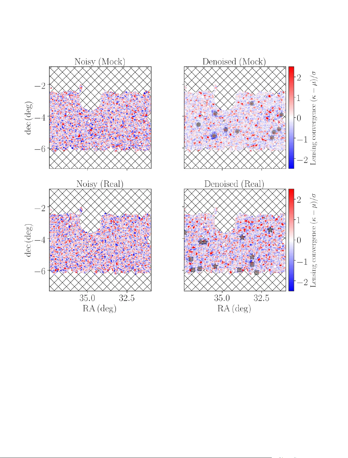
MNRAS 000 , 1 – 16 (2021) Preprint 30 August 2021 Compiled using MNRAS L A T E X sty le ﬁle v3.0 Noise reduction f or w eak lensing mass mapping: An application of g enerativ e adv ersarial netw or ks to Subaru Hyper Suprime-Cam ﬁrst-y ear data Masato Shirasaki 1 , 2 ★ Kana Moriwaki 3 , T aira Oogi 4 , N aoki Y oshida 3 , 5 , 6 , 7 , Shiro Ikeda 2 , 8 , T akahiro Nishimichi 5 , 9 , 1 National Astr onomical Observatory of Japan, Mitaka, T okyo 181-8588, Japan 2 The Institute of S tatistical Mathematics, T achikawa, T okyo 190-8562, Japan 3 Department of Physics, U niver sity of T okyo, T okyo 113-0033, Japan 4 Institute of Manag ement and Information T echnologies, Chiba U niver sity, Chiba 263-8522, Japan 5 Kavli Ins titute f or the Physics and Mat hematics of the Univ erse (WPI), Univ ersity of T okyo, Kashiw a, Chiba 277-8583, Japan 6 Institute f or Physics of Intellig ence, Univ ersity of T okyo, T okyo 113-0033, Japan 7 Resear ch Cent er for t he Early U niver se, F aculty of Science, Univ ersity of T okyo, T okyo 113-0033, Japan 8 Department of Statistical Science, Gr aduate U niver sity for Adv anced Studies, 10-3 Midori-cho, T achikawa, T okyo 190-8562, Japan 9 Center f or Gravitational Phy sics, Y ukawa Institute f or Theoretical Phy sics, K yot o Univ ersity, K yoto 606-8502, Japan ABSTRA CT W e propose a deep-learning approach based on g enerativ e adversarial networks (G ANs) to reduce noise in weak lensing mass maps under realistic conditions. W e apply imag e-to-image translation using conditional GANs to the mass map obtained from the ﬁrst-y ear data of Subar u Hyper Supr ime-Cam (HSC) surve y . W e train the conditional GANs b y using 25000 mock HSC catalogues that directl y incorporate a variety of observational eﬀects. W e study the non-Gaussian information in denoised maps using one-point probability dis tribution functions (PDFs) and also perf or m matc hing anal ysis f or positiv e peaks and massiv e clusters. An ensemble learning technique with our G ANs is successfully applied to reproduce the PDFs of the lensing con v erg ence. About 60% of the peaks in the denoised maps with height greater than 5 𝜎 hav e counter par ts of massive clus ters within a separation of 6 arcmin. W e show that PDFs in the denoised maps are not compromised by details of multiplicativ e biases and photometric redshift dis tr ibutions, nor b y shape measurement errors, and that the PDFs sho w stronger cosmological dependence compared to the noisy counter part. W e apply our denoising method to a part of the ﬁrst-y ear HSC data to sho w that the obser v ed mass distribution is statisticall y consistent with the prediction from the standard Λ CDM model. Ke y wor ds: lar ge-scale structure of U niv erse – gravitational lensing: w eak – methods: data anal ysis – cosmology : observations 1 INTR ODUCTION Impressiv e progress has been seen in observational cosmology in the past decades. An ar ray of multi-wa velength astronomical data ha ve established the standard model of our univ erse, ref erred to as Λ CDM model, with precise determination of major cosmological parameters. The nature of the main energy contents in our universe remains unknown, how ev er . Invisible mass component called dark matter is needed to e xplain the f ormation of large-scale structures in the universe ( Clo w e et al. 2004 ; A de et al. 2016 ), and an ex otic form of energy appears to be responsible f or the accelerating e xpansion of the present-day universe ( Huterer & Shaf er 2018 ). With an impor tant aim at rev ealing the nature of dark matter and the late-time cosmic acceleration, a number of astronomical surve ys are ongoing and planned. Accurate measurement of cosmic lensing shear signals is one of the pr imar y goals of such g alaxy surve ys including the Kilo-Degree Sur v ey (KiDS 1 ), the Dark Energy Surv ey ★ E-mail: masato.shirasaki@nao.ac.jp 1 http://kids.strw.leidenuniv.nl/index.php (DES 2 ), and the Subar u Hyper Suprime-Cam Surve y (HSC 3 ), ev en f or upcoming projects including the N ancy Grace R oman Space T elescope (R oman 4 ), the Leg acy Sur ve y of Space and T ime on V era C. Rubin Observatory (LSS T 5 ), and Euclid 6 . The large-scale matter distribution in the univ erse can be recon- structed through measurements of lensing shear signals by collecting and analy sing a large set of galaxy images ( T yson et al. 1990 ; Kaiser & Squires 1993 ; Schneider 1996 ). Although the image distortion of individual galaxies is typically v ery small, it is possible to inf er the distribution of under lying matter density in an unbiased wa y by av er- aging ov er many galaxies. Ho we ver , there are well-kno wn challeng es in practice when extracting r ich cosmological information from the reconstructed matter distribution. Non-linear gravitational gro wth of the larg e-scale structure renders the statistical properties of the weak 2 https://www.darkenergysurvey.org/ 3 http://hsc.mtk.nao.ac.jp/ssp/ 4 https://roman.gsfc.nasa.gov/ 5 https://www.lsst.org/ 6 http://sci.esa.int/euclid/ © 2021 The Authors 2 M. Shir asaki et al. lensing signal complicated. Numerical simulations hav e sho wn that popular and pow erful statistics for random Gaussian ﬁelds such as po wer spectr um are not able to full y descr ibe the cosmological in- f ormation impr inted in w eak lensing maps ( Jain et al. 2000 ; Hamana & Mellier 2001 ; Sato et al. 2009 ). T o e xtract and utilise the so-called non-Gaussian inf or mation, various approaches hav e been proposed (e.g. Matsubara & Jain 2001 ; Sato et al. 2001 ; Zaldarr iaga & Scocci- marro 2003 ; T akada & Jain 2003 ; Pen et al. 2003 ; Jarvis et al. 2004 ; W ang et al. 2009 ; Dietrich & Har tlap 2010 ; Kratochvil et al. 2010 ; F an et al. 2010 ; Shirasaki & Y oshida 2014 ; Lin & Kilbinger 2015 ; Petri et al. 2015 ; Coulton et al. 2018 ; Schmelzle et al. 2017 ; Gupta et al. 2018 ; Ribli et al. 2019 ), but no single statistic can capture the full information, unf or tunately . In practice, an observed w eak lensing map is contaminated with noise arising from intrinsic galaxy properties and obser vational con- ditions. The f or mer is commonly called as shape noise, which com- promises the original phy sical eﬀect. It is known that the noise eﬀect can be robustl y estimated and can also be mitigated for a Gaussian ﬁeld ( Hu & White 2001 ; Schneider et al. 2002 ), but little is kno wn about the ov erall impact of the shape noise on a non-Gaussian ﬁeld. Non-Gaussian inf or mation can potentiall y be a po werful probe to test the Λ CDM model and variant cosmological models ev en in the presence of shape noise ( Shirasaki et al. 2017a ; Liu & Madhav acheril 2019 ; Marques et al. 2019 ). For instance, Zor rilla Matilla et al. ( 2020 ) sho w that cosmological inf erence based on con v olutional neural net- w orks relies on the information car r ied by high-density regions where the noise is less impor tant. Clearl y , it is impor tant to devise a noise reduction method in order to maximise the science return from on- going and future wide-ﬁeld lensing sur v ey s. A s traightf or ward wa y of mitigating the shape noise is to smooth a w eak lensing map o v er a large angular scale (e.g. ∼ 20 − 30 arcmins in Vikram et al. ( 2015 ); Chang et al. ( 2018 )), but the smoothing it- self also erases the non-Gaussian inf ormation in the map ( Jain et al. 2000 ; T ar uya et al. 2002 ). A nov el approach has been proposed to keep a high angular resolution of ∼ 1arcmin while preserving non- Gaussian inf ormation ( Shirasaki et al. 2019b ). The method is based on a deep-learning frame work called conditional generativ e adv er - sarial netw orks (G ANs) ( Isola et al. 2016 ). Thanks to the expressiv e po wer of deep neural netw orks, conditional G ANs can denoise a w eak lensing map on a pixel-b y-pix el basis (see also Jeﬀrey et al. ( 2020 ); Rem y et al. ( 2020 ) f or similar study with a deep lear ning method). In e x chang e f or its v ersatility , deep learning methods need to be v alidated thoroughly before applied to real obser v ational data. Ho we ver , v alidation of deep learning f or lensing analyses has not been fully e xplored so far . T o ex amine and impro ve the capability of denoising with deep learning, we need to study the statis tical properties of denoised weak lensing maps using conditional GANs. In this paper, we construct and test conditional GANs and apply to the real galaxy imaging data from Subaru HSC sur v ey ( Aihara et al. 2018 ). W e use a larg e set of realistic mock HSC catalogues ( Shirasaki et al. 2019a ) to train the GANs. W e test the denoising method using 1000 test data and assess possible sys tematic errors in the denoising process. W e in ves tigate non-Gaussian inf ormation in the denoised maps by using realistic simulations of gravitational lensing. For the ﬁrst time, we ev aluate g eneralisation errors in the denoising process b y v ar ying se v eral characteristics in the moc k HSC catalogues. After stress-tes ting, we apply our GANs to the real HSC data and study the cosmological implication of the reconstr ucted large-scale matter distribution. The rest of the present paper is organised as follo ws. In Section 2 , w e summar ise the basics of gravitational lensing. Section 3 describes the HSC data as w ell as our numerical simulations used f or training and tes ting G ANs. In Section 4 , w e e xplain the details of our training strategy of GANs. Bef ore applying the GANs to the real HSC data, w e per f orm thorough tests. W e present the results in Section 5 . In Section 6 , we show the denoised map for the HSC data. Concluding remarks and discussions are given in Section 7 . 2 WEAK GRA VIT A TIONAL LENSING 2.1 Basics W e ﬁrst summarise the basics of gravitational lensing induced by the larg e-scale structure. W eak gra vitational lensing eﬀect is charac- terised by the distortion of the imag e of a source object, f ormulated b y the follo wing 2D matrix: 𝐴 𝑖 𝑗 = 𝜕 𝛽 𝑖 𝜕 𝜃 𝑗 ≡  1 − 𝜅 − 𝛾 1 − 𝛾 2 − 𝛾 2 1 − 𝜅 + 𝛾 1  , (1) where 𝜽 represents the obser v ed position of a source object, 𝜷 is the tr ue position, 𝜅 is the con ver gence, and 𝛾 is the shear. In the w eak lensing regime (i.e., 𝜅 , 𝛾  1 ), each component of 𝐴 𝑖 𝑗 can be related to the second der ivativ e of the g ra vitational potential Φ ( Bartelmann & Schneider 2001 ). Using the Poisson equation and the Born approximation, one can express the w eak lensing con v erg ence ﬁeld as the w eighted integral of matter o ver -density ﬁeld 𝛿 m ( 𝒙 ) : 𝜅 ( 𝜽 ) =  𝜒 𝐻 0 d 𝜒 𝑞 ( 𝜒 ) 𝛿 m ( 𝜒, 𝑟 ( 𝜒 ) 𝜽 ) , (2) where 𝜒 is the comoving distance, 𝜒 𝐻 is the comoving distance up to 𝑧 , and 𝑞 ( 𝜒 ) is called lensing k er nel. For a given redshift distribution of source galaxies, the lensing kernel is e xpressed as 𝑞 ( 𝜒 ) = 3 2  𝐻 0 𝑐  2 Ω m0 𝑟 ( 𝜒 ) 𝑎 ( 𝜒 )  𝜒 𝐻 𝜒 d 𝜒 0 𝑝 ( 𝜒 0 ) 𝑟 ( 𝜒 0 − 𝜒 ) 𝑟 ( 𝜒 0 ) , (3) where 𝑟 ( 𝜒 ) is the angular diameter distance and 𝑝 ( 𝜒 ) represents the redshift distribution of source galaxies nor malised to  𝜒 𝐻 0 d 𝜒 𝑝 ( 𝜒 ) = 1 . 2.2 Smoothed lensing conv ergence map In optical imaging sur v ey s, galaxies ’ shapes (ellipticities) are com- monly used to estimate the shear component 𝛾 in Eq. ( 1 ). Since each component in the tensor 𝐴 𝑖 𝑗 is given by the second der ivativ e of the gravitational potential, one can reconstruct the con v erg ence ﬁeld from the obser v ed shear , in Fourier space, as ˆ 𝜅 ( ℓ ) = ℓ 2 1 − ℓ 2 2 ℓ 2 1 + ℓ 2 2 ˆ 𝛾 1 ( ℓ ) + 2 ℓ 1 ℓ 2 ℓ 2 1 + ℓ 2 2 ˆ 𝛾 2 ( ℓ ) , (4) where ˆ 𝜅 and ˆ 𝛾 are the con ver gence and shear in Fourier space, and ℓ is the wa v e vector with components ℓ 1 and ℓ 2 ( Kaiser & Squires 1993 ). For a given source g alaxy , one considers the relation between the observed ellipticity 𝜖 obs , 𝛼 and the expected shear ˜ 𝛾 𝛼 , ˜ 𝛾 𝛼 = 𝜖 obs , 𝛼 2 R , (5) ˜ 𝛾 𝛼 = ( 1 + 𝑚 b ) 𝛾 true , 𝛼 + 𝑐 𝛼 , (6) where R is the conv ersion f actor to represent the response of the distortion of the galaxy image to a small shear ( Bernstein & Jar vis 2002 ), 𝛾 true , 𝛼 is the tr ue value of cosmic shear , and 𝑚 b and 𝑐 𝛼 are the multiplicativ e and additive biases that represent possible sys tematic MNRAS 000 , 1 – 16 (2021) Deep learning for HSC lensing map 3 uncertainty in galaxy shape measurements. In practice, bef ore em- plo ying the conv ersion in Eq. ( 4 ), one must ﬁrst construct a smoothed shear ﬁeld on gr ids ( Seitz & Schneider 1995 ), 𝛾 grid , 𝛼 ( 𝜽 ) =  𝑖 ∈ 𝜽 𝑤 𝑖  𝜖 𝑖 , obs , 𝛼 / 2 R − 𝑐 𝑖 , 𝛼  ( 1 + h 𝑚 b i )  𝑖 ∈ 𝜽 𝑤 𝑖 , (7) h 𝑚 b i =  𝑖 ∈ all 𝑤 𝑖 𝑚 b , 𝑖  𝑖 ∈ all 𝑤 𝑖 , (8) 𝛾 sm , 𝛼 ( 𝜽 ) =  d 2 𝜙 𝛾 grid , 𝛼 ( 𝝓 ) 𝑊 ( 𝝓 − 𝜽 ) (9) where 𝜽 𝑖 is the position of the 𝑖 -th source galaxy , 𝑤 𝑖 represents the in verse variance weight, and 𝑊 ( 𝜽 ) is a smoothing ﬁler . In the abov e,  𝑖 ∈ 𝜽 represents the summation o ver the galaxies in the pixel at the angular coordinate 𝜽 , while  𝑖 ∈ all is the sum o ver all the galaxies in our sur ve y windo w . In this paper, w e assume the functional f or m for 𝑊 as 𝑊 ( 𝜽 ) = 1 𝜋 𝜃 2  1 −  1 + 𝜃 2 𝜃 2 𝑠  e xp  − 𝜃 2 𝜃 2 𝑠   , (10) f or 𝜃 6 10 𝜃 𝑠 and 𝑊 ( 𝜽 ) = 0 otherwise. W e set 𝜃 𝑠 = 6 arcmins throughout this paper 7 . Using Eqs. ( 4 ) and ( 9 ), one can der iv e the smoothed con v erg ence ﬁeld from the observed imaging data through F ast Fourier T ransform (FFT). The observ ed ellipticity can be e xpressed as a sum of two ter m in practice: 𝜖 obs = 2 R 𝛾 + 𝜖 N , (11) where 𝛾 is the lensing shear of interest and 𝜖 N represents noise that originates from the intr insic galaxy shape and from obser vational conditions, ref erred to as shape noise. Accordingl y , we hav e tw o components in the observed lensing map as 𝜅 obs = 𝜅 WL + 𝜅 N . (12) The shape noise is much larg er than the lensing shear term for indi- vidual objects in typical galaxy imaging surve ys. Hence, the observed map 𝜅 obs is contaminated by the shape noise on a pixel-b y-pix el basis, which makes it challenging to extract the cosmological information contained in the map. Our objective in this paper is to estimate the noiseless ﬁeld 𝜅 WL from the observed (noisy) map 𝜅 obs . For this pur - pose, we use conditional g enerative adv ersar ial networks (GANs). 3 D A TA 3.1 Subaru Hyper Suprime-Cam Surv ey Hyper Suprime-Cam (HSC) is a wide-ﬁeld imaging camera installed at the prime focus of the 8.2-meter Subar u telescope ( Miy azaki et al. 2015 ; Aihara et al. 2018 ; K omiyama et al. 2018 ; Furusaw a et al. 2018 ; Miyazaki et al. 2018 ). The Wide Lay er in the HSC surve y will cov er 1400 deg 2 in ﬁve broad photometric bands ( 𝑔𝑟 𝑖 𝑧 𝑦 ) in its 5-y ear operation, with superb imag e quality of sub-arcsec seeing. In this paper, w e use a galaxy shape catalogue that has been produced f or cosmological weak lensing analy sis in the ﬁrst y ear data release (HSC S16A hereafter). Details of the galaxy shape measurements and catalogue information are f ound in Mandelbaum et al. ( 2018a ). 7 The smoothing scale 𝜃 𝑠 is commonly adopted to search for massive galaxy clusters in a smoothed lensing map ( Hamana et al. 2004 ). Using numer ical simulations, Shirasaki et al. ( 2015 ) has f ound a one-to-one cor respondence between the peaks on a smoothed map by the ﬁlter in Eq. ( 10 ) and massiv e galaxy clusters at 𝑧 = 0 . 1 − 0 . 3 when imposing the peak height to be larger than ∼ 5 𝜎 . In brief, the HSC S16A galaxy shape catalogue is made from the HSC Wide-La yer data taken from Marc h 2014 to April 2016 o v er 90 nights. W e use the same set of galaxies as in Mandelbaum et al. ( 2018a ) to constr uct a “secure” shape catalogue for weak lens- ing analy sis. The sky areas around br ight stars are masked ( Coupon et al. 2018 ). The HSC S16A w eak lensing shear catalogue cov ers 136.9 deg 2 that consists of the follo wing 6 disjoint patches: XMM, GAMA09H, G AMA15H, HECTOMAP , VVDS, and WIDE12H. Among the 6 patches, we choose the XMM ﬁeld as a main sample in this paper because there exis t publicl y av ailable catalogues of galaxy clusters in optical ( Ogur i et al. 2018 ) and X -ray bands ( Adami et al. 2018 ). W e can use the cluster catalogues to ex amine the reliability of our denoising process by per forming object-by -object matching. In the HSC S16A shape catalogue, the galaxy shapes are estimated using the re-Gaussianisation PSF cor rection method applied to the 𝑖 -band coadded images ( Hirata & Seljak 2003 ). In the XMM region, the surve y window is deﬁned such that 1) the number of visits within HEALPix pixels with NSIDE=1024 to be ( 𝑔 , 𝑟 , 𝑖 , 𝑧, 𝑦 ) > ( 4 , 4 , 4 , 6 , 6 ) and the 𝑖 -band limiting magnitude to be greater than 25.6, 2) the PSF modelling is suﬃciently good to meet our req uirements on PSF model size residuals and residual shear correlation functions, 3) there are no disconnected HEALPix pixels after the cut 1) and 2), and 4) the galaxies do not lie within the bright object masks. For details of deﬁning these masks, see Mandelbaum et al. ( 2018a ). The redshift distribution of the source galaxies is estimated from the HSC ﬁve broadband photometr y . T anaka et al. ( 2018 ) measure photometric redshifts (photo- 𝑧 ’ s) of the galaxies in the HSC surve y b y using sev eral diﬀerent methods. Among them, w e choose the photo- 𝑧 with a machine-learning code based on self-org anising map ( mlz ) as a baseline. T o study the impact of photo- 𝑧 estimation with diﬀerent methods, w e consider tw o additional photo- 𝑧 ’ s estimated from a classical template-ﬁtting code ( mizuki ) and a hybrid code combining machine lear ning with template ﬁtting ( frankenz ). For our analy sis, we select the source galaxies by their best estimates (see T anaka et al. ( 2018 )) of the photo- 𝑧 ’s ( 𝑧 best ) in the redshift range from 0.3 to 1.5 as done in the main cosmological analy ses f or the HSC S16A data ( Hikage et al. 2019 ). For a given method of the photo- 𝑧 estimation, individual HSC galaxies are assigned a posterior probability distr ibution function (PDF) of redshift. Figure 1 show s the stac ked PDFs for the source galaxies in the XMM. The mean source redshifts are found to be 0.96, 1.01, and 1.01 f or the estimates b y mlz , mizuki , and frankenz , respectivel y . W e then reconstruct the smoothed con ver gence ﬁeld from the HSC S16A data as described in Section 2.2 . A dopting a ﬂat-sky approxi- mation, w e ﬁrst create a pix elised shear map f or the XMM on regular gr ids with a gr id size of 1.5 arcmins. W e then appl y FFT and per f orm con volution in Fourier space to obtain the smoothed conv ergence ﬁeld. Note that we limit the maximum number of grids on a side to be 256 in our analy sis. Currently , it is still computationall y expensiv e to train GANs with larg e-size images with decent computer resources (see Brock et al. ( 2018 ) f or a recent attempt). Since our aim here is to analy se lensing conv ergence maps with an arcmin resolution, the pix el size is set to be ∼ 1 arcmin . W e will analy se observational data f or a larger region in our future w ork. Our sur ve y window co vers the range of [ 30 . 9 , 37 . 3 ] deg and [ − 7 . 29 , − 0 . 89 ] deg in r ight ascension (RA) and declination (dec), respectiv ely . There are 1345810 source galaxies av ailable with the photo- 𝑧 es timate by mlz . On the other hand, we found 1345541 and 1342017 objects for the selection based on mizuki and frankenz , respectiv ely . Note that the selection of source galaxies depends on ho w to estimate the photo- 𝑧 . In actual observations, there are missing galaxy shear data due to MNRAS 000 , 1 – 16 (2021) 4 M. Shir asaki et al. 0 . 0 0 . 5 1 . 0 1 . 5 2 . 0 2 . 5 3 . 0 Source redshift z source 0 . 000 0 . 002 0 . 004 0 . 006 0 . 008 0 . 010 Probabilit y densit y Fiducial ( mlz ) frankenz mizuki Figure 1. The stack ed photometric redshift distribution f or the galaxies in the XMM ﬁeld. The line with points show s the estimate by our baseline method, while the yello w solid and black dashed lines stand f or the results by frankenz and mizuki , respectiv ely . bright star masks. The observed regions hav e also complex geom- etry . Applying our method directl y to such regions likel y g enerates additional noises ( Shirasaki et al. 2013 ). W e determine the mask regions for each con v erg ence map b y using the smoothed number density map of the input g alaxies with the same smoothing kernel as in Eq. ( 10 ). Then we mask all the pixels with the smoothed galaxy number density less than 0.5 times the mean number density . After masking, the data region is found to co ver 21.4 deg 2 . 3.2 Mock HSC observ ations W e use a lar ge set of simulation data for training our conditional GANs. T able 1 summarises our moc k simulations. 3.2.1 F iducial simulations W e ﬁrst descr ibe the moc k shape catalogues f or HSC S16A. The mock catalogues are generated from 108 full-sky lensing simulations presented in T akahashi et al. ( 2017 ) 8 . In T akahashi et al. ( 2017 ), the authors perform a suite of cosmological 𝑁 -body simulations with 2048 3 particles and generate lensing con v erg ence maps and halo catalogues. The 𝑁 -body simulations assume the standard Λ CDM cosmology consistent with the 9-y ear WMAP cosmology (WMAP9) ( Hinsha w et al. 2013 ) with the CDM density parameter Ω cdm = 0 . 233 , the baryon density Ω b0 = 0 . 046 , the matter density Ω m0 = Ω cdm + Ω b0 = 0 . 279 , the cosmological constant Ω Λ = 0 . 721 , the Hubble parameter ℎ = 0 . 7 , the amplitude of density ﬂuctuations 𝜎 8 = 0 . 82 , and the spectral index 𝑛 𝑠 = 0 . 97 . The gravitational lensing eﬀect is simulated with the multiple lens-plane algor ithm on a curved sky ( Becker 2013 ; Shirasaki et al. 2015 ). Light-ray deﬂection is directly f ollow ed by using the projected matter density ﬁeld produced b y the outputs from the 𝑁 -body simulations. Each lensing simulation data consists of 38 diﬀerent source planes at redshift less than 5.3. Realis tic source redshift distributions are implemented f ollo wing the curves in Figure 1 . 8 The full-sky light-cone simulation data are freel y a vailable f or do wn- load at http://cosmo.phys.hirosaki- u.ac.jp/takahasi/allsky_ raytracing/ . T o generate mock shape catalogues, we emplo y essentially the same method as dev eloped in Shirasaki & Y oshida ( 2014 ); Shirasaki et al. ( 2017b ). W e use the full-sky simulations combined with the observed photometric redshifts and angular positions of real galaxies. Pro vided the real catalogue of source galaxies, where each galaxy contains inf ormation on the position (RA and Dec), shape, redshift, and the lensing w eight, w e perf or m the f ollowing f our -steps: (i) Set the RA and Dec of the surve y window in the full-sky reali- sation. (ii) Populate source galaxies on the light-cone using or iginal angu- lar positions and redshifts of the observed galaxies. (iii) Rotate the shape of each source g alaxy at random to erase the real lensing signal. (iv) Add the lensing shear on each source galaxy using the lensing simulations In the step (ii), w e dra w the source redshift at random b y f ollowing the pos ter ior distribution of photo- 𝑧 estimates on an object-by -object basis. Hence, our mock catalogue contains galaxies at 𝑧 < 0 . 3 or 𝑧 > 1 . 5 . Note that our method maintains the obser v ed proper ties of the source galaxies on the sky . W e increase the number of realisations of the mock catalogues by extracting multiple separate regions from a single full-sky simulation. Finally we obtain 2268 mock catalogues in total 9 . 3.2.2 Photome tric redshift uncertainties In the ﬁducial moc k catalogues, we utilise the photo- 𝑧 inf or ma- tion estimated b y mlz . T o e xamine possible systematic eﬀects o wing to photo- 𝑧 uncertainties, we generate additional moc k realisations adopting the tw o other redshift estimates by mizuki or frankenz . W e produce 100 mock realisations of the HSC S16A catalogues for each model, and use them to ev aluate the impact of photo- 𝑧 uncer- tainty in our denoising process. 3.2.3 Imag e calibration uncertainties W e use a single value of multiplicative bias h 𝑚 b i (deﬁned in Eq. [ 8 ]) when generating our ﬁducial mock catalogues. Estimating h 𝑚 b i is based on image simulations, and thus there remains a 1% -le vel uncer - tainty ( Mandelbaum et al. 2018b ). T o account f or possible sys tematic eﬀects by the mis-estimation of the multiplicative bias, we make ad- ditional mock realisations by changing h 𝑚 b i → h 𝑚 b i + Δ 𝑚 b in the production process. W e assume tw o values of Δ 𝑚 b = ± 0 . 01 . F or each value of Δ 𝑚 b , we produce 100 mock realisations of the HSC S16A. 3.2.4 Noise model uncertainties Imperfect kno wledg e of the noise distribution in the data can be another source of sys tematic uncer tainties in denoising process. T o assess possible model bias in the noise, we generate tw o diﬀerent mock catalogues by varying the amplitude of the standard deviation (error) of the shape measurement, 𝜎 mea . In the HSC S16A data, the value of 𝜎 mea has been calibrated with a set of image simulations, and the es timate f or individual objects ma y be subject to a 10% -le vel uncertainty ( Mandelbaum et al. 2018b ). T o test the impact of this uncertainty , we v ar y the amplitude of 𝜎 mea b y a f actor of ( 1 + Δ 𝜎 mea ) 9 The mock shape catalogues are publicl y a vailable at http://gfarm. ipmu.jp/~surhud/ . MNRAS 000 , 1 – 16 (2021) Deep learning for HSC lensing map 5 T able 1. Summary of our mock catalogues for Subaru Hyper -Supr ime Cam Surve y ﬁrst-year data. For each of 100 cosmological models (parameter sets), we hav e 50 realisations of mock catalogues. Name # of realisations Cosmology Note Ref erence Fiducial 2268 WMAP9 cosmology ( Hinshaw et al. 2013 ) Photo- 𝑧 info by mlz Section 3.2.1 Photo- 𝑧 run 1 100 - Photo- 𝑧 info by mizuki Section 3.2.2 Photo- 𝑧 run 2 100 - Photo- 𝑧 info by frankenz - multiplicativ e-bias run 1 100 - Change h 𝑚 b i b y + 0 . 01 Section 3.2.3 multiplicativ e-bias run 2 100 - Change h 𝑚 b i b y − 0 . 01 - Noise-v aried r un 1 100 - Change 𝜎 mea by + 10% Section 3.2.4 Noise-v aried r un 2 100 - Change 𝜎 mea by − 10% - Cosmology-v ar ied r un 50 × 100 100 diﬀerent models (Figure 2 ) Photo- 𝑧 info b y mlz Section 3.2.5 on an object-by -object basis when generating mock catalogues. W e keep the lensing w eight ﬁxed e v en when varying 𝜎 mea in the lensing analy sis, because w e suppose that w e are unaw are of the mis-estimate of 𝜎 mea . W e assume two values, Δ 𝜎 mea = 0 . 1 and Δ 𝜎 mea = − 0 . 1 . For each value of Δ 𝜎 mea , we produce 100 mock realisations of the HSC S16A. 3.2.5 V ar ying cosmological models T o study the cosmological dependence on weak lensing maps, w e also generate mock catalogues of the HSC S16A data b y varying cosmological models. W e design the cosmological models f or simu- lations so as to co ver a much wider area in the tw o-parameter space ( Ω m0 , 𝜎 8 ) than the constraints by the cur rent galaxy imaging sur - v ey s ( Hildebrandt et al. 2017 ; T ro xel et al. 2018b , a ; Hikage et al. 2019 ). W e choose a sample of cosmological models in the Ω m0 − 𝜎 8 plane by using a public R package to generate the maximum-distance sliced Latin Hypercube Designs (LHDs) ( Ba et al. 2015 ). W e ﬁrst generate 120 designs in a two dimensional rectangle speciﬁed by 0 . 1 6 Ω m0 6 0 . 7 and 0 . 4 6 𝜎 8 ( Ω m0 / 0 . 3 ) 0 . 6 6 1 . 1 using the codes. W e then restrict the designs to those with 0 . 4 6 𝜎 8 6 1 . 4 . This lea ves 100 designs. Figure 2 sho ws the resultant 100 cosmologi- cal models adopted in our simulations. Note that we set Ω Λ = 1 − Ω m0 assuming a spatially ﬂat universe. For other parameters, we adopt Ω b0 ℎ 2 = 0 . 02225 , ℎ = 0 . 6727 and 𝑛 𝑠 = 0 . 9645 . These parameters are consistent with the results from Planck 2015 ( Ade et al. 2016 ). For each cosmological model, w e per f or m ray -tracing simulations under a ﬂat-sky approximation. W e adopt the multiple lens-plane algorithm ( Jain et al. 2000 ; Hamana & Mellier 2001 ) to simulate the gravitational lensing eﬀects on a light cone of angular size 10 ◦ × 10 ◦ . W e place a set of 𝑁 -body simulations with diﬀerent volumes to co ver a wide redshift rang e as well as ha ve higher mass and spatial resolutions at low er redshifts (e.g. see, Sato et al. ( 2009 )). W e consider four diﬀerent box sizes on a side and each box size is varied as a function of the cosmological model. The bo x size 𝐿 bo x of the 𝑁 -body simulations f or our ra y-tracing simulations is set by the f ollo wing criter ia: 𝐿 bo x , 1 = 𝜒 ( 𝑧 = 0 . 5 ) × ( 𝜃 sim + Δ 𝜃 ) , (13) 𝐿 bo x , 2 = 𝜒 ( 𝑧 = 0 . 8 ) × ( 𝜃 sim + Δ 𝜃 ) , (14) 𝐿 bo x , 3 = 𝜒 ( 𝑧 = 1 . 5 ) × ( 𝜃 sim + Δ 𝜃 ) , (15) 𝐿 bo x , 4 = 𝜒 ( 𝑧 = 3 . 0 ) × ( 𝜃 sim + Δ 𝜃 ) , (16) where 𝐿 bo x , 𝑖 is the box size f or the 𝑖 -th smallest-v olume simulation and 𝜃 sim = 10 deg . W e introduce the buﬀer in opening angle to com- pute 𝐿 bo x and set Δ 𝜃 = 2 deg . W e then place the 𝑁 -body simulations 0 . 2 0 . 4 0 . 6 Ω m0 0 . 4 0 . 6 0 . 8 1 . 0 S 8 = σ 8 (Ω m0 / 0 . 3) 0 . 5 Figure 2. The 100 diﬀerent cosmological models to study the cosmological dependence on weak lensing maps. At each point, we generate 50 mock realisations of the HSC S16A data. with the bo x size of 𝐿 bo x , 1 , 𝐿 bo x , 2 , 𝐿 bo x , 3 and 𝐿 bo x , 4 to cov er the light cone in the redshift range of 0 < 𝑧 < 0 . 5 , 0 . 5 < 𝑧 < 0 . 8 , 0 . 8 < 𝑧 < 1 . 5 , and 1 . 5 < 𝑧 < 3 . 0 , respectivel y . F igure 3 sho ws an ex ample of the conﬁguration of 𝑁 -body box es in our ray -tracing simulation in the case of Ω m0 = 0 . 3 . For a given single 𝑁 -body simulation volume, w e produce two sets of the projected density ﬁelds with a projection depth of 𝐿 bo x / 2 on 9600 2 gr ids by using the tr iangular -shaped cloud assignment scheme ( Press et al. 1992 ). By sol ving the discretised lens equation numerically , we obtain the lensing con ver gence 𝜅 and shear 𝛾 on 4096 2 gr ids with a g rid size of 0.15 arcmin. A single realisation of our ra y-tracing data consists of 22 source planes in the range of 𝑧 < ∼ 3 . W e perform 50 ray -tracing realisations of the under lying density ﬁeld b y randomly shifting the simulation bo x es assuming periodic boundary conditions. W e ﬁnally produce the mock catalogue of the HSC S16A as descr ibed in Sec 3.2.1 . When running cosmological 𝑁 -body simulations, w e use the par - allel T ree-Par ticle Mesh code GADGET2 ( Springel 2005 ). W e generate the initial conditions using a parallel code dev eloped b y Nishimichi et al. ( 2009 ); V alageas & Nishimichi ( 2011 ), which employ the second-order Lagrangian perturbation theory ( Crocce et al. 2006 ). The number of 𝑁 -body par ticles is set to 512 3 . W e set the initial redshift b y 1 + 𝑧 init = 36 ( 512 / 𝐿 bo x ) , where we compute the linear matter transfer function using CAMB ( Lewis et al. 2000 ). Note that MNRAS 000 , 1 – 16 (2021) 6 M. Shir asaki et al. Figure 3. The conﬁguration of 𝑁 -body bo xes in our ra y-tracing simulation f or the cosmology with Ω m0 = 0 . 3 . our choice of the initial redshift is motiv ated by the detailed study of Nishimichi et al. ( 2019 ). 4 DENOISIN G B Y DEEP -LEARNING NETW ORKS 4.1 Conditional generative adv ersarial netw orks T o perform mapping from a noisy lensing ﬁeld 𝜅 obs to a noiseless counterpar t 𝜅 WL , we use a model of conditional generativ e adver - sarial networks dev eloped in Isola et al. ( 2016 ). The networks ha ve tw o main components, a generator and a discriminator . W e train the netw orks so that the generator applies some transformation to the input noisy ﬁeld 𝜅 obs to output a noise ﬁeld 𝜅 N 10 . The discriminator compares the input image to an unkno wn image (either a target image from the data set or an output image from the generator) and tr ies to judge if it is produced by the generator . T o be speciﬁc, the input image f or the discr iminator is set to the noisy ﬁeld 𝜅 obs , while the targ et image is either of the noise counter par t of 𝜅 obs or an output from the generator . The structure of the g enerator and the discr iminator in our net- w orks is essentially the same as in Shirasaki et al. ( 2019b ), ex cept f or minor parameter tuning. The generator uses a U-Net str ucture ( R onneberg er et al. 2015 ) with an eight set of conv olution and de- con volution la yers. Each conv olution la yer consists of con v olution with a kernel size of 5 × 5 , the batch normalisation, and the appli- cation of the activation function of leaky ReL U with a leak slope of 0.2. The deconv olution lay er does the inv erse operation of the con volution lay er . The generator also has additional skip connec- tions between mirror lay ers to propagate the small-scale inf ormation that would be lost as the size of the images decreases through the con volution process. The discriminator produces a single value from a giv en input image for the decision whether the input is real or a 10 One ma y think that it would be more appropriate to directly generate a noiseless lensing ﬁeld in the network. This possibility has been ex amined in our previous work and it does not w ork in an HSC-like imaging surve y ( Shirasaki et al. 2019b ). This is mainly because the signal-to-noise ratio on a pixel-b y-pix el basis is small in general. fak e. The ﬁnal output of the discr iminator is made after the image reduction through 4 conv olution lay ers and after av eraging all the responses from the con volution la y ers. In the conv olution lay ers in the discriminator , w e remo ve the batch nor malization to balance the losses of the g enerator and the discriminator in a stable wa y . The resulting number of parameters in our netw orks is close to 400000. 4.2 T raining the networ ks The objectiv e of our networks is to solv e an optimization problem with a cost function e xpressed as a combination of loss functions as min 𝐺 max 𝐷  L cGAN ( 𝐺 , 𝐷 ) + 𝜆 L L1  , (17) where 𝐺 indicates the generator and 𝐷 is the discriminator . W e here introduce two loss functions as L cGAN ( 𝐺 , 𝐷 ) = E 𝑥 , 𝑦 log 𝐷 ( 𝑥 , 𝑦 ) + E 𝑥 , 𝑧 log { 1 − 𝐷 ( 𝑥 , 𝐺 ( 𝑥 , 𝑧 ) ) } , (18) L L1 ( 𝐺 ) = E 𝑥 , 𝑦 , 𝑧  map | 𝑦 − 𝐺 ( 𝑥 , 𝑧 ) | , (19) where 𝑥 is the input noisy ﬁeld, 𝑦 is the true noise ﬁeld, and 𝑧 is a random noise v ector at the bottom lay er of the generator . The function 𝐷 ( 𝑋 1 , 𝑋 2 ) retur ns the score in the range of zero to unity to ev aluate if the noise counter par t of 𝑋 1 and a noise ﬁeld 𝑋 2 are identical or not. In Eq. ( 19 ), the summation runs ov er all the pixels in a map but with the masked region ex cluded. In the training, we alternate between one g radient descent step on 𝐷 , then one step on 𝐺 . As suggested in Goodfello w et al. ( 2014 ), w e train to maximise the term of log 𝐷 ( 𝑥 , 𝐺 ( 𝑥 , 𝑧 ) ) . Also, we divide the objectiv e b y 2 while optimising 𝐷 , which slow s down the lear ning rate of 𝐷 relative to 𝐺 . When training the networks, we use the minibatch Stoc hastic Gra- dient Descent (SGD) method and apply the A dam solv er ( Kingma & Ba 2014 ), with lear ning rate 0 . 0002 , momentum parameters 𝛽 1 = 0 . 5 and 𝛽 2 = 0 . 9999 . W e also set 𝜆 = 75 in Eq. ( 17 ). The parameter 𝜆 controls the strength of the regularisation given by the L1 norm. All the netw orks in this paper are trained with a batc h size of 1. W e initialise the model parameters in the networks from a Gaussian distribution with a mean 0 and a standard de viation of 0 . 02 . W e train our networks using the T ensorFlo w implementation 11 on a sin- gle NVIDIA Quadro P5000 GPU. While processing, we randomly select training and validation data from the input data sets. Each netw ork is validated ev ery time it lear ns 100 image pairs. T o prepare the training data set, we use 400 realisations of our mock HSC S16A catalogues (Section 3.2.1 ). Using the information of noiseless lensing maps 𝜅 and 𝛾 in our surve y windo w , w e gener - ate 60000 noisy maps b y injecting independent noise realizations at random. From the 60000 image pairs of the noisy ﬁeld 𝜅 obs and the underl ying noise 𝜅 N , we select 25000 image pairs b y bootstrap sam- pling so that each bootstrap realisation can contain 167 realisations of noiseless lensing ﬁelds. In our previous study , we ﬁnd that it is near -optimal to use ∼ 200 realisations of noiseless lensing ﬁelds and set the number of training sets to ∼ 30000 for our networks ( Shirasaki et al. 2019b ). T o set the hyperparameter in our network, we examined the training with 𝜆 = 25 , 50 , 75 , 100 , and 150 . For a giv en 𝜆 , w e v ar ied the number of image pairs in the training process from 20000 to 40000 11 W e use the modiﬁed version of https://github.com/yenchenlin/ pix2pix- tensorflow MNRAS 000 , 1 – 16 (2021) Deep learning for HSC lensing map 7 Figure 4. An example of image-to-imag e translation by our netw orks. The left panel show s an input noisy lensing map, while the right stands for the true (noiseless) counter par t. The medium represents the reconstructed map by our conditional GANs. For the reconstructed map, we ﬁrst obtain the under lying noise ﬁeld from 10 bootstrap realisations of the generators in our GANs and then derive the conv erg ence map by the residual between the input noisy map and the predicted noise. In this ﬁgure, the hatched region show s the masked area due to the presence of bright stars and inhomog eneous angular distributions of galaxies in our surve y windo w . In the legend, 𝜇 and 𝜎 denote the spatial a verag e and the root-mean-square of lensing ﬁelds, respectivel y . at inter vals of 5000. W e then apply the netw ork trained with diﬀerent h yper parameters to the test sets. After some tr ials, we ﬁnd that the training with 25000 image pairs and 𝜆 = 75 can provide the best performance on noise reduction in the test sets. 4.3 Production of the ﬁnal denoised image As repor ted in Shirasaki et al. ( 2019b ), a single set of our netw orks trained by 25000 imag e pairs has a larg e scatter in the image-to- image translation. T o reduce this dependence on training data sets, w e generate 10 bootstrap sampling of 25000 training data and obtain a total 10 networks f or denoising. Namel y , we obtain 10 candidates of the underl ying noise ﬁeld 𝜅 N f or a given noisy ﬁeld 𝜅 obs . T o ev aluate the best estimate of 𝜅 N , we take the median o ver the 10 candidates on a pixel-b y-pix el basis. Once the av eraged estimate of 𝜅 N is determined in this manner, we evaluate the underlying noiseless ﬁeld 𝜅 WL b y subtracting the best noise model from the obser ved one 𝜅 obs . The denoising process by our networks is tested by 1000 noisy data from the ﬁducial mock catalogues. These test data are not used in the training process. 5 PR OPERTIES OF DENOISED MAPS In this section, we s tudy statistical proper ties of w eak lensing maps denoised b y our conditional G ANs. W e pa y special attention to non-Gaussian inf ormation in the maps. In this paper, we consider one-point distr ibution function (PDF) to e xtract non-Gaussian in- f ormation. Fur thermore, we emplo y matching analy ses of peaks in the maps and massive clusters in the N-body simulations, demon- strating that our GANs do not erase r ich cosmological information from high-density regions. In Appendix A , we summar ise additional tests f or our GANs. The tests include a conv entional two-point cor - relation analy sis, a reliability chec k of our G ANs ’ predictions, and dependence of our results on hyperparameter in our GANs. Our training strategy for conditional G ANs is pro vided in Sec- tion 4 . Here, w e show the validation results of the outputs from our netw orks by using 1000 test data sets. These test sets are based on the ﬁducial mock catalogues as in Section 3.2.1 , while we do not use them in the training process. In the f ollo wing, the lensing map is normalised so as to hav e zero mean and unit variance. 5.1 Visual comparison A quic k visual comparison would allo w us to highlight how our GAN-based denoising w orks for noisy input images. Figure 4 com- pares three maps f or one of our test data. In the ﬁgure, the left and right panels sho w an input noisy and the true noiseless counter par t, respectiv ely . The middle panel show s the denoised map b y our condi- tional GANs. In each panel, red spots indicate high density regions, while bluer ones hav e low er densities. The denoised imag e retains similar patter ns in density contrast o ver a fe w degrees compared to the ground tr uth. Note that Figure 4 concentrates on the pix el v alues in the range of − 2 . 5 𝜎 to + 2 . 5 𝜎 , i.e., largel y noise dominated. Although not perf ect, our G ANs reco ver small-scale inf ormation (e.g., positiv e peaks) closely to the ground truth. 5.2 One-point probability distribution One-point PDF is a simple summary statistic of a w eak lensing map. Our previous study show s that the denoised image yields a similar PDF to the noiseless tr ue counter par t if the lensing ﬁeld is properl y normalised ( Shirasaki et al. 2019b ). Here, we repeat the previous analy sis but with including various observ ational eﬀects such as comple x surve y geometry , inhomogeneous galaxy distribution on a sky , wide redshift distribution of source galaxies, and variation of MNRAS 000 , 1 – 16 (2021) 8 M. Shir asaki et al. 10 − 3 10 − 2 10 − 1 10 0 One-p oin t PDF P T raining (25K sets) T ruth Noisy Denoised − 2 0 2 4 ( κ − µ ) /σ − 1 0 1 ∆ P / Err[ P ] Figure 5. W e compare the lensing PDFs for noisy , noiseless and denoised maps. The solid line in the top panel sho ws the av eraged PDF ov er the 1000 noiseless lensing maps, while the dashed line is f or the noisy (observed) one. The red points in the top panel sho w the av eraged PDF f or the denoised maps by our GANs. In the bottom, we show the diﬀerence between the noiseless and denoised PDFs nor malised by the sample variance of the noiseless PDFs. For reference, we highlight ± 0 . 5 𝜎 -lev el diﬀerences by the mag enta lines at the bottom. the weights in the analy sis. For a given lensing map, we measure the one-point PDF as a function of ( 𝜅 − 𝜇 ) / 𝜎 where 𝜇 and 𝜎 are the spatial av erage and the root-mean-square. W e per f orm linearl y spaced binning in the rang e of − 15 < ( 𝜅 − 𝜇 ) / 𝜎 < 15 with width of 0.3. Figure 5 compares the PDFs av eraged o v er 1000 realisations of lensing ﬁelds. The noiseless PDF is signiﬁcantl y ske wed compared to the observed noisy counter par ts. Our method reproduces the larg e ske wness in the noiseless PDFs from the noisy input images. The typical bias in the reconstruction ranges from a 0 . 5 − 1 𝜎 lev el ov er a wide range of pixel values as sho wn in the bottom panel. 5.3 P eak -halo matching T o study the small-scale str ucture on a denoised lensing ﬁeld, w e e xamine the cor respondence between dark matter haloes and the local maxima in the lensing maps. Since our mock HSC catalogues are or iginally based on cosmological 𝑁 -body simulations, we can generate light-cone halo catalogues with the same sky co verag e as the lensing maps. The light-cone catalogues are produced from the inherent full-sky halo catalogues of T akahashi et al. ( 2017 ). The dark matter haloes in the full-sky catalogues are identiﬁed b y a phase-space temporal halo ﬁnder Rockstar ( Behroozi et al. 2013 ). In the follo wing, w e consider two mock cluster catalogues; one is a simple mass-limited sample, and the other takes into account a realis- tic mass selection eﬀect in optically -selected galaxy clusters. F or the mass-limited sample, we use dark matter haloes with mass 12 greater than 10 14 ℎ − 1 𝑀  at redshift less than 1. The mass and redshift selec- tion roughly cor responds to the real galaxy cluster catalogue based 12 W e deﬁne the halo mass as the spher ical o ver -density mass with respect to 200 times mean o ver -density . on the photometr ic data in HSC S16A ( Ogur i et al. 2018 ). In order to use more realistic samples, we g enerate mock galaxy clusters based on the multi-band identiﬁcation of red sequence g alaxies (the cluster ﬁnding algorithm is referred to as CAMIRA; Ogur i 2014 ). W e adopt the mass-to-richness relations of the C AMIRA clusters identiﬁed in HSC S16A ( Murata et al. 2019 ). Murata et al. ( 2019 ) assume a log- normal distribution of the cluster r ichness for giv en cluster masses and redshifts and constrain the mean and scatter relation between the cluster mass and richness. Using their log-nor mal model, we assign the cluster richness to dark matter haloes in their redshift range of 0.1 to 1.0. In a given lensing map, w e ﬁrst identify local maxima with their peak heights greater than 5 𝜎 . W e then search for clus ters around the peaks with a search radius of 6 arcmins. When we ﬁnd se veral haloes in the search radius, w e regard the closest cluster from the position of the peak as the best match. Over 1000 realisations in our sur v ey windo w , w e ﬁnd 27683 peaks. W e identify 89 . 5% of the peaks hav e a matched mass-limited cluster in the noiseless ﬁeld. After denoising, the number of peaks is f ound to be 23248 and the matching rate is 64 . 6% . For more realistic CAMIRA -like clusters, the matching rate is found to be 85 . 1% and 58 . 9% for the noiseless and denoised ﬁelds, respectivel y . Without denoising, the number of peaks reduces to 1669 ov er 1000 realisations. How ev er , the matching rate is f ound to be 80 . 2% and 75 . 2% for the mass-limited and the CAMIRA -like clusters, respectiv ely . Hence, the anal ysis with denoising is highly complementary to the noisy counter part. Further more, to v alidate the halo-peak matc hing, w e study the number density of the matched dark matter haloes as a function of halo masses and redshifts. Figures 6 and 7 sho w the number density of the matched clusters to the noiseless, the denoised, and the noisy peaks. As shown in the ﬁgures, the shape of the number density looks similar betw een the noiseless and the denoised peaks. This indicates that the peak -cluster matching f or the denoised ﬁelds is not a coincidence. Compared to the noisy peaks, the denoised peaks pla y an impor tant role to search f or less massiv e clusters. 5.4 Cosmological dependence on lensing PDFs W e next validate if our conditional GANs can reduce noises when the true cosmologocal model is diﬀerent from that assumed in the training process. When our GANs would surely lear n noise proper ties alone, the networks should be able to denoise regardless of underl ying cosmological models. T o study the cosmological dependence on the denoised lensing map, w e use the mock catalogues as in Section 3.2.5 . W e hav e 50 mock realisations of noisy lensing maps f or each of 100 diﬀerent cosmological models. For a given cosmology , we input a noisy map to our GANs, obtain the denoised map, and then compute the one-point PDF from the denoised map. W e repeat this process f or 50 realisations per each cosmological model and estimate the a verag e PDF . Figure 8 summar ises the cosmological dependence on the de- noised PDF f or the HSC S16A. W e ﬁnd a clear dependence of the cosmological model, highlighting that our GANs do not ov er ﬁt to the assumed cosmology in the training. The results in Figure 8 can be compared with the PDFs for noisy input maps. The cosmological dependence of the lensing PDFs without our denoising is sho wn in Figure 9 . This illustrates that the cosmological dependence is w eak compared to the s tatistical error of the PDF when one w orks on the original noisy lensing map. Our results indicate that the denoised PDF would potentiall y constrain the cosmological parameters tighter than the noisy counter par t does. How ev er , the denoised PDFs are less sensitiv e to the cosmological parameters than the noiseless counter - MNRAS 000 , 1 – 16 (2021) Deep learning for HSC lensing map 9 10 14 10 15 10 − 5 10 − 4 10 − 3 10 − 2 10 − 1 10 0 Num b er densit y [deg − 2 ] 0 . 2 ≤ z < 0 . 4 10 14 10 15 M 200b [ h − 1 M  ] 0 . 4 ≤ z < 0 . 6 10 14 10 15 0 . 6 ≤ z < 0 . 8 T ruth ( × 0 . 7) T ruth Denoised Noisy Figure 6. The number density of the matched dark matter haloes to the peaks on the lensing peaks. From the left to the right, w e show the number density of the dark matter haloes as a function of halo masses 𝑀 200b at three diﬀerent redshift ranges, 0 . 2 6 𝑧 < 0 . 4 , 0 . 4 6 𝑧 < 0 . 6 , and 0 . 6 6 𝑧 < 0 . 8 . The grey histogram sho ws the results for the tr ue (noiseless) lensing ﬁelds, while the red points and green squares stand for the denoised and noisy ﬁelds, respectivel y . The red points broadly follo w the grey histogram e x cept for the diﬀerence in amplitudes. For a reference, the dashed line in each panel represents the noiseless results with a multiplicativ e factor of 0.7. 10 2 10 − 5 10 − 4 10 − 3 10 − 2 10 − 1 10 0 Num b er densit y [deg − 2 ] 0 . 2 ≤ z < 0 . 4 10 2 Cluster ric hness R 0 . 4 ≤ z < 0 . 6 10 2 0 . 6 ≤ z < 0 . 8 T ruth ( × 0 . 7) T ruth Denoised Noisy Figure 7. Similar to Figure 6 , but we sho w the peak -cluster matching results f or the CAMIRA-lik e mock catalogues. parts (see Figure 10 ). In addition, the noiseless PDF is f ound to be larg ely sensitiv e to the parameter of 𝜎 8 ( Ω m0 / 0 . 3 ) 0 . 2 − 0 . 3 , while the denoised and noisy PDFs are mainly deter mined by 𝜎 8 ( Ω m0 / 0 . 3 ) 0 . 5 . A ccording to these diﬀerences, the cosmological inf ormation in de- noised PDFs is not identical to that in true PDFs. W e need additional analy ses to study the information content in the denoised PDFs and its relation with other statis tics (e.g. Shirasaki 2017 ). W e lea v e those f or our future study . 5.5 A ccounting f or sy stematic uncertainties W e here discuss g eneralisation er rors in the denoising based on our GANs. T o quantify the er rors, we introduce a simple c hi-squared statis tic f or denoised lensing PDFs: Δ 𝜒 2 =  𝑖 , 𝑗 [ P 𝑖 ( test ) − P 𝑖 ( ﬁd ) ] 𝑪 − 1 𝑖 𝑗  P 𝑗 ( test ) − P 𝑗 ( ﬁd )  , (20) where P 𝑖 ( test ) is the denoised PDF at the 𝑖 -th bin under our ﬁdu- cial cosmological model but including diﬀerent sys tematic eﬀects in galaxy shape measurements, P ( ﬁd ) is the denoised PDF for our ﬁdu- MNRAS 000 , 1 – 16 (2021) 10 M. Shir asaki et al. 10 − 3 10 − 2 10 − 1 10 0 One-p oin t PDF P Denoised (T rained b y 25K sets) Fiducial − 2 0 2 4 ( κ − µ ) /σ − 2 . 5 0 . 0 2 . 5 ∆ P / Err[ P ] 0 . 25 0 . 50 Ω m0 0 . 5 1 . 0 σ 8 Figure 8. The cosmological dependence of the one-point PDF of the denoised maps. The top panel show s the PDF as a function of the pix el value ( 𝜅 − 𝜇 ) / 𝜎 , where 𝜇 and 𝜎 is the spatial a v erage and root-mean-square for a lensing ﬁeld 𝜅 , respectivel y . In the top, the inset ﬁgure represents the 100 cosmological models considered in the present study . The star symbol in the inset ﬁgure sho ws our ﬁducial model (the WMAP9 cosmology; Hinshaw et al. 2013 ). The dependence of cosmological models is highlighted by the colour diﬀerence. In the bottom, we show the diﬀerence of the PDF from our ﬁducial cosmological model normalised by the statis tical uncertainty . 10 − 3 10 − 2 10 − 1 10 0 One-p oin t PDF P Noisy Fiducial − 2 0 2 4 ( κ − µ ) /σ − 2 . 5 0 . 0 2 . 5 ∆ P / Err[ P ] 0 . 25 0 . 50 Ω m0 0 . 5 1 . 0 σ 8 Figure 9. Similar to Figure 8 , but for the lensing PDF without our denoising process. cial model, and 𝑪 represents the cov ariance matr ix f or the denoised PDF . W e e valuate P ( test ) b y the a v erage o v er 100 realisations shown in Sections 3.2.2 , 3.2.3 , and 3.2.4 . Similarly , we compute P ( ﬁd ) by a veraging 1000 test data set in our ﬁducial r un and estimate 𝑪 from 1000 test realisations in our ﬁducial r un. Bef ore sho wing results, w e caution the limitation of our approach. All the analy ses in this paper assume the bar yonic eﬀects on the cosmic mass density can be negligible. Osato et al. ( 2015 ); Castro 10 − 3 10 − 2 10 − 1 10 0 One-p oin t PDF P Noiseless Fiducial − 2 0 2 4 ( κ − µ ) /σ − 5 0 5 ∆ P / Err[ P ] 0 . 25 0 . 50 Ω m0 0 . 5 1 . 0 σ 8 Figure 10. Similar to Figure 8 , but f or the lensing PDF in the absence of shape noises. et al. ( 2018 ) e xamined the bar yonic eﬀects on the lensing PDF with h ydrodynamical simulations and found the most prominent eﬀect w ould appear in high- 𝜎 tails in the PDF . This is because the bar y- onic eﬀects such as cooling, star f ormation, and feedbac k from activ e galactic nuclei commonly play a cr itical role in high-mass-density en vironments in the univ erse. Besides, we ignore possible cor rela- tions between the lensing shear and the shape noises. An example causing such correlations is the intrinsic alignment (IA) ( Tro xel & Ishak 2014 ). Although this IA eﬀect can potentially cause the biased parameter estimation in future sur v ey s ( Krause et al. 2016 ), we ex- pect it would be less important for our analy sis because we do not emplo y cluster ing analyses of galaxy shapes. According to the ob- servational f acts, the IA eﬀect is expected to be more prominent f or redder galaxies (e.g. see Hirata et al. ( 2007 )). Since redder galaxies pref erentially reside in denser environments such as galaxy clusters, w e would mitigate the impact of the IA eﬀect on our analy sis when remo ving the high- 𝜎 inf ormation. T o take into account these eﬀects, w e decide to remo v e such high-density regions b y setting the rang e of pix el values to be P > 0 . 01 in Eq. ( 20 ). This lea ves the lensing PDF at − 2 . 1 < ( 𝜅 − 𝜇 ) / 𝜎 < 3 . 3 with the number of bins being 18. In this setup, we would argue that there exist signiﬁcant generalisation errors in our denoising when ﬁnding Δ 𝜒 2 > √ 2 × 18 = 6 . 5.5.1 Photome tric redshifts With our GANs, we assume the source redshift estimation by the speciﬁc mlz method, but other methods predict the diﬀerent redshift distributions accordingl y (see Figure 1 ). T o assess the sy stematic un- certainty due to imperfect photo- 𝑧 estimates, we compute Eq. ( 20 ) when setting the ter m of P ( test ) to be the av eraged PDF o ver 100 re- alisations of the mock catalogues with diﬀerent photo- 𝑧 inf or mation (Sec 3.2.2 ). W e ﬁnd that the photo- 𝑧 estimate by diﬀerent methods can induce the bias in the lensing PDFs with a < ∼ 0 . 3 𝜎 lev el ov er a wide range of pixel values. These diﬀerences introduce Δ 𝜒 2 = 0 . 290 and 0 . 134 f or the Photo- 𝑧 run 1 and 2, respectiv ely . MNRAS 000 , 1 – 16 (2021) Deep learning for HSC lensing map 11 5.5.2 Multiplicativ e bias Besides, we assume the multiplicativ e bias deﬁned by Eq. ( 8 ) is perfectl y calibrated, but it can be mis-estimated with a le v el of 0.01. T o tes t this systematic eﬀect, we input the av erage PDF obtained from the moc k catalogues as described in Sec 3.2.3 when computing Eq. ( 20 ). W e ﬁnd that a 1%-le vel er ror in the multiplicativ e bias can induce the errors with a lev el of Δ 𝜒 2 = 0 . 238 and 0.294 f or Δ 𝑚 b = 0 . 01 and − 0 . 01 , respectiv ely . 5.5.3 Imperfect knowledg e of noise W e assume that the noise distribution in our mock catalogues is the same as in the real data. Ho we v er , the actual measurement error of galaxy shapes is subject to a 10%-lev el uncer tainty . T o test the potential eﬀect of this error, we input the av erage PDF obtained from the mock catalogues as descr ibed in Sec 3.2.4 in Eq. ( 20 ). W e ﬁnd that a 10%-lev el mis-estimation in the shape measurement er ror can the er rors with a lev el of Δ 𝜒 2 = 0 . 213 and 0.272 for Δ 𝜎 mea = 0 . 10 and − 0 . 10 , respectivel y . 5.5.4 T otal systematic uncertainties Putting all tog ether, we conﬁrm Δ 𝜒 2 < ∼ 1 f or the denoised PDFs. Hence, we conclude that possible sy stematic uncer tainties in the measurement of galaxy shapes and redshifts are unimpor tant f or the denoised PDF in our HSC data sets. No w we are ready to appl y our deep-learning denoising method to real HSC data. 6 APPLICA TION TO REAL D A T A 6.1 Visual inv estigation and cluster matching W e apply our GAN-based denoising to the real w eak lensing map obtained from the HSC S16A data. Figure 11 sho ws a compar ison of the denoised imag es betw een moc k and real data set. The top left panel sho ws a noisy lensing ﬁeld in a mock obser vation taken from 1000 realisations of the ﬁducial catalogues (Section 3.2.1 ). The top r ight panel represents the denoised weak lensing ﬁelds for the mock data. In the bottom, the left and r ight panels are similar to the top, but for the real HSC S16A data. On the denoised ﬁeld, w e mark the position of the matched galaxy cluster to the local maximum with its peak height greater than 5 𝜎 . For the mock data, w e deﬁne the galaxy clusters b y the dark matter haloes with their masses g reater than 10 14 ℎ − 1 𝑀  and their redshifts 𝑧 < 1 in 𝑁 - body simulations. On the other hand, f or the real data, we select the optically selected CAMIRA clusters ( Ogur i et al. 2018 ) in the HSC S16A with their richness of > 15 and the X -ra y selected clus ters ( A dami et al. 2018 ) in our sur ve y window by their X -ray temperature being > 2 . 14 ke V . Oguri et al. ( 2018 ) has shown that our selection of the optical richness and X -ra y temperature roughly corresponds to the selection of the cluster mass by > 10 14 ℎ − 1 𝑀  . A ccording to the results in Section 5.3 , we expect ∼ 64 . 6% of the peaks in a denoised ﬁeld with their peak heights > 5 𝜎 will ﬁnd their counterpar ts of galaxy clusters. In our denoised map f or the real HSC S16A, w e ﬁnd 23 peaks and 13 peaks hav e the counterpar ts. This matching rate is in good ag reement with the expectation from our e xper iments with 1000 mock observations. When limiting the C AMIRA clusters alone, we ﬁnd 10 matched clusters in the denoised ﬁeld, that is still consistent with our e xpectation within a 1 𝜎 Poisson er ror . N ote that w e hav e 3 matc hed clusters selected in both of optical and X -ray bands. 6.2 Statistics-lev el comparisons Finall y , w e emplo y a consis tency test that our denoised ﬁeld in the HSC is statisticall y consistent with our ﬁducial cosmology , i.e. WMAP9 cosmology ( Hinshaw et al. 2013 ). Although we assume the WMAP9 cosmology in the training process, the denoised PDF by our GAN sho ws a cosmological dependence as sho wn in Figure 8 . Hence, it is not tr ivial if the denoised PDF for the real HSC data is consistent with the WMAP9 cosmology . Figure 12 summar ises the compar ison of lensing PDFs between our measurement and the WMAP9-cosmology prediction. For the consistency test, we intro- duce the follo wing statis tic: 𝜒 2 =  𝑖 , 𝑗 [ P 𝑖 ( obs ) − P 𝑖 ( WMAP9 ) ] × 𝑪 − 1 𝑖 𝑗  P 𝑗 ( obs ) − P 𝑗 ( WMAP9 )  , (21) where P ( obs ) is the obser v ed PDF and P ( WMAP9 ) represents the prediction based on the WMAP9 cosmology . W e compute Eq. ( 21 ) f or both of noisy and denoised PDFs. W e impose P ( obs ) > 0 . 01 in Eq. ( 21 ) to mitigate potential eﬀects from bar y ons and IAs. This setup remains 18 bins in the range of − 2 . 7 < ( 𝜅 − 𝜇 ) / 𝜎 < 2 . 7 and − 2 . 1 < ( 𝜅 − 𝜇 ) / 𝜎 < 3 . 3 f or noisy and denoised PDFs, respectiv ely . W e ﬁnd 𝜒 2 = 21 . 6 and 16.3 f or the noisy and denoised PDFs, respectiv ely . Hence, w e conclude that our G AN-based denoised ﬁeld is consistent with the WMAP9 cosmology . 7 CON CLUSION AND DISCUSSION W e hav e devised a nov el technique f or noise reduction of cosmic mass density maps obtained from weak lensing surve ys. W e hav e improv ed o v er our previous anal ysis ( Shirasaki et al. 2019b ) by incor porating realistic properties in the training data set and by perf or ming an ensemble learning with conditional GANs. Our denoising method with GANs produces 10 estimates of the underl ying noise ﬁeld f or a giv en input (obser vation). The multiple outputs allow us to reduce generalisation er rors in the denoising process b y taking the median value o ver 10 predictions by our networks. For the ﬁrst time, we hav e performed a stress-test on the denoising with deep-learning b y using non-Gaussian statistics and b y varying relevant parameters in mock lensing measurements. Our ﬁndings through model v alidation are summar ised as follo ws: • Our GANs can reproduce the one-point probability distributions (PDFs) of noiseless ﬁelds with a lev el of 0 . 5 − 1 𝜎 lev el. This argument holds ev en when we vary the multiplicative bias with a lev el of 1%, the photo- 𝑧 distribution of source galaxies, and the er ror in galaxy shape measurements with a lev el of 10%. • After denoising, positiv e peaks with their pixel value greater than 5 𝜎 in lensing mass maps hav e counter par ts of massive g alaxies within a separation of 6 arcmins. The matching rate between peaks and clusters is f ound to be ∼ 60% f or the denoised ﬁeld, while it is comparable to the true matching rate of ∼ 90% . W e also con- ﬁrmed that the matching in the denoised ﬁeld is not a coincidence by studying the mass function of matched clusters. • Ev en though we assumed a speciﬁc cosmological model in the training of our GANs, the denoised ﬁeld can show a cosmological dependence. The cosmological dependence on the denoised lensing PDF is diﬀerent from the noiseless counter part, whereas the sensitiv- ity of the parameters ( Ω m0 , 𝜎 8 ) in the denoised PDF is f ound to be greater than the noisy counter part. This indicates that our G ANs e x- tract some cosmological inf ormation hidden by observational noises. MNRAS 000 , 1 – 16 (2021) 12 M. Shir asaki et al. Figure 11. P er formance of the denoising of the obser ved weak lensing map in the Subar u HSC ﬁrst-y ear data. In upper panels, the left and right panels sho w a noisy input map and the denoised counter part f or a mock observation among 1000 realisations, respectivel y . The bottom panels sho w the results similar to the upper ones, but for the real observational data. In the top right panel, the grey points sho w the matched dark matter haloes to the local maxima on the denoised map. In the bottom left panel, the star and square symbols show the matched galaxy clusters selected in optical and X-ra y bands, respectivel y . Note that the hatched region represents the mask ed area because of missing the data. W e hav e applied our method to the real observational data by us- ing a part of the Subar u Hyper -Supr ime Cam (HSC) ﬁrst-y ear shape catalogue ( Mandelbaum et al. 2018a ). By comparing the denoised ﬁeld f or real HSC data with the prediction based on our mock obser - vations, we concluded that our denoising provides a consistent result within the standard Λ CDM cosmological model. The method dev eloped in this paper can be easily generalised to other large-scale cosmological data sets (e.g. Moriwaki et al. 2020 , f or intensity mapping sur v e ys). Since the observable information is limited by the cosmic variance, future cosmology studies would need to extract inf ormation hidden behind observ ational noises within a limited data size. Sophisticated modelling of cosmic large-scale structures can open a new window to produce mock obser vable “uni- v erses ” as many as possible, which then allow us to redesign cosmo- logical analy ses bey ond conv entional methods. Conditional GANs can pro vide an innov ativ e approach f or ne xt-generation cosmologi- cal anal yses. T o gain full beneﬁts from machine learning techniques in the future, we will need to solv e technical problems of large-scale computing f or deep learning and of fast and accurate modelling of the cosmic structure in multi-dimensional parameter space. It would be MNRAS 000 , 1 – 16 (2021) Deep learning for HSC lensing map 13 10 − 5 10 − 3 10 − 1 10 1 One-p oin t PDF P T raining (25K sets) WMAP9 (Noisy) WMAP9 (Denoised) Observ ed (Noisy) Observ ed (Denoised) − 2 0 2 4 6 8 ( κ − µ ) /σ − 2 . 5 0 . 0 2 . 5 ∆ P / Err[ P ] Figure 12. The compar ison of lensing PDFs between the HSC real data and WMAP9-cosmology prediciton. In the upper panel, the g rey square and red circles sho w the observed PDF for noisy and denoised ﬁelds, respectivel y . W e also present the cor responding predictions based on our mock obser vations under the WMAP9 cosmology with the lines. In the bottom, we sho w the diﬀerence between the observed PDF and the prediction in units of the sample variance. For a reference, the dashed lines sho w ± 1 𝜎 lev els. necessary to de velop methodologies to improv e better understanding of neural networks in a physicall y-intuitiv e wa y . A fruitful com- bination of astroph ysics with machine lear ning is required to con- front these challenges. Our results presented in this paper provide a prototype model for deep-lear ning-assisted cosmology , for fur ther enhancement of the science retur ns in future astronomical sur ve ys. A CKNO WLEDGMENTS This w ork w as in part suppor ted by Grant-in-Aid for Scientiﬁc Re- search on Innov ative Areas from the MEXT KAKENHI Grant Num- ber (18H04358, 19K14767), and by Japan Science and T echnology Ag ency CREST Grant Number JPMJCR1414 and AIP A cceleration Researc h Grant Number JP20317829. This work was also supported b y JSPS KAKENHI Grant Numbers JP17K14273, and JP19H00677. Numerical computations presented in this paper were in par t car ried out on the general-purpose PC farm at Center f or Computational As- troph ysics, CfCA, of National Astronomical Obser vatory of Japan. The Hyper Suprime-Cam (HSC) collaboration includes the astro- nomical communities of Japan and T aiwan, and Princeton Univ ersity . The HSC instr umentation and softw are were dev eloped by the Na- tional Astronomical Obser vatory of Japan (NA OJ), the Kav li Institute f or the Phy sics and Mathematics of the Univ erse (Kav li IPMU), the U niversity of T oky o, the High Energy Accelerator Researc h Orga- nization (KEK), the Academia Sinica Institute for Astronom y and Astroph ysics in T aiwan (ASIAA), and Pr inceton U niversity . Fund- ing was contributed b y the FIRST program from Japanese Cabinet Oﬃce, the Minis tr y of Education, Culture, Spor ts, Science and T ech- nology (MEXT), the Japan Society f or the Promotion of Science (JSPS), Japan Science and T echnology Ag ency (JST), the T ora y Sci- ence Foundation, N A OJ, Ka vli IPMU, KEK, ASIAA, and Princeton U niversity . This paper makes use of software dev eloped f or the V era C. Ru- bin Observatory . W e thank the LSST Project f or making their code a vailable as free software at http://dm.lsst.org . The Pan-ST ARRS1 Surve ys (PS1) hav e been made possible through contributions of the Institute f or Astronomy , the Univ er - sity of Haw aii, the Pan-ST ARRS Project Oﬃce, the Max-Planck Society and its par ticipating institutes, the Max Planck Institute f or Astronom y , Heidelberg and the Max Planck Institute for Extrater- restrial Ph ysics, Garching, The Johns Hopkins Univ ersity , Durham U niversity , the U niv ersity of Edinburgh, Queen ’s U niv ersity Belfast, the Harvard-Smithsonian Center for Astrophy sics, the Las Cumbres Observatory Global T elescope Network Incor porated, the National Central Univ ersity of T aiwan, the Space T elescope Science Institute, the National A eronautics and Space Adminis tration under Grant No. NNX08AR22G issued through the Planetary Science Division of the N AS A Science Mission Directorate, the N ational Science F oun- dation under Grant No. AST -1238877, the Univ ersity of Maryland, and Eotvos Lorand Univ ersity (EL TE) and the Los Alamos National Laboratory . Based [in part] on data collected at the Subar u T elescope and retriev ed from the HSC data archiv e system, which is operated b y Subaru T elescope and Astronom y Data Center at National Astro- nomical Obser vatory of Japan. D A TA A V AILABILITY The data under lying this ar ticle will be shared on reasonable request to the cor responding author . APPENDIX A: ADDITIONAL V ALID A TION TESTS OF OUR GANS In this appendix, w e show additional v alidation tests of our G AN per- f ormance. The tests include two-point correlation anal yses, a sanity chec k of o ver -ﬁtting, and hyperparameter dependence on our results. Note that we nor malise a lensing map so that it has zero mean and unit variance in the tests. A1 Clustering amplitudes T o study the cor relation between the denoised and the noiseless (true) ﬁelds, we perform a two-point cor relation analy sis. For a given set of two random ﬁelds on a sky , w e deﬁne the cor relation function as 𝜉 𝑋 𝑌 ( 𝜃 ) = h 𝑋 ( 𝝓 ) 𝑌 ( 𝝓 + 𝜽 ) i , (A1) where 𝑋 and 𝑌 are the two-dimensional random ﬁelds of interest. W e e valuate the two-point cor relation functions f or the noiseless and denoised ﬁelds by using a public code TreeCorr ( Jarvis et al. 2004 ). W e perform the linear-spaced binning in the angular separations from 3 to 60 arcmins, but here focus on the larg e-scale clustering at 20-60 armins. Figure A1 show s the a verag es of the two-point correlation functions ov er 1000 realisations. W e ﬁnd that the cross-cor relation function between the noiseless and denoised ﬁelds is oﬀset from the tr ue auto cor relation function, sho wing the denoised ﬁelds are biased f or the ground truth. Apar t from the bias, the cross-correlation coeﬃcient (CCC) is a measure of the correlation deg ree in the tw o-point cor relation analy sis. In our case, the CCC is deﬁned as 𝑟 = 𝜉 true , denoised √ 𝜉 true 𝜉 denoised , (A2) MNRAS 000 , 1 – 16 (2021) 14 M. Shir asaki et al. 0 1 2 3 ξ ( θ ) × θ 2 T raining (25K sets) T ruth × T ruth Denoised × Denoised Denoised × T ruth 20 30 40 50 60 θ [arcmin] 0 . 00 0 . 25 0 . 50 0 . 75 1 . 00 Cross Corr. Co eﬀ. κ → ( κ − µ ) /σ Figure A1. The two-point cor relation analy sis of noiseless and denoised ﬁelds. In the top panel, the points sho w the cross cor relation between the noiseless and denoised ﬁelds, while the solid and dashed lines are f or the auto correlation of the noiseless and denoised ﬁelds. The bottom panel represents the cross-correlation coeﬃcient in the two-point clustering. where 𝜉 true , denoised is the cross-correlation function betw een the noiseless and denoised ﬁelds, while 𝜉 true is the auto cor relation func- tion of the noiseless ﬁeld and so on. The bottom panel in F igure A1 sho ws that the CCC approaches ' 0 . 6 on the larg e scales. According to this, the denoised ﬁelds are f ound to surely cor relate with the noise- less counterpar ts. It would be w orth noting that the auto correlation of noisy ﬁelds follo ws the noiseless counter part, but the amplitude becomes smaller by ∼ 0 . 25 after the noisy ﬁeld is normalised. A2 Statistical uncertainties in lensing PDFs It is important to make sure that our conditional G ANs are not subject to o v er -ﬁtting to our simulations. In g eneral, one can ﬁnd o v er -ﬁtting when the loss f or test data sets becomes much smaller than the loss f or training sets. Because w e are interested in statistical proper ties of the lensing map, the compar ison of losses is not alw a ys needed. Instead, w e compare the statis tical uncer tainty of the denoised PDF with that of the true counter par t. W e caution that our loss function of GANs is not designed to reconstruct noiseless lensing PDFs ov er realisa- tions. Hence, the lensing PDF after denoising should be regarded as the prediction by our GANs. If the variance in the denoised PDFs becomes typically smaller than that of the tr ue counter par t, it makes the prediction by our GANs highl y unreliable. Figure A2 sho ws the standard deviation of the lensing PDFs ov er the 1000 test data sets. The black line in the upper panel sho ws the tr ue underl ying scatter , while the red points are the denoised counter par ts. W e ﬁnd that the statis tical uncer tainty in the denoised PDFs is larg er than the intrin- sic value in the wide range of lensing ﬁelds. This simple statistic indicates that the lensing PDFs by our G ANs remain reliable. A3 V arying a h yperparameter in the conditional G ANs W e here summarise the eﬀect of a hyperparameter 𝜆 in our deep- learning netw orks on the denoising perf or mance. T o study the eﬀect of 𝜆 , we consider additional two models with 𝜆 = 50 and 100. W e 10 − 4 10 − 3 10 − 2 10 − 1 Error of P T raining (25K sets) T ruth Denoised − 2 0 2 4 ( κ − µ ) /σ 0 . 5 1 . 0 1 . 5 Ratio Figure A2. The comparison of the variance in the one-point lensing PDF . In the upper panel, the solid line show s the v ar iance for the tr ue noiseless PDFs, while the points is the counter par t f or the denoised PDFs. The ratio betw een tw o is also shown in the low er panel. f ollo w the same training strategy as in Section 4 when varying 𝜆 . W e built 10 GANs f or a giv en 𝜆 and then estimated the “best ” denoised ﬁeld by using the median ov er 10 outputs by our GANs. Figure A3 sho ws the comparison of the denoised map by G ANs with diﬀerent values of 𝜆 . The ﬁgure highlights that the large-scale clustering patter n in the map looks less aﬀected by the choice of 𝜆 , while the diﬀerence at o v er - and under -dense regions is prominent. W e also summar ise the statistic-le v el comparisons in Figures A4 and A5 , suppor ting the visual implication. REFERENCES Adami C., et al., 2018, Astron. Astroph ys. , 620, A5 Ade P . A. R., et al., 2016, Astron. Astrophy s. , 594, A13 Aihara H., et al., 2018, P ASJ , 70, S4 Ba S., My ers R. W ., Brenneman A. W ., 2015, T echnometrics , 57, 479 Bartelmann M., Schneider P ., 2001, Phy s. Rep. , 340, 291 Beck er M. R., 2013, MNRAS , 435, 115 Behroozi P . S., W echsler R. H., W u H.- Y ., 2013, ApJ , 762, 109 Bernstein G. M., Jarvis M., 2002, Astron. J. , 123, 583 Brock A., Donahue J., Simony an K., 2018, arXiv e-prints, p. Castro T ., Quartin M., Giocoli C., Borgani S., Dolag K., 2018, Mon. Not. R oy . Astron. Soc. , 478, 1305 Chang C., et al., 2018, Mon. Not. Ro y . Astron. Soc. , 475, 3165 Clo we D., Gonzalez A., Markevitch M., 2004, Astrophy s. J. , 604, 596 Coulton W . R., Liu J., Madhav acheril M. S., Böhm V ., Spergel D. N., 2018, arXiv e-prints, p. Coupon J., Czakon N., Bosch J., K omiyama Y ., Medezinski E., Miyazaki S., Oguri M., 2018, P ASJ , 70, S7 Crocce M., Pueblas S., Scoccimarro R., 2006, Mon. N ot. R o y . Astron. Soc. , 373, 369 Dietrich J. P ., Har tlap J., 2010, MNRAS , 402, 1049 F an Z., Shan H., Liu J., 2010, ApJ , 719, 1408 Furusaw a H., et al., 2018, P ASJ , 70, S3 Goodf ellow I. J., Pouget- Abadie J., Mirza M., X u B., W arde-Far ley D., Ozair S., Courville A., Bengio Y ., 2014, prepr int, () Gupta A., Matilla J. M. Z., Hsu D., Haiman Z., 2018, Phy s. Rev . , D97, 103515 MNRAS 000 , 1 – 16 (2021) Deep learning for HSC lensing map 15 Figure A3. The eﬀect of a hyperparameter 𝜆 in our netw orks on image-to-image translation. In this ﬁgure, we w ork on the same realisation of lensing data in Figure 4 . From the left to right, we show the denoised lensing maps as v arying the value of 𝜆 = 50 , 75 , and 100. 10 − 4 10 − 3 10 − 2 10 − 1 10 0 One-p oin t PDF P T raining (25K sets) T ruth λ = 75 (Fiducial) λ = 50 λ = 100 − 2 0 2 4 ( κ − µ ) /σ − 2 . 5 0 . 0 2 . 5 ∆ P / Err[ P ] Figure A4. The eﬀect of a h yper parameter 𝜆 in our netw orks on denoised lensing PDFs. In the upper panel, the solid line show s the tr ue noiseless lensing PDF , while the red circles represent the denoised counter par t with the default set up of 𝜆 = 75 . The green dashed and orange dotted lines stand f or the denoised PDFs with 𝜆 = 50 and 100, respectivel y . In the bottom, we sho w the diﬀerence between the denoised and noiseless PDFs in units of the sample variance in noiseless ﬁelds. For a reference, the mag enta lines in the bottom sho w ± 0 . 5 𝜎 lev els. Hamana T ., Mellier Y ., 2001, Mon. Not. R o y . Astron. Soc. , 327, 169 Hamana T ., T akada M., Y oshida N ., 2004, Mon. Not. R o y . Astron. Soc. , 350, 893 Hikage C., et al., 2019, Publ. Astron. Soc. Jap. , 71, Publications of the Astronomical Society of Japan, V olume 71, Issue 2, April 2019, 43, https://doi.org/10.1093/pasj/psz010 Hildebrandt H., et al., 2017, Mon. Not. Ro y . Astron. Soc. , 465, 1454 Hinshaw G., et al., 2013, Astrophy s. J. Suppl. , 208, 19 Hirata C. M., Seljak U ., 2003, Mon. Not. R o y . Astron. Soc. , 343, 459 20 30 40 50 60 θ [arcmin] − 0 . 6 − 0 . 2 0 . 2 0 . 6 1 . 0 Cross Corr. Co eﬀ. κ → ( κ − µ ) /σ T raining (25K sets) λ = 50 λ = 100 λ = 75 (Fiducial) Figure A5. The eﬀect of a hyperparameter 𝜆 in our netw orks on the cross- correlation coeﬃcient among the denoised, noisy , and noiseless ﬁelds. W e deﬁne the coeﬃcient in Eq. ( A2 ). The red circles with error bars show our ﬁducial results with 𝜆 = 75 , while the green dashed and orange dotted lines represent the cases with 𝜆 = 50 and 100, respectivel y . Hirata C. M., Mandelbaum R., Ishak M., Seljak U., Nichol R., Pimbblet K. A., R oss N. P ., W ake D., 2007, Mon. N ot. Ro y . Astron. Soc. , 381, 1197 Hu W ., White M. J., 2001, Astrophy s. J. , 554, 67 Huterer D., Shaf er D. L., 2018, Rept. Prog. Ph ys. , 81, 016901 Isola P ., Zhu J.- Y ., Zhou T ., Efros A. A., 2016, prepr int, () Jain B., Seljak U ., White S. D. M., 2000, Astroph ys. J. , 530, 547 Jarvis M., Bernstein G., Jain B., 2004, Mon. Not. Ro y . As tron. Soc. , 352, 338 Jeﬀrey N ., Lanusse F ., Laha v O., Starc k J.-L., 2020, Mon. Not. Ro y . Astron. Soc. , 492, 5023 Kaiser N., Squires G., 1993, Astrophy s. J. , 404, 441 Kingma D. P ., Ba J., 2014, prepr int, () MNRAS 000 , 1 – 16 (2021) 16 M. Shir asaki et al. Komiy ama Y ., et al., 2018, P ASJ , 70, S2 Kratochvil J. M., Haiman Z., Ma y M., 2010, Phy s. Rev . D , 81, 043519 Krause E., Eiﬂer T ., Blazek J., 2016, Mon. Not. Ro y . Astron. Soc. , 456, 207 Lewis A., Challinor A., Lasenby A., 2000, ApJ , 538, 473 Lin C.-A., Kilbinger M., 2015, A&A , 576, A24 Liu J., Madhav acheril M. S., 2019, Phys. Rev . , D99, 083508 Mandelbaum R., et al., 2018a, P ASJ , 70, S25 Mandelbaum R., et al., 2018b, Mon. Not. Ro y . Astron. Soc. , 481, 3170 Marques G. A., Liu J., Matilla J. M. Z., Haiman Z., Ber nui A., No vaes C. P ., 2019, JCAP , 1906, 019 Matsubara T ., Jain B., 2001, Astroph ys. J. , 552, L89 Miyazaki S., et al., 2015, Astrophy s. J. , 807, 22 Miyazaki S., et al., 2018, P ASJ , 70, S1 Moriwaki K., Shirasaki M., Y oshida N., 2020, arXiv e-pr ints, p. Murata R., et al., 2019, P ASJ , 71, 107 Nishimichi T ., et al., 2009, Publ. Astron. Soc. Jap. , 61, 321 Nishimichi T ., et al., 2019, ApJ , 884, 29 Oguri M., 2014, MNRAS , 444, 147 Oguri M., et al., 2018, Publ. Astron. Soc. Jap. , 70, S20 Osato K., Shirasaki M., Y oshida N., 2015, Astroph ys. J. , 806, 186 Pen U .-L., Zhang T .-J., van W aerbeke L., Mellier Y ., Zhang P .-J., Dubinski J., 2003, Astroph ys. J. , 592, 664 Petri A., Liu J., Haiman Z., Ma y M., Hui L., Kratochvil J. M., 2015, Phy s. Re v . D , 91, 103511 Press W . H., T eukolsky S. A., V etterling W . T ., Flannery B. P ., 1992, N umer - ical recipes in FOR TRAN. The art of scientiﬁc computing Rem y B., Lanusse F ., Ramzi Z., Liu J., Jeﬀrey N., Starck J.-L., 2020, arXiv e-prints, p. Ribli D., Pataki B. Á., Csabai I., 2019, Nature Astronom y , 3, 93 R onneberger O., Fischer P ., Bro x T ., 2015, prepr int, () Sato J., T akada M., Jing Y . P ., Futamase T ., 2001, Astrophy s. J. , 551, L5 Sato M., Hamana T ., T akahashi R., T akada M., Y oshida N., Matsubara T ., Sugiyama N., 2009, Astroph ys. J. , 701, 945 Schmelzle J., Lucchi A., Kacprzak T ., Amara A., Sgier R., Réfrégier A., Hofmann T ., 2017, arXiv e-prints, p. Schneider P ., 1996, Mon. Not. Ro y . Astron. Soc. , 283, 837 Schneider P ., v an W aerbeke L., Kilbinger M., Mellier Y ., 2002, Astron. As- trophy s. , 396, 1 Seitz C., Schneider P ., 1995, Astron. As trophy s., 297, 287 Shirasaki M., 2017, MNRAS , 465, 1974 Shirasaki M., Y oshida N., 2014, Astroph ys.J., 786, 43 Shirasaki M., Y oshida N., Hamana T ., 2013, ApJ , 774, 111 Shirasaki M., Hamana T ., Y oshida N., 2015, MNRAS , 453, 3043 Shirasaki M., Nishimichi T ., Li B., Higuchi Y ., 2017a, Mon. Not. Ro y . Astron. Soc. , 466, 2402 Shirasaki M., T akada M., Miyatak e H., T akahashi R., Hamana T ., Nishimichi T ., Murata R., 2017b, Mon. Not. Ro y . Astron. Soc. , 470, 3476 Shirasaki M., Hamana T ., T akada M., T akahashi R., Miyatak e H., 2019a, Mon. Not. Ro y . Astron. Soc. , 486, 52 Shirasaki M., Y oshida N., Ik eda S., 2019b, Phy s. Re v . , D100, 043527 Springel V ., 2005, Mon. Not. Ro y . Astron. Soc. , 364, 1105 T akada M., Jain B., 2003, Astroph ys. J. , 583, L49 T akahashi R., Hamana T ., Shirasaki M., Namika wa T ., Nishimichi T ., Osato K., Shiro yama K., 2017, ApJ , 850, 24 T anaka M., et al., 2018, P ASJ , 70, S9 T aruya A., T akada M., Hamana T ., Kay o I., Futamase T ., 2002, Astroph ys. J. , 571, 638 T rox el M. A., Ishak M., 2014, Phy s. Rept. , 558, 1 T rox el M. A., et al., 2018a, Mon. Not. R o y . Astron. Soc. , 479, 4998 T rox el M. A., et al., 2018b, Phy s. Re v . , D98, 043528 T yson J. A., W enk R. A., V aldes F ., 1990, Astroph ys. J. , 349, L1 V alageas P ., Nishimichi T ., 2011, A&A , 527, A87 Vikram V ., et al., 2015, Ph ys. Rev . , D92, 022006 W ang S., Haiman Z., May M., 2009, Astrophy s. J. , 691, 547 Zaldarr iaga M., Scoccimarro R., 2003, Astrophy s. J. , 584, 559 Zorr illa Matilla J. M., Shar ma M., Hsu D., Haiman Z., 2020, arXiv e-prints, p. This paper has been typeset from a T E X/L A T E X ﬁle prepared by the author. MNRAS 000 , 1 – 16 (2021)

Noise reduction for weak lensing mass mapping: An application of generative adversarial networks to Subaru Hyper Suprime-Cam first-year data

Original Paper

Comments & Academic Discussion

Leave a Comment

Original Paper

Related Papers

Comments & Academic Discussion

Leave a Comment