Design of a Simple Orthogonal Multiwavelet Filter by Matrix Spectral Factorization

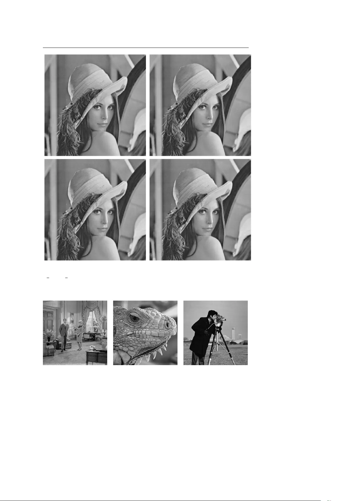
Circuits, Systems and Signal Pr ocessing manuscript No. (will be inserted by the editor) Design of a Simple Orthogonal Multiwavelet Filter by Matrix Spectral F actorization V asil Kole v · T odor Cooklev · Fritz K einert Receiv ed: date / Accepted: date Abstract W e consider the design of an orthogonal symmetric/antisymmetric multiwav elet from its matrix product filter by matrix spectral factorization (MSF). As a test problem, we construct a simple matrix product filter with desirable properties, and factor it using Bauer’ s method, which in this case can be done in closed form. The corresponding orthog- onal multiwa velet function is derived using algebraic techniques which allow symmetry to be considered. This leads to the known orthogonal multiw av elet SA1, which can also be de- riv ed directly . W e also gi ve a lifting scheme for SA1, in vestigate the influence of the number of significant digits in the calculations, and show some numerical e xperiments. Keyw ords orthogonal multiwav elets · matrix spectral factorization · Bauer’ s algorithm · Y oula and Kazanjian algorithm · lifting scheme · PLUS matrices · Alpert multiwav elet 1 Introduction and Pr oblem Formulation A digital filter bank is a collection of r filters F k ( z ) , k = 0 , . . . , r − 1, which split a discrete- time signal into r subbands. These subband signals are usually decimated by a factor of r . V asil K olev Institute of Information and Communication T echnologies Bulgarian Academy of Sciences Bl. 2 Acad. G. Bonchev St. 1113 Sofia, Bulgaria E-mail: kole v acad@abv .bg T odor Cooklev W ireless T echnology Center Purdue Univ ersity Fort W ayne, IN 46805, USA E-mail: cooklevt@pfw .edu Fritz Keinert Dept. of Mathematics Iow a State Univ ersity Ames, IA 50011, USA E-mail: keinert@iastate.edu 2 V asil K olev et al. Such a system is called a maximally decimated analysis bank . It can be used in applications such as signal, image, and video coding. F or example, a scalar wa velet system is based on a single scaling function and mother wa velet, so r = 2 [63]. In multiwav elet theory there are sev eral scaling functions and mother wavelets [18]. This provides more degrees of freedom in the design, and makes it possible to simultaneously achiev e se veral useful properties, such as symmetry , orthogonality , short support, and a higher number of v anishing moments [64]. The first multiscaling function (GHM) was constructed in 1994 by Geronimo, Hardin, and Massopust [37], based on fractal interpolation. The multiwavelet function with which the GHM multiscaling function forms a perfect reconstruction pair was constructed in a separate paper by Strang and Strela [65]. Cooklev et al. [18] in vestigated the general theory of 2 × 2 multifilter banks, and showed that real orthonormal multifilter banks and multiwav elets can be obtained from orthonormal complex-coef ficient scalar filter banks. This ensures a number of good properties, such as orthogonality , regularity , symmetry , and a lattice-structure implementation. Howe ver , the limit functions in this case tend to hav e long support. The design of multifilter banks and multiwav elets remains a significant problem. In the scalar case, spectral factorization of a half-band filter that is positiv e definite on the unit circle T in the complex plane was, in fact, the first design technique for perfect reconstruc- tion filter banks, suggested by Smith and Barnwell [59]. This pro vides motiv ation to extend Cooklev’ s original idea [17] to the multiwa velet case, where spectral factorization is more challenging. W e consider a ne w approach for obtaining an orthogonal multiwavelet which possesses symmetry/antisymmetry and re gularity , from a matrix product filter . This immediately leads to three main problems: (A) How can we obtain an appropriate matrix product filter which satisfies strong require- ments? (B) How do we perform Matrix Spectral Factorization (MSF)? (C) How do we improv e the accuracy of the computed factors? W e will consider these three problems in more detail, as well as gi ving a brief description of some basic results. Based on the previous theory and man y applications of the SA1 multiwav elet, it is useful to dev elop a lifting scheme for it. Many of the above applications can then be implemented in software or hardware to be f aster and more applicable. The paper is organized as follows. After a brief revie w of multiwavelet background, we begin by constructing a half-band product filter with good smoothness properties. W e then find a multiscaling function by using matrix spectral factorization. T o complete the de- sign by finding a multiwav elet function, we use additional algebraic techniques based on QR decomposition. The resulting multiwa velet is called SA1. It has orthogonality , symme- try/antisymmetry , piece wise smooth functions, and short support. W e then construct a lifting scheme. Finally , some experiments are sho wn with respect to this simple multiwa velet. This includes in vestigating the influence of the number of significant digits used in the calcula- tions, as well as the performance of the SA1 multiwa velet in terms of coding gain. The main nov el contributions of this paper are the follo wing: 1. W e introduce for the first time the product multifilter approach for designing a general MIMO filter bank; 2. W e obtain for the first time an orthogonal multiscaling function by using the closed form of the matrix spectral factorization algorithm of Y oula and Kazanjian [82]; Design of a Simple Orthogonal Multiwav elet 3 3. W e obtain the complementary orthogonal multiwa velet function; 4. W e construct a lifting scheme for the obtained simple orthogonal multiwa velet; 5. W e in vestigate the influence of the number of significant digits used for the coefficient √ 3, in 1D and 2D signal processing. 2 Multiwav elet Theory W e use the following notation con ventions, illustrated with the letter ’a’: a – lowercase letters refer to scalars or scalar functions; a – lowercase bold letters are vectors or v ector-v alued functions; A – uppercase letters are matrices; A – uppercase bold letters are matrix-valued functions. I and 0 are identity and zero matrices of appropriate size. A T denotes the transpose of the matrix A , and A ∗ is the complex conjugate transpose. W e are only considering real matrices in this paper . Howe ver , the variable z used in matrix polynomials lies on the unit circle T in the complex plane, so that z = z − 1 . Thus, the complex conjugate transpose of A ( z ) = ∑ k A k z k is giv en by A ( z ) ∗ = ∑ k A T k z − k . The inner product of two vector-v alued functions f ( t ) and g ( t ) in the r -dimensional Hilbert space L 2 ( R ) r of square integrable functions is gi ven by h f , g i = Z f ( t ) g ( t ) ∗ d t , which is a matrix. 2.1 Multiwa velets and the Discrete Multiwa velet T ransform Multiscaling and multiwavelet functions are vectors of r scaling functions ϕ ϕ ϕ ( t ) and r w av elet functions ψ ψ ψ ( t ) , respecti vely: ϕ ϕ ϕ ( t ) =      ϕ 0 ( t ) ϕ 1 ( t ) . . . ϕ r − 1 ( t )      , ψ ψ ψ ( t ) =      ψ 0 ( t ) ψ 1 ( t ) . . . ψ r − 1 ( t )      . They belong to L 2 ( R ) r , and satisfy the matrix dilation equations [63] ϕ ϕ ϕ ( t ) = √ 2 m ∑ k = 0 H k ϕ ϕ ϕ ( 2 t − k ) , ψ ψ ψ ( t ) = √ 2 m ∑ k = 0 G k ϕ ϕ ϕ ( 2 t − k ) . (1) 4 V asil K olev et al. Multiscaling and multiwa velet functions together are referred to as a multiwavelet . All of the functions hav e support contained in the interval [ 0 , m ] (see [79]). W e only consider orthonormal multiwav elets, where for any inte ger ` , h ϕ ϕ ϕ ( t ) , ϕ ϕ ϕ ( t − ` ) i = h ψ ψ ψ ( t ) , ψ ψ ψ ( t − ` ) i = δ 0 ` I , h ϕ ϕ ϕ ( t ) , ψ ψ ψ ( t − ` ) i = 0 . Equiv alently , the matrix coefficients H k and G k satisfy the orthonormality conditions ∑ k H k H T k + 2 ` = ∑ k G k G T k + 2 ` = δ 0 ` I , ∑ k H k G T k + 2 ` = 0 . (2) In the Discrete Multiwavelet T ransform (DMWT), the input signal s 0 , at lev el j = 0, is a sequence of r -vectors in ` 2 . For e xample, in the 2-channel case, s 0 = { s 0 k } ∞ k = − ∞ , s 0 k = " s 0 0 [ k ] s 0 1 [ k ] # , with ∑ k k s 0 k k 2 < ∞ . The DMWT of s 0 consists of computing recursi vely , for lev els j = 1 , . . . J , the approxi- mation signal s j = { s j ` } ∞ ` = − ∞ , s j ` = ∑ k H k − 2 ` s j − 1 k (3) and the detail signal d j = { d j ` } ∞ ` = − ∞ , d j ` = ∑ k G k − 2 ` s j − 1 k . (4) W e call s j ` the scaling function coefficients , and d j ` the wavelet coefficients . Because of orthogonality , the in verse can be computed iteratively in a straightforward way: s j − 1 k = ∑ ` H T k − 2 ` s j ` + ∑ ` G T k − 2 ` d j ` . (5) The matrix filter coefficients H k , G k completely characterize the multiwa velet filter bank. W e can also describe the filters and the wavelet coefficients of the signal by their symbols H ( z ) = ∑ k H k z − k , G ( z ) = ∑ k G k z − k , s j ( z ) = ∑ k s j k z k , d j ( z ) = ∑ k d j k z k . In symbol notation, one step of DMWT and in verse DMWT is described by s j ( z 2 ) = 1 2  H ( z ) s j − 1 ( z ) + H ( − z ) s j − 1 ( − z )  , d j ( z 2 ) = 1 2  G ( z ) s j − 1 ( z ) + G ( − z ) s j − 1 ( − z )  , s j − 1 ( z ) = H ( z ) ∗ s j ( z 2 ) + G ( z ) ∗ d j ( z 2 ) . (6) Decomposition and reconstruction of the DMWT for a scalar input signal s is repre- sented in fig. 1. Since s is scalar-v alued, it is necessary to vectorize it to produce s 0 . A pr e- filtering step M ( z ) is inserted at the beginning of the analysis filter bank. A corresponding postfilter N ( z ) is incorporated at the end, which is the in verse of the prefiltering step. Design of a Simple Orthogonal Multiwav elet 5 Fig. 1 T wo-channel critically sampled analysis and synthesis filter banks, with prefilter M and postfilter N ( ↓ 2 and ↑ 2 represent decimation and zero-padding). The result of ex ecuting the steps in eq. (6) is ˆ s 0 ( z ) = 1 2 [ H ( z ) ∗ H ( z ) + G ( z ) ∗ G ( z )] s 0 ( z ) + 1 2 [ H ( z ) ∗ H ( − z ) + G ( z ) ∗ G ( − z )] s 0 ( − z ) . If we want perfect reconstruction (that is, ˆ s 0 = s 0 ), we need H ( z ) ∗ H ( z ) + G ( z ) ∗ G ( z ) = 2 I , H ( z ) ∗ H ( − z ) + G ( z ) ∗ G ( − z ) = 0 . (7) The orthogonality relations (2), expressed in terms of symbols, are H ( z ) H ( z ) ∗ + H ( − z ) H ( − z ) ∗ = 2 I , G ( z ) G ( z ) ∗ + G ( − z ) G ( − z ) ∗ = 2 I , H ( z ) G ( z ) ∗ + H ( − z ) G ( − z ) ∗ = 0 (8) It is easy to show that eqs. (7) and (8) are equi valent. 2.2 Multiwa velet Denoising One of the most interesting signal processing applications is denoising . In most real ap- plications the original signals are corrupted by noise. In addition, truncation error in the computation and in other processing introduces more errors. These errors can be interpreted as additive white Gaussian noise (A WGN) e ∼ N ( 0 , σ 2 ) added to the original signal s . A denoising tec hnique is a method of remo ving the noise while retaining important features of the signal. W e consider denoising methods based on the multiwav elet transform. The wav elet transform concentrates the energy of the true signal in a few wav elet coef- ficients, while the noise energy will be scattered among all coefficients. The wav elet coef- ficients of Gaussian noise are still Gaussian. Shrinking the small coefficients tow ards zero will eliminate most of the noise, while not affecting the signal v ery much. W e use the follo wing notation. The original signal is s . This could be a one-dimensional signal s ( t ) , or an image s ( x , y ) . The noisy signal is ˜ s = s + e . The denoised signal is ˆ s . W e like wise use tildes and hats to denote the wa velet coef ficients of ˜ s , ˆ s . 6 V asil K olev et al. 2.2.1 Stochastic Sequences and Covariance Matrix Assume that the input is a noisy signal ˜ s . This is sampled and preprocessed into a vector sequence ˜ s 0 . The preprocessing is described by a linear operator M . W e also assume that postprocessing N is the in verse of preprocessing: N M = I . The discrete multiwavelet transform (DMWT) is described by a linear map Θ Θ Θ . For orthogonal multiwavelet filter banks we hav e Θ Θ Θ T Θ Θ Θ = Θ Θ Θ Θ Θ Θ T = I . It is important note the influence of the type of transform (orthonormal or biorthogo- nal) on the variance of stochastic sequences subjected to preprocessing and the DMWT . If the preprocessing M and Θ Θ Θ are orthonormal transforms, then the energy (i.e., the sum of squares of the elements) in the sequence M ˜ s is unchanged: k Θ Θ Θ M ˜ s k 2 = k M ˜ s k 2 = k ˜ s k 2 . For biorthogonal transforms, both preprocessing and matrix transformation will change the input energy . The noisy signal ˜ s is the sum ˜ s = s + e , where s is the true (deterministic) signal (noise free), and e ∼ N ( 0 , σ 2 ) is the noise, with noise power σ 2 . The goal of signal denoising is to minimize the mean square error MSE = 1 N 2 k s − ˆ s k subject to the condition that the denoised signal ˆ s is at least as smooth as s . Due to better signal representation by the multiwavelet transform, noise and signal can be separated much more easily . Multiwav elet denoising using a multiv ariate shrinkage operator effecti vely exploits the statistical information of the transformed wa velet coefficient vectors of noise, which improves the denoising perfor- mance. As a result of the decomposition and downsampling, the dependence of coefficients is reduced with increasing lev els. The multiwa velet transform Θ Θ Θ with prefilter M of the noisy signal ˜ s Θ Θ Θ M ˜ s = Θ Θ Θ M s + Θ Θ Θ M e produces the vector wa velet coefficients ˜ d j k = d j k + f j k , which are correlated with their neighbors. The scaling function coefficients s J k of the signal are fairly large, and do not need to be thresholded. W e can concentrate on the wav elet coefficients d j k of the signal, and f j k of the noise. The sequence f j = { f j k } of wavelet coefficients at le vel j of the stochastic noise has a multiv ariate normal (Gaussian) distribution f j ∼ N ( 0 , Y j ) with a cov ariance matrix cov ( f j ) = Θ Θ Θ j M j Σ M T j Θ Θ Θ T j , where Σ is the covariance matrix of the noise. The matrices Y j are r × r blocks indicating the correlation between the vector coef ficients inside each single decomposition le vel [4]. In the case of A WGN noise e ∼ N ( 0 , σ 2 e ) , cov ( f j ) = Θ Θ Θ j  σ 2 e M M T  Θ Θ Θ T j = σ 2 e Θ Θ Θ j  M M T  Θ Θ Θ T j , the cov ariance of the stochastic part depends only on the preprocessing M and the choice of multiwa velet transform Θ Θ Θ . If the preprocessing matrix satisfies M M T = I , the covariance matrix is σ 2 e I . In the general case, cov ( f j ) 6 = I is a symmetric block T oeplitz matrix. Assuming that the blocks Y j describing the correlation between the vector coefficients are known, the nonne gative scalar v alues w j k = q ( ˜ d j k ) T Y − 1 j ˜ d j k can be used for thresholding, as proposed [4]. In [28] it is shown that it is these values that should be thresholded, and the wa velet coef ficient vectors can then be adapted accordingly . Design of a Simple Orthogonal Multiwav elet 7 2.2.2 Thr esholding Rules There exist threshold and non-threshold wa velet shrinkage methods. A non-threshold wav elet shrinkage method is Besov shrinkage [22, 21]. It is known that its scale is closed under real interpolation, and it is highly adaptiv e to the local smoothness. In this paper, we consider threshold methods in more detail. This is a general wav elet denoising procedure [53, 58]. W avelet shrinkage denoising has been prov en to be nearly optimal in the mean square error (MSE) sense, and performs well in simulation studies. Thresholding methods can be grouped into two categories [61]: global thresholds and lev el-dependent thresholds. The first means that we choose a single v alue λ for the threshold, to be applied globally to all wav elet coef ficients; the second means that a possibly dif ferent threshold v alue λ j is chosen for each resolution le vel j . In what follows, we consider a global threshold λ . The threshold distinguishes between insignificant coefficients attributed to noise, and significant coefficients that encode important signal features. Signals with sparse or near sparse representation, where only a small subset of the coefficients represent all or most of the signal energy , are fit for thresholding. The noise is estimated by a properly chosen threshold after the multiwa velet transform. Filtering of additi ve Gaussian noise (zero mean and standard deviation σ ) via the thresh- olding of wa velet coefficients was pioneered by Donoho [24]. A wav elet coefficient ˜ d j k is compared with a universal threshold λ . If the coefficient has a magnitude smaller than the threshold, it is considered to be noise, and is set to zero. Otherwise, is kept or modified, depending on the thresholding rule. In this paper hard and soft thresholding methods will be considered. The v ector wav elet coefficients thresholded by the soft thresholding rule are ˆ d j k =      ˜ d j k w j k − λ w j k , w j k ≥ λ , 0 , w j k < λ . For the hard thresholding rule, the y are ˆ d j k = ( ˜ d j k , w j k ≥ λ , 0 , w j k < λ . Another method, semisoft thresholding, has been proposed [50, 83], but so far only for the scalar wa velet setting. The vector wav elet coefficients d j k could be thresholded using either the hard or soft thresholding rules. These thresholding rules hav e strong connections with model selection in the traditional linear models. The trick of thresholding is to include these irregularities while excluding the noise [27]. In general, in terms of visual quality , the noise reduction ef fect of soft thresholding is the best, follo wed by the impro ved semisoft shrinkage method; the hard thresholding method is the worst. Hard shrinkage produces smaller bias but larger variance than soft shrinkage, and em- pirically performs better than soft shrinkage minimax estimation [10]. It better retains local characteristics of the image edges [24, 66], and is suitable for denoising of noise with sudden changes. Howe ver , it introduces sudden jumps in the multiwav elet domain that in turn lead to oscillations in the reconstructed images. These oscillations are very close to the Gibbs 8 V asil K olev et al. phenomenon (see fig. 3 in [31]) and are called pseudo-Gibbs phenomena . They affect the visual quality of the denoising image, and manifest themselves as annoying artifacts in the denoised image (see Fig. 2(a)). The soft thresholding method smoothes the jumps in the wav elet domain by shrinking also the coefficients near the jumps. The denoised signals end up relativ ely smooth, and the pseudo-Gibbs phenomenon is reduced to some extent. Better results are expected in the future by using the multiple description approach for the multiwa velet transformation sho wn in [77]. 2.2.3 Universal Thr eshold The threshold value λ is a very important parameter , which directly influences the perfor- mance of wa velet denoising. It can be determined by estimating the v ariance of the noise in images, but thise v alue is often unknown in applications. Using a uni versal threshold v alue, instead of a dif ferent threshold at each le vel, is attrac- tiv ely simple, but is strictly suitable only when thresholding A WGN wavelet coef ficients of variance σ 2 and mean zero. The basic idea is that if the signal component is in fact zero, then with high probability the combination of (zero) signal plus noise should not exceed the threshold le vel λ = σ e √ 2 log N , where N is the length of the signal. The uni versal threshold λ [24, 27] pays attention to smoothness rather than to minimizing the mean square error (MSE). This threshold is the asymptotic infimum, the asymptotic optimal threshold [25], and comes close to the minimax threshold, i.e. the threshold that minimizes the worst case MSE [26]. The tri vial extension of the univ ersal threshold to multiple wavelet coefficients is to use the threshold abov e applied to each coefficient element. In the numerical examples in this paper, we are using the follo wing Algorithm 1. It im- plements the algorithm described in the text, adapted to two-dimensional signals (images). Algorithm 1: Image Denoising Algorithm Based on Multiwav elet T ransform Step 1 Apply the pre-filtering M to all rows, then all columns (of previously row pre- filtered pixels) of the noisy image ˜ s Step 2 Apply the 2D forward multiwa velet transform row by row and column by col- umn, up to lev el J Step 3 Choose the uni versal threshold λ and apply a ( har d or soft ) thresholding proce- dure to the resulting multiwav elet coef ficients ˜ d j k to obtain the denoised wav elet coefficients ˆ d j k Step 4 Apply the 2D backward multiwa velet transform up to le vel J Step 5 Apply the post-filtering N , producing a denoised image ˆ s 2.3 The Multiwa velet SA1 In this section, we describe a simple multiwav elet that will be used in the remainder of this paper to illustrate our approach. W e are interested in supercompact multiwavelets, that is, multiwa velets with support in [ 0 , 1 ] . Such functions have man y advantages: – Application to functions defined on a finite interval does not require any special treat- ment at the boundaries of the interval [7]; – Interpolation with non-equally spaced data is possible [20, 41]; – Application to functions that are only piecewise continuous (internal boundaries) can be efficiently implemented [7, 48, 51]; Design of a Simple Orthogonal Multiwav elet 9 (a) (b) Fig. 2 The scaling and w avelet functions of SA1; (a) the multiscaling function ϕ ϕ ϕ ( t ) = [ ϕ 0 ( t ) , ϕ 1 ( t )] T ; (b) the multiwav elet function ψ ψ ψ ( t ) = [ ψ 0 ( t ) , ψ 1 ( t )] T . – It is easy to construct a nodal basis with (spectral) finite elements [5, 55]; – Polynomials are reconstructed exactly [7]; – Discontinuities in the signal are easy to detect [80], and the size of jumps at element boundaries can be measured, in 1D [74] and 2D [75]; – Construction of the operation matrices in numerical methods is simple [1, 23]; – Supercompact multiwav elets with the v anishing moment property are suitable for adap- tiv e solvers of PDEs subject to boundary conditions, as well as for solving of a wide class of integro-dif ferential operators having sparse representation in these bases. Alpert [2] already observed that a multiscaling function whose entries form a basis of polynomials of degree p on [ 0 , 1 ] will always be refinable. For p = 0, this leads to the Haar wavelet. For p = 1, we can take φ 0 = Haar wavelet, and φ 1 = any non-constant linear polynomial. If we want φ 1 to be orthogonal to φ 0 and normalized, we find that for t ∈ [ 0 , 1 ] , φ 0 ( t ) = 1 , φ 1 ( t ) = √ 3 ( 1 − 2 t ) . This choice is unique, up to sign. The two components of ϕ ϕ ϕ are shown in fig. 2(a). The refinement coefficients are easy to deri ve with elementary algebra: we find H 0 = √ 2 4  2 0 √ 3 1  , H 1 = √ 2 4  2 0 − √ 3 1  . (9) The completion with a corresponding multiwav elet function is not unique, b ut by impos- ing orthogonality and symmetry constraints we find an essentially unique completion with recursion coefficients G 0 = √ 2 4  0 2 − 1 √ 3  , G 1 = √ 2 4  0 − 2 1 √ 3  . (10) Details are giv en in section 4.2. The corresponding functions are described by ψ 0 ( t ) = ( √ 3 ( 1 − 4 t ) t ∈ [ 0 , 1 2 ] , √ 3 ( 4 t − 3 ) t ∈ [ 1 2 , 1 ] , ψ 1 ( t ) = ( ( 1 − 6 t ) t ∈ [ 0 , 1 2 ] , ( 5 − 6 t ) t ∈ [ 1 2 , 1 ] . They are sho wn in fig. 2(b). W e call this multiwav elet SA1. 10 V asil K olev et al. 3 Matrix Product Filters 3.1 Theory of Matrix Product Filters Giv en a matrix filter H ( z ) = m ∑ k = 0 H k z − k , its matrix pr oduct filter P ( z ) is defined as P ( z ) = H ( z ) H ( z ) ∗ = m ∑ k = − m P k z k , where P k = H 0 H T k + · · · + H m − k − 1 H T m − 1 + H m − k H T m . In particular for k = 0, P 0 = H 0 H T 0 + · · · + H m − 1 H T m − 1 + H m H T m . The Laurent polynomial matrix P ( z ) ∈ C r × r [ z , z − 1 ] is a discrete-time para-Hermitian matrix. Here C r × r [ z , z − 1 ] is the ring of r × r matrices whose elements are polynomials in z , z − 1 with complex coefficients [9]. By the first equation in (8), it is a half-band filter [18], which means it satisfies the equation P ( z ) + P ( − z ) = 2 I . (11) This implies P 0 = I , P 2 k = 0 for k 6 = 0 . W e can similarly define the half-band filter Q ( z ) = G ( z ) G ( z ) ∗ . Every orthogonal multiscaling filter H ( z ) is a spectral factor of some half-band multifil- ter . W e use this fact as the starting point for constructing multiwa velets: Construct a suitable P ( z ) first, and factor it to obtain H ( z ) . In the scalar case, spectral f actorization is one of the main design techniques [8, 63]. F or r > 1, matrix spectral factorization is required, which is more challenging. 3.2 Matrix Spectral Factorization A critical component in classical spectral decomposition is the F ej ´ er-Riesz theor em for pos- itiv e definite functions [13]. Fej ´ er [34] was the first to note the importance of the class of trigonometric polynomials that assume only non-ne gati ve real values; the theorem w as con- sidered and prov ed by Riesz [52]. The Fej ´ er-Riesz theorem in one dimension considers a trigonometric polynomial ex- pressed in the form ν ( z ) = N ∑ k = − N ν k z k . Design of a Simple Orthogonal Multiwav elet 11 When ν ( z ) is real for all z ∈ T , the coefficients satisfy ν k = ν − k for all k . The theorem states that if ν ( z ) ≥ 0 for all z ∈ T , such a ν ( z ) is expressible in the form ν ( z ) = p ( z ) p ( z ) ∗ for some polynomial p ( z ) = ∑ N k = 0 p k z k . As noted in [32], a spectral factor p ( z ) is unique up to a constant right unitary multiplier U ( z ) , i. e. p new ( z ) = p ( z ) U ( z ) . The Fej ´ er-Riesz theorem does not extend to factorization of multiv ariate trigonometric polynomials (see [29] for some counterexamples). Rele vant ke y theorems are [54, Theorem 3.2] in the 1D case, [29, Theorem 6.2] for the 2D case, with examples and necessary and sufficient conditions in [38], and [54, Theorem 3.1] for arbitrary dimensions. Howe ver , the theorem can be e xtended to the case of uni variate polynomials with matrix coefficients. This is Matrix Spectr al F actorization (MSF) (see [73, 12, 33, 82]). The MSF problem plays a crucial role in the solution of various applied problems for MIMO systems in communications and control engineering [9, 45, 78, 81]. 3.3 Bauer’ s Method A well-known method for MSF is Bauer’ s method [6]. This method has been successfully applied in [14, 30, 35, 39]. Details of the algorithm are gi ven in section 4.1 belo w . Bauer’ s method, in the implementation of Y oula and Kazanjian [47, 46, 49, 82], has the advantage over other approaches that it can handle zeros of the determinant of P ( z ) on T . Unfortunately , the presence of these zeros af fects the accurac y and speed of con vergence. In its original form, the method only gi ves us a low precision spectral factor , and con vergence is very slo w . The approaches in [33] for finding precision spectral factors can be used instead. For instance, the Janashia-Lagvilav a MSF method for the orthogonal SA4 multiwa velet consid- ered in [33] is exact. In this paper, we achiev e an exact MSF leading to a simple orthogonal multiwavelet by the closed form of Bauer’ s method for short product filters. This is possible for some types of short support multiwa velets, especially the supercompact multiwa velets [7]. 3.4 A Simple Matrix Product Filter The simplest non-scalar example is for r = 2, m = 1. In this case, P ∈ C 2 × 2 [ z , z − 1 ] has the form P ( z ) = P T 1 z − 1 + P 0 + P 1 z . (12) From the half-band condition (11) we see that P 0 is the identity matrix. The smoothness of the multiscaling and multiwav elet functions is improved if the de- terminant of the product filter has a higher-order zero at z = − 1 (see [72]). Therefore, we choose det ( P ( z )) =  1 + z − 1 2  k q ( z ) , (13) where q ( z ) is a linear phase polynomial in z , and k is necessarily ev en. 12 V asil K olev et al. The simplest case corresponds to k = 4 and q ( z ) = z 2 , where det ( P ( z )) =  1 + z − 1 2  4 z 2 = 1 16  z − 2 + 4 z − 1 + 6 + 4 z + z 2  . Setting P 1 =  a b c d  , we find the equations ad − bc = 1 / 16 , a + d = 4 / 16 , 1 − b 2 − c 2 + 2 ad = 6 / 16 . These equations have precisely four solutions: either a = 1 / 2, d = − 1 / 4 or a = − 1 / 4, d = 1 / 2, and in both cases we can choose b = − c = ± √ 3 / 4. Ho wev er , these are all es- sentially equiv alent. The different choices just correspond to interchanging φ 0 and φ 1 , or changing the sign of one of the functions. W e choose a = 1 2 , b = − √ 3 4 , c = √ 3 4 , d = − 1 4 . The resulting product filter has coefficient P 1 = 1 4  2 − √ 3 √ 3 − 1  . (14) 4 Design of Orthogonal Multiwav elet Filter 4.1 Finding H ( z ) For simplicity , we only describe the details of Bauer’ s method for the case m = 1 considered in this paper . The equation P ( z ) = H ( z ) H ( z ) ∗ is equiv alent to the fact that the infinite block tridiagonal matrix P =       . . . . . . . . . P T 1 P 0 P 1 P T 1 P 0 P 1 . . . . . . . . .       can be factored as P = H H T , where H is the infinite block bidiagonal matrix H =       . . . . . . H 1 H 0 H 1 H 0 . . . . . .       For a chosen integer n , we truncate P to the matrix P n of size ( n + 1 ) × ( n + 1 ) , and do a Cholesky factorization P n = H n H T n . The last row of H n will be H ( n ) 1 , H ( n ) 0 . Design of a Simple Orthogonal Multiwav elet 13 The YK theory says that H ( n ) 0 → H 0 as n → ∞ , and likewise for H 1 . The computation can be streamlined, by defining X ( k ) = H ( k ) 0 h H ( k ) 0 i T , k = 0 , 1 , . . . . The Cholesky factorization algorithm is equi valent to X ( 0 ) = P 0 , X ( k + 1 ) = P 0 − P T 1 h X ( k ) i − 1 P 1 . (15) The limit matrix X satisfies X = P 0 − P T 1 X − 1 P 1 . (16) W e can use fixed point iteration based on (15) to av oid forming the large matrix P n . Once X has been found to sufficient accuracy , we can find H 0 as the Cholesky factor of X , and H 1 = P T 1 H − T 0 . Even better, in the simple case considered in this paper , the Symbolic Math toolbox in Matlab is able to solve equation (16) in closed form. On a MacBook Air with 2.2GHz Intel i7 processor, using Matlab 9.1, the computational time is under 0.8 sec. W e get the exact matrix spectral factor with coef ficients H 0 = √ 2 4  2 0 √ 3 1  , H 1 = √ 2 4  2 0 − √ 3 1  . (17) This is precisely the multiscaling function of SA1, introduced in section 2.3. The spectral factor obtained by our closed form of Bauers method is precise. This mul- tiscaling function can also be obtained from the 4x4 T ype-II DCT matrix [36] and by using the Janashia-Lagvila va method [33] in e xact form. It can also be obtained approximately by the Janashia-Lagvilav a matrix spectral factorization method (see procedure 2 in [42]), with an error in the spectral factors of about 10 − 8 . 4.2 Finding G ( z ) The orthogonality conditions (2) in the case m = 1 simply state that the matrix  H 0 H 1 G 0 G 1  must be orthogonal. W e can find an initial orthogonal completion [ ˆ G 0 , ˆ G 1 ] from a QR- decomposition of [ H 0 , H 1 ] T . Matlab returns [ ˆ G 0 , ˆ G 1 ] = √ 2 4  1 − √ 3 − 1 − √ 3 0 2 0 − 2  . Any other orthogonal completion has to be of the form [ G 0 , G 1 ] = U · [ ˆ G 0 , ˆ G 1 ] for orthogonal U . W e want to choose a U that introduces symmetry . 14 V asil K olev et al. A function f ( t ) is symmetric about a point a if f ( a + t ) = f ( a − t ) . It is antisymmetric about a if f ( a + t ) = − f ( a − t ) . For multiscaling and multiwa velet functions, we only con- sider the simplest case, where each component ϕ i or ψ i is symmetric or antisymmetric about the midpoint m / 2. Thus, ϕ ϕ ϕ ( m 2 + t ) = S · ϕ ϕ ϕ ( m 2 − t ) , (18) where S is a diagonal matrix with entries 1 (symmetry) or ( − 1 ) (antisymmetry). Like wise, ψ ψ ψ ( m 2 + t ) = T · ψ ψ ψ ( m 2 − t ) . It is not hard to show that ϕ ϕ ϕ , ψ ψ ψ have the symmetry gi ven by S , T if and only if H k = SH m − k S , G k = T G m − k S , k = 0 , . . . , m . (19) In our example, we observ e that the original factors (17) already satisfy H 1 = SH 0 S for S = diag ( 1 , − 1 ) . That is, component ϕ 0 is symmetric, ϕ 1 is antisymmetric. The symmetry conditions (19) for G are U ˆ G 0 = T U ˆ G 1 S , U ˆ G 1 = T U ˆ G 0 S , which leads to U = T U ˆ G 1 S ˆ G − 1 0 = − T U S . It is easy to check that T = ± I is not possible, so T = ± S . W e choose T = S , which means that we want ψ 0 to be symmetric, ψ 1 antisymmetric. Any U of the form U =  0 ± 1 ± 1 0  is then suitable. The choice of signs corresponds to changing the sign of ψ 0 and/or ψ 1 . Using U =  0 1 − 1 0  leads to the same G 0 , G 1 as in (10). Choosing T = − S would interchange ψ 0 and ψ 1 , and giv e us U =  ± 1 0 0 ± 1  , which again corresponds to sign changes. Design of a Simple Orthogonal Multiwav elet 15 (a) (b) Fig. 3 One lifting step; (a) analysis part; (b) synthesis part. 5 Efficient Implementation W e giv e here a brief overvie w of the lifting scheme (LS) and some rounding operations. Lifting steps are an efficient implementation of filtering operations (see fig. 3(a)). One lifting step for a filter bank consists of an operation Split , a prediction P , and an update U . One of the great adv antages of LS is that it decomposes a multiw av elet filter into simple in vertible steps [11, 67]. The inv erse LS can be obtained from the forward LS by reversing the order of the operations, in verting the signs in the lifting steps, and replacing the Split by a Mer ge step (see fig. 3(b)). If a floor (or r ound or ceiling ) operator is placed in each lifting step, the filter banks can now map integers to integers with perfect reconstruction, regardless of whether the lifting step has integer coef ficients or not. Moreov er , if the factors are chosen to be dyadic, multiplication can be implemented by addition and binary bit shift. If the integer mantissa k in a lifting step with coef ficient c = k · 2 − b 0 is written in binary notation as k = ∑ k i 2 i , k i = 0 or 1 , then the multiplication of a number x by c can be implemented by adding copies of x , left- shifted by i , for each k i 6 = 0, and a final right-shift by b 0 bits. This approach leads to an implementation with solely binary shifts, prev enting bit-depth expansion in intermediate results. With all scaling factors set to unity , multiplierless filter banks can be easily constructed using this method. If the scaling factors are powers of two, we can still retain the multiplierless feature on filter banks. The lifting scheme can be done in place: we nev er need samples other than the output of the pre vious lifting step, and therefore we can replace the old stream by the new stream at ev ery summation point. 5.1 The Lifting Scheme Based on matrix f actorization theory [40], a nonsingular matrix can be factored into a prod- uct of at most three triangular elementary PLUS reversible matrices [56, 76, 44]. If the di- agonal elements of the matrices are ones, a rev ersible integer-to-integer transform can be realized by LS. In order to speed up the implementation, it is necessary to optimize the elementary trian- gular factorization by either minimizing the number of factorized matrices or the computa- tional complexity of each step. The factorization is not unique, and there are other different factorizations that af fect the error between the dyadic approximation transform and the orig- inal transform. 16 V asil K olev et al. (a) (b) Fig. 4 The PLUS matrices implementation of H ; (a) forw ard; (b) backward. For input vector x = [ x 0 , x 1 , x 2 , x 3 ] T and output vector y = [ y 0 , y 1 , y 2 , y 3 ] T , the lifting implementation of the forward DMWT (6) is y = H x = ( PL U ) x =     1 0 0 0 0 0 0 1 0 1 0 0 0 0 1 0         1 0 0 0 0 1 0 0 − 1 2 √ 3 2 1 0 √ 3 2 1 2 − √ 3 1         1 0 1 0 0 1 0 − 1 0 0 1 √ 3 0 0 0 4         x 0 x 1 x 2 x 3     . (20) This leads to the synthesis implementation H − 1 = 1 2 U − 1 L − 1 P T . (21) W e include the factor of ( 1 / 2 ) with the reconstruction instead of the decomposition (see (6)). In our implementation, we write the L and U matrices as products of elementary trian- gular and/or diagonal rev ersible matrices (see [62], page 34), for faster ev aluation. L =     1 0 0 0 0 1 0 0 − 1 / 2 √ 3 / 2 1 0 0 0 0 1         1 0 0 0 0 1 0 0 0 0 1 0 √ 3 / 2 1 / 2 − √ 3 1     , U =     1 0 0 0 0 1 0 0 0 0 1 0 0 0 0 4         1 0 0 0 0 1 0 − 1 0 0 1 √ 3 0 0 0 1         1 0 1 0 0 1 0 0 0 0 1 0 0 0 0 1     The implementation of the lifting scheme is shown in fig. 4. 5.2 Multiplierless architecture of the coefficient √ 3 For the transform to be reversible, it must be able to exactly reconstruct the input from the output. Low computational complexity is another desirable property . In order to av oid floating-point multiplications, we approximate v alues of the lifting matrices by dyadic num- bers. The lifting scheme described in subsection 5.1 uses only a single non-dyadic number , which is √ 3. W e want to approximate this coefficient by a number of the form k · 2 − b 0 with Design of a Simple Orthogonal Multiwav elet 17 (a) (b) (c) (d) Fig. 5 Floating-point arithmetic (solid line) in comparison with fixed point arithmetic (dash-dot line) of the impulse responses of the SA1 orthogonal multiwavelet, with 2-bit dyadic approximation of the coefficient √ 3 (that is, √ 3 ≈ 3 / 2); (a) φ 0 ; (b) φ 1 ; (c) ψ 0 ; (d) ψ 1 . integer k . Since √ 3 is between 1 and 2, this corresponds to an approximation with ( b 0 + 1 ) bits. For example, for b 0 = 5, √ 3 is approximated by the 6-bit number 55 · 2 − 5 = 1 . 71875, with an error of approximately 1 . 73205 − 1 . 71875 = 0 . 0133. The dyadic approximations of the coef ficient √ 3 and its quantization errors are sho wn in table 1. The table also sho ws the number of adders required to implement the multiplierless structure. W e illustrate the ef fect of quantization for b 0 = 1 in more detail. This is the case of 2-bit approximation, with √ 3 ≈ 3 / 2. The true recursion coef ficients of SA1 are given in eqs. (9) and (10). The actual recursion coefficients used in the 2-bit approximation are ˜ H 0 = √ 2 4  2 0 1 . 5 1  , ˜ H 1 = √ 2 4  2 0 − 1 . 5 1  , ˜ G 0 = √ 2 4  0 2 − 1 1 . 5  , ˜ G 1 = √ 2 4  0 − 2 1 1 . 5  . (22) 18 V asil K olev et al. T able 1 Different quantizations of the non-trivial coefficient √ 3 ≈ k · 2 − b 0 , with k an integer represented by ( b 0 + 1 ) bits. For example, for b 0 = 5, the approximation is √ 3 ≈ 55 · 2 − 5 = 1 . 71875, with an error of approximately 1 . 73205 − 1 . 71875 = 0 . 0133. The table also shows the number of adders needed to realize the multiplierless structure. Entries in bold mark the places where increasing the number of bits does not change the approximation. b 0 = binary exponent mantissa adders quantization error 1 3 1 0 . 232050807568877 2 7 2 − 0 . 017949192431123 3 14 2 − − −− 4 28 2 − − −− 5 55 2 0 . 013300807568877 6 111 2 − 0 . 002324192431123 7 222 2 − − −− 8 443 3 0 . 001582057568877 9 887 3 − 0 . 000371067431123 10 1774 3 − − −− 11 3547 4 0 . 000117213818877 12 7094 4 − − −− 13 14189 4 − 0 . 000004856493623 14 28378 4 − − −− These approximate matrix coefficients (22) satisfy ˜ H ( z ) ˜ H ( z ) ∗ + ˜ H ( − z ) ˜ H ( − z ) ∗ =  2 0 0 13 8  , ˜ G ( z ) ˜ G ( z ) ∗ + ˜ G ( − z ) ˜ G ( − z ) ∗ =  2 0 0 13 8  , ˜ H ( z ) ˜ G ( z ) ∗ + ˜ H ( − z ) ˜ G ( − z ) ∗ = 0 instead of the true orthogonality conditions (8). This leads to a decrease of CG to 2 . 01 dB and non-perfect reconstruction, which is undesirable in many mathematical and engineering applications. The ef fect of rounding can also be illustrated by its ef fect on the multiscaling and multi- wa velet functions. It is easy to verify that the functions which satisfy the rounded recursion relations corresponding to (1) are ˜ φ 0 ( t ) = 1 , ˜ φ 1 ( t ) = 3 2 ( 1 − 2 t ) and ˜ ψ 0 ( t ) = ( 3 2 ( 1 − 4 t ) t ∈ [ 0 , 1 2 ] , 3 2 ( 4 t − 3 ) t ∈ [ 1 2 , 1 ] , ˜ ψ 1 ( t ) = ( 5 8 − 9 2 t t ∈ [ 0 , 1 2 ] , 31 8 − 9 2 t t ∈ [ 1 2 , 1 ] . This is illustrated in fig. 5. The biggest differences are at the end points, which are marked by squares in the figure. Obviously , the dyadic approximation strongly influences the sloped parts in time do- main, which leads to smaller magnitudes for the scaling function ˜ φ 1 , as well as both wav elet functions ˜ ψ 0 and ˜ ψ 1 . Design of a Simple Orthogonal Multiwav elet 19 T able 2 Comparison of CG, symmetric/antisymmetric properties (SA), Sobolev regularity (S) and autocor- relation matrix R x of AR(1) and ρ = 0 . 95. Multiwav elet CG S SA Length Biorthogonal (dual to Hermitian cubic spline) ( ’bih32s’ ) [3] 1.01 2.5 yes 3/5 Biorthogonal Hermitian cubic spline ( ’bih34n’ ) [66] 1.51 2.5 yes 3/5 Integer Haar [15] 1.83 0.5 yes 2 CL [16] 2.06 1.06 yes 3 SA1 2.13 0.5 yes 2 SA4 [57] 3.73 0.99 yes 4 GHM [37] 4.41 1.5 yes 4 6 Perf ormance Analysis 6.1 Comparativ e Analysis The objective of this section is to ev aluate numerically the performance of the SA1 mul- tiwa velet, and compare it to some well-known orthogonal and biorthogonal multiwavelets, with the criteria being coding gain (CG) [60, 70], Sobole v smoothness (S) [43], symmetry/anti- symmetry (SA), and length. The CG for orthogonal transforms is a good indication of the performance in signal processing. It is the ratio of arithmetic and geometric means of chan- nel variances CG = 1 r ∑ r i = 1 σ 2 i  ∏ r i = 1 σ 2 i  1 / r . (23) Coding gain is one of the most important factors to be considered in man y applications. A transform with higher coding gain compacts more ener gy into a smaller number of coeffi- cients. A comparison of CGs is gi ven in table 2. Sobole v re gularity , symmetry/antisymmetry properties and the length of the given multiwav elets are also included. The CG is com- puted using a first order Markov model AR(1) with intersample autocorrelation coefficient ρ = 0 . 95 [71]. Obviously , despite the short length (only two matrix coef ficients) of the sim- ple multiwav elet SA1, its CG is better than that of most of the orthogonal and biorthogonal multiwa velets. 6.2 Pre- and Postfilters In the case of a scalar-v alued input signal to the multiple-input multiple-output (MIMO) filter bank it is necessary to vectorize the input. In other words, a pre-processing step (called pr efiltering ) must be inserted at the beginning of the analysis multifilter; in a symmetric way , a postfilter must be incorporated at the end of the synthesis filter bank. In practical applications, a popular choice is based on the Haar transforms [19, 68]. Haar pre- and postfilters ha ve the adv antage of simultaneously possessing symmetry and orthogonality , and no multiplication is needed if one ignores the scaling f actor . The prefilters should be as short as possible to preserve the time localization of the wa velet decomposition. The choice of prefilter is often critical for the results, and should be made depending on the application at hand and the type of signal to be processed. The postfilter N ( z ) that accompanies the prefilter M ( z ) must satisfy N ( z ) M ( z ) = I . The matrix coefficients of the pre- and postfilters we used are sho wn in table 3. 20 V asil K olev et al. T able 3 The matrix coefficients of the pre- and postfilters for GHM, CL, and SA1 orthogonal multiw avelets M ( z ) N ( z ) GHM 1 8 √ 2  3 10 0 0  +  3 0 8 √ 2 0  z − 1  1 10  0 10 0 − 3  z +  0 0 8 √ 2 − 3  CL  1 / 4 1 / 4 1 / ( 1 + √ 7 ) − 1 / ( 1 + √ 7 )   2 ( 1 + √ 7 ) / 2 2 − ( 1 + √ 7 ) / 2  SA1 1 √ 2  1 1 1 − 1  1 √ 2  1 1 1 − 1  6.3 Dyadic approximation of a 1D signal As explained in section 5.2, the customer often prefers a simple dyadic approximation of the coefficients. For a chosen b 0 and J , we let ˆ s 1 , J be the signal obtained by decomposing and reconstructing through J lev els, using ( b 0 + 1 ) bits of accuracy . W e define the quantization err or by the norm k ε 1 , J k ∞ = max i | ε 1 , J ( i ) | , where ε 1 , J ( i ) = s ( i ) − ˆ s 1 , J ( i ) . W e mainly will consider balanced and non-balanced multiwavelet decomposition and synthesis without processing with a 2-bit approximation of the coefficient √ 3, i. e. b 0 = 1, √ 3 ≈ 3 / 2. The non-balanced DMWT con verts the scalar input signal into a vector input signal by simple partitioning. The balanced D WMT uses a preprocessing and postprocessing step. Results of using the SA1 balanced filter bank with the Haar pre- and postfilters giv en in table 3, for the ’Piece-Regular’ signal with 2 10 samples, through 2 and 6 decomposition lev els, with their these quantization errors are sho wn in fig. 6(a), (b). Obviously , increasing the decomposition lev el leads to an increase in quantization error . It is important to note that the reconstructed signal follows the input signal, except at spikes where the local maxima of the quantization errors are achiev ed. The best results are obtained at small decomposition levels, between 1 and 4, as shown in fig. 6(a). Higher decomposition le vels lead to an increase of the quantization errors o ver the input signal; see fig. 6(b). In contrast to the balanced SA1 multiwa velet, the quantization errors of the non-balanced SA1 multiw avelet are very different, and poor . The reconstructed signal oscillates around the analyzing signal, and the quantization errors are bigger than the balanced version, even at low le vels, as shown in fig. 7(a). Detailed information about the minimal and maximal quantization errors, measured by the norm k ε 1 , J k ∞ for the test signal ’Piece-Regular’ (see fig. 6), and the additional test signal ’Piece-Polynomial’ (see fig. 8) with 2 9 to 2 13 samples are tabulated in tables 4 and 5. The minimal quantization errors are at the first decomposition le vel for all lengths of both test signals, while the maximum errors depend on the test signal. There are only minor differences in the minimal quantization errors for the ’Piece-Regular’ signal for all signal lengths, which means that the minimal quantization error is almost independent of the length of this signal. Design of a Simple Orthogonal Multiwav elet 21 (a) (b) Fig. 6 Influence of the number of decomposition levels J of the 2-bit dyadic approximations for the co- efficient √ 3 ( i. e. √ 3 ≈ 3 / 2) of the balanced SA1 multiwavelet analysis and synthesis filter bank with- out processing, for the ’Piece-Regular’ signal with i = 2 10 samples through (a) J = 2 levels with k ε 1 , 2 k ∞ = 0 . 1317; (b) J = 6 levels with k ε 1 , 6 k ∞ = 0 . 2535. In both (a) and (b), the top image shows the original signal s and reconstruction ˆ s 1 , J ; the bottom image shows the error ε 1 , J . (a) (b) Fig. 7 Influence of the number of decomposition levels J of the 2-bit dyadic approximations for the co- efficient √ 3 ( i. e. √ 3 ≈ 3 / 2) of the non-balanced SA1 multiwavelet analysis and synthesis filter bank without processing, for the ’Piece-Regular’ signal with i = 2 10 samples through (a) J = 2 levels with k ε 1 , 2 k ∞ = 0 . 2148; (b) J = 8 levels with k ε 1 , 8 k ∞ = 0 . 3239. In both (a) and (b), the top image shows the original signal s and reconstruction ˆ s 1 , J ; the bottom image shows the error ε 1 , J . 22 V asil K olev et al. T able 4 Dependence of the norm k ε 1 , J k ∞ on the number of decomposition lev els J for the balanced SA1 multiwav elet without processing. The 2-bit dyadic approximation of the coefficient √ 3 (i. e. √ 3 ≈ 3 / 2) is applied to the ’Piece-Regular’ signal. Decomp. T est signal length lev els 2 9 samples 2 10 samples 2 11 samples 2 12 samples 2 13 samples 1 0.06084 0.06149 0.06695 0.06646 0.06103 2 0.12786 0.13167 0.12747 0.14190 0.10010 3 0.18903 0.13848 0.13056 0.14656 0.13211 4 0.23077 0.18432 0.18191 0.17597 0.13931 5 0.26208 0.21887 0.16843 0.20945 0.14795 6 0.29277 0.25346 0.21485 0.17841 0.18582 7 0.26932 0.28641 0.26010 0.22375 0.17793 8 0.26101 0.28482 0.26315 0.22557 9 0.29099 0.29428 0.26304 10 0.30911 0.29569 11 0.28781 T able 5 Dependence of the norm k ε 1 , J k ∞ on the number of decomposition lev els J for the balanced SA1 multiwav elet without processing. The 2-bit dyadic approximation of the coefficient √ 3 (i. e. √ 3 ≈ 3 / 2) is applied to the ’Piece-Polynomial’ signal. Decomp. T est signal length lev els 2 9 samples 2 10 samples 2 11 samples 2 12 samples 2 13 samples 1 0.05834 0.13124 0.13118 0.13073 0.05770 2 0.13597 0.25323 0.27918 0.27996 0.13145 3 0.25061 0.26580 0.38819 0.29392 0.26348 4 0.25272 0.37841 0.32504 0.39067 0.28238 5 0.31074 0.32303 0.37016 0.31828 0.39400 6 0.26599 0.30530 0.33977 0.38265 0.33192 7 0.26648 0.36935 0.36768 0.33015 0.37298 8 0.36903 0.36846 0.35761 0.34802 9 0.36837 0.36052 0.37613 10 0.36055 0.37174 11 0.37168 0 5 0 0 1 0 0 0 0 0 . 5 1 0 500 1000 -0.5 0 0.5 1 Fig. 8 Additional test signal ’Piece-Polynomial’ Design of a Simple Orthogonal Multiwav elet 23 The minimal quantization errors for the ’Piece-Polynomial’ signal for signal lengths 2 10 to 2 12 samples are nearly equal, but for 2 9 and 2 13 samples decrease by more than a factor of 2. The maximum quantization errors for the ’Piece-Regular’ signal are at the first and next to last levels and are nearly equal, and for the ’Piece-Polynomial’ signal at decom- position lev els 4 or 5. Note that the minimal quantization errors are in the range [ 0 . 01 , 0 . 05 ] , but the maximal quantization errors are in the range [ 0 . 3 , 0 . 4 ] , which leads to visible artifacts in signal and image processing. 6.4 Dyadic approximations for 2D signals In this subsection, we consider the influence of 2-bit ( √ 3 ≈ 3 / 2) and 3-bit ( √ 3 ≈ 7 / 4) dyadic approximation applied to analysis and reconstruction filter bank without processing, in the context of the balanced and non-balanced SA1 multiwav elet. W e will consider the gray scale image ’Lena’ of size 256 × 256 pixels. The first example illustrates the effect of the 2-bit dyadic approximation of the coeffi- cient √ 3 (i. e. √ 3 ≈ 3 / 2). As we can see see from fig. 9(a), image processing with the SA1 non-balanced multiwav elet filter bank leads a grid artifact over the whole image. Further - more, with more than one decomposition le vel the obtained images are usually unusable. It is also important to note that after more than J = 4 decomposition levels, the multiwav elet processing with the balanced filter bank sho ws visible square edge artif acts, e ven though the PSNR can be high. This is shown in fig. 9(b). The second e xample illustrates a comparison of 3-bit dyadic approximation of the coef- ficient √ 3 (i.e. √ 3 ≈ 7 / 4). It is obvious from fig. 10(a) and (b) that the SA1 multiwav elet processing with both non-balanced and balanced filter bank leads to high quality images. Therefore, in some applications we prefer 3-bit dyadic approximation of the coef ficient √ 3, which does not lead to undesired image artifacts. 6.5 Image Denoising In order to suppress the noise coefficients, the noisy image is first transformed to the mul- tiwa velet domain, and then soft or hard vector thresholding is applied at various resolution lev els. This is described in more detail in subsection 2.2. W e apply image denoising to the test images shown in fig. 11 and fig. 12, using the lifting scheme (eqs. (20) and (21)) and the multiwavelet decomposition in [69], for three multiwa velets GHM, CL, and SA1. The images are of size 256 × 256 or 512 × 512 pixels, with additi ve white Gaussian noise (A WGN) with variance σ = 10. Either soft or hard v ector thresholding is applied. The quality of an image denoising algorithm is determined by a distortion measurement for determining how much information has been lost when the reconstructed image is pro- duced from the denoised images. The most often used measurement is the Mean Squar e Err or (MSE). For an image of size N × N , it is MSE = 1 N 2 N ∑ x , y = 1 ( s ( x , y ) − ˆ s ( x , y )) 2 , where s ( x , y ) is the original image, and ˆ s ( x , y ) is the denoised image. 24 V asil K olev et al. (a) (b) Fig. 9 Influence of the number of decomposition levels for 2-bit dyadic approximations for the coefficient √ 3 ( i. e. √ 3 ≈ 3 / 2) of the SA1 multiwav elet analysis and synthesis filter bank without processing. (a) Non- balanced; top: J = 1 lev el, PSNR = ∞ ; bottom: J = 4 le vels, PSNR = 17.12 dB. (b) Balanced; top: J = 1 le vel, PSNR = 323.35 dB; bottom: J = 4 le vels, PSNR = 30.07 dB. The P eak Signal-to-Noise Ratio (PSNR) is the MSE in decibels on a logarithmic scale: PNSR = 10 log 10  255 2 / MSE  dB . The results sho wn in tables 6 and 7 provide a comparison of PSNRs (in dB) for A WGN with variance σ = 10. Best results are shown in boldface. T able 6 shows the results for the images of size 256 × 256 pixels; table 7 sho ws corresponding results for the images of size 512 × 512 pixels. In general, the best performance for hard thresholding is provided by SA1, in both tables; for soft thresholding, it is GHM. Design of a Simple Orthogonal Multiwav elet 25 (a) (b) Fig. 10 Influence of the number of decomposition lev els for 3-bit dyadic approximations for the coefficient √ 3 ( i. e. √ 3 ≈ 7 / 4) of the SA1 multiwav elet analysis and synthesis filter bank without processing. (a) Non- balanced; top: J = 1 lev el, PSNR = ∞ ; bottom: J = 4 le vels, PSNR = 38.07 dB. (b) Balanced; top: J = 1 le vel, PSNR = 323.35 dB; bottom: J = 4 le vels, PSNR = 50.44 dB. Fig. 11 T est images of size 256 × 256 pixels ( ’Couple’ , ’Lizard’ , ’Cameraman’ ). A 256 × 256 version of ’House’ was also used (see fig. 12). 26 V asil K olev et al. T able 6 Comparative results of PSNRs of denoised test images for three non-balanced orthogonal multi- wav elets (GHM, CL, SA1) through J = 5 decomposition levels with A WGN (with variance σ = 10) and vector thresholds. The test images are of size 256 × 256 pixels. Image Threshold Multiwavelet Decomposition Lev els 1 2 3 4 5 balanced no yes no yes no yes no yes no yes GHM 25.79 28.48 24.96 28.12 23.64 27.83 24.51 27.71 24.47 27.67 soft CL 24.49 28.52 23.26 28.00 22.98 27.71 22.91 27.61 22.89 27.57 SA1 24.20 28.59 23.00 28.04 22.70 27.80 22.63 27.70 22.61 27.67 Couple GHM 28.11 28.48 27.88 29.36 27.83 29.34 27.81 29.34 27.81 29.34 hard CL 28.13 29.42 28.07 29.53 28.01 29.52 28.00 29.52 28.00 29.52 SA1 28.12 29.42 28.09 29.54 28.03 29.54 28.02 29.53 28.01 29.53 GHM 25.59 27.33 24.65 26.80 24.30 26.55 24.19 26.46 24.15 26.43 soft CL 22.46 27.29 23.23 26.64 22.94 26.38 22.86 26.30 22.84 26.27 SA1 24.18 27.35 22.98 26.76 22.68 26.50 22.60 26.41 22.58 26.38 Lizard GHM 28.13 28.87 27.96 28.99 27.91 28.99 27.91 28.99 27.91 28.99 hard CL 28.13 28.97 28.09 29.07 28.05 29.07 28.04 29.07 28.04 29.07 SA1 28.13 29.03 28.11 29.16 28.08 29.16 28.07 29.16 28.07 29.16 GHM 25.77 31.17 25.17 31.72 24.99 31.48 24.89 31.32 24.86 31.25 soft CL 24.42 31.31 23.18 31.64 22.91 31.43 22.84 31.27 22.82 31.38 SA1 24.12 31.40 22.90 31.96 22.61 31.79 22.54 31.65 22.52 31.59 House GHM 28.12 30.96 27.91 31.77 27.91 31.87 27.91 31.88 27.91 31.88 hard CL 28.13 31.18 28.09 31.99 28.04 32.19 28.03 32.20 28.03 32.20 SA1 28.13 31.21 28.12 32.14 28.09 32.27 28.07 32.27 28.06 32.27 GHM 26.20 29.62 25.42 29.56 25.17 29.33 25.06 29.20 25.02 29.16 soft CL 24.80 29.71 23.64 29.53 23.36 29.29 23.28 29.17 23.26 29.13 SA1 24.58 29.78 23.41 29.66 23.11 29.45 23.02 29.34 23.00 29.30 Cameraman GHM 28.31 30.15 28.11 30.62 28.08 30.70 28.07 30.70 28.07 30.70 hard CL 28.02 30.36 28.00 30.88 27.95 30.97 27.95 30.97 27.95 30.97 SA1 28.00 30.39 27.98 30.94 27.95 31.04 27.94 31.04 27.94 31.04 Design of a Simple Orthogonal Multiwav elet 27 T able 7 Comparative results of PSNRs of denoised test images for three non-balanced orthogonal multi- wav elets (GHM, CL, SA1) through J = 5 decomposition levels with A WGN (with variance σ = 10) and vector thresholds. The test images are of size 512 × 512 pixels. Image Threshold Multiwav elet Decomposition Lev els 1 2 3 4 5 balanced no yes no yes no yes no yes no yes GHM 25.97 30.49 25.13 30.27 24.81 29.83 24.69 29.66 24.65 29.61 soft CL 24.25 30.63 23.02 30.10 22.74 29.68 22.66 29.52 22.64 29.48 SA1 23.95 30.54 22.73 30.08 22.42 29.69 22.34 29.55 22.32 29.50 Fountain GHM 28.00 30.71 27.72 31.14 27.67 31.19 27.66 31.20 27.66 31.20 hard CL 28.13 30.92 27.98 31.37 27.88 31.42 27.86 31.43 27.86 31.43 SA1 28.12 30.87 29.00 31.32 27.95 31.37 27.93 31.38 27.93 31.38 GHM 25.38 27.92 24.45 27.53 24.18 27.30 24.07 27.21 24.04 27.18 soft CL 24.18 27.92 22.89 27.45 22.60 27.22 22.52 27.13 22.49 27.11 SA1 23.89 27.96 22.63 27.52 22.32 27.29 22.24 27.21 22.22 27.18 Kiel GHM 28.09 29.37 27.78 29.58 27.72 29.61 27.71 29.61 27.71 29.61 hard CL 28.12 29.49 28.05 29.73 27.97 29.77 27.95 29.77 27.96 29.77 SA1 28.11 29.49 28.07 29.72 28.02 29.76 28.00 29.77 28.00 29.77 GHM 25.62 33.29 25.09 34.14 24.93 34.63 24.84 34.30 24.81 34.17 soft CL 24.12 33.42 22.83 34.94 22.56 34.44 22.49 34.13 22.47 34.01 SA1 23.80 33.44 22.55 34.94 22.25 34.51 22.18 34.25 22.16 34.15 House GHM 28.13 32.80 27.97 34.61 27.90 34.75 27.88 34.76 27.88 34.76 hard CL 28.13 32.93 28.06 34.75 27.98 34.89 27.98 34.90 27.98 34.90 SA1 28.13 32.89 28.08 34.55 28.01 34.70 27.99 34.73 27.99 34.73 28 V asil K olev et al. Fig. 12 T est images of size 512 × 512 pixels ( ’Fountain’ , ’Kiel’ , ’House’ ). 7 Conclusion W e ha ve presented a no vel mathematical algorithm for simple orthogonal multiwa velet con- struction and a comprehensive design approach for spectral matrix decomposition and ef- ficient lifting scheme implementation. W e designed a simple orthogonal and regular mul- tiwa velet with symmetry properties. The matrix spectral factorization algorithm of Y oula and Kazanjian was used, effecti vely increasing its precision. It can be used in the future to find new exact supercompact multiwa velets with better regularity and CG. The coding gain of the design is very good, especially considering its simplicity . The obtained multiwa velet SA1 can be used in denoising image processing as well other applications in communication systems. By using the property that the in verse matrix of an integer triangular matrix is also an integer triangular matrix, up to a scalar factor , a lifting scheme based on a PLUS type matrix decomposition was constructed. An important note for further work is that the lifting scheme is a proper choice, as in the present work. W e hav e shown that the proposed lifting scheme with reduced accuracy of the present SA1 multiwa velet is also capable of denoising images at different decomposition levels, and can be used for image denoising and rev ersible integer to inte ger multiwav elet transforms. Acknowledgements The authors would lik e to thank the anon ymous revie wers for their careful reading and helpful suggestions. References 1. Abbas, Z., V ahdati, S., Mohd Atan, K.A., Nik Long, M.A.: Legendre multi-wa velets direct method for linear integro-dif ferential equations. Applied Mathematical Sciences 3 , 693–700 (2009) 2. Alpert, B.K.: Sparse representation of smooth linear operators. T ech. Rep. Y ALEU/DCS/RR-814, Y ale Univ ersity , New Hav en, CT (1990) 3. A verbuch, A.Z., Zheludev , V .A., Cohen, T .: Multiwavelet frames in signal space originated from Hermite splines. IEEE Trans. Signal Process. 55 (3), 797–808 (2007) 4. Bacchelli, S., Papi, S.: Matrix thresholding for multiwav elet image denoising. Numerical Algorithms 33 , 41–52 (2003) 5. Baran, ´ A., Stoyan, G.: Gauss-Legendre elements: a stable, higher order non-conforming finite element family . Computing 79 (1), 1–21 (2007) 6. Bauer, F .L.: Beitr ¨ age zur Entwicklung numerischer Verfahren f ¨ ur programmgesteuerte Rechenanlagen. II. Direkte Faktorisierung eines Polynoms. Bayer . Akad. Wiss. Math.-Nat. Kl. S.-B. 1956 , 163–203 (1956) 7. Beam, R.M., W arming, R.F .: Multiresolution analysis and supercompact multiwa velets. SIAM Journal on Scientific Computing 22 (4), 1238–1268 (2000) Design of a Simple Orthogonal Multiwav elet 29 8. Bhati, D., Pachori, R.B., Sharma, M., Gadre, V .M.: Design of time–frequency-localized two-band or- thogonal wav elet filter banks. Circuits, Systems, and Signal Processing 37 (8), 3295–3312 (2018) 9. Bose, N.K.: Applied Multidimensional Systems Theory , 2nd edn. Springer International Publishing, Basel (2017) 10. Bruce, A.G., Gao, H.Y .: Understanding WaveShrink: V ariance and bias estimation. Biometrika 83 (4), 727–745 (1996) 11. Calderbank, A., Daubechies, I., Sweldens, W ., Y eo, B.L.: W av elet transforms that map integers to inte- gers. Applied and Computational Harmonic Analysis 5 (3), 332–369 (1998) 12. Callier, F .M.: On polynomial spectral factorization by symmetric extraction. IEEE T rans. Automat. Control 30 (5), 453–464 (1985) 13. Carath ´ eodory , C.: ¨ Uber den Variabilit ¨ atsbereich der Koeffizienten von Potenzreihen, die gegebene Werte nicht annehmen. Mathematische Annalen 64 , 95–115 (1907) 14. Charoenlarpnopparut, C.: One-dimensional and multidimensional spectral factorization using Gr ¨ obner basis approach. In: 2007 Asia-Pacific Conference on Communications, pp. 201–204 (2007) 15. Cheung, K.W ., Po, L.M.: Integer multiwavelet transform for lossless image coding. In: Proc. 2001 International Symposium on Intelligent Multimedia, V ideo and Speech Processing, pp. 117–120 (2001) 16. Chui, C.K., Lian, J.A.: A study of orthonormal multi-wav elets. Appl. Numer. Math. 20 (3), 273–298 (1996) 17. Cooklev , T .: Regular perfect-reconstruction filter banks and wa velet bases. Ph.D. thesis, T okyo Univer - sity of T echnology , T okyo, Japan (1995) 18. Cooklev , T ., Nishihara, A., Kato, M., Sablatash, M.: T wo-channel multifilter banks and multiwavelets. In: 1996 IEEE International Conference on Acoustics, Speech, and Signal Processing Conference Pro- ceedings, vol. 5, pp. 2769–2772 (1996) 19. Cotronei, M., Montefusco, L.B., Puccio, L.: Multiwav elet analysis and signal processing. IEEE T rans- actions on Circuits and Systems II: Analog and Digital Signal Processing 45 (8), 970–987 (1998) 20. Daubechies, I., Guskov , I., Schr ¨ oder , P ., Sweldens, W .: W avelets on irregular point sets. Philosophi- cal T ransactions of the Royal Society of London A: Mathematical, Physical and Engineering Sciences 357 (1760), 2397–2413 (1999). DOI 10.1098/rsta.1999.0439 21. Dechevsky , L.T ., Grip, N., Gundersen, J.: A new generation of wav elet shrinkage: adaptiv e strategies based on composition of Lorentz-type thresholding and Besov-type non-thresholding shrinkage. In: F . Truchetet, O. Laligant (eds.) Proc. SPIE 6763, W avelet Applications in Industrial Processing V , Boston, MA, USA, pp. 1–14 (2007) 22. Dechevsky , L.T ., Gundersen, J., Grip, N.: W avelet compression, data fitting and approximation based on adaptive composition of Lorentz-type thresholding and Besov-type non-threshold shrinkage. In: I. Lirkov , S. Margeno v , J. W a ´ sniewski (eds.) Lar ge-Scale Scientific Computing, 7th International Confer- ence, LSSC 2009, Sozopol, Bulg aria, June 4-8, 2009. Re vised Papers, vol. 5910, pp. 738–746. Springer , Heidelberg (2009) 23. Devi, M., V erma, S.R.: An evaluation of system non-homogeneous differential equations using linear Legendre multiwavelet. Indian Journal of Mathematics and Mathematical Sciences 13 (1), 243–254 (2017) 24. Donoho, D.L.: De-noising by soft-thresholding. IEEE Trans. Inform. Theory 41 (3), 613–627 (1995) 25. Donoho, D.L., Johnstone, I.M.: Ideal spatial adaption via wa velet shrinkage. Biometrika 81 (3), 425–455 (1994) 26. Donoho, D.L., Johnstone, I.M.: Minimax estimation via wavelet shrinkage. Ann. Statist. 26 (3), 879–921 (1998) 27. Donoho, D.L., Johnstone, I.M., K erkyacharian, G., Picard, D.: W avelet shrinkage: Asymptopia? Journal of the Royal Statistical Society . Series B (Methodological) 57 (2), 301–369 (1995) 28. Downie, T .R., Silverman, B.W .: The discrete multiple wavelet transform and thresholding methods. IEEE T ransactions on Signal Processing 46 (9), 2558–2561 (1998) 29. Dritschel, M.A.: On factorization of trigonometric polynomials. Integral Equations and Operator Theory 49 (1), 11–42 (2004) 30. Du, B., Xu, X., Dai, X.: Minimum-phase FIR precoder design for multicasting over MIMO frequency- selectiv e channels. Journal of Electronics (China) 30 (4), 319–327 (2013) 31. Durand, S., Froment, J.: Artifact free signal denoising with wa velets. In: IEEE International Conference on Acoustics, Speech, and Signal Processing (ICASSP , vol. 6, pp. 3685–3688 (2001) 32. Ephremidze, L., Janashia, G., Lagvilav a, E.: A new efficient matrix spectral factorization algorithm. In: SICE Annual Conference 2007, pp. 20–23 (2007) 33. Ephremidze, L., Saied, F ., Spitkovsky , I.: On the algorithmization of Janashia-Lagvilava matrix spectral factorization method. IEEE Transactions on Information Theory 64 (2), 728–737 (2018) 34. Fej ´ er , L.: ¨ Uber trigonometrische Polynome. J. Reine Ange w . Math. (Crelles Journal) 146 , 53–82 (1916) 30 V asil K olev et al. 35. Fischer, R.F .H.: Sorted spectral factorization of matrix polynomials in MIMO communications. IEEE T ransactions on Communications 53 (6), 945–951 (2005) 36. Gan, L., Ma, K.K.: On minimal lattice factorizations of symmetric-antisymmetric multifilterbanks. IEEE T ransactions on Signal Processing 53 (2), 606–621 (2005) 37. Geronimo, J.S., Hardin, D.P ., Massopust, P .R.: Fractal functions and wavelet expansions based on several scaling functions. J. Approx. Theory 78 (3), 373–401 (1994) 38. Geronimo, J.S., W oerdeman, H.J.: Positi ve extensions, Fej ´ er-Riesz factorization and autoregressi ve fil- ters in two v ariables. Annals of Mathematics 160 (3), 839–906 (2004) 39. Hansen, M., Christensen, L.P .B., W inther , O.: Computing the minimum-phase filter using the QL- factorization. IEEE Transactions on Signal Processing 58 (6), 3195–3205 (2010) 40. Hao, P ., Shi, Q.: Matrix factorizations for reversible integer mapping. IEEE Transactions on Signal Processing 49 (10), 2314–2324 (2001) 41. Hornbeck, R.: Numerical methods. QPI series. Quantum Publishers (1975) 42. Janashia, G., Lagvila va, E., Ephremidze, L.: A ne w method of matrix spectral factorization. IEEE Trans. Inform. Theory 57 (4) (2011) 43. Jiang, Q.: On the regularity of matrix refinable functions. SIAM J. Math. Anal. 29 (5), 1157–1176 (1998) 44. Jing, M., Huang, H., Liu, W ., Qi, C.: A general approach for orthogonal 4-tap integer multiwavelet transforms. Mathematical Problems in Engineering 2010 , 1–12 (2010) 45. Kalathil, S., Elias, E.: Prototype filter design approaches for near perfect reconstruction cosine modulated filter banks - a revie w . Journal of Signal Processing Systems 81 (2), 183–195 (2015) 46. Malyshev , A.N.: On the acceleration of an algorithm for polynomial f actorization. Doklady Mathematics 88 (2), 586–589 (2013) 47. Malyshev , A.N., Sadkane, M.: The Bauer-type factorization of matrix polynomials revisited and ex- tended. Computational Mathematics and Mathematical Physics 58 (7), 1025–1034 (2018) 48. Mohamed, M., T orky , M.: Solution of linear system of partial differential equations by Legendre mul- tiwav elet and Chebyshev multiwavelet. International Journal of Scientific and Innovati ve Mathematical Research 2 (12), 966–976 (2014) 49. Moir, T .J.: T oeplitz matrices for L TI systems, an illustration of their application to Wiener filters and estimators. International Journal of Systems Science 49 (4), 800–817 (2018) 50. Niu, Y ., Shen, L.: W avelet denoising using the Pareto optimal threshold. International Journal of Com- puter Science and Network Security (2007) 51. Prandoni, P ., V etterli, M.: Approximation and compression of piecewise smooth functions. Philosophical T ransactions: Mathematical, Physical and Engineering Sciences 357 (1760), 2573–2591 (1999) 52. Riesz, F .: ¨ Uber ein Problem des Herrn Carath ´ eodory . J. Reine Ange w . Math (Crelles Journal) 146 , 83–87 (1916) 53. Rioul, O., V etterli, M.: W avelets and signal processing. IEEE Signal Processing Magazine 8 (4), 14–38 (1991) 54. Rudin, W .: The extension problem for positive-definite functions. Illinois J. Math. 7 (3), 532–539 (1963) 55. Sadov , S.Y ., McGreer, K.A.: Legendre polynomials as finite elements in boundary integral equations for transmission problem with periodic piece wise-linear boundary . In: DIPED - 99. Direct and In verse Prob- lems of Electromagnetic and Acoustic W av e Theory . Proceedings of 4th International Seminar/W orkshop (IEEE Cat. No.99TH8402), pp. 55–58 (1999) 56. She, Y ., Hao, P .: On the necessity and sufficiency of PLUS factorizations. Linear Algebra and its Appli- cations 400 , 193–202 (2005) 57. Shen, L., T an, H.H., Tham, J.Y .: Symmetric-antisymmetric orthonormal multiwav elets and related scalar wav elets. Appl. Comput. Harmon. Anal. 8 (3), 258–279 (2000) 58. Smith, C.B., Smith, C.B., Agaian, S., Akopian, D.: A wavelet-denoising approach using polynomial threshold operators. IEEE Signal Processing Letters 15 , 906–909 (2008) 59. Smith, M., Barnwell, T .: Exact reconstruction techniques for tree-structured subband coders. IEEE T ransactions on Acoustics, Speech, and Signal Processing 34 (3), 434–441 (1986) 60. Soman, A.K., V aidyanathan, P .P .: Coding gain in paraunitary analysis/synthesis systems. IEEE Transac- tions on Signal Processing 41 (5), 1824–1835 (1993) 61. Soman, K.P ., Ramachandran, K.I.: Insight into wavelets: From theory to practice. Prentice-Hall of India, New Delhi (2004) 62. Strang, G.: Linear Algebra and its Applications. Cengage Learning (2006) 63. Strang, G., Nguyen, T .: W avelets and filter banks. W ellesley-Cambridge Press, W ellesley , MA (1996) 64. Strang, G., Strela, V .: Orthogonal multiwav elets with vanishing moments. J. Optical Engineering 33 (7), 2104–2107 (1994) 65. Strang, G., Strela, V .: Short wav elets and matrix dilation equations. IEEE Transactions on Signal Pro- cessing 43 (1), 108–115 (1995) Design of a Simple Orthogonal Multiwav elet 31 66. Strela, V .: A note on construction of biorthogonal multi-scaling functions. In: W avelets, Multiwav elets, and their Applications (San Diego, CA, 1997), Contemp. Math. , vol. 216, pp. 149–157. Amer . Math. Soc., Providence, RI (1998) 67. Sweldens, W .: The lifting scheme: a construction of second generation wavelets. SIAM J. Math. Anal. 29 (2), 511–546 (1998) 68. T an, H.H., Shen, L.X., Tham, J.Y .: New biorthogonal multiwavelets for image compression. Signal Processing 79 (1), 45–65 (1999) 69. Tham, J.Y ., Shen, L., Lee, S.L., T an, H.H.: A general approach for analysis and application of discrete multiwav elet transforms. IEEE Trans. Signal Process. 48 (2), 457–464 (2000) 70. Thyagarajan, K.: Digital Image Processing with Application to Digital Cinema. Focal (2006) 71. V aidyanathan, P .P .: Theory of optimal orthonormal subband coders. IEEE T ransactions on Signal Pro- cessing 46 (6), 1528–1543 (1998) 72. V etterli, M.: Filter banks allowing perfect reconstruction. Signal Processing 10 (3), 219–244 (1986) 73. V ostry , Z.: A numerical method of matrix spectral factorization. Kybernetika 8 (5), 448–470 (1972) 74. V uik, M.J.: Multiwavelets and outlier detection for troubled-cell indication in discontinuous Galerkin methods. Ph.D. thesis, Delft University of T echnology , Institute of Applied Mathematics (2014) 75. V uik, M.J., Ryan, J.K.: Automated parameters for troubled-cell indicators using outlier detection. SIAM Journal on Scientific Computing 38 (1), A84–A104 (2016) 76. W ang, L., Wu, J., Jiao, L., Shi, G.: Lossy-to-lossless hyperspectral image compression based on mul- tiplierless re versible integer TDL T/KL T. IEEE Geoscience and Remote Sensing Letters 6 (3), 587–591 (2009) 77. W ang, N., Ge, S., Li, B., Peng, L.: Multiple description image compression based on multiwavelets. International Journal of W avelets, Multiresolution and Information Processing 17 (01), 1850,063–1 – 1850,063–22 (2019) 78. W ang, Z., McWhirter, J.G., W eiss, S.: Multichannel spectral factorization algorithm using polynomial matrix eigenv alue decomposition. In: 2015 49th Asilomar Conference on Signals, Systems and Com- puters, pp. 1714–1718 (2015) 79. W asin, S., Jianzhong, W .: Estimating the support of a scaling vector . SIAM J. Matrix Analysis and Applications 18 (1), 63–73 (1997) 80. Whipple, F .J.W .: On the behaviour at the poles of a series of Legendre’ s functions representing a function with infinite discontinuities. Proceedings of the London Mathematical Society s2-8 (1), 213–222 (1910) 81. Y in, S.S., Zhou, Y ., Chan, S.C.: An efficient method for designing of modulated filter banks with causal- stable IIR filters. Journal of Signal Processing Systems 78 (2), 187–197 (2015) 82. Y oula, D.C., Kazanjian, N.N.: Bauer-type factorization of positive matrices and the theory of matrix polynomials orthogonal on the unit circle. IEEE Trans. Circuits and Systems CAS-25 (2), 57–69 (1978) 83. Zhang, Y ., He, N., Zhen, X., Sun, X.: Image denoising based on the wavelet semi-soft threshold and total v ariation. In: 2017 International Conference on V ision, Image and Signal Processing (ICVISP), pp. 55–62 (2017)