PI Regulation of a Reaction-Diffusion Equation with Delayed Boundary Control

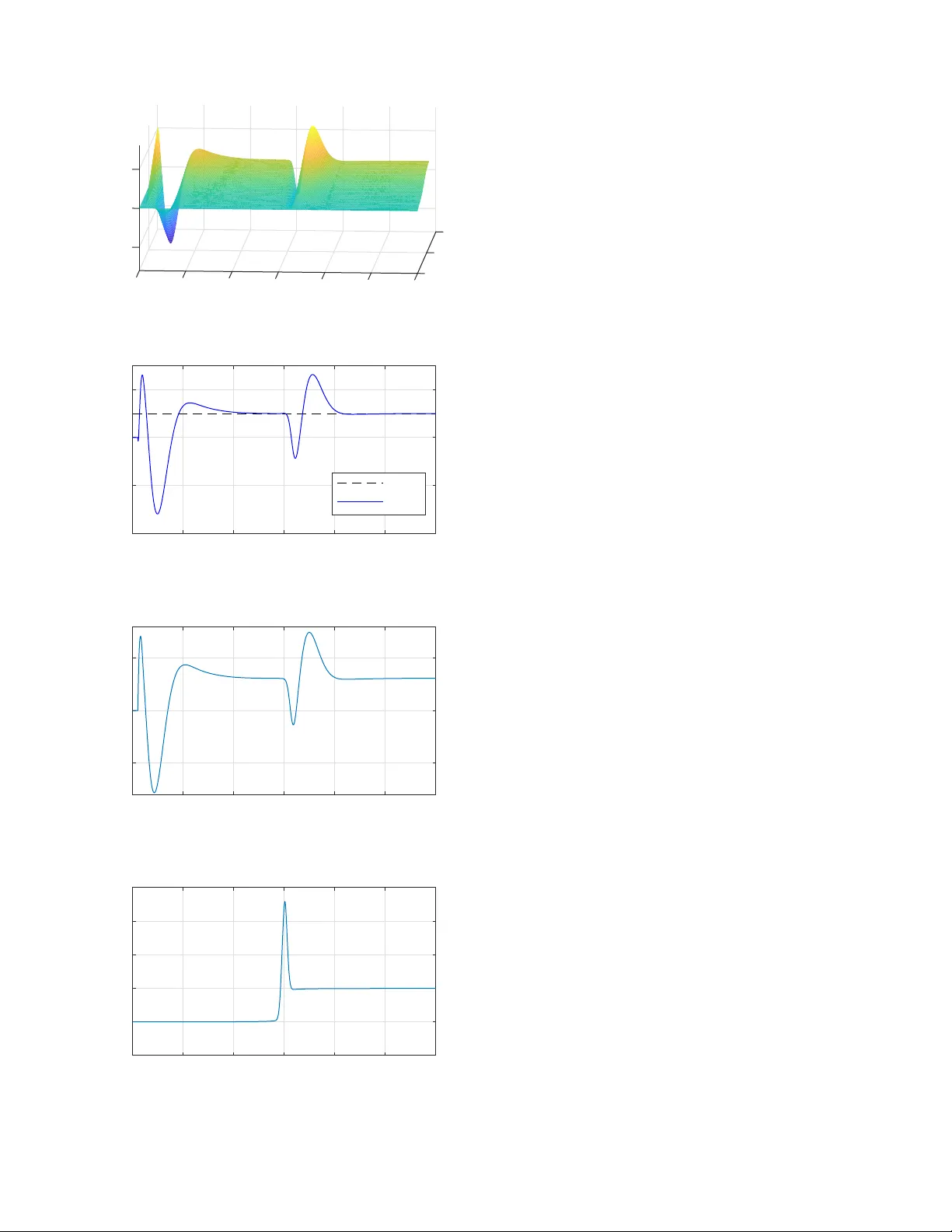
MANUSCRIPT 1 PI Re gulation of a Reaction-Dif fusion Equation with Delayed Boundary Control Hugo Lhachemi, Christophe Prieur , Emmanuel T r ´ elat Abstract —The general context of this work is the feedback control of an infinite-dimensional system so that the closed- loop system satisfies a fading-memory property and achieves the setpoint tracking of a given refer ence signal. Mor e specif- ically , this paper is concerned with the Proportional Integral (PI) regulation control of the left Neumann trace of a one- dimensional reaction-diffusion equation with a delayed right Dirichlet boundary control. In this setting, the studied r eaction- diffusion equation might be either open-loop stable or unstable. The proposed control strategy goes as follows. First, a finite- dimensional truncated model that captur es the unstable dynamics of the original infinite-dimensional system is obtained via spectral decomposition. The truncated model is then augmented by an integral component on the tracking error of the left Neumann trace. After resorting to the Artstein transf ormation to handle the control input delay , the PI controller is designed by pole shifting. Stability of the r esulting closed-loop infinite-dimensional system, consisting of the original reaction-diffusion equation with the PI controller , is then established thanks to an adequate L yapunov function. In the case of a time-varying reference input and a time-varying distributed disturbance, our stability result takes the form of an exponential Input-to-State Stability (ISS) estimate with fading memory . Finally , another exponential ISS estimate with fading memory is established for the tracking perf ormance of the refer ence signal by the system output. In particular , these results assess the setpoint regulation of the left Neumann trace in the presence of distributed perturbations that con verge to a steady-state value and with a time-deriv ative that con v erges to zero. Numerical simulations are carried out to illustrate the efficiency of our control strategy . Index T erms —1-D reaction-diffusion equation, PI regulation control, Neumann trace, Delay boundary control, P artial Differ - ential Equations (PDEs). I . I N T RO D U C T I O N A. State of the art Motiv ated by the efficienc y of Proportional-Integral (PI) controllers for the stabilization and regulation control of finite- dimensional systems, as well as its widespread adoption by industry [2], [3], the opportunity of using PI controllers in the context of infinite-dimensional systems has attracted much attention in the recent years. One of the early attempts in This publication has emanated from research supported in part by a research grant from Science Foundation Ireland (SFI) under grant number 16/RC/3872 and is co-funded under the European Regional Development Fund and by I-Form industry partners. Hugo Lhachemi is with the School of Electrical and Electronic Engineering, Univ ersity College Dublin, Dublin, Ireland (e-mail: hugo.lhachemi@ucd.ie). Christophe Prieur is with Universit ´ e Grenoble Alpes, CNRS, Grenoble- INP , GIPSA-lab, F-38000, Grenoble, France (e-mail: christophe.prieur@gipsa- lab .fr). Emmanuel Tr ´ elat is with Sorbonne Universit ´ e, CNRS, Universit ´ e de Paris, Inria, Laboratoire Jacques-Louis Lions (LJLL), F-75005 Paris, France (email: emmanuel.trelat@sorbonne-univ ersite.fr). this area was reported in [19], [20], then extended in [30], for bounded control operators. More recently , a number of works have been reported on the PI boundary control of linear hyperbolic systems [5], [11], [15], [31]. The use of a PI boundary controller for 1-D nonlinear transport equation has been studied first in [29] and then extended in [8]. In particular , the former tackled the regulation problem for a constant reference input and in the presence of constant perturbations. The regulation of the do wnside angular velocity of a drilling string with a PI controller w as reported in [28]. The considered model consists of a wa ve equation coupled with ODEs in the presence of a constant disturbance. A related problem, the PI control of a drilling pipe under friction, was in vestigated in [4]. Recently , the opportunity to add an inte gral component to open-loop exponentially stable semigroups for the output tracking of a constant reference input and in the presence of a constant distributed perturbation was in vestigated in [26], [27] for unbounded control operators by using a L yapunov functional design procedure. In this paper , we are concerned with the PI regulation con- trol of the left Neumann trace of a one-dimensional reaction- diffusion equation with a delayed right Dirichlet boundary control. Specifically , we aim at achie ving the setpoint reference tracking of a time-v arying reference signal in spite of both the presence of an arbitrarily large constant input delay and a time- varying distributed disturbance. One of the early contributions regarding stabilization of PDEs with an arbitrarily large input delay deals with a reaction-dif fusion equation [14] where the controller was designed by resorting to the backstepping technique. A different approach, which is the one adopted in this paper , takes adv antage of the following control design procedure initially reported in [23] and later used in [9], [10], [24] to stabilize semilinear heat, w av e or fluid equations via (undelayed) boundary feedback control: 1) design of the controller on a finite-dimensional model capturing the unstable modes of the original infinite-dimensional system; 2) use of an adequate L yapunov function to assess that the designed control la w stabilizes the whole infinite-dimensional system. The extension of this design procedure to the delay feedback control of a one-dimensional linear reaction-diffusion equation was reported in [21]. The impact of the input-delay was handled in the control design by the synthesis of a predictor feedback via the classical Artstein transformation [1], [22] (see also [6]). This control strategy was replicated in [12] for the feedback stabilization of a linear Kuramoto-Si vashinsky equation with delay boundary control. This idea was then generalized to the boundary feedback stabilization of a class of diagonal infinite-dimensional systems with delay boundary MANUSCRIPT 2 control for either a constant [16], [18] or a time-varying [17] input delay . B. In vestigated control pr oblem Let L > 0 , let c ∈ L ∞ (0 , L ) and let D > 0 be arbitrary . W e consider the one-dimensional reaction-diffusion equation ov er (0 , L ) with delayed Dirichlet boundary control: y t = y xx + c ( x ) y + d ( t, x ) , ( t, x ) ∈ R ∗ + × (0 , L ) (1a) y ( t, 0) = 0 , t > 0 (1b) y ( t, L ) = u D ( t ) , u ( t − D ) , t > 0 (1c) y (0 , x ) = y 0 ( x ) , x ∈ (0 , L ) (1d) where y ( t, · ) ∈ L 2 (0 , L ) is the state at time t , u ( t ) ∈ R is the control input, D > 0 is the (constant) control input delay , and d ( t, · ) ∈ L 2 (0 , L ) is a time-varying distributed disturbance, continuously differentiable with respect to t . In this paper , our objective is to achiev e the PI re gulation control of the left Neumann trace y x ( t, 0) to some prescribed reference signal, in the presence of the time-varying distributed disturbance d . More precisely , let r : R + → R be an arbitrary continuous function (reference signal). W e aim at achieving the setpoint tracking of the time-v arying reference signal r ( t ) by the left Neumann trace y x ( t, 0) . Note that an exponentially stabilizing controller for (1a-1d) was designed in [21] in the disturbance-free case ( d = 0 ) for a system trajectory ev aluated in H 1 0 -norm. The control strategy that we develop in the present paper elaborates on the one of [21], adequately combined with a PI procedure. First, a finite-dimensional model capturing all unstable modes of the original infinite-dimensional system is obtained by an appropriate spectral decomposition. Following the standard PI approach, the tracking error on the left Neumann trace is then added as a new component to the resulting finite-dimensional system. Before synthetizing the PI controller, the control input delay is handled thanks to the Artstein transformation. A predictor feedback control, obtained by pole shifting, is then designed to exponentially stabilize the aforementioned truncated model. The core of the proof consists of establishing that this PI feedback controller exponentially stabilizes as well the complete infinite-dimensional system. This is done by an appropriate L yapunov-based argument. The obtained results take the form of exponential Input-to-State Stability (ISS) estimates [25] with fading memory of the reference input and the distributed perturbation. In the case where r ( t ) → r e , d ( t ) → d e and ˙ d ( t ) → 0 when t → + ∞ , these estimates ensure the conv ergence of the state of the system, as well as the fulfillment of the desired setpoint regulation y x ( t, 0) → r e . The paper is organized as follows. The proposed control strategy is introduced in Section II. The study of the equi- librium points of the closed-loop system and the associated dynamics are presented in Section III. Then, the stability analysis of the closed-loop system is presented in Section IV while the assessment of the tracking performance is reported in Section V. The obtained results are illustrated by numerical simulations in Section VI. Finally , concluding remarks are formulated in Section VII. I I . C O N T RO L D E SI G N S T R A T E G Y The sets of nonneg ativ e integers, positi ve integers, real, non- negati ve real, and positive real are denoted by N , N ∗ , R , R + , and R ∗ + , respectiv ely . All the finite-dimensional spaces R p are endowed with the usual Euclidean inner product h x, y i = x > y and the associated 2-norm k x k = p h x, x i = √ x > x . For any matrix M ∈ R p × q , k M k stands for the induced norm of M associated with the abov e 2-norms. For a giv en symmetric matrix P ∈ R p × p , λ m ( P ) and λ M ( P ) denote its smallest and lar gest eigen values, respecti vely . In the sequel, the time deriv ative ∂ f /∂ t is either denoted by f t or ˙ f while the spatial deriv ative ∂ f /∂ x is either denoted by f x or f 0 . A. Augmented system for PI feedback contr ol The control design objecti ve is: 1) to stabilize the reaction- diffusion system (1a-1d); 2) to ensure the setpoint tracking of the reference signal r ( t ) by the left Neumann trace y x ( t, 0) . W e address this problem by designing a PI controller . Fol- lowing the general PI scheme, we augment the system by introducing a new state z ( t ) ∈ R taking the form of the integral of the tracking error y x ( t, 0) − r ( t ) (as for finite-dimensional systems, the objectiv e of this integral component is to ensure the setpoint tracking of the reference signal in the presence of the distributed disturbance d ): y t = y xx + c ( x ) y + d ( t, x ) , ( t, x ) ∈ R ∗ + × (0 , L ) (2a) ˙ z ( t ) = y x ( t, 0) − r ( t ) , t > 0 (2b) y ( t, 0) = 0 , t > 0 (2c) y ( t, L ) = u D ( t ) , u ( t − D ) , t > 0 (2d) y (0 , x ) = y 0 ( x ) , x ∈ (0 , L ) (2e) z (0) = z 0 (2f) where z 0 ∈ R stands for the initial condition of the integral component. As we are only concerned in prescribing the future of the system, we assume that the system is uncontrolled for t < 0 , i.e., u ( t ) = 0 for t < 0 . Consequently , due to the input delay D > 0 , the system is in open loop over the time range [0 , D ) as the impact of the control strategy actually applies in the boundary condition only for t > D . B. Modal decomposition It is con venient to rewrite (2a-2f) as an equi valent homo- geneous Dirichlet problem. Specifically , assuming 1 that u is continuously differentiable and setting w ( t, x ) = y ( t, x ) − x L u D ( t ) , we have w t = w xx + c ( x ) w + x L c ( x ) u D − x L ˙ u D ( t ) + d ( t, x ) (3a) ˙ z ( t ) = w x ( t, 0) + 1 L u D ( t ) − r ( t ) (3b) w ( t, 0) = w ( t, L ) = 0 (3c) w (0 , x ) = y 0 ( x ) − x L u D (0) (3d) z (0) = z 0 (3e) 1 This property will be ensured by the construction carried out in the sequel. MANUSCRIPT 3 for t > 0 and x ∈ (0 , 1) . W e consider the real state- space L 2 (0 , 1) endowed with its usual inner product h f , g i = R L 0 f ( x ) g ( x ) d x . Introducing the operator A = ∂ xx + c id : D ( A ) ⊂ L 2 (0 , L ) → L 2 (0 , L ) defined on the domain D ( A ) = H 2 (0 , L ) ∩ H 1 0 (0 , L ) , (3a-3c) can be rewritten as w t ( t, · ) = A w ( t, · ) + a ( · ) u D ( t ) + b ( · ) ˙ u D ( t ) + d ( t, · ) (4a) ˙ z ( t ) = w x ( t, 0) + 1 L u D ( t ) − r ( t ) (4b) with a ( x ) = x L c ( x ) and b ( x ) = − x L for ev ery x ∈ (0 , L ) , with initial conditions (3d-3e). Since A is self-adjoint and of compact resolvent, we consider a Hilbert basis ( e j ) j > 1 of L 2 (0 , L ) consisting of eigenfunctions of A associated with the sequence of real eigen values −∞ < · · · < λ j < · · · < λ 1 with λ j − → j → + ∞ −∞ . Note that e j ( · ) ∈ H 1 0 (0 , L ) ∩ C 2 ([0 , L ]) for ev ery j > 1 and e 0 j (0) ∼ r 2 L q | λ j | , λ j ∼ − π 2 j 2 L 2 , (5) when j → + ∞ . The solution w ( t, · ) ∈ H 2 (0 , L ) ∩ H 1 0 (0 , L ) of (4a) can be expanded as a series in the eigenfunctions e j ( · ) , con ver gent in H 1 0 (0 , L ) , w ( t, · ) = + ∞ X j =1 w j ( t ) e j ( · ) . (6) Therefore (4a-4b) is equiv alent to the infinite-dimensional control system: ˙ w j ( t ) = λ j w j ( t ) + a j u D ( t ) + b j ˙ u D ( t ) + d j ( t ) (7a) ˙ z ( t ) = X j > 1 w j ( t ) e 0 j (0) + 1 L u D ( t ) − r ( t ) (7b) for j ∈ N ∗ , with w j ( t ) = h w ( t, · ) , e j i = Z L 0 w ( t, x ) e j ( x ) d x, a j = h a, e j i = 1 L Z L 0 xc ( x ) e j ( x ) d x, b j = h b, e j i = − 1 L Z L 0 xe j ( x ) d x, d j ( t ) = h d ( t, · ) , e j i = Z L 0 d ( t, x ) e j ( x ) d x. Introducing the auxiliary control input v , ˙ u , and denoting v D ( t ) , v ( t − D ) , (7a-7b) can be rewritten as ˙ u D ( t ) = v D ( t ) (8a) ˙ w j ( t ) = λ j w j ( t ) + a j u D ( t ) + b j v D ( t ) + d j ( t ) (8b) ˙ z ( t ) = X j > 1 w j ( t ) e 0 j (0) + 1 L u D ( t ) − r ( t ) (8c) for j ∈ N ∗ . Since u ( t ) = 0 for t < 0 , (8a) imposes that the auxiliary control input is such that v ( t ) = 0 for t < 0 , and that the corresponding initial condition satisfies u D (0) = u ( − D ) = 0 . In the sequel, we design the control law v in order to stabilize (8a-8c). In this context, the actual control input u associated with the original system (2a-2f) is u ( t ) = R t 0 v ( τ ) d τ for ev ery t > 0 . C. F inite-dimensional truncated model In what follows, we fix the integer n ∈ N such that λ n +1 < 0 6 λ n . In particular , we have λ j > 0 when 1 6 j 6 n and λ j 6 λ n +1 < 0 when j > n + 1 . Remark 1: In the case of an open-loop stable reaction- diffusion equation, we have n = 0 . In this particular case, as discussed in the sequel, the objectiv e of the control design is to ensure the output regulation while preserving the stability of the closed-loop system. ◦ Let us first sho w how to obtain a finite-dimensional trun- cated model capturing the n first modes of the reaction diffusion-equation. W e follow [21]. Setting X 1 ( t ) =      u D ( t ) w 1 ( t ) . . . w n ( t )      , A 1 =      0 0 · · · 0 a 1 λ 1 · · · 0 . . . . . . . . . . . . a n 0 · · · λ n      , B 1 =  1 b 1 . . . b n  > , D 1 ( t ) =  0 d 1 ( t ) . . . d n ( t )  > , with X 1 ( t ) ∈ R n +1 , A 1 ∈ R ( n +1) × ( n +1) , B 1 ∈ R n +1 , D 1 ( t ) ∈ R n +1 , (8a) and the n first equations of (8b) yield ˙ X 1 ( t ) = A 1 X 1 ( t ) + B 1 v D ( t ) + D 1 ( t ) . (9) W e could now augment the state-vector X 1 to include the integral component z in the control design. Ho wev er , the time deriv ative of z , giv en by (8c), in volv es all coefficients w j ( t ) , j > 1 . Thus, the direct augmentation of the state vector X 1 with the integral component z does not allo w the deriv ation of an ODE inv olving only the n first modes of the reaction- diffusion equation. T o overcome this issue, we set ζ ( t ) , z ( t ) − X j > n +1 e 0 j (0) λ j w j ( t ) . (10) Noting that    e 0 j (0) λ j    2 ∼ 2 L π 2 j 2 when j → + ∞ and thus that ( e 0 j (0) /λ j ) j and ( w j ( t )) j are square summable sequences, using the Cauchy-Schwarz inequality , we see that the series (10) is con vergent and that ˙ ζ ( t ) = ˙ z ( t ) − X j > n +1 e 0 j (0) λ j ˙ w j ( t ) = αu D ( t ) + β v D ( t ) − γ ( t ) + n X j =1 w j ( t ) e 0 j (0) , where we have used (8b-8c), with α = 1 L − X j > n +1 e 0 j (0) λ j a j , β = − X j > n +1 e 0 j (0) λ j b j , (11a) γ ( t ) = r ( t ) + X j > n +1 e 0 j (0) λ j d j ( t ) . (11b) MANUSCRIPT 4 The con ver gence of the abov e series follo w again by the Cauchy-Schwarz inequality . Then we have ˙ ζ ( t ) = L 1 X 1 ( t ) + β v D ( t ) − γ ( t ) (12) with L 1 =  α e 0 1 (0) . . . e 0 n (0)  ∈ R 1 × ( n +1) . Now , defin- ing the augmented state-vector X ( t ) =  X 1 ( t ) > ζ ( t )  > ∈ R n +2 , the exogenous input Γ( t ) =  D 1 ( t ) > − γ ( t )  > ∈ R n +2 and the matrices A =  A 1 0 L 1 0  ∈ R ( n +2) × ( n +2) , B =  B 1 β  ∈ R n +2 , (13) we obtain from (9) and (12) the control system ˙ X ( t ) = AX ( t ) + B v D ( t ) + Γ( t ) (14) which is the finite-dimensional truncated model capturing the unstable part of the infinite-dimensional augmented with an integral component for generating the actual control input and an integral component for setpoint reference tracking. In particular , the system (14) only inv olves the n first modes of the reaction-diffusion equation. Remark 2: The above developments allow the particular case n = 0 , which corresponds to the configuration where (1a-1d) is open-loop stable. In this configuration, the vectors and matrices of the truncated model (14) reduce to X ( t ) =  u D ( t ) ζ ( t )  > ∈ R 2 , Γ( t ) =  1 − γ ( t )  > ∈ R 2 , A =  0 0 α 0  , B =  1 β  . In this setting, the control objectiv e consists of ensuring the setpoint tracking of the system output y x ( t, 0) while preserving the stability of the closed-loop system. ◦ Putting together the finite-dimensional truncated model (14) along with (8b) for j > n + 1 which correspond to the modes of the original infinite-dimensional system neglected by the truncated model, we get the final representation used for both control design and stability analyses: ˙ X ( t ) = AX ( t ) + B v D ( t ) + Γ( t ) (15a) ˙ w j ( t ) = λ j w j ( t ) + a j u D ( t ) + b j v D ( t ) + d j ( t ) (15b) with j > n + 1 . D. Contr ollability of the finite-dimensional truncated model As mentioned in the introduction, the control design strategy relies now on the two following steps. First, we want to design a controller for the finite-dimensional system (14). Second, we aim at assessing that the obtained PI controller successfully stabilizes the original infinite-dimensional system (2a-2f) and provides the desired setpoint reference tracking. In order to fulfill the first objectiv e, we first establish the controllability property for the pair ( A, B ) . Lemma 1: The pair ( A, B ) satisfies the Kalman condition. Proof: Considering the structures of A and B defined by (13), we apply Lemma 7 reported in Appendix. More specifically , from the implication ( i ) ⇒ ( ii ) , we need to check that the pair ( A 1 , B 1 ) satisfies the Kalman condi- tion and the square matrix  A 1 B 1 L 1 β  is inv ertible. The first condition is indeed true as straightforward computa- tions show that det ( B 1 , A 1 B 1 , . . . , A n 1 B 1 ) = Q n j =1 ( a j + λ j b j )VdM( λ 1 , . . . , λ n ) 6 = 0 , where VdM is a V andermonde determinant, because all eigen values are distinct and, using A e j = λ j e j and an inte gration by parts, a j + λ j b j = − e 0 j ( L ) 6 = 0 by Cauchy uniqueness (see also [21]). Thus, we focus on the in vertibility condition: det  A 1 B 1 L 1 β  = det        0 0 · · · 0 1 a 1 λ 1 · · · 0 b 1 . . . . . . . . . . . . . . . a n 0 · · · λ n b n α e 0 1 (0) · · · e 0 n (0) β        = ( − 1) n +1 det      a 1 λ 1 · · · 0 . . . . . . . . . . . . a n 0 · · · λ n α e 0 1 (0) · · · e 0 n (0)      . W e now consider two distinct cases depending on whether λ = 0 is an eigen value of A or not. Let us first consider the case where λ = 0 is not an eigen v alue of A . In particular , λ 1 , . . . , λ n are all non zero and thus row operations applied to the last row yield: det  A 1 B 1 L 1 β  = ( − 1) n +1 det        a 1 λ 1 · · · 0 . . . . . . . . . . . . a n 0 · · · λ n α − n P i =1 a i e 0 i (0) λ i 0 · · · 0        = − α − n X i =1 a i e 0 i (0) λ i ! n Y j =1 λ j . Consequently , based on the definition of the constant α giv en by (11a), the abov e determinant is not zero if and only if X j > 1 a i e 0 i (0) λ i 6 = 1 L . (16) W e note that this condition is independent of the number n of modes of the infinite-dimensional system captured by the truncated model and we show in the sequel that (16) always holds true. T o do so, let y e be the stationary solution of (1a-1d) associated with the constant boundary input u e = 1 and zero distributed disturbance, i.e., ( y e ) xx + cy e = 0 with y e (0) = 0 and y e ( L ) = 1 . Such a function y e indeed exists and can be obtained as follo ws. By assumption, λ = 0 is not an eigen value of A . Thus the solution y 0 of ( y 0 ) xx + cy 0 = 0 with y 0 (0) = 0 and y 0 0 (0) = 1 satisfies y 0 ( L ) 6 = 0 . Hence, one can obtain the claimed function by defining y e ( x ) = y 0 ( x ) /y 0 ( L ) . Now , w e ( x ) , y e ( x ) − x L is a stationary solution of (3a) and (3c- 3d) in the sense that ( w e ) xx + cw e + x L c = 0 with w e (0) = w e ( L ) = 0 . From (7a), λ j w e,j + a j = 0 and thus w e,j = − a j λ j . W e deduce that ( w e ) x (0) = X j > 1 w e,j e 0 j (0) = − X j > 1 a j λ j e 0 j (0) . Hence (16) holds if and only if ( w e ) x (0) 6 = − 1 L , which is equi valent to ( y e ) x (0) 6 = 0 . By Cauchy uniqueness, the MANUSCRIPT 5 condition ( y e ) x (0) = 0 , along with ( y e ) xx + cy e = 0 and y e (0) = 0 , implies that y e = 0 , which contradicts y e ( L ) = 1 . Thus (16) holds and the system is controllable. Let us no w consider the second case, i.e., λ = 0 is an eigen v alue of A . Based on the definition of the integer n , we hav e n > 1 and λ n = 0 while λ k > 0 for all 1 6 k 6 n − 1 . Expanding the determinant, first, along the ( n + 1) -th column, and then, along the n -th row , we obtain det  A 1 B 1 L 1 β  = a n e 0 n (0) n − 1 Y i =1 λ i . By Cauchy uniqueness, we hav e e 0 n (0) 6 = 0 (otherwise e n would be solution of a second-order ODE with the boundary conditions e n (0) = e 0 n (0) = 0 , yielding the contradiction e n = 0 ). Thus, the above determinant is nonzero if and only if a n 6 = 0 . W e proceed by contradiction. Using e 00 n + ce n = A e n = 0 and a n = 1 L R L 0 xc ( x ) e n ( x ) d x = 0 , we obtain by integration by parts: 0 = − R L 0 xe 00 n ( x ) d x = − [ xe 0 n ( x )] x = L x =0 + R L 0 e 0 n ( x ) d x = − Le 0 n ( L ) , whence e 0 n ( L ) = 0 . This result, along with e 00 n + ce n = 0 and e n ( L ) = 0 , yields by Cauchy uniqueness the contradiction e n = 0 . Thus, a n 6 = 0 and the system is controllable.  E. Contr ol design strate gy Using the controllability property of the pair ( A, B ) , we propose to resort to the classical predictor feedback to stabi- lize the finite-dimensional truncated model (15a). Specifically , introducing the Artstein transformation Z ( t ) = X ( t ) + Z t t − D e A ( t − D − τ ) B v ( τ ) d τ (17) (see [1]), straightforward computations show that ˙ Z ( t ) = AZ ( t ) + e − DA B v ( t ) + Γ( t ) . Since ( A, B ) satisfies the Kalman condition, the pair ( A, e − DA B ) also satisfies the Kalman condition and we infer the existence of a feedback gain K ∈ R 1 × ( n +2) such that A K , A + e − DA B K is Hurwitz. W e choose the control law v ( t ) = χ [0 , + ∞ ) ( t ) K Z ( t ) (18) where χ [0 , + ∞ ) denotes the characteristic function of the in- terval [0 , + ∞ ) , which is used to capture the fact that we are only concerned by imposing a non zero control input for t > 0 . Then we obtain the stable closed-loop dynamics ˙ Z ( t ) = A K Z ( t ) + Γ( t ) . Remark 3: The first component of Z ( t ) is u ( t ) . Indeed, denoting by E 1 =  1 0 . . . 0  ∈ R 1 × ( n +2) , we have E 1 Z ( t ) = E 1 X ( t ) + Z t t − D E 1 e ( t − s − D ) A B v ( s ) d s = u D ( t ) + Z t t − D v ( s ) d s = u ( t ) where we ha ve used that the first ro w of A is null, that v ( t ) = ˙ u ( t ) for t > 0 and that u ( t ) = 0 when t 6 0 . ◦ Remark 4: Putting together (17-18) and using the fact that v ( t ) = 0 for t 6 0 , we obtain that the control input v is solution of the fixed point implicit equation v ( t ) = χ [0 , + ∞ ) ( t ) K X ( t )+ K Z t max( t − D, 0) e A ( t − D − τ ) B v ( τ ) d τ . Existence and uniqueness of the solution of the above equation as well as re gularity properties and in version of the Artstein transformation are reported in [6]. ◦ The main objectiv e is now to establish that the feedback control (18) stabilizes as well the original infinite-dimensional system (or , in the case n = 0 , preserves the stability property of the system) while providing a setpoint tracking of the time-varying reference signal r ( t ) by the left Neumann trace y x ( t, 0) . The former is studied in Section IV while the latter is inv estigated in Section V. I I I . E Q U I L I B R I U M C O N D I T I O N A N D R E L A T E D DY N A M I C S In the sequel, r e ∈ R and d e ∈ L 2 (0 , L ) stand for “nominal values” of the time-v arying reference signals r ( t ) and the distributed disturbance d ( t ) , respectiv ely . Even if r e and d e can be selected arbitrarily , the two following (distinct) cases will be of particular interest in the sequel: • | r ( t ) − r e | 6 δ r and k d ( t ) − d e k 6 δ d for some δ r , δ d > 0 ; • r ( t ) → r e and d ( t ) → d e when t → + ∞ . A. Characterization of equilibrium for the closed-loop system Setting d e,j = h d e , e j i = R L 0 d e ( x ) e j ( x ) d x for j > 1 , ∆ r = r − r e , ∆ d = d − d e , ∆ d j = d j − d e,j , Γ e =         0 d e, 1 . . . d e,n − r e − P j > n +1 e 0 j (0) λ j d e,j         , ∆Γ =         0 ∆ d 1 . . . ∆ d n − ∆ r − P j > n +1 e 0 j (0) λ j ∆ d j         we obtain from (15a-15b) and (18) ˙ Z ( t ) = A K Z ( t ) + Γ e + ∆Γ( t ) ˙ w j ( t ) = λ j w j ( t ) + a j u D ( t ) + b j v D ( t ) + d e,j + ∆ d j ( t ) for j > n + 1 . W e now characterize the equilibrium condition of the above closed-loop system associated with the constant reference input r ( t ) = r e ∈ R and the constant distributed disturbance d ( t ) = d e ∈ L 2 (0 , L ) (i.e., ∆ r = 0 and ∆ d = 0 ). In the sequel, we denote by a subscript “e” the equilibrium value of the different quantities. For instance, Z e denotes the equilibrium value of Z . Noting that u D,e = u e and v D,e = v e , we obtain 0 = A K Z e + Γ e 0 = λ j w j,e + a j u e + b j v e + d e,j , j > n + 1 In particular, from v e = K Z e , we have 0 = A K Z e + Γ e = AZ e + e − DA B v e + Γ e . Since the first rows of A and Γ e are null and E 1 e − DA B = 1 , we obtain v e = 0 and Z e = − A − 1 K Γ e (19a) MANUSCRIPT 6 u e = E 1 Z e = − E 1 A − 1 K Γ e (19b) w j,e = − a j λ j u e − d e,j λ j , j > n + 1 (19c) W e introduce X e = Z e because AX e + B v D,e + Γ e = A K Z e + Γ e = 0 , which is compatible with the Artstein transformation since v e = 0 implies Z e = X e + R t t − D e ( t − s − D ) A B v e d s . The equilibrium condition of the integral component for reference tracking is giv en by ζ e = E n +2 X e = − E n +2 A − 1 K Γ e , (19d) where E n +2 =  0 . . . 0 1  ∈ R 1 × ( n +2) . Noting that λ j w j,e = − a j u e − d e,j for j > n + 1 where ( a j ) j and ( d e,j ) j are square-summable sequences and λ j → + ∞ when j → + ∞ , both ( w j,e ) j and ( λ j w j,e ) j are square-summable sequences. Hence we define w e , X j > 1 w j,e e j ∈ D ( A ) = H 2 (0 , L ) ∩ H 1 0 (0 , L ) (20) which is con vergent in H 1 0 (0 , L ) . In particular , we obtain from the last line of AX e + Γ e = 0 and using (19c) that L 1 X 1 ,e = r e + X j > n +1 e 0 j (0) λ j d e,j ⇔ 1 L u e − X j > n +1 e 0 j (0) λ j a j u e + n X j =1 w j,e e 0 j (0) = r e + X j > n +1 e 0 j (0) λ j d e,j ⇔ X j > 1 w j,e e 0 j (0) + 1 L u e = r e ⇔ w 0 e (0) + 1 L u e = r e . Then, introducing y e , w e + x L u e ∈ L 2 (0 , L ) , we obtain y 0 e (0) = r e , which corresponds to the desired reference tracking. Finally , since A w e = X j > 1 λ j w j,e e j = − X j > 1 a j e j u e − X j > 1 d e,j e j = − au e − bv e − d e , we have A w e + au D,e + bv D,e + d e = 0 . Remark 5: The above dev elopments show that the equi- librium point of the closed-loop infinite-dimensional system giv en by (19a-19d) and (20) is fully determined by the constant values of the reference signal r e and the distributed disturbance d e . ◦ B. Dynamics of deviations W e now define the deviations of the v arious quantities with respect to their equilibrium value: ∆ X = X − X e , ∆ Z = Z − Z e , ∆ w = w − w e , ∆ w j = w j − w j,e , ∆ ζ = ζ − ζ e , ∆ u = u − u e (first component of ∆ Z ), ∆ u D = u D − u e (first component of ∆ X ), ∆ v = v − v e , and ∆ v D = v D − v D,e . Then, in original coordinates: ∆ w t = A ∆ w + a ∆ u D + b ∆ v D + ∆ d (21) and ∆ ˙ X ( t ) = A ∆ X ( t ) + B ∆ v D ( t ) + ∆Γ( t ) ∆ ˙ w j ( t ) = λ j ∆ w j ( t ) + a j ∆ u D ( t ) + b j ∆ v D ( t ) + ∆ d j ( t ) for j > n + 1 with the auxiliary control input ∆ v ( t ) = χ [0 , + ∞ ) ( t ) K ∆ Z ( t ) where ∆ Z ( t ) = ∆ X ( t ) + Z t t − D e ( t − s − D ) A B ∆ v ( s ) d s. (22) In Z coordinates, the closed-loop dynamics is gi ven by ∆ ˙ Z ( t ) = A K ∆ Z ( t ) + ∆Γ( t ) (23a) ∆ ˙ w j ( t ) = λ j ∆ w j ( t ) + a j ∆ u D ( t ) + b j ∆ v D ( t ) + ∆ d j ( t ) (23b) for j > n + 1 . I V . S TA B I L I T Y A NA LY S I S A. Main stability result The objecti ve of this section is to establish the follo wing stability result, taking the form of an Input-to-State Stability (ISS) estimate with fading memory of both the reference input r and the distributed perturbation d . Theorem 1: Ther e exist κ, C 1 > 0 such that, for every  ∈ [0 , 1) , ther e exists C 2 (  ) > 0 such that ∆ u D ( t ) 2 + ∆ ζ ( t ) 2 + k ∆ w ( t ) k 2 H 1 0 (0 ,L ) (24) 6 C 1 e − 2 κt  ∆ u D (0) 2 + ∆ ζ (0) 2 + k ∆ w (0) k 2 H 1 0 (0 ,L )  + C 2 (  ) sup 0 6 s 6 t e − 2 κ ( t − s ) { ∆ r ( s ) 2 + k ∆ d ( s ) k 2 } . Mor eover , the constants κ, C 1 , C 2 (  ) can be chosen indepen- dently of r e and d e . Since ∆ w ( t, x ) = ∆ y ( t, x ) − x L ∆ u D ( t ) , we deduce from the continuous embedding H 1 0 (0 , L ) ⊂ L ∞ (0 , L ) (see, e.g., [7]) the following corollary . Corollary 1: Let κ > 0 be pr ovided by Theor em 1. Ther e exists ˜ C 1 > 0 such that, for every  ∈ [0 , 1) , there exists ˜ C 2 (  ) > 0 such that k ∆ y ( t ) k L ∞ (0 ,L ) (25) 6 ˜ C 1 e − κt  | ∆ u D (0) | + | ∆ ζ (0) | + k ∆ w (0) k H 1 0 (0 ,L )  + ˜ C 2 (  ) sup 0 6 s 6 t e − κ ( t − s ) {| ∆ r ( s ) | + k ∆ d ( s ) k} . W e also deduce the follo wing corollary concerning the asymptotic behavior of the closed-loop system in the case of con ver gent reference signal r ( t ) and distributed disturbance d ( t ) as t → + ∞ . Corollary 2: Assume that r ( t ) → r e and d ( t ) → d e when t → + ∞ . Then w ( t ) → w e in H 1 0 norm, y ( t ) → y e in both L ∞ and L 2 norm, u ( t ) → u e , and ζ ( t ) → ζ e with exponential vanishing of the contribution of the initial conditions. Remark 6: In the particular case n = 0 , which corresponds to an exponentially stable open-loop reaction-diffusion equa- tion (1a-1d), the above results ensure that the stability of the closed-loop system is preserved after introduction of the two integral states v and z . ◦ MANUSCRIPT 7 In order to prove the claimed stability result, we resort as in [21] to the L yapunov function V ( t ) = M 2 ∆ Z ( t ) > P ∆ Z ( t ) (26) + M 2 Z t max( t − D, 0) ∆ Z ( s ) > P ∆ Z ( s ) d s − 1 2 X j > 1 λ j ∆ w j ( t ) 2 , where P ∈ R ( n +2) × ( n +2) is the solution of the L yapunov equation A > K P + P A K = − I and M > 0 is chosen such that M > max  γ 1 λ 1 λ m ( P ) , 4  γ 1 k a k 2 + 2 k b k 2 k e − DA K k 2 k K k 2   with γ 1 , 2 max  1 , D e 2 D k A k k B K k 2  . Remark 7: The first term in the definition (26) of V accounts for the stability of the finite-dimensional truncated model (23a), e xpressed in Z coordinates, capturing the n first modes of the reaction-diffusion equation. The motiv ation be- hind the introduction of the second (integral) term relies on the fact that it allows, in conjunction with (22), the deriv ation of an upper-estimate of k ∆ X ( t ) k (i.e., the state of the truncated model in its original X coordinates) based on V ( t ) . Finally , the last term is used to capture the countable infinite number of modes of the original reaction-dif fusion equation (21), including those that where neglected in the control design. Note that hA ∆ w ( t ) , ∆ w ( t ) i = P j > 1 λ j ∆ w j ( t ) 2 . ◦ B. Pr eliminary Lemmas for the pr oof of Theor em 1 W e deriv e hereafter v arious lemmas that will be useful in the sequel to establish the stability properties of the closed-loop system. First, we estimate ∆Γ( t ) as follows. Lemma 2: Ther e exists a constant M d > 0 such that k ∆Γ( t ) k 2 6 M 2 d (∆ r ( t ) 2 + k ∆ d ( t ) k 2 ) ∀ t > 0 . Proof: By definition of ∆Γ( t ) and using the Cauchy- Schwarz inequality we have k ∆Γ( t ) k 2 = k ∆ D 1 ( t ) k 2 +       ∆ r ( t ) + X j > n +1 e 0 j (0) λ j ∆ d j ( t )       2 6 n X j =1 ∆ d j ( t ) 2 + 2∆ r ( t ) 2 + 2 X j > n +1     e 0 j (0) λ j     2 X j > n +1 ∆ d j ( t ) 2 6 M 2 d (∆ r ( t ) 2 + k ∆ d ( t ) k 2 ) with M 2 d = 2 max 1 , P j > n +1    e 0 j (0) λ j    2 ! < + ∞ , since, by (5), we have    e 0 j (0) λ j    2 ∼ 2 L π 2 j 2 when j → + ∞ .  Lemma 3: Ther e exists a constant C 1 > 0 such that V ( t ) > C 1 X j > 1 (1 + | λ j | )∆ w j ( t ) 2 , (27a) V ( t ) > C 1  ∆ u D ( t ) 2 + ∆ ζ ( t ) 2 + k ∆ w ( t ) k 2 H 1 0 (0 ,L )  , (27b) V ( t ) > C 1 k ∆ Z ( t ) k 2 , (27c) for every t > 0 . Proof: From (22) with ∆ v = K ∆ Z , we obtain that k ∆ X ( t ) k 2 6 2 k ∆ Z ( t ) k 2 + 2 D e 2 D k A k k B K k 2 Z t max( t − D, 0) k ∆ Z ( s ) k 2 d s 6 γ 1 k ∆ Z ( t ) k 2 + Z t max( t − D, 0) k ∆ Z ( s ) k 2 d s ! (28) with γ 1 = 2 max  1 , D e 2 D k A k k B K k 2  > 0 . Thus, we hav e ∆ Z ( t ) > P ∆ Z ( t ) + Z ( t − D,t ) ∩ (0 , + ∞ ) ∆ Z ( s ) > P ∆ Z ( s ) d s > λ m ( P ) γ 1 k ∆ X ( t ) k 2 . Noting that X j > 1 λ j ∆ w j ( t ) 2 6 X j > n +1 λ j ∆ w j ( t ) 2 + λ 1 n X j =1 ∆ w j ( t ) 2 6 X j > n +1 λ j ∆ w j ( t ) 2 + λ 1 k ∆ X ( t ) k 2 , we obtain V ( t ) >  M λ m ( P ) 2 γ 1 − λ 1 2  k ∆ X ( t ) k 2 − 1 2 X j > n +1 λ j ∆ w j ( t ) 2 . Since M > γ 1 λ 1 λ m ( P ) > 0 , we obtain the existence of γ 2 = 1 2 min  M λ m ( P ) γ 1 − λ 1 , 1  > 0 such that V ( t ) > γ 2  k ∆ X ( t ) k 2 − X j > n +1 λ j ∆ w j ( t ) 2  , (29) from which we obtain (27a). Now , as in [21], from the series expansions (6) and (20) that are con ver gent in H 1 0 (0 , L ) , we infer that k ∆ w ( t ) k 2 H 1 0 (0 ,L ) = X i,j > 1 ∆ w i ( t )∆ w j ( t ) Z L 0 e 0 i ( x ) e 0 j ( x ) d x = Z L 0 c ( x )∆ w ( t, x ) 2 d x − X j > 1 λ j ∆ w j ( t ) 2 , (30) where the second equality follows from an integration by part and the facts that e 00 j + ce j = λ j e j , e j (0) = e j ( L ) = 0 , and ( e i ) i > 1 is a Hilbert basis of L 2 (0 , L ) . Hence, using the fact that − P 1 6 j 6 n λ j ∆ w j ( t ) 2 6 0 , the following estimates hold: k ∆ w ( t ) k 2 H 1 0 (0 ,L ) 6 k c k L ∞ (0 ,L ) X j > 1 ∆ w j ( t ) 2 − X j > n +1 λ j ∆ w j ( t ) 2 6 k c k L ∞ (0 ,L ) n X j =1 ∆ w j ( t ) 2 − X j > n +1  λ j − k c k L ∞ (0 ,L )  ∆ w j ( t ) 2 6 γ 3  n X j =1 ∆ w j ( t ) 2 − X j > n +1 λ j ∆ w j ( t ) 2  MANUSCRIPT 8 for some constant γ 3 > 0 because λ j − → j → + ∞ −∞ whence −  λ j − k c k L ∞ (0 ,L )  ∼ − λ j when j → + ∞ with λ j < 0 for all j > n + 1 . Therefore, we obtain from (29) that V ( t ) > γ 2  ∆ u D ( t ) 2 + ∆ ζ ( t ) 2  + γ 2 γ 3 k ∆ w ( t ) k 2 H 1 0 (0 ,L ) , which provides (27b). Finally , from the definition of V gi ven by (26) and using (28), we also hav e V ( t ) > M λ m ( P ) 2 k ∆ Z ( t ) k 2 + Z t max( t − D, 0) k ∆ Z ( s ) k 2 d s ! − 1 2 X j > n +1 λ j ∆ w j ( t ) 2 | {z } > 0 − λ 1 2 k ∆ X ( t ) k 2 > 1 2 ( M λ m ( P ) − λ 1 γ 1 ) × k ∆ Z ( t ) k 2 + Z t max( t − D, 0) k ∆ Z ( s ) k 2 d s ! > γ 1 γ 2 k ∆ Z ( t ) k 2 , which gives (27c).  C. End of pr oof of Theorem 1 W e are now in a position to establish the stability properties of the closed-loop system and prove Theorem 1. W e first study the exponential decay properties of V for t > D . Lemma 4: Ther e exist κ, C 2 > 0 such that, for every  ∈ [0 , 1) , V ( t ) 6 e − 2 κ ( t − D ) V ( D ) + C 2 1 −  sup 0 6 s 6 t e − 2 κ ( t − s )  ∆ r ( s ) 2 + k ∆ d ( s ) k 2  for every t > D . Proof: First, we note that, for t > D , d d t  Z t t − D ∆ Z ( s ) > P ∆ Z ( s ) d s  = ∆ Z ( t ) > P ∆ Z ( t ) − ∆ Z ( t − D ) > P ∆ Z ( t − D ) = Z t t − D d d τ  ∆ Z ( τ ) > P ∆ Z ( τ )  ( s ) d s. Since A is self-adjoint and since hA ∆ w ( t ) , ∆ w ( t ) i = P j > 1 λ j ∆ w j ( t ) 2 , we have for every t > D , ˙ V ( t ) = M 2 ∆ Z ( t ) >  A > K P + P A K  ∆ Z ( t ) + M ∆ Z ( t ) > P ∆Γ( t ) + M 2 Z t t − D ∆ Z ( s ) >  A > K P + P A K  ∆ Z ( s ) d s + M Z t t − D ∆ Z ( s ) > P ∆Γ( s ) d s − hA ∆ w ( t ) , ∆ w t ( t ) i = − M 2 k ∆ Z ( t ) k 2 + M ∆ Z ( t ) > P ∆Γ( t ) − M 2 Z t t − D k ∆ Z ( s ) k 2 d s + M Z t t − D ∆ Z ( s ) > P ∆Γ( s ) d s − kA ∆ w ( t ) k 2 L 2 (0 ,L ) − hA ∆ w ( t ) , a i ∆ u D ( t ) − hA ∆ w ( t ) , b i ∆ v D ( t ) − hA ∆ w ( t ) , ∆ d ( t ) i . Using the following estimates: ∆ Z ( t ) > P ∆Γ( t ) 6 k ∆ Z ( t ) kk P kk ∆Γ( t ) k 6 1 4 k ∆ Z ( t ) k 2 + k P k 2 M 2 d (∆ r ( t ) 2 + k ∆ d ( t ) k 2 ) , Z t t − D ∆ Z ( s ) > P ∆Γ( s ) d s 6 Z t t − D k ∆ Z ( s ) kk P kk ∆Γ( s ) k d s 6 1 4 Z t t − D k ∆ Z ( s ) k 2 d s + D k P k 2 M 2 d sup t − D 6 s 6 t { ∆ r ( s ) 2 + k ∆ d ( s ) k 2 } , |hA ∆ w ( t ) , a i ∆ u D ( t ) | 6 1 4 kA ∆ w ( t ) k 2 L 2 (0 ,L ) + k a k 2 | ∆ u D ( t ) | 2 6 1 4 kA ∆ w ( t ) k 2 L 2 (0 ,L ) + k a k 2 k ∆ X ( t ) k 2 6 1 4 kA ∆ w ( t ) k 2 L 2 (0 ,L ) + γ 1 k a k 2  k ∆ Z ( t ) k 2 + Z t t − D k ∆ Z ( s ) k 2 d s  , |hA ∆ w ( t ) , b i ∆ v D ( t ) | 6 1 4 kA ∆ w ( t ) k 2 L 2 (0 ,L ) + k b k 2 | ∆ v D ( t ) | 2 6 1 4 kA ∆ w ( t ) k 2 L 2 (0 ,L ) + k b k 2 k K k 2 k ∆ Z ( t − D ) k 2 6 1 4 kA ∆ w ( t ) k 2 L 2 (0 ,L ) + 2 k b k 2 k e − DA K k 2 k K k 2 k ∆ Z ( t ) k 2 + 2 M 2 d D 2 e 2 D k A K k k b k 2 k K k 2 sup t − D 6 s 6 t { ∆ r ( s ) 2 + k ∆ d ( s ) k 2 } , where we hav e used in the latter inequality that ∆ ˙ Z ( t ) = A K ∆ Z ( t ) + ∆Γ( t ) whence ∆ Z ( t − D ) = e − DA K ∆ Z ( t ) + Z t − D t e ( t − D − s ) A K ∆Γ( s )d s, and |hA ∆ w ( t ) , ∆ d ( t ) i| 6 1 4 kA ∆ w ( t ) k 2 L 2 (0 ,L ) + k ∆ d ( t ) k 2 , we obtain that, for every t > D , ˙ V ( t ) 6  − M 4 + γ 1 k a k 2 + 2 k b k 2 k e − DA K k 2 k K k 2  ×  k ∆ Z ( t ) k 2 + Z t t − D k ∆ Z ( s ) k 2 d s  − 1 4 kA ∆ w ( t ) k 2 L 2 (0 ,L ) + γ 4 sup t − D 6 s 6 t { ∆ r ( s ) 2 + k ∆ d ( s ) k 2 } where γ 4 = 1 + M 2 d n (1 + D ) M k P k 2 + 2 D 2 e 2 D k A K k k b k 2 k K k 2 o . MANUSCRIPT 9 Since M > 4  γ 1 k a k 2 + 2 k b k 2 k e − DA K k 2 k K k 2  , setting γ 5 = M / 4 −  γ 1 k a k 2 + 2 k b k 2 k e − DA K k 2 k K k 2  > 0 we have ˙ V ( t ) 6 − γ 5  k ∆ Z ( t ) k 2 + Z t t − D k ∆ Z ( s ) k 2 d s  − 1 4 kA ∆ w ( t ) k 2 L 2 (0 ,L ) + γ 4 sup t − D 6 s 6 t { ∆ r ( s ) 2 + k ∆ d ( s ) k 2 } 6 − γ 5 λ M ( P )  ∆ Z ( t ) > P ∆ Z ( t ) + Z t t − D ∆ Z ( s ) > P ∆ Z ( s ) d s  − 1 4 kA ∆ w ( t ) k 2 L 2 (0 ,L ) + γ 4 sup t − D 6 s 6 t { ∆ r ( s ) 2 + k ∆ d ( s ) k 2 } , for e very t > D . No w , since λ j > 0 when 1 6 j 6 n and λ j 6 λ n +1 < 0 when j > n + 1 , we have, for every t > 0 , − X j > 1 λ j ∆ w j ( t ) 2 6 − + ∞ X j = n +1 λ j ∆ w j ( t ) 2 6 γ 6 + ∞ X j = n +1 λ 2 j ∆ w j ( t ) 2 6 γ 6 kA ∆ w ( t ) k 2 L 2 (0 ,L ) with γ 6 = 1 / | λ n +1 | > 0 . Setting ∆ p ( s ) 2 = ∆ r ( s ) 2 + k ∆ d ( s ) k 2 , we infer that ˙ V ( t ) 6 − 2 γ 5 M λ M ( P ) M 2 ×  ∆ Z ( t ) > P ∆ Z ( t ) + Z t t − D ∆ Z ( s ) > P ∆ Z ( s ) d s  − 1 2 1 2 γ 6 γ 6 kA ∆ w ( t ) k 2 L 2 (0 ,L ) + γ 4 sup t − D 6 s 6 t ∆ p ( s ) 2 6 − 2 κ M 2  ∆ Z ( t ) > P ∆ Z ( t ) + Z t t − D ∆ Z ( s ) > P ∆ Z ( s ) d s  − 2 κ 1 2 γ 6 kA ∆ w ( t ) k 2 L 2 (0 ,L ) + γ 4 sup t − D 6 s 6 t ∆ p ( s ) 2 6 − 2 κV ( t ) + γ 4 sup t − D 6 s 6 t { ∆ r ( s ) 2 + k ∆ d ( s ) k 2 } for ev ery t > D where κ = 1 2 min  2 γ 5 M λ M ( P ) , 1 2 γ 6  > 0 . Then, we obtain, for ev ery t > D and e very  ∈ [0 , 1) , V ( t ) − e − 2 κ ( t − D ) V ( D ) 6 γ 4 e − 2 κt Z t D e 2 κτ sup τ − D 6 s 6 τ ∆ p ( s ) 2 d τ 6 γ 4 e − 2 κt Z t D e 2(1 −  ) κτ d τ × sup D 6 τ 6 t  e 2 κτ sup τ − D 6 s 6 τ ∆ p ( s ) 2  6 γ 4 2(1 −  ) κ e − 2 κt e 2(1 −  ) κt × sup D 6 τ 6 t sup τ − D 6 s 6 τ e 2 κτ ∆ p ( s ) 2 6 γ 4 2(1 −  ) κ e − 2 κt × sup D 6 τ 6 t sup τ − D 6 s 6 τ e 2 κ ( s + D ) ∆ p ( s ) 2 6 γ 4 e 2 κD 2(1 −  ) κ e − 2 κt sup D 6 τ 6 t sup τ − D 6 s 6 τ e 2 κs ∆ p ( s ) 2 6 γ 4 e 2 κD 2(1 −  ) κ e − 2 κt sup 0 6 s 6 t e 2 κs { ∆ r ( s ) 2 + k ∆ d ( s ) k 2 } 6 γ 4 e 2 κD 2(1 −  ) κ sup 0 6 s 6 t e − 2 κ ( t − s ) { ∆ r ( s ) 2 + k ∆ d ( s ) k 2 } where we hav e used to establish the fourth inequality that, for a given τ ∈ [ D , t ] , τ − D 6 s 6 τ implies τ 6 s + D . The claimed estimate holds with C 2 = γ 4 e 2 κD / (2 κ ) .  Lemma 5: Ther e exist constants C 3 , C 4 > 0 such that V ( t ) 6 C 3  ∆ u D (0) 2 + ∆ ζ (0) 2 + k ∆ w (0) k 2 H 1 0 (0 ,L )  + C 4 sup 0 6 s 6 t { ∆ r ( s ) 2 + k ∆ d ( s ) k 2 } for every t ∈ [0 , D ] with ∆ u D (0) = − u e . Proof: For 0 6 t 6 D , we have V ( t ) = M 2  ∆ Z ( t ) > P ∆ Z ( t ) + Z t 0 ∆ Z ( s ) > P ∆ Z ( s ) d s  − 1 2 X j > 1 λ j ∆ w j ( t ) 2 . W e note that, for 0 6 t < D , ∆ u D ( t ) = u ( t − D ) − u e = − u e = ∆ u D (0) and ∆ v D ( t ) = v ( t − D ) − v e = 0 , whence ˙ V ( t ) = M 2 ∆ Z ( t ) >  A > K P + P A K  ∆ Z ( t ) + M ∆ Z ( t ) > P ∆Γ( t ) + M 2 ∆ Z ( t ) > P ∆ Z ( t ) − hA ∆ w ( t ) , ∆ w t ( t ) i = − M 2 k ∆ Z ( t ) k 2 + M ∆ Z ( t ) > P ∆Γ( t ) + M 2 ∆ Z ( t ) > P ∆ Z ( t ) − kA ∆ w ( t ) k 2 L 2 (0 ,L ) − hA ∆ w ( t ) , a i ∆ u D ( t ) − hA ∆ w ( t ) , ∆ d ( t ) i 6 M ( k P k + λ M ( P ) − 1) 2 k ∆ Z ( t ) k 2 + M k P k 2 k ∆Γ( t ) k 2 − 1 2 kA ∆ w ( t ) k 2 L 2 (0 ,L ) + k a k 2 | ∆ u D (0) | 2 + k ∆ d ( t ) k 2 6 M ( k P k + λ M ( P ) − 1) 2 k ∆ Z ( t ) k 2 + k a k 2 k ∆ X (0) k 2 + max  1 , M M 2 d k P k 2  (∆ r ( t ) 2 + k ∆ d ( t ) k 2 ) . Noting that ∆ ˙ Z ( t ) = A K ∆ Z ( t ) + ∆Γ( t ) and ∆ Z (0) = ∆ X (0) , we have ∆ Z ( t ) = e A K t ∆ X (0) + Z t 0 e A K ( t − τ ) ∆Γ( τ )d τ . Thus, we obtain the existence of γ 7 , γ 8 > 0 such that ˙ V ( t ) 6 γ 7 k ∆ X (0) k 2 + γ 8 sup 0 6 s 6 t { ∆ r ( s ) 2 + k ∆ d ( s ) k 2 } for 0 6 t < D . Therefore, V ( t ) 6 V (0) + D γ 7 k ∆ X (0) k 2 + D γ 8 sup 0 6 s 6 t { ∆ r ( s ) 2 + k ∆ d ( s ) k 2 } for 0 6 t 6 D . T o conclude, using (30), we estimate V (0) + D γ 7 k ∆ X (0) k 2 as follows: V (0) + D γ 7 k ∆ X (0) k 2 MANUSCRIPT 10 = M 2 ∆ X (0) > P ∆ X (0) + D γ 7 k ∆ X (0) k 2 − 1 2 X j > 1 λ j ∆ w j (0) 2 6 M λ M ( P ) + 2 D γ 7 2   ∆ u D (0) 2 + ∆ ζ (0) 2 + n X j =1 ∆ w j (0) 2   + 1 2  k ∆ w (0) k 2 H 1 0 (0 ,L ) + k c k L ∞ (0 ,L ) k ∆ w (0) k 2 L 2 (0 ,L )  6 M λ M ( P ) + 2 D γ 7 2  ∆ u D (0) 2 + ∆ ζ (0) 2  + 1 2  1 + L 2  k c k L ∞ (0 ,L ) + M λ M ( P ) + 2 D γ 7  × k ∆ w (0) k 2 H 1 0 (0 ,L ) , where we hav e used the Poincar ´ e inequality to deriv e the last estimate: k f k L 2 (0 ,L ) 6 L k f k H 1 0 (0 ,L ) for every f ∈ H 1 0 (0 , L ) . Combining the two latter estimates, the result follows.  Lemma 6: Ther e exist κ, C 5 > 0 such that, for every  ∈ [0 , 1) , there exists C 6 (  ) > 0 such that V ( t ) 6 C 5 e − 2 κt  ∆ u D (0) 2 + ∆ ζ (0) 2 + k ∆ w (0) k 2 H 1 0 (0 ,L )  + C 6 (  ) sup 0 6 s 6 t e − 2 κ ( t − s ) { ∆ r ( s ) 2 + k ∆ d ( s ) k 2 } ∀ t > 0 . Proof: When 0 6 t 6 D , Lemma 5 yields V ( t ) 6 C 3 e 2 κD e − 2 κt  ∆ u D (0) 2 + ∆ ζ (0) 2 + k ∆ w (0) k 2 H 1 0 (0 ,L )  + C 4 e 2 κD sup 0 6 s 6 t e − 2 κ ( t − s ) { ∆ r ( s ) 2 + k ∆ d ( s ) k 2 } because D − t > 0 and D − t + s > 0 for all 0 6 s 6 t 6 D . When t > D , we infer from Lemma 4, from the latter estimate e valuated in t = D , and by using again the notation ∆ p ( s ) 2 = ∆ r ( s ) 2 + k ∆ d ( s ) k 2 , that V ( t ) 6 e − 2 κ ( t − D ) V ( D ) + C 2 1 −  sup 0 6 s 6 t e − 2 κ ( t − s ) ∆ p ( s ) 2 6 C 3 e − 2 κ ( t − D )  ∆ u D (0) 2 + ∆ ζ (0) 2 + k ∆ w (0) k 2 H 1 0 (0 ,L )  + C 4 e − 2 κ ( t − D ) sup 0 6 s 6 D e 2 κs { ∆ r ( s ) 2 + k ∆ d ( s ) k 2 } + C 2 1 −  sup 0 6 s 6 t e − 2 κ ( t − s )  ∆ r ( s ) 2 + k ∆ d ( s ) k 2  6 C 3 e 2 κD e − 2 κt  ∆ u D (0) 2 + ∆ ζ (0) 2 + k ∆ w (0) k 2 H 1 0 (0 ,L )  +  C 4 e 2 κD + C 2 1 −   sup 0 6 s 6 t e − 2 κ ( t − s ) ∆ p ( s ) 2 . The claimed estimate holds with C 5 = C 3 e 2 κD and C 6 (  ) = C 4 e 2 κD + C 2 1 −  .  W e are now in a position to pro ve the main result of this section, namely the stability result stated in Theorem 1. Indeed, from Lemmas 3 and 6, we infer the existence of constants C 1 = C 5 /C 1 > 0 and C 2 (  ) = C 6 (  ) /C 1 > 0 such that (24) holds. Similarly , we obtain the follo wing estimates which will be useful in the next section concerning the tracking performance: X j > 1 (1 + | λ j | )∆ w j ( t ) 2 (31) 6 C 1 e − 2 κt  ∆ u D (0) 2 + ∆ ζ (0) 2 + k ∆ w (0) k 2 H 1 0 (0 ,L )  + C 2 (  ) sup 0 6 s 6 t e − 2 κ ( t − s ) { ∆ r ( s ) 2 + k ∆ d ( s ) k 2 } , for ev ery t > 0 , and, as ∆ v ( t ) = K ∆ Z ( t ) for t > 0 and ∆ v ( t ) = 0 for t < 0 , k ∆ v D ( t ) k 2 (32) 6 ˆ C 1 e − 2 κt  ∆ u D (0) 2 + ∆ ζ (0) 2 + k ∆ w (0) k 2 H 1 0 (0 ,L )  + ˆ C 2 (  ) sup 0 6 s 6 t e − 2 κ ( t − s ) { ∆ r ( s ) 2 + k ∆ d ( s ) k 2 } , for ev ery t > 0 with ˆ C 1 = k K k 2 C 1 e 2 κD and ˆ C 2 (  ) = k K k 2 C 2 (  ) e 2 κD . This concludes the proof of Theorem 1. Remark 8: All the constants C i for 1 6 i 6 6 , and thus C 1 , C 2 (  ) , defined in this section are independent of the considered equilibrium condition characterized by the quantities r e and d e . Consequently , one can apply the result of Theorem 1, for the same values of the constants C 1 , C 2 (  ) , to distinct equilibrium points associated with different constant values r e and d e successiv ely tak en by the reference signal r ( t ) and the distrib uted disturbance d ( t ) , respecti vely . This feature will be illustrated in numerical computations in Section VI. ◦ V . S E T P O I N T R E F E R EN C E T R AC K I N G A N A L Y S I S It now remains to assess that the setpoint tracking of the reference signal r ( t ) is achieved in the presence of the distributed disturbance d ( t ) . Specifically , we establish in this section the following tracking result. Theorem 2: Let κ > 0 be pr ovided by Theor em 1. Ther e exists C 3 > 0 such that, for every  ∈ [0 , 1) , there exists C 4 (  ) > 0 such that | y x ( t, 0) − r ( t ) | (33) 6 C 3 e − κt  | ∆ u D (0) | + | ∆ ζ (0) | + k ∆ w (0) k H 1 0 (0 ,L ) + kA ∆ w (0) k L 2 (0 ,L )  + C 4 (  ) sup 0 6 s 6 t e − κ ( t − s ) {| ∆ r ( s ) | + k ∆ d ( s ) k + k ˙ d ( s ) k} . Mor eover , the constants C 3 , C 4 (  ) can be chosen indepen- dently of the parameters r e and d e . Corollary 3: Assume that r ( t ) → r e , d ( t ) → d e , and ˙ d ( t ) → 0 when t → + ∞ . Then y x ( t, 0) → r e with exponential vanishing of the contribution of the initial conditions. Remark 9: In the particular case n = 0 , which corresponds to an exponentially stable open-loop reaction-diffusion equa- tion (1a-1d), the above results also ensure that the proposed control strategy achie ves the setpoint reference tracking of the reference signal r ( t ) while preserving the stability of the closed-loop system. ◦ Proof of Theorem 2. Based on the identity w e,x (0)+ 1 L u e = r e , we have the estimates: | y x ( t, 0) − r ( t ) | 6     w x ( t, 0) + 1 L u D ( t ) − r e     + | ∆ r ( t ) | 6 | w x ( t, 0) − w e,x (0) | + 1 L | ∆ u D ( t ) | + | ∆ r ( t ) | . (34) MANUSCRIPT 11 From the estimate of ∆ u D ( t ) provided by (24), it is suf ficient to study the term w x ( t, 0) − w e,x (0) = P j > 1 ∆ w j ( t ) e 0 j (0) . Since e 0 j (0) ∼ p 2 /L p | λ j | , there exists a constant γ 9 > 0 such that | e 0 j (0) | 6 γ 9 p | λ j | for all j > n + 1 . Let m > n + 1 be such that η , − λ m > κ > 0 . Thus λ j 6 − η < − κ < 0 for all j > m . W e infer from the Cauchy-Schwarz inequality that | w x ( t, 0) − w e,x (0) | 6 X j > 1 | ∆ w j ( t ) || e 0 j (0) | 6 m − 1 X j =1 | ∆ w j ( t ) || e 0 j (0) | + γ 9 X j > m q | λ j || ∆ w j ( t ) | 6 v u u t m − 1 X j =1 e 0 j (0) 2 v u u t m − 1 X j =1 ∆ w j ( t ) 2 + γ 9 s X j > m 1 | λ j | s X j > m λ 2 j ∆ w j ( t ) 2 (35) where P j > m 1 | λ j | < + ∞ because λ j ∼ − π 2 j 2 /L 2 . Based on (31), it is sufficient to study the term r P j > m λ 2 j ∆ w j ( t ) 2 . T o do so, we integrate for j > m the dynamics (23b) of the coefficient ∆ w j ( t ) as follows: λ j ∆ w j ( t ) = e λ j t λ j ∆ w j (0) (36) + Z t 0 λ j e λ j ( t − τ ) { a j ∆ u D ( τ ) + b j ∆ v D ( τ ) + ∆ d j ( τ ) } d τ . Now , integrating by parts and noting that ∆ ˙ d j ( τ ) = ˙ d j ( τ ) , we have Z t 0 λ j e λ j ( t − τ ) ∆ d j ( τ ) d τ (37) = − ∆ d j ( t ) + e λ j t ∆ d j (0) + Z t 0 e λ j ( t − τ ) ˙ d j ( τ ) d τ , whence, | λ j ∆ w j ( t ) | 6 e λ j t | λ j ∆ w j (0) | + Z t 0 ( − λ j ) e λ j ( t − τ ) {| a j || ∆ u D ( τ ) | + | b j || ∆ v D ( τ ) |} d τ + | ∆ d j ( t ) | + e λ j t | ∆ d j (0) | + Z t 0 e λ j ( t − τ ) | ˙ d j ( τ ) | d τ 6 e − η t | λ j ∆ w j (0) | + | a j | Z t 0 ( − λ j ) e λ j ( t − τ ) | ∆ u D ( τ ) | d τ + | b j | Z t 0 ( − λ j ) e λ j ( t − τ ) | ∆ v D ( τ ) | d τ + | ∆ d j ( t ) | + e − η t | ∆ d j (0) | + Z t 0 e − η ( t − τ ) | ˙ d j ( τ ) | d τ . Now , as λ j 6 − η < − κ < − κ , the use of esti- mate (24) and the introduction of the notations ∆CI = q ∆ u D (0) 2 + ∆ ζ (0) 2 + k ∆ w (0) k 2 H 1 0 (0 ,L ) and ∆ p ( s ) = p ∆ r ( s ) 2 + k ∆ d ( s ) k 2 yield Z t 0 ( − λ j ) e λ j ( t − τ ) | ∆ u D ( τ ) | d τ 6 ( − λ j ) q C 1 e λ j t Z t 0 e − λ j τ e − κτ d τ ∆CI + ( − λ j ) q C 2 (  ) e λ j t Z t 0 e − λ j τ sup 0 6 s 6 τ e − κ ( τ − s ) ∆ p ( s ) d τ 6 ( − λ j ) q C 1 e λ j t Z t 0 e − ( λ j + κ ) τ d τ ∆CI + ( − λ j ) q C 2 (  ) e λ j t Z t 0 e − ( λ j + κ ) τ sup 0 6 s 6 τ e κs ∆ p ( s ) d τ 6 λ j λ j + κ q C 1 e λ j t ( e − ( λ j + κ ) t − 1) ∆CI + λ j λ j + κ q C 2 (  ) e λ j t ( e − ( λ j + κ ) t − 1) sup 0 6 s 6 t e κs ∆ p ( s ) 6 η η − κ q C 1 e − κt ∆CI + η η − κ q C 2 (  ) e − κt sup 0 6 s 6 t e κs ∆ p ( s ) 6 η η − κ q C 1 e − κt ∆CI + η η − κ q C 2 (  ) sup 0 6 s 6 t e − κ ( t − s ) ∆ p ( s ) . Similarly , the use of the estimate (32) yields Z t 0 ( − λ j ) e λ j ( t − τ ) | ∆ v D ( τ ) | d τ 6 η η − κ q ˆ C 1 e − κt ∆CI + η η − κ q ˆ C 2 (  ) sup 0 6 s 6 t e − κ ( t − s ) ∆ p ( s ) . Finally , since η > κ , we also infer from the Cauchy-Schwarz inequality that Z t 0 e − η ( t − τ ) | ˙ d j ( τ ) | d τ = Z t 0 e − ( η − κ )( t − τ ) e − κ ( t − τ ) | ˙ d j ( τ ) | d τ 6 s Z t 0 e − 2( η − κ )( t − τ ) d τ s Z t 0 e − 2 κ ( t − τ ) | ˙ d j ( τ ) | 2 d τ 6 s 1 2( η − κ ) s Z t 0 e − 2 κ ( t − τ ) | ˙ d j ( τ ) | 2 d τ . W e infer from the three above estimates that | λ j ∆ w j ( t ) | 6 e − η t | λ j ∆ w j (0) | + η η − κ  | a j | q C 1 + | b j | q ˆ C 1  e − κt ∆CI + η η − κ  | a j | q C 2 (  ) + | b j | q ˆ C 2 (  )  sup 0 6 s 6 t e − κ ( t − s ) ∆ p ( s ) + | ∆ d j ( t ) | + e − η t | ∆ d j (0) | + s 1 2( η − κ ) s Z t 0 e − 2 κ ( t − τ ) | ˙ d j ( τ ) | 2 d τ . Consequently we have: | λ j ∆ w j ( t ) | 2 MANUSCRIPT 12 6 6 e − 2 η t | λ j ∆ w j (0) | 2 + 6 η 2 ( η − κ ) 2  | a j | q C 1 + | b j | q ˆ C 1  2 e − 2 κt ∆CI 2 + 6 η 2 ( η − κ ) 2  | a j | q C 2 (  ) + | b j | q ˆ C 2 (  )  2 × sup 0 6 s 6 t e − 2 κ ( t − s ) ∆ p ( s ) 2 + 6 | ∆ d j ( t ) | 2 + 6 e − 2 ηt | ∆ d j (0) | 2 + 3 η − κ Z t 0 e − 2 κ ( t − τ ) | ˙ d j ( τ ) | 2 d τ whence X j > m λ 2 j ∆ w j ( t ) 2 6 6 e − 2 κt kA ∆ w (0) k 2 L 2 (0 ,L ) + 12 η 2 ( η − κ ) 2 ( k a k 2 C 1 + k b k 2 ˆ C 1 ) e − 2 κt ∆CI 2 + 12 η 2 ( η − κ ) 2 ( k a k 2 C 2 (  ) + k b k 2 ˆ C 2 (  )) sup 0 6 s 6 t e − 2 κ ( t − s ) ∆ p ( s ) 2 + 6 k ∆ d ( t ) k 2 + 6 e − 2 κt k ∆ d (0) k 2 + 3 η − κ Z t 0 e − 2 κ ( t − τ ) k ˙ d ( τ ) k 2 d τ 6 6 e − 2 κt kA ∆ w (0) k 2 L 2 (0 ,L ) + 12 η 2 ( η − κ ) 2 ( k a k 2 C 1 + k b k 2 ˆ C 1 ) e − 2 κt ∆CI 2 + 12 η 2 ( η − κ ) 2 ( k a k 2 C 2 (  ) + k b k 2 ˆ C 2 (  )) sup 0 6 s 6 t e − 2 κ ( t − s ) ∆ p ( s ) 2 + 12 sup 0 6 s 6 t e − 2 κ ( t − τ ) k ∆ d ( τ ) k 2 + 3 2(1 −  )( η − κ ) κ sup 0 6 s 6 t e − 2 κ ( t − s ) k ˙ d ( s ) k 2 where we have used that Z t 0 e − 2 κ ( t − τ ) k ˙ d ( τ ) k 2 d τ = Z t 0 e − 2(1 −  ) κ ( t − τ ) e − 2 κ ( t − τ ) k ˙ d ( τ ) k 2 d τ 6 Z t 0 e − 2(1 −  ) κ ( t − τ ) d τ × sup 0 6 s 6 t e − 2 κ ( t − s ) k ˙ d ( s ) k 2 6 1 2(1 −  ) κ sup 0 6 s 6 t e − 2 κ ( t − s ) k ˙ d ( s ) k 2 . W e deduce the existence of constants C 7 , C 8 (  ) > 0 such that X j > m λ 2 j ∆ w j ( t ) 2 (38) 6 C 7 e − 2 κt  ∆ u D (0) 2 + ∆ ζ (0) 2 + k ∆ w (0) k 2 H 1 0 (0 ,L ) + kA ∆ w (0) k 2 L 2 (0 ,L )  + C 8 (  ) sup 0 6 s 6 t e − 2 κ ( t − s )  ∆ r ( s ) 2 + k ∆ d ( s ) k 2 + k ˙ d ( s ) k 2  . Using now (34) along with (35) and estimates (24), (31), and (38), we obtain the existence of the claimed constants C 3 , C 4 (  ) > 0 such that the estimate (33) holds.  Remark 10: At first sight, it might seem surprising that the estimate (33) on the tracking performance only inv olves the time deriv ative ˙ d of the distrib uted disturbance but not the time deriv ativ e ˙ r of the reference signal. Such a dissimilarity between the reference signal and the distributed disturbance is due to the explicit occurrence of the distrib uted perturbation d in the dynamics (23b) of the coefficient of projection ∆ w j . Indeed, in order to estimate the term | λ j ∆ w j ( t ) | from (36), one needs to estimate the term R t 0 λ j e λ j ( t − τ ) ∆ d j ( τ )d τ . T o do so, one first needs to eliminate the multiplicativ e factor λ j using, e.g., either an integration or an integration by parts. Simultaneously , we need to use Parse v al identity in order to gather all coefficients ∆ d j ( t ) . Howe ver , contrarily to the constant coefficients a j , b j , each coef ficient ∆ d j ( t ) is a function of time and thus cannot be pulled out of the inte gral. This remark motiv ates the integration by parts carried out in (37). This way , the multiplicativ e factor λ j is eliminated and the subsequent estimates can be obtained. Howe ver , this is at the price of the emergence of the term ˙ d in the resulting tracking estimate. ◦ V I . N U M E R I C A L I L L U S T R A T I O N W e take c = 1 . 25 , L = 2 π , and D = 1 s . The three first eigen v alues of the open-loop system are λ 1 = 1 , λ 2 = 0 . 25 , and λ 2 = − 1 . Only the two first modes need to be stabilized. Thus we hav e n = 2 and we compute the feedback gain K ∈ R 1 × 4 such that the poles of the closed-loop truncated model (capturing the two unstable modes of the infinite-dimensional system plus two integral components, one for the control input and one for the reference tracking) are gi ven by − 0 . 5 , − 0 . 6 , − 0 . 7 , and − 0 . 8 . The adopted numerical scheme is the modal approximation of the infinite-dimensional system using its first 10 modes. The initial condition is y 0 ( x ) = x L  1 − x L  . The simulation results for a time-varying reference r ( t ) ev olving within the range [0 , 50] and the constant distributed disturbance d ( t, x ) = x are depicted in Fig. 1. Applying first the obtained stability results for t < 30 s with r e = 0 and d e ( x ) = x , we obtain that y → 0 in L ∞ (0 , L ) norm, u ( t ) → 0 , and y x ( t, 0) → 0 , when t → + ∞ . This is compliant with the simulation result observed for increasing values of t approaching t = 30 s . Consequently , the numerical simulation confirms that the proposed control strategy achie ves the exponential stabilization of the closed-loop system while ensuring a zero steady-state left Neumann trace. Then, for 30 s < t < 60 s , the tracking error remains bounded in the presence of an oscillatory reference signal. Finally , for t > 60 s , we apply again the obtained stability results but for r e = 50 and d e ( x ) = x . This time, we obtain that y → y e 6 = 0 in L ∞ (0 , L ) norm and u ( t ) → u e 6 = 0 as y x ( t, 0) → r e = 50 when t → + ∞ . In particular , conforming to the obtained ISS estimates with fading memory (24-25) and (33), the impact of the v ariations of the reference signal around its nominal v alue r e , i.e., configuration for which ∆ r ( t ) 6 = 0 , are eliminated as t increases due to the action of the PI controller . This result provides a numerical confirmation of the ef ficiency of the proposed PI control strategy for the regulation control of the left Neumann trace of the system. MANUSCRIPT 13 The simulation results for a constant reference r ( t ) = 50 and the time-varying distributed disturbance d ( t, x ) = d 0 ( t ) x with d 0 giv en by Fig. 2(d) are depicted in Fig. 2. First, for time t < 30 s , the left Neumann trace successfully tracks the reference signal r ( t ) = r e = 50 under the constant distributed perturbation d ( t, x ) = d e ( x ) = x . Then, around t = 30 s , the magnitude of the perturbation increases from d 0 ( t ) = 1 to d 0 ( t ) = 2 with an o vershoot around the v alue of 4 . 5 . This time-varying perturbation induces a perturbation on the setpoint reference tracking of the the left Neumann trace ov er the time-range [30 , 40] s . Ho wev er , once the perturbation reaches its steady-state value d ( t, x ) = d e ( x ) = 2 x , the im- pact of of f-equilibrium perturbations are eliminated providing y x ( t, 0) → r e = 50 . This is compliant with the obtained ISS estimates with fading memory (24-25) and (33) as the contribution of the variations of the perturbation around its nominal value d e , i.e., configuration for which ∆ d ( t ) 6 = 0 , are eliminated as t increases due to the action of the PI controller . V I I . C O N C L U S I O N W e ha ve achiev ed the PI regulation control of the left Neumann trace of a one dimensional linear reaction-diffusion equation with delayed right Dirichlet boundary control. The proposed control design approach extends to PI control a recently proposed approach for the delay boundary feedback control of infinite-dimensional systems via spectral reduction. Specifically , a finite-dimensional model capturing the unstable modes of the open-loop system has been obtained by spectral decomposition. Based on the classical Artstein transformation (used to handle the delay in the control input) and the pole schifting theorem, a PI controller has been derived. Then, the stability of the full infinite-dimensional closed-loop system has been assessed by using an adequate L yapunov function, yielding an e xponential Input-to-State Stability (ISS) estimate with fading memory of the time-varying reference signal and the time-varying distributed disturbance. Finally , a similar exponential ISS estimate with fading memory has been deriv ed for the setpoint regulation control of the reference signal by the left Neumann trace. As a conclusion, we indicate here potential directions for the extension of the work reported in this paper . First, it w ould be of interest to in vestigate whether the pro- posed PI control strategy can be used for the delay boundary regulation control of analogous PDEs. Good candidates in this direction are the linear Kuramoto-Siv ashinsky equation [12] and the wav e equation as studied in [10]. Second, the work presented here was dev oted to the control of a 1-D reaction diffusion. A natural research direction relies in the in vestigation of whether the proposed PI boundary con- trol strategy could be applied to a multi-dimensional reaction- diffusion equation. This is not a straightforward extension of the developments presented in this paper since, in particular, we instrumentally used the fact that, in 1-D, P 1 / | λ j | < + ∞ . Such a condition fails in multi-D. Finally , we assumed in this work that the measure of the full state is av ailable. Future developments may be concerned with the development of an observer and the study of the stability of the resulting closed-loop system. 10 x 5 -500 Time (s) 0 y(t,x) 500 0 0 20 40 60 80 100 (a) State y ( t, x ) 0 20 40 60 80 Time (s) -150 -100 -50 0 50 100 150 Output Ref y x (t,0) (b) Output y x ( t, 0) tracking the time-varying reference signal r ( t ) 0 20 40 60 80 Time (s) -500 0 500 u(t-D) (c) Delayed control input u ( t − D ) Fig. 1. Time evolution of the closed-loop system for a time-varying reference signal r ( t ) and a constant distributed perturbation d ( t, x ) = x A P P E N D I X T E C H N I C A L L E M M A The following lemma generalizes the result of [13, Chap. 12.4] to the case D 6 = 0 . Lemma 7: Let A ∈ R n × n , B ∈ R n × m , C ∈ R p × n , and D ∈ R p × m be given matrices. The two following pr operties ar e equivalent: (i) The pair ( A, B ) satisfies the Kalman condition and rank  A B C D  = n + p . (ii) The pair  A 0 n × p C 0 p × p  ,  B D  satisfies the Kalman MANUSCRIPT 14 10 x 5 Time (s) -500 0 0 y(t,x) 500 0 10 20 30 40 50 60 (a) State y ( t, x ) 0 10 20 30 40 50 60 Time (s) -200 -100 0 100 Output Ref y x (t,0) (b) Output y x ( t, 0) tracking the constant reference signal r ( t ) = 50 0 10 20 30 40 50 60 Time (s) -500 0 500 u(t-D) (c) Delayed control input u ( t − D ) 0 10 20 30 40 50 60 Time (s) 0 1 2 3 4 5 Perturbation (d) T ime varying component d 0 ( t ) of the distributed disturbance d ( t ) = d 0 ( t ) x Fig. 2. T ime evolution of the closed-loop system for a constant reference signal r ( t ) = 50 and a time-varying distributed disturbance d ( t, x ) = d 0 ( t ) x condition. In order to prove Lemma 7, we will use the following result. Lemma 8: Let M ∈ R q × q and N ∈ R q × r be given matrices. Assume that ( M , N ) satisfies the Kalman condition. Then Ran  M N  = R q , i.e., the matrix  M N  is surjective. Proof of Lemma 8: Noting that the surjectivity of  M N  is equiv alent to the condition ker M > ∩ k er N > = { 0 } , let ψ ∈ R n be such that ψ >  M N  = 0 . W e have then ψ > N = 0 and ψ > M = 0 , hence ψ > M k = 0 for ev ery k ∈ N ∗ and thus ψ M k N = 0 for ev ery k ∈ N . Since ( M , N ) satisfies the Kalman condition, we infer that ψ = 0 .  Proof of Lemma 7: ( ( i ) ⇒ ( ii ) ) Let us prov e that, if ψ 1 ∈ R n et ψ 2 ∈ R p are such that  ψ > 1 ψ > 2   B AB A 2 B · · · A n + p − 1 B D C B C AB · · · C A n + p − 2 B  = 0 , then ψ 1 = ψ 2 = 0 . Indeed, we hav e then ψ > 1 B + ψ > 2 D = 0 and ( ψ > 1 A + ψ > 2 C ) A i B = 0 for all 0 6 i 6 n + p − 2 . Noting that n + p − 2 > n − 1 and since ( A, B ) satisfies the Kalman condition, we obtain that ψ > 1 A + ψ > 2 C = 0 . Consequently  ψ > 1 ψ > 2   A B C D  = 0 and hence ψ 1 = ψ 2 = 0 since  A B C D  is surjective. ( ( ii ) ⇒ ( i ) ) Let us prove that if ψ ∈ R n is such that ψ >  B AB · · · A n − 1 B  = 0 then ψ = 0 . Indeed, we first infer from the Hamilton-Cayle y theorem that ψ > A k B = 0 for every k ∈ N , and then  ψ > 0   B AB A 2 B · · · A n + p − 1 B D C B C AB · · · C A n + p − 2 B  = 0 . Since the pair  A 0 C 0  ,  B D  satisfies the Kalman condition, we obtain ψ = 0 . This shows that ( A, B ) satisfies the Kalman condition. Besides, by Lemma 8, since  A 0 C 0  ,  B D  satisfies the Kalman condition,  A 0 B C 0 D  is surjective. The lemma is proved.  R E F E R E N C E S [1] Z. Artstein, “Linear systems with delayed controls: a reduction, ” IEEE T ransactions on Automatic Control , vol. 27, no. 4, pp. 869–879, 1982. [2] K. J. ˚ Astr ¨ om and T . H ¨ agglund, PID controller s: theory , design, and tuning . Instrument society of America Research Triangle Park, NC, 1995, vol. 2. [3] K. J. Astrom and R. M. Murray , “Feedback systems, ” in An intr oduction for Scientists and Engineers . Princeton Un virsity Press, 2008. [4] M. Barreau, F . Gouaisbaut, and A. Seuret, “Practical stabilization of a drilling pipe under friction with a PI-controller , ” arXiv preprint arXiv:1904.10658 , 2019. [5] G. Bastin, J.-M. Coron, and S. O. T amasoiu, “Stability of linear density-flow hyperbolic systems under PI boundary control, ” A utomat- ica , vol. 53, pp. 37–42, 2015. [6] D. Bresch-Pietri, C. Prieur , and E. T r ´ elat, “Ne w formulation of predictors for finite-dimensional linear control systems with input delay , ” Systems & Control Letters , vol. 113, pp. 9–16, 2018. [7] H. Brezis, Functional analysis, Sobolev spaces and partial differential equations . Springer Science & Business Media, 2010. MANUSCRIPT 15 [8] J.-M. Coron and A. Hayat, “PI controllers for 1-D nonlinear transport equation, ” IEEE T ransactions on Automatic Control , 2019, in press. [9] J.-M. Coron and E. T r ´ elat, “Global steady-state controllability of one- dimensional semilinear heat equations, ” SIAM Journal on Contr ol and Optimization , vol. 43, no. 2, pp. 549–569, 2004. [10] ——, “Global steady-state stabilization and controllability of 1D semi- linear wave equations, ” Communications in Contemporary Mathematics , vol. 8, no. 04, pp. 535–567, 2006. [11] V . Dos Santos, G. Bastin, J.-M. Coron, and B. d’Andr ´ ea Novel, “Bound- ary control with integral action for hyperbolic systems of conserv ation laws: Stability and experiments, ” Automatica , vol. 44, no. 5, pp. 1310– 1318, 2008. [12] P . Guzm ´ an, S. Marx, and E. Cerpa, “Stabilization of the linear Kuramoto-Si vashinsk y equation with a delayed boundary control, ” 2019. [13] H. K. Khalil and J. W . Grizzle, Nonlinear systems . Prentice Hall Upper Saddle River , NJ, 2002, vol. 3. [14] M. Krstic, “Control of an unstable reaction-diffusion PDE with long input delay , ” Systems & Contr ol Letters , vol. 58, no. 10-11, pp. 773– 782, 2009. [15] P .-O. Lamare and N. Bekiaris-Liberis, “Control of 2 × 2 linear hyper- bolic systems: Backstepping-based trajectory generation and PI-based tracking, ” Systems & Contr ol Letters , vol. 86, pp. 24–33, 2015. [16] H. Lhachemi and C. Prieur, “Feedback stabilization of a class of diagonal infinite-dimensional systems with delay boundary control, ” arXiv preprint arXiv:1902.05086 , 2019. [17] H. Lhachemi, C. Prieur, and R. Shorten, “ An LMI condition for the robustness of constant-delay linear predictor feedback with respect to uncertain time-varying input delays, ” Automatica , vol. 109, no. 108551, 2019. [18] H. Lhachemi, R. Shorten, and C. Prieur, “Control la w realification for the feedback stabilization of a class of diagonal infinite-dimensional systems with delay boundary control, ” IEEE Control Systems Letters , vol. 3, no. 4, pp. 930–935, 2019. [19] S. Pohjolainen, “Robust multi variable PI-controller for infinite dimen- sional systems, ” IEEE Tr ansactions on Automatic Contr ol , vol. 27, no. 1, pp. 17–30, 1982. [20] ——, “Robust controller for systems with exponentially stable strongly continuous semigroups, ” Journal of mathematical analysis and applica- tions , vol. 111, no. 2, pp. 622–636, 1985. [21] C. Prieur and E. Tr ´ elat, “Feedback stabilization of a 1D linear reaction- diffusion equation with delay boundary control, ” IEEE T ransactions on Automatic Contr ol , vol. 64, no. 4, pp. 1415–1425, 2019. [22] J.-P . Richard, “T ime-delay systems: an overvie w of some recent ad- vances and open problems, ” Automatica , vol. 39, no. 10, pp. 1667–1694, 2003. [23] D. L. Russell, “Controllability and stabilizability theory for linear partial differential equations: recent progress and open questions, ” SIAM Review , vol. 20, no. 4, pp. 639–739, 1978. [24] M. Schmidt and E. Tr ´ elat, “Controllability of Couette flows, ” Commun. Pur e Appl. Anal. , vol. 5, no. 1, pp. 201–211, 2006. [25] E. D. Sontag, “Smooth stabilization implies coprime factorization, ” IEEE T rans. Autom. Control , vol. 34, no. 4, pp. 435–443, Apr . 1989. [26] A. T errand-Jeanne, V . Andrieu, V . D. S. Martins, and C.-Z. Xu, “L yapunov functionals for output regulation of exponentially stable semigroups via integral action and application to hyperbolic systems, ” in 2018 IEEE Conference on Decision and Control (CDC) , Miami Beach, FL, USA, 2018, pp. 4631–4636. [27] ——, “ Adding inte gral action for open-loop exponentially stable semi- groups and application to boundary control of PDE systems, ” arXiv pr eprint arXiv:1901.02208 , 2019. [28] A. T errand-Jeanne, V . D. S. Martins, and V . Andrieu, “Regulation of the downside angular velocity of a drilling string with a PI controller, ” in 2018 Eur opean Contr ol Conference (ECC) , Limassol, Cyprus, 2018, pp. 2647–2652. [29] N.-T . T rinh, V . Andrieu, and C.-Z. Xu, “Design of integral controllers for nonlinear systems governed by scalar hyperbolic partial differential equations, ” IEEE T ransactions on Automatic Control , vol. 62, no. 9, pp. 4527–4536, 2017. [30] C.-Z. Xu and H. Jerbi, “ A rob ust PI-controller for infinite-dimensional systems, ” International Journal of Control , v ol. 61, no. 1, pp. 33–45, 1995. [31] C.-Z. Xu and G. Sallet, “Multiv ariable boundary PI control and regula- tion of a fluid flow system, ” Mathematical Control and Related F ields , vol. 4, no. 4, pp. 501–520, 2014.