Control of continuous-mode single-photon states: a review

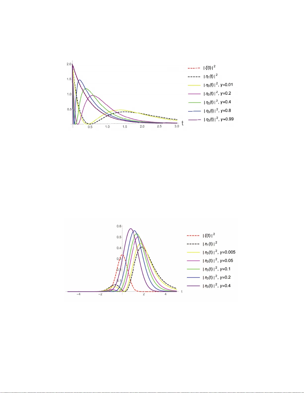
Con trol of con tin uous-mo de single-photon states: a review Guofeng Zhang ∗ July 14, 2021 Abstract In this survey , we ﬁrs t introduce quantum ﬁelds a nd op en quantum systems, then we present contin uous-mo de single-photon states a nd discuss discrete measurements of a sing le - photon ﬁeld. After that, we introduce linear quantum systems and show how a linear quantum sys tem res ponds to a single-photon input. Then we inv estigate how a coherent feedback net work can b e used to manipulate the tempo ral pulse shap e of a s ing le-photon state. Afterwards, we present single-photo n ﬁlter and master equations . Finally , we discuss the genera tion o f Schr¨ odinger cat states by means of pho ton addition and subtra ction. Keyw ords: Quan tum cont rol, con tin uous - mode singl e photon s ta tes, coheren t feedbac k, ﬁltering, master equations, Schr¨ odinger cat states . Con ten ts 1 In tro duction 2 2 Op en quantum systems 3 2.1 Field . . . . . . . . . . . . . . . . . . . . . . . . . . . . . . . . . . . . . . . . . . . 4 2.2 System . . . . . . . . . . . . . . . . . . . . . . . . . . . . . . . . . . . . . . . . . . 6 3 Con tinuous -mo de single-photon states 9 3.1 Discrete measurement of a conti nuous-mo de single-photon state . . . . . . . . . . 14 4 Linear systems’ resp onse to single-photon st a tes 16 5 Single-photon pulse shaping via coheren t feedbac k 21 6 Single-photon ﬁlter and master equation 22 ∗ Department of Applied Ma thematics, The Hong Kong Polytec hnic Universi ty , Hong Kong. Email: guofeng.zhang@polyu.edu .hk. 1 7 Sc hr¨ odinger cat states generation 27 8 Concluding remarks 31 1 In tro duction A ligh t ﬁeld is said to b e in an ℓ -photon state if it con tains exactly ℓ p hoto ns . When ℓ = 1, it is in a single-photon state. An optical or micro wa ve ph ot on, as an electromagnetic ﬁeld, has discr ete degrees of freedom like p olarization; it also has con tin uous degrees of freedom, for example a photon can b e viewed as a wa v epac k et with a contin uous sp ectral or spatial env elope. In this review, w e are in terested in con tinuous-mode single-photon states. Due to their highly gen uine quan tum nature, single- and f e w-ph ot on states h old p romising app lic ations in quant um comm u- nication, qu a ntum computation, quan tum metrology and qu an tu m simulatio ns. Recen tly , there has b een a rapidly gro wing int erest in the generation, comm unication, storage, and manipu la tion (e.g., p u lse shaping) of few-photon states. Th us , a new burgeoning and imp ortan t problem in the ﬁeld of qu a ntum engineering is: How to analyze and design quan tum dynamical systems driven b y few-photon states so as to ac hieve desirable cont rol p erformance; for example, pr odu c ing a single photon with p r e- sp eciﬁed p ulse shap e? In this review, w e inv estiga te single-photon states from a con trol-theoretic p ersp ectiv e. F o r physical imp le mentat ion of single photon generation, detection and storing, please refer to th e physic s literature [ 1 – 19 ] and references therein. In teraction b et wee n a photon (ﬂying qubit information carrier) and a t wo -lev el emitte r (sta- tionary qu bit information carrier) is f undamen tal to quantum information pro cessing and qu an - tum physics. Eﬃcien t in teraction is ac hiev ed when the inciden t ph ot on h as a well-deﬁned tem- p oral or frequency mo dal stru ctur e whic h matc hes that of the stationary qu bit. F or example, for atomic excitatio n b y a single photon, it is w ell-kno wn [ 20 – 22 ] that on r eso nan ce the optimal excitatio n b y a single photon of a rising exp onentia l pu lse s hape is ac hieved when γ = κ , where γ is the f ull wid th at h al f maxim um (FWHM) of the p hoto n wa ve pac ke t and κ is the deca y rate of the t w o-lev el atom. On the other hand, if the inciden t photon is of a Gaussian pulse shap e, the optimal ratio is 0 . 8 which is ac hiev ed when Ω = 1 . 46 κ , where Ω is the photon f requency bandwidth [ 20 , 21 , 23 – 25 ]. When a tw o-lev el atom is driven b y tw o co-propaga ting photons of Gaussian pulse sh a p e, n umerical simulat ions in [ 26 ] sho w that the m aximum excit ation proba- bilit y is around 0 . 88 attained at Ω = 2 ∗ 1 . 46 κ . Moreov er, when a t w o-lev el ato m is d riv en b y t w o coun ter-propagating iden tical photons, it is sho wn in [ 27 , 2 8 ] that the maxim um excitat ion probabilit y is attained at γ = 5 κ for rising exp onen tial pulse sh ap es, and Ω = 2 ∗ 1 . 46 κ f o r the Gaussian pulse sh apes. The rest of this article is organized as follo ws. Op en quant um s y s te ms are b rieﬂy intro d uced in Section 2 . Con tin uous-mo de single-photon stat es are p resen ted in Section 3 . The resp onse of a qu a ntum linear system to a s in gl e-photon input is discussed in Section 4 . In Section 5 it 2 is sho wn ho w to u se a linear coheren t feedbac k net wo rk to shap e the temp oral pulse of a single photon. Single-photon ﬁlters and master equations are p resen ted in Section 6 . Schr¨ odinger cat states generation is discussed in Section 7 . Tw o p ossible futu r e researc h p roblems are prop osed in Section 8 . Notation. The redu ce d Planc k constan t ~ is set to 1. | 0 i stands for th e v acuum (namely no photon) state of a free-propagating ligh t ﬁ eld. Giv en a column v ector of op erato rs or complex n umb ers X = [ x 1 , · · · , x n ] ⊤ , the Hilb ert space adjoin t op erator or complex conju g ate of X is denoted by X # = [ x ∗ 1 , · · · , x ∗ n ] ⊤ . Let X † = ( X # ) ⊤ and ˘ X = [ X ⊤ , X † ] ⊤ . The comm u ta tor b et w een operators A and B is deﬁ ned to b e [ A, B ] , AB − B A . Give n op erators L, H , X, ρ , deﬁne t wo sup erop erators Lindbladian : L G X , − i [ X , H ] + D L X, Liouvillian : L ⋆ G ρ , − i [ H , ρ ] + D ⋆ L ρ, where D L X = L † X L − 1 2 ( L † LX + X L † L ), and D ⋆ L ρ = LρL † − 1 2 ( L † Lρ + ρL † L ). ω c is th e system frequency suc h as the resonance fr equ ency of a ca vit y mo de (whic h is a quantum h arm o nic oscillato r) or th e transition frequency of a t wo-lev el sy s te m. ω o is the carr ier frequency of an external ﬁ eld. ω d = ω c − ω o is the frequency detuning. δ j k is the Kronec k er delta function and δ ( t − r ) is the Dirac delta function. The F o ur ie r trans form of a time-domain f unction ξ ∈ L 2 ( R , C ) generates ξ [ iν ] = 1 √ 2 π Z ∞ −∞ e iν t ξ ( t ) dt in the frequ e ncy domain, whose inv erse F ourier transform is ξ ( t ) = 1 √ 2 π Z ∞ −∞ e − iν t ξ [ iν ] dν. (1.1) 2 Op en quan tum systems In this section, we brieﬂy in tro duce op en quantum systems, as sho wn in Fig. 1 . In terested readers ma y refer to references [ 29 – 38 ] for mored detailed discus sio ns. Figure 1: A quan tum system G with m input ﬁelds and m output ﬁ e lds 3 2.1 Field In quantum physics, a fr e e p r opag ating Boson ﬁeld is mathematic ally mo deled b y a con tin uum of quant um h armonic oscillators, represented b y their annihilation op erators b ω and creation op erators b ∗ ω (the Hilbert space adjoin ts of b ω ). Here, ω stands for fr equencies. These ﬁ e ld op erators satisfy singular comm utation relations [ b ω , b ω ′ ] = [ b ∗ ω , b ∗ ω ′ ] = 0 , [ b ω , b ∗ ω ′ ] = δ ( ω − ω ′ ) . (2.1) Ph ysically , b ω annihilates a photon in the ﬁeld. Hence, if there is n o ph o ton in the ﬁeld, in other w ords, th e ﬁ eld is in the v acuum s tate | 0 i , then b ω | 0 i = 0. The Hamiltonian of the ﬁ el d is H B = Z ∞ 0 dω ω b † ω b ω . (2.2) By ( 2.1 ), in the Heisen b erg picture, the free ev olution of b ω is go v erned by b ω ( t ) = e iH B t b ω e − iH B t = e − iω t b ω . (2.3) Hence, H B ( t ) = Z ∞ 0 dω ω b † ω ( t ) b ω ( t ) = H B , (2.4) i.e., the Hamiltonian of a fr ee-ev olution ﬁeld is ind epend en t of time. F o r op en q u an tum s yste ms, we are in terested in the in teraction b et ween the ﬁeld and the system of interest, s ta rting from an initial time. In this p aper, we use t 0 to d en o te the initial time. After the initial time, the ﬁeld do es not ev olv e on its own du e to its in teraction with the system. As a result, ( 2.4 ) d oes not hold an y longer. Instead, the ﬁeld will carry system’s information. It is b ecause of this that the system can b e r ea d when the ﬁ eld is measur ed. Remark 2.1. A qu a ntum system has a c haracteristic frequ ency , e.g., th e atomic transition fre- quency b et w een energy lev els of an atom, the resonant fr equency of a quantum ca vit y r eso nator, or the Rabi frequency of a con tin uous-wa v e (cw) d riving laser. When the system interac ts with an input ﬁ el d (often called in ci dent ﬁeld in quant um optics), it is a standard assumption that only the ﬁ el d mod es whose frequencies are n ea r the c haracteristic frequency of th e sys tem con- tribute to the interact ion with th e system, wh il e the inﬂuence of those mo des whose frequencies are far a w a y f rom the c haracteristic frequency of the system is negligi ble. In other words, it is often the case that the eﬀe ctive ﬁ eld is within a narrow sideband cen tered at this characte ristic frequency . Under this assumption (narrow band appr o ximation), the range of inte gral of ( 2.2 ) can b e extended fr om −∞ to ∞ . More d iscussions can b e found in, e.g., [ 39 , 4 0 ]. In the inpu t- outpu t formalism of op en quantum systems, the in put ﬁeld in the time domain is deﬁned as (see e.g. [ 39 , (4 )], [ 40 , (2.14) ], [ 41 , Sec. I I I]) b in ( t ) , 1 √ 2 π Z ∞ −∞ dω e − iω ( t − t 0 ) b ω ( t 0 ) , t ≥ t 0 , (2.5) 4 where b ω ( t 0 ) denotes the quan tum harmonic oscillator b ω at the initial time t 0 . It can b e seen from ( 2.3 ) and ( 2.5 ) that b in ( t ) is a con tinuum of quan tum harmon ic oscillators b ω for all frequencies. b ∗ in ( t ), the adjoint of b in ( t ), is obtained b y conjugating b oth sides of ( 2.5 ), b ∗ in ( t ) = 1 √ 2 π Z ∞ −∞ e iω ( t − t 0 ) b ∗ ω ( t 0 ) dω , t ≥ t 0 . By ( 2.1 ), we h a ve the singular commutatio n relations for b in ( t ) and b ∗ in ( t ) in the time domain, [ b in ( t 1 ) , b in ( t 2 )] = [ b ∗ in ( t 1 ) , b ∗ in ( t 2 )] = 0 , [ b in ( t 1 ) , b ∗ in ( t 2 )] = δ ( t 1 − t 2 ) , t 1 , t 2 ≥ t 0 . (2.6) F or the input ﬁeld b in ( t ) in the time domain d eﬁned in ( 2.5 ), we d e ﬁn e its F ourier transform as b in [ iω ] , 1 √ 2 π Z ∞ t 0 dt e iω t b in ( t ) , ω ∈ R . (2.7) The adjoint b ∗ in [ iω ] of b in [ iω ] is obtained b y conju g ating b oth sid es of ( 2.7 ); sp eciﬁcall y , b ∗ in [ iω ] = 1 √ 2 π Z ∞ t 0 dt e − iω t b ∗ in ( t ) , ω ∈ R . Noticing the iden tit y lim t 0 →−∞ 1 2 π Z ∞ t 0 dt e iω t = δ ( ω ) , it can b e readily sho wn that lim t 0 →−∞ [ b in [ iω ] , b ∗ in [ iω ′ ]] = δ ( ω − ω ′ ) , ω , ω ′ ∈ R . (2.8) Remark 2.2. F or any ﬁxed t 0 , applyin g the inv ers e F ourier transform to ( 2.5 ) yields b ω ( t 0 ) e iω t 0 = 1 √ 2 π Z ∞ −∞ e iω t b in ( t ) dt, t ≥ t 0 . This, together with ( 2.3 ), giv es b ω = 1 √ 2 π Z ∞ −∞ e iω t b in ( t ) dt, t ≥ t 0 . (2.9) In the limit t 0 → −∞ , ( 2.7 ) and ( 2.9 ) yield b in [ iω ] = b ω , (2.10) whic h conﬁ rms consistency b et w een ( 2.1 ) and ( 2.8 ). Remark 2.3. In the deﬁnition of b in ( t ) in ( 2.5 ), if we implicitly assume that b in ( t ) ≡ 0 for t < t 0 , then ( 2.7 ) b ecomes b in [ iω ] = 1 √ 2 π Z ∞ −∞ dt e iω t b in ( t ) , ω ∈ R , (2.11) 5 whic h is the same as ( 2.9 ). As a result, ( 2.10 ) holds withou t taking the limit t 0 → −∞ . In deed, b y ( 2.3 ) and ( 2.5 ), w e h a ve b in ( t ) = 1 √ 2 π Z ∞ −∞ e − iω t b ω dω , t ≥ t 0 . (2.12) Th us , und er the assump ti on that b in ( t ) ≡ 0 f or t < t 0 , F ourier tr an s forming ( 2.12 ) yields ( 2.10 ), i.e., b ω = 1 √ 2 π Z ∞ −∞ dt e iω t b in ( t ) = b in [ iω ] , (2.13) where ( 2.11 ) has b een u sed. In v iew of this, it app ears meaningful to in terpret the v ariable “ t ” in ( 2.5 ) as the real time u nder the assumption that b in ( t ) ≡ 0 for t < t 0 where t 0 is the time when the system and the ﬁeld start their int eraction. This is ﬁ ne as w e are in terested in the dynamics of op en quan tum systems, instead of f r ee ev olution of th e system or the ﬁeld itself. (This int erpr et ation is diﬀeren t from that in [ 42 , Sec. 2.2].) In the s t ud y of sto c hastic Sc hr¨ od in ge r equations it is alw a ys assumed that t 0 = 0 or some ﬁn ite v alue. On the other h and, in the stud y of photon scattering oﬀ a standing emitter, it is ofte n assumed that t 0 = − ∞ , i.e. the in teractio n starts in the r emo te past. Under the treatmen t prop osed ab o ve , the s p eciﬁc v alue of th e initial time t 0 is not imp ortant. W e end this subsection as a ﬁn a l r emark. Remark 2.4. In this r evie w , we often omit the subscript “ in ” for the input ﬁelds. Thus b ( t ) is the input ﬁeld in the time domain while b [ iω ] is the input ﬁeld in the fr e que nc y doma in. Cle arly, b [ iω ] and b ω ar e diﬀer ent obje cts. However, as shown in ( 2.13 ) , they c an b e the same under some c ondition. 2.2 System The op en Marko vian quantum system G , as shown in Fig. 1 , can b e describ ed in the so-called ( S, L, H ) formalism [ 32 , 33 , 35 , 43 ]. In this formalism, S, L, H are op erators on the Hilb ert space for the system G . Sp eciﬁcally , S is a scattering op erator that satisﬁes S † S = S S † = I (the iden tit y op erator). F or example, S can b e a phase shifter or b eamsplitter, L = [ L 1 , . . . , L m ] ⊤ describ es ho w th e system G interac ts with its surroun ding environmen t, and the self-a dj o int op erator H d enote s th e inherent s y s te m Hamiltonian of G . The quantum system G is driven b y m inp ut ﬁelds. Denote the annihilation op erat or of th e j -th Boson input ﬁeld b y b j ( t ) and the creation op erator, the adjoin t op erator of b j ( t ), by b ∗ j ( t ), j = 1 , . . . , m . Then similar to ( 2.6 ), the ﬁelds satisfy the follo wing singular comm utation relations: [ b j ( t ) , b ∗ k ( r )] = δ j k δ ( t − r ) , j, k = 1 , . . . , m, and t, r ≥ t 0 . (2.14) 6 Denote a column of vect ors b ( t ) = [ b 1 ( t ) , · · · , b m ( t )] ⊤ . The integ rated input annihilation, cre- ation, and gauge pro cesses (counting pro cesses) are giv en by B ( t ) = Z t t 0 b ( s ) ds, B # ( t ) = Z t t 0 b # ( s ) ds, Λ( t ) = Z t t 0 b # ( s ) b ⊤ ( s ) ds, (2.15) resp ectiv ely . In this pap er, the inp ut ﬁelds are assumed to b e ca nonical ﬁelds whic h include the v acuum, coheren t, single- and multi-photon ﬁelds but n ot the th er m a l ﬁelds. Then these quan tum stochastic pro cesses satisfy dB j ( t ) dB ∗ k ( t ) = δ j k dt, dB j ( t ) d Λ k l ( t ) = δ j k dB l ( t ) , d Λ j k ( t ) dB ∗ l ( t ) = δ k l dB ∗ j ( t ) , d Λ j k ( t ) d Λ lm ( t ) = δ k l d Λ j m ( t ) . According to qu a ntum m echanics, th e whole system in Fig. 1 evolv es in a unitary manner. Sp eciﬁcally , th e re is a unitary op erator U ( t ) on the tensor p r odu ct System ⊗ Field Hilb ert s pace that go v erns the temp oral ev olution of this quan tum system. It tur ns out that the unitary op erator U ( t ) is the s o lution to the Itˆ o quan tum stochasti c diﬀeren tial equation (QSDE) dU ( t ) = ( −  iH + 1 2 L † L  dt + LdB † ( t ) − L † S dB ( t ) + T r[ S − I ] d Λ( t ) ) U ( t ) (2.16) with the initial cond it ion U ( t 0 ) = I . I n particular, if L = 0 and S = I , then ( 2.16 ) r ed uces to i ˙ U = H U, whic h is the Sc hr ¨ odinger equation for an isolated qu an tum system w ith Hamilto nian H . Using the u nitary op erator U ( t ) in ( 2.16 ), the dynamical ev olution of system op erators and the environmen t can b e obtained in the Heisenber g p ictur e . Indeed, the time ev olution of the system op erator X , denoted by j t ( X ) ≡ X ( t ) = U † ( t )( X ⊗ I ﬁeld ) U ( t ) , (2.17) follo ws the Itˆ o QSDE d j t ( X ) = j t ( L G X ) dt + dB † ( t ) j t ( S † [ X, L ]) + j t ([ L † , X ] S ) dB ( t ) +T r[ j t ( S † X S − X ) d Λ( t )] . On the other hand, the d ynamica l ev olution of the output ﬁeld is given b y dB out ( t ) = L ( t ) dt + S ( t ) dB ( t ) , d Λ out ( t ) = L # ( t ) L ⊤ ( t ) dt + S # ( t ) dB # ( t ) L ⊤ ( t ) + L # ( t ) dB ⊤ ( t ) S ⊤ ( t ) + S # ( t ) d Λ( t ) S ⊤ ( t ) , 7 where B out ( t ) = U † ( t )( I system ⊗ B ( t )) U ( t ) , Λ out ( t ) = U † ( t )( I system ⊗ Λ( t )) U ( t ) are the integ rated output ann ihila tion op erat or and gauge pro cesses, resp ectiv ely . Example 2.1 (O p tic al cavit y) . Let G b e an optical ca vit y . Here w e consider the simplest case: the ca vity has a sin g le in traca vit y mo de (a quan tum harmonic oscillator represen ted b y its annih il ation op erator a ) whic h int eracts with an external ligh t ﬁeld represente d b y its annihilation op erat or b ( t ). Because a is a ca vit y mo de, it and its adjoin t op erator a ∗ satisfy the canonical commuta tion relation [ a, a ∗ ]=1, in contrast to the singular comm utation relation ( 2.14 ) for free propagating ﬁelds. As in tro duced in th e Notation part, let ω d b e the detuned frequency b et w een the resonance frequency of the int ernal mo de a and the cen tral fr equ ency of the external ligh t ﬁeld b ( t ). Let κ b e th e half linewidth of the ca vit y . I n the ( S, L, H ) formalism, w e h av e S = I , L = √ κa , and H = ω d a ∗ a . Then, the dynamics of this line ar sy s te m can b e describ ed in the inpu t -outpu t form da ( t ) = − ( iω d + κ 2 ) a ( t ) dt − √ κdB ( t ) , (2.18) dB out ( t ) = √ κa ( t ) dt + dB ( t ) . Applying the Laplace transform to ( 2.18 ) and omitting the inﬂu ence of the initial state a ( t 0 ) yield a [ iω ] = − √ κ i ( ω + ω d ) + κ 2 b [ iω ] = − T [ iω ] b [ iω ] , where T [ iω ] , √ κ i ( ω + ω d ) + κ 2 (2.19) is called the amplitude tr ansmission function in optics literature; s ee e.g., [ 44 ]. T [ iω ] giv es the relation b et w een the intra- ca vit y mod e and the input mo de and is in the form of a Loren tzian lineshap e function; see ( 3.6 ). Finally , the v alue T [0 ] = √ κ iω d + κ 2 in the neigh b orho od of the resonance of the ca vit y is commonly u sed in optics. Example 2.2 (Tw o-lev el s y s te m) . A t wo- lev el system r esiding in a c hiral nanophotonic w a ve g- uide can b e parametrized b y the triple S = 1, L = √ κσ − , and H = ω d 2 σ z . The t w o-lev el system has t wo energy state s: the ground state | g i and excited state | e i . σ − = | g i h e | and σ + = | e i h g | are the low ering and raising op erato r resp ectiv ely . W e hav e σ − | g i = 0 and σ + | e i = 0. σ z = | e i h e | − | g i h g | is the P auli Z op erator. Th e scalar ω d is the detuning fre- quency b et w een the transition f r equency (b et w een | g i and | e i ) of the tw o-lev el system and the 8 cen tral frequency of the external ligh t ﬁeld, and κ is the deca y rate of the t w o-lev el system. The dynamics of the system are describ ed by dσ − ( t ) = − ( iω d + κ 2 ) σ − ( t ) dt + √ κσ z ( t ) dB ( t ) , dB out ( t ) = √ κσ − ( t ) dt + dB ( t ) . It sh ou ld b e n oted that this system is biline ar du e to the p resence of σ z ( t ) dB ( t ), in con trast to the linear r eso nator in Example 2.1 . Ho w eve r, if the tw o-lev el atom is initially in th e ground state | g i and th e ﬁeld is in the v acuu m s t ate | 0 i , as σ z ( t ) | g 0 i = − | g 0 i (see e.g., [ 22 , Lemma 3]), w e h a ve dσ − ( t ) | g 0 i = − ( iω d + κ 2 ) σ − ( t ) dt | g 0 i − √ κdB ( t ) | g 0 i , dB out ( t ) | g 0 i = √ κσ − ( t ) | g 0 i dt + dB ( t ) | g 0 i , whic h is in the form of line ar dynamics. Finally , rotations σ − ( t ) → e i ω d t σ − ( t ) , B ( t ) → e i ω d t B ( t ) , B out ( t ) → e i ω d t B out ( t ) put the ab o ve system int o the follo wing form dσ − ( t ) | g 0 i = − κ 2 σ − ( t ) dt | g 0 i − √ κdB ( t ) | g 0 i , dB out ( t ) | g 0 i = √ κσ − ( t ) | g 0 i dt + dB ( t ) | g 0 i . Remark 2.5. In th is section, the d ynamics of a qu an tum system are giv en d irec tly in terms of the sys tem op erato rs S, L, H . This is un li ke the traditional w a y where the starting p oin t is a total Hamiltonian for the join t system-ﬁeld system, see, e.g, [ 39 ]. Nev ertheless, the ( S, L , H ) formalism originates f rom and is a simpliﬁed ve rsion of the traditional appr oa c h [ 32 ]. An illustrative example can b e f o un d in [ 26 , Example 1]. 3 Con tin u ou s- mod e single-photon states In this s ection, w e introdu ce single-photon states of a free p r opag ating light ﬁeld. Denote | 1 t i = b ∗ ( t ) | 0 i . By ( 2.14 ) and b ( t ) | 0 i = 0, we hav e h 1 t | 1 τ i = δ ( t − τ ). A contin uous- mo de single-photon state of a ligh t ﬁeld having the temp oral pu lse shap e ξ ( t ) ∈ L 2 ( R , C ) can b e viewed as a su perp osition of the contin uum of | 1 t i ; in other w ords, | 1 ξ i ≡ B ∗ ( ξ ) | 0 i , Z ∞ −∞ ξ ( t ) | 1 t i dt. (3.1) Assume the L 2 norm k ξ k , q R ∞ −∞ | ξ ( t ) | 2 dt = 1. (It is assumed that ξ ( t ) ≡ 0 for t < t 0 (the initial time) as we fo cus on the in teraction b et ween a system and a ﬁeld.) Then h 1 ξ | 1 ξ i = 1. 9 Hence, the probabilit y of ﬁnd ing the p h ot on in th e time interv al [ t, t + dt ) is | ξ ( t ) | 2 dt . In the frequency domain, we use | 1 ω i , b ∗ [ iω ] | 0 i . In the fr equency domain ( 3.1 ) b ecomes | 1 ξ i = Z ∞ −∞ ξ [ iω ] | 1 ω i dω . (3.2) Remark 3.1. If we do not restrict ξ to b e in L 2 ( R , C ), for example, let ξ [ iω ] = δ ( ω − ω 0 ) for some r ea l ω 0 ; in other w ords, we ha v e a mono c h romati c ligh t ﬁ eld w it h fr equency ω 0 . Then from ( 3.2 ) we get | 1 ξ i = b ∗ [ iω 0 ] | 0 i = | 1 ω 0 i . Moreo v er, by ( 1.1 ) we get the temporal wa ve pac k et ξ ( t ) = 1 √ 2 π e iω 0 t whose mo dulus is | ξ ( t ) | ≡ 1 √ 2 π for all t ∈ R . If a ﬁ eld is r estricted to b e in the in terv al [ t 0 , t ], ( 3.1 ) b ecomes | 1 ξ i = Z t t 0 ξ ( r ) | 1 r i dr. Similarly , an ℓ -photon state of a ﬁeld ov er the interv al [ t 0 , t ] can b e deﬁn ed as | ℓ ψ i = Z t t 0 · · · Z t t 0 ψ ( τ 1 , . . . , τ ℓ ) | 1 τ 1 i · · · | 1 τ ℓ i dτ 1 · · · dτ ℓ . (3.3) In other words, by means of a con tinuum of basis ve ctors {| 0 i , | 1 τ 1 i , · · · , | 1 τ ℓ i : τ 1 , . . . , τ ℓ ∈ [ t 0 , t ] } , an y ℓ -photon state can b e expr essed in the w a y giv en in ( 3.3 ). As photons are indistin- guishable, the f u nctio n ψ in ( 3.3 ) is p erm utation-in v arian t w.r.t. τ 1 , . . . , τ ℓ . Under the single-photon state | 1 ξ i , the ﬁ eld op erator b ( t ), w hic h is a quantum sto c hastic pro cess, h a s zero mean, and w hose co v ariance f unction is R ( t, r ) , h 1 ξ | ˘ b ( t ) ˘ b † ( r ) | 1 ξ i = δ ( t − r ) " 1 0 0 0 # + " ξ ( r ) ∗ ξ ( t ) 0 0 ξ ( r ) ξ ( t ) ∗ # , t, r ≥ t 0 . By ( 2.15 ), th e gauge pro cess is Λ( t ) = R t t 0 n ( r ) dr , where n ( t ) , b ∗ ( t ) b ( t ) is the num b er op erator f o r th e ﬁeld. In the case of th e single-photon state | 1 ξ i deﬁned in ( 3.1 ), the intensit y is the mean ¯ n ( t ) , h 1 ξ | n ( t ) | 1 ξ i = | ξ ( t ) | 2 . Clearly , R ∞ t 0 ¯ n ( t ) dt = 1, i.e., there is one ph ot on in th e ﬁeld. Next, w e lo ok at thr ee commonly used single-photon states. Firstly , when ξ ( t ) is an exp o- nen tially deca ying pulse s hape ξ ( t ) = ( √ β e − ( β 2 − iω o ) t , t ≥ 0 , 0 , t < 0 , (3.4) 10 the state | 1 ξ i can describ e a single photon emitted f rom an optical ca vit y with resonan t frequency ω o and damping rate β or a t wo -lev el atom with ato mic transition f requency ω o and deca y rate β [ 45 , 46 ]. The fr equ ency count erp art of ( 3.4 ) is ξ [ iω ] = r β 2 π 1 β 2 + i ( ω − ω o ) . Secondly , if ξ ( t ) is a rising exp onen tial p ulse shap e ξ ( t ) = ( √ β e ( β 2 + iω o ) t , t ≤ 0 , 0 , t > 0 , (3.5) in the frequ e ncy represen tation it is ξ [ iω ] = r β 2 π 1 β 2 − i ( ω − ω o ) . (3.6) where ω o is th e carrier frequency of the light ﬁeld, then on resonance the single-photon s ta te | 1 ξ i is able to fully excite a t w o-lev el system if β = κ , where κ is the deca y rate as in tro duced in Example 2.2 , see, e.g., [ 20 – 22 , 47 ]. The sin g le photon with pulse shap e ( 3.4 ) or ( 3.5 ) has Loren tzian lineshap e function with the full width at half maxim um (FWHM) β [ 46 , 48 ], which in the fr e que nc y domain satisﬁes | ξ [ iω ] | 2 = 1 2 π β ( ω − ω o ) 2 +  β 2  2 , whic h is [ 40 , (3.28)] with F = 1 (the single-photon case). Finally , the Gaussian pulse shap e can b e giv en by ξ ( t ) =  Ω 2 2 π  1 4 exp  − Ω 2 4 ( t − τ ) 2  , (3.7) where τ is the ph ot on p eak arriv al time. Applying F ourier transform to ξ ( t ) in ( 3.7 ) we get | ξ [ iω ] | 2 = 1 √ 2 π (Ω / 2) exp  − ω 2 2(Ω / 2) 2  . Hence, Ω is the frequency ban d width of the single-photon wa vepac ket . Actuall y , ξ [ iω ] = 1 ( π 2 Ω 2 ) 1 / 4 exp  ω ( iτ − ω Ω 2 ))  = 1 ( π 2 Ω 2 ) 1 / 4 exp −  ω − iπ Ω / 2 Ω  2 −  τ Ω 2  2 ! . 11 Let τ = 0 and Ω = √ 2 R . Then (3.8) b ecomes ξ [ iω ] = 1 π 1 / 4 √ R exp  − ( ω /R ) 2 2  . (3.8) Similarly , ( 3.7 ) b ecomes ξ ( t ) = √ R π 1 / 4 exp  − ( Rt ) 2 2  . (3.9) ( 3.8 )-( 3.9 ) are th e form of the wa vefunction of a v acuum state [ 29 , Chapter 4]. In particular, if R 6 = 1, ( 3.8 )-( 3.9 ) are in th e form of the wa vefunction of a squeezed v acuum s tate [ 49 , Eqs. (5.3)- (5.4)]. Th is is not s urprising b eca use v acuum states and squeezed v acuum states are coherent states whic h ha ve Gaussian w a v e-pac ke ts. In con trast to the full excitatio n of a t wo-l eve l atom by a sin gl e photon of rising exp onen tial pulse shap e ( 3.5 ), th e maximal excitatio n probabilit y of a t w o-lev el atom b y a single ph ot on of Gaussian pulse sh ap e ( 3.7 ) is around 0.8 which is achiev ed at Ω = 1 . 46 κ , see, e.g., [ 20 – 22 , 26 , 47 ]. F or a mathematical theory of ho w to generate a sin gl e-photon of a p rescribed temp oral pulse, int erested readers ma y refer to [ 50 ]. F or physical generatio n of a sin g le photon of rising exp onen tial pulse sh ape, intereste d readers may r e fer to [ 14 , 44 ]. Remark 3.2. It should b e noted that a con tinuous-mod e single-photon state | 1 ξ i discussed ab o v e is diﬀerent from a con tin uous -mo de single-photon c oher ent state | α ξ i which can b e d eﬁ ned as | α ξ i , exp( α B ∗ ( ξ ) − α ∗ B ( ξ )) | 0 i , (3.10) where α = e iθ ∈ C . F or | α ξ i , although the mean photon num b er is h α ξ | B ∗ ( ξ ) B ( ξ ) | α ξ i = | α | 2 = 1 , whic h is the same as the single-photon state | 1 ξ i , the mean amplitud e is h α ξ | B ( ξ ) | α ξ i = α . In contrast, the mean amplitud e of the s ingle -photon state | 1 ξ i is h 1 ξ | B ( ξ ) | 1 ξ i = 0. More discussions can b e found in [ 51 , S ec tion 2.1], [ 35 , Section 7.1.1 ]. Finally , con tin uum coheren t states are d eﬁ ned in [ 40 , (3.1) and (3.6)] and [ 21 , (24)], whic h in our notation are of the f orm |{ α [ iω ] }i = exp  Z ∞ −∞ dω ( α [ iω ] b [ iω ] † − α [ iω ] ∗ b [ iω ])  | 0 i . (3.11) Clearly , if α [ iω ] = αξ [ iω ], ( 3.11 ) b ecomes ( 3.10 ). A time-domain discu s sio n can b e found in [ 47 ]. If an electromagnetic ﬁeld is conﬁned for example in a ca vit y , it will ha v e discrete mod es instead of a con tin uum of mo des. Next, w e int ro duce single-mo de coheren t states. If a laser is inciden t on the cavit y , the cavit y can b e in a coherent s tate. Moreo ver, in quantum optics, laser is often assumed to pro duce a single-mo de coheren t signal. The reason is simple, if the p ulse 12 ξ [ iω ] ≡ γ δ [ ω o ] in ( 3.10 ) , where γ ∈ R and ω o is the central fr equency , then we ha ve a single-mo de coheren t state | β i = exp( β b ∗ [ iω o ] − β ∗ b [ iω o ]) | 0 i , (3.12) where β = αγ ∈ C . Th e single-mo de coheren t state | β i can b e rewritten as | β i = e − 1 2 | β | 2 ∞ X n =0 β n √ n ! | n i . (3.13) Clearly , the v acuum s ta te | 0 i is a coherent state ( β = 0 in ( 3.12 )). Another t yp e of single-mo de coheren t states, single-mo de squeezed v acuum states, will b e introd uced in Section 7 . Finally , it is worth while to p oin t out that there is a slight abu s e of notation in ( 3.12 ). In this sur v ey , the annihilation op erator of a f ree propagating ﬁ eld is denoted by b ( t ), wh il e that f o r a ca vit y is denoted by a ( t ). Ho wev er, as we w ant to sho w that the single-mo de coheren t state | β i in ( 3.12 ) is an ideal app ro xim ation of the cont inuous-mod e coheren t s ta te | α ξ i in ( 3.10 ), we feel it is go o d to use b ( t ) in b oth of these tw o equations. More discussions on coheren t states can b e f o un d in [ 29 , Chapter 4]. Remark 3.3. The op erato r B ∗ ( ξ ) deﬁned via ( 3.1 ) is called a discrete p hoto n creation op erator in the temp oral mo des theory of qu an tum optics; see e.g., [ 52 , (2.14)] and [ 53 , (7)]. Roughly sp eaking, un der th e narr ow-b and appr oximation as describ ed in Remark 2.1 , using b [ iω ] we can deﬁne a time-spatial op erator, [ 45 , (7.3)], b ( x, t ) = e − iω o ( t − x/c ) 1 √ 2 π Z ∞ −∞ dω ′ b [ iω ′ ] e − iω ′ ( t − x/c ) , where ω o is the carrier frequency of th e free propagating ﬁeld. Denote E + ( x, t ) = ib ( x, t ) , (3.14) E − ( x, t ) = − ib ( x, t ) ∗ = ( E + ( x, t )) ∗ . Then in a simpliﬁ ed form, an electromagnetic ﬁeld propagating along the p ositiv e x d ir ec tion can b e describ ed as, [ 54 ], E ( x, t ) = E + ( x, t ) + E − ( x, t ) = i ( b ( x, t ) − b ( x, t ) ∗ ) . Let { ξ j } b e an orthonormal basis of the sp ac e of th e square-inte grable pulse shap es ξ . An example of { ξ j [ iω ] } is the set of wight ed Hermite p olynomials [ 55 , Chapter 8]. Deﬁne B j , B ( ξ j ) = Z ∞ −∞ dt b ( t ) ξ ∗ j ( t ) = Z ∞ −∞ dω b [ iω ] ξ ∗ j [ iω ] . Clearly , B ∗ j | 0 i generates a ph ot on of pu lse shap e ξ j . Moreo ve r, as { ξ j } is an orthonormal basis, w e h a ve X j ξ j [ iω ] B j = Z ∞ −∞ dω ′ b [ iω ′ ] X j ξ j [ iω ] ξ ∗ j [ iω ′ ] Z ∞ −∞ dω ′ b [ iω ′ ] δ ( ω − ω ′ ) = b [ iω ] . (3.15) 13 Deﬁne a time-spatial function ν j ( x, t ) whic h is associated with ξ j b y ν j ( x, t ) , ie − iω o ( t − x/c ) 1 √ 2 π Z ∞ −∞ dω ′ ξ j [ iω ′ ] e − iω ′ ( t − x/c ) . (3.16) By ( 3.15 )-( 3.16 ), the p ositiv e-frequency part E + ( x, t ) of an electromagnetic ﬁ el d deﬁned in ( 3.14 ) can b e re-written as E + ( x, t ) = X j ν j ( x, t ) B j . More discussions can b e foun d in a recen t review on temp oral m odes in quan tum optics [ 53 ]. 3.1 Discrete measuremen t of a contin uous-mo de single-photon state In this subsection, w e present a pro cedure of digitizing a contin uous-mo de single-photon state | 1 ξ i as is p roposed in [ 44 ]. Assume that the time in terv al ( −∞ , ∞ ) is partitioned into time bins of equal length ∆ t and let t j = j ∆ t for j = 0 , ± 1 , . . . . When ∆ t is s uﬃcien tly small, th e v alue of ξ ( t ) in th e time bin [ j ∆ t, ( j + 1)∆ t ) is well app ro ximated by ξ t j . Then a con tin uous-mo de single-photon state | 1 ξ i can b e appro ximately written as | 1 ξ i = Z ∞ −∞ ξ ∗ ( t ) b ∗ ( t ) dt | 0 i = X j ξ ∗ ( t j ) 1 ∆ t Z t j +1 t j b ∗ ( t ) dt | 0 i . (3.17) Denote | 1 j i = c ∗ j | 0 i ≡ 1 ∆ t Z t j +1 t j b ∗ ( t ) dt | 0 i . (3.18) Notice that [ c j , c ∗ k ] = δ j k ∆ t . (3.19) Remark 3.4. According to ( 3.19 ), [ c j , c ∗ j ] b ec omes a Dirac delta function δ ( t j ) in the limit ∆ t → 0. This justiﬁes the co eﬃcien t 1 ∆ t in the deﬁn iti on of c ∗ j in ( 3.18 ). By means of ( 3.18 ), the app ro ximated single-photon state in ( 3.17 ) can b e re-wr it ten as | 1 ξ i = X j ξ ∗ ( t j ) | 1 j i . The corresp onding density matrix is ρ = | 1 ξ i h 1 ξ | = X mn ρ mn | 1 m i h 1 n | , (3.20) where ρ mn = ξ ∗ ( t m ) ξ ( t n ). Deﬁne a quadrature X j for the j th time bin to b e X j , c j e − iθ j + c ∗ j e iθ j √ 2 (3.21) 14 where θ j = ω d · t j + θ 0 with ω d b eing the frequency d etuning b et w een the cen tral frequen c y of the signal (the single- photon stat e | 1 ξ i ) an d that of the local oscilla tor for homo dyne measuremen t, and θ 0 b eing the lo cal oscillator’s relativ e ph ase at t = 0. As X j = X ∗ j , X j is an observ able whic h can b e measured in principle. Moreo v er, it can b e sh own that [ X j , X k ] = − iδ j k ∆ t sin(( j − k ) ω d ∆ t ) = 0 , j 6 = k . The time s er ies { X j } can b e measured in exp eriments. Remark 3.5. Notice that the quad r at ur e X j deﬁned in ( 3.21 ) can b e re-written as X j = c j + c ∗ j √ 2 cos θ j + c j − c ∗ j i √ 2 sin θ j ≡ Q j cos θ j + P j sin θ j , where the qu ad r at ur es Q j = c j + c ∗ j √ 2 and P j = c j − c ∗ j i √ 2 satisfy [ Q j , P j ] = i ∆ t . It can b e calculated that X k | 1 m i = e − iθ k √ 2 δ k m | 0 i + 1 ∆ t e iθ k √ 2 Z t j +1 t j dt Z t m +1 t m dr b ∗ ( t ) b ∗ ( r ) | 0 i . (3.22) Therefore, we h av e h 1 n | X j X k | 1 m i = 1 2 ( e − i ( θ k − θ j ) δ k m δ j n + δ j k δ mn + e − i ( θ j − θ k ) δ j m δ k n ) . (3.23) Let I ( t j ) b e the homo dyne current for the j th time bin, which is prop ortional to X j . By ( 3.20 ) and ( 3.23 ), we hav e h I ( t j ) I ( t k ) i ∝ h X j X k i = T r [ ρX j X k ] = X mn ρ mn h 1 n | X j X k | 1 m i = 1 2 ( e − i ( θ k − θ j ) ρ k j + δ j k + e − i ( θ j − θ k ) ρ j k ) = 1 2 δ j k + Re[ ρ j k ] cos( θ j − θ k ) + Im[ ρ j k ] sin( θ j − θ k ) = 1 2 δ j k + Re[ ρ j k ] cos( ω d ( t j − t k )) + Im[ ρ j k ] sin( ω d ( t j − t k )) , whic h is [ 44 , (5)]. Remark 3.6. In an exp eriment , it is the homod yne photo curren t I ( t ) th a t is recorded, from whic h h X j X k i is obtained b y a v eraging o ver many tra jectories. After getting h X j X k i , Re[ ρ j k ] and Im[ ρ j k ] can b e retriev ed, from which we can get a discrete approxima tion of ξ ( t ). 15 4 Linear systems’ resp onse to single-photon states Let the system G in Fig. 1 b e linear and d r iv en by m ph ot ons, one in eac h input ﬁeld. Also, assume that G is initialized in a coherent state . Single-mo de coherent stat es are deﬁn ed in ( 3.13 ), its multi-mode count erpart can b e found in [ 56 , Section I I-E]. In this section, we presen t the state of the output ﬁelds. Giv en tw o constant matrices U , V ∈ C r × k , a doub led-up matrix ∆ ( U, V ) is deﬁned as ∆ ( U, V ) , " U V V # U # # . Let I k b e an iden tit y matrix and 0 k a zero square matrix, b oth of dimension k . Deﬁne J k = diag( I k , − I k ). T hen for a matrix X ∈ C 2 j × 2 k , deﬁne X ♭ = J k X † J j . In the linear case, the system G can b e used to mo del a collect ion of n quan tum harmonic oscillators that are drive n b y m inpu t ﬁelds. Denote a ( t ) = [ a 1 ( t ) · · · a n ( t )] ⊤ , where a j ( t ) is the annihilation op erator for the j th harmonic oscillator, j = 1 , . . . , n . I n the ( S, L , H ) formalism, the inh er ent system Hamiltonian is giv en by H = (1 / 2)˘ a † Ω˘ a , where a = [ a ⊤ ( a # ) ⊤ ] ⊤ , and Ω = ∆(Ω − , Ω + ) ∈ C 2 n × 2 n is a Hermitian matrix with Ω − , Ω + ∈ C n × n . The coup li ng b et w een the sys tem and the ﬁelds is describ ed by the op erator L = [ C − C + ]˘ a , with C − , C + ∈ C m × n . Finally , th e scattering op erator S is an m × m constant matrix such that S † S = S S † = I m . Th e dynamics of the op en quant um linear system in Fig. 1 are describ ed by the follo wing lin e ar Itˆ o QSDEs ( [ 57 , (26)], [ 56 , (14)- (15)], [ 38 , (5)-(6)], [ 58 , 59 ], [ 37 , C h apter 2]), d ˘ a ( t ) = Aa ( t ) dt + B d ˘ B ( t ) , d ˘ B out ( t ) = C a ( t ) dt + D d ˘ B ( t ) , t ≥ t 0 , (4.1) where D = ∆ ( S, 0) , C = ∆ ( C − , C + ) , B = − C ♭ ∆ ( S, 0) , A = − 1 2 C ♭ C − iJ n ∆ (Ω − , Ω + ) . These constant system m a trices are parametrized b y the physica l parameters Ω − , Ω + , C − , C + and satisfy A + A ♭ + B B ♭ = 0 , (4.2a) B = − C ♭ ∆ ( S , 0) . (4.2b) ( 4.2a ) is equiv alen t to [˘ a ( t ) , ˘ a † ( t )] ≡ [˘ a ( t 0 ) , ˘ a † ( t 0 )] = J n , ∀ t ≥ t 0 . That is, the system v ariables preserve canonical comm utation r e lations. On the other hand, ( 4.2b ) is equiv alen t to [˘ a ( t ) , ˘ b † out ( r )] = 0 , t ≥ r ≥ t 0 . 16 That is, the system v ariables and th e output s atisfy the non-demolition condition. In the quan tum control literature, equations ( 4.2a )-( 4.2b ) are called physic al r e alization conditions. Roughly sp eaking, if these conditions are m e t, the mathematical mod el ( 4.1 ) could in principle b e p h ysically realized ( [ 60 ], [ 61 ]). Let X b e an op erator on the join t system-ﬁeld sp ac e. Denote b y h X ( t ) i the exp ected v alue of X ( t ) with r espect to the initial joint s yste m-ﬁeld state. T hen ( 4.1 ) has a corresp ondin g classic al linear system of the form d h ˘ a ( t ) i = A h a ( t ) i dt + B d h ˘ B ( t ) i , d h ˘ B out ( t ) i = C h a ( t ) i dt + D d h ˘ B ( t ) i , t ≥ t 0 , (4.3) By means of the classic al linear systems theory , we can deﬁne Hur w it z stabilit y , con trollabilit y and observ abilit y of a linear quantum s y s te m. Deﬁnition 4.1. [ 34 , Deﬁnition 1] The quantum line ar system ( 4.1 ) i s said to b e H urw itz stable (r esp. c ontr ol lable, observable) if the c orr esp onding classic al line ar system ( 4.3 ) is Hurwitz stable (r esp. c ontr ol lable, observable). Moreo v er, as in classical linear systems th e ory , the impulse r esp onse function for the s yste m G is deﬁ ned as g G ( t ) , ( δ ( t ) D − C e At C ♭ D , t ≥ 0 , 0 , t < 0 . (4.4) It is easy to sho w th a t g G ( t ) deﬁned in ( 4.4 ) has th e follo win g nice stru ct ur e g G ( t ) = ∆ ( g G − ( t ) , g G + ( t )) , where g G − ( t ) ,      δ ( t ) S − [ C − C + ] e At " C † − − C † + # S, t ≥ 0 0 , t < 0 , g G + ( t ) ,      − [ C − C + ] e At " − C T + C T − # , t ≥ 0 0 , t < 0 . Giv en a function f ( t ) in the time domain, its t wo -sided Laplace transf o rm [ 62 , Chapter 10] is deﬁned as F [ s ] ≡ L b { f ( t ) } ( s ) , Z ∞ −∞ e − st f ( t ) dt. Applying the tw o-sided Laplace transform to the impu lse resp onse fu n cti on ( 4.4 ) yields the transfer fu n cti on Ξ G [ s ] = ∆(Ξ G − [ s ] , Ξ G + [ s ]) , 17 where Ξ G − [ s ] = L b { g G − ( t ) } ( s ) and Ξ G + [ s ] = L b { g G + ( t ) } ( s ). If C + = 0 and Ω + = 0, the resulting qu a ntum linear system is said to b e p assive [ 34 , 38 , 58 ]. Sp eciﬁcally , the Itˆ o QSDEs for a passiv e linear quant um system are (e.g., see [ 34 , Sec. 3.1]), da ( t ) = A a ( t ) dt + B dB ( t ) , dB out ( t ) = C a ( t ) dt + D dB ( t ) , t ≥ t 0 , (4.5) where A = − i Ω − − 1 2 C † − C − , B = − C † − S, C = C − , D = S. An equiv alen t w a y to c haracterize th e structure of the p assiv e linear quantum sys te m ( 4.5 ) is b y the physic al realiz abilit y conditions A + A † + B B † = 0 , B = −C † S. Moreo v er, in the p assive case, Ξ G + [ s ] ≡ 0 and Ξ G − [ s ] = S − C − ( sI + i Ω − + 1 2 C † − C − ) − 1 C † − S. Hence, if a linear system is passiv e, then its dyn amic s are complete ly c haracterized by its ann i- hilation op erators. Moreo ver, it can b e easily v eriﬁed th a t Ξ G − [ iω ] † Ξ G − [ iω ] ≡ I m , ∀ ω ∈ R . Hence, an empt y ca vit y do es not c hange the amplitude of the input signal, but mod iﬁ es its phase. Example 4.1 (Re-visit Example 2.1 ) . F or the c avity mo del in Example 2.1 , cle arly C + = 0 , Ω + = 0 and S = 1 . In this c ase Ξ G + [ s ] ≡ 0 and Ξ G − [ s ] = s + iω d − κ 2 s + iω d + κ 2 . As a r esult, the input-output r elation in the fr e quency domain is b out [ s ] = s + iω d − κ 2 s + iω d + κ 2 b in [ s ] . Let the linear q u an tum system G b e initialize d in the coherent state | η i and the inpu t ﬁeld b e initialized in the v acuum state | 0 i . Then the initial joint system-ﬁeld state is ρ 0 g , | η i h η | ⊗ | 0 i h 0 | in the form of a den s it y m a trix. Denote ρ ∞ g = lim t →∞ ,t 0 →−∞ U ( t, t 0 ) ρ 0 g U ( t, t 0 ) ∗ . 18 Here, t 0 → −∞ in dica tes that the in teraction starts in the remote past and t → ∞ m e ans that w e are inte rested in the dynamics in the far future. In other words, we lo ok at the steady-state dynamics. Deﬁn e ρ ﬁeld , g , h η | ρ ∞ g | η i . (4.6) In other w ords, the system is traced oﬀ and we f o cus on the steady-state s t ate of the output ﬁeld. The follo wing result giv es the resp onse of a quantum lin ear system to a sin gl e-c hannel single- photon state. Theorem 4.1. [ 56 , Pr op osition 2] Assume ther e is one input ﬁeld which i s in the sing le photon state | 1 ξ i . A lso, assume that G i s H urwitz stable and is initialize d in a c oher ent state | η i . Then the ste ady-state output ﬁeld state for the line ar quantum system G is ρ out = ( B ∗ ( ξ − out ) − B ( ξ + out )) ρ ﬁeld , g ( B ∗ ( ξ − out ) − B ( ξ + out )) ∗ , wher e ∆( ξ − out [ s ] , ξ + out [ s ]) = Ξ G [ s ]∆( ξ [ s ] , 0) , and ρ ﬁeld , g , deﬁne d in ( 4.6 ), is the density op er ator for the output ﬁeld with zer o me an and c ovarianc e function R out [ iω ] = Ξ G [ iω ] R in [ iω ]Ξ G [ iω ] † with R in [ iω ] = " 1 0 0 0 # . In p articular, if the line ar system G is p assive and initialize d in the vacuum state, then ξ + out [ s ] ≡ 0 and R out [ iω ] ≡ R in [ iω ] . In other wor ds, the ste ady-state output is a single-photon state | 1 ξ − out i . Example 4.2. L et the optic al c avity intr o duc e d in Example 2.1 b e initialize d in the vacuum state. Then, by The or em 4.1 , the ste ady-state output ﬁeld state is also a single-photon state | 1 ξ − out i with the pulse shap e ξ − out [ iω ] = i ( ω + ω d ) − κ 2 i ( ω + ω d ) + κ 2 ξ [ iω ] . Remark 4.1. It has b een sh o wn in [ 22 ] that the outpu t ﬁeld of a t w o-lev el atom initialized in the ground state and driv en by a single-photon ﬁeld | 1 ξ i is also a single-photon state | 1 ξ − out i . Th us, although the dynamics of a t wo- lev el atom is bilinear, see Example 2.2 , in the single-photon input case it can b e f ully charac terized by a linear systems theory . If the linear system G is not passive, or is not initialized in the v acuu m state, the steady- state output ﬁeld state ρ out in general is not a single-photon state; as can b e seen in Theorem 19 4.1 . Th is new typ e of states h as b een named “photon-Gaussian” states in [ 56 ]. Moreo ver, it h a s b een pro v ed in [ 56 ] that the class of “photon-Gaussian” states is in v arian t under the s teady-state action of a linear quantum sys tem. In what follo ws we p r esen t this r esult. Deﬁnition 4.2. [ 5 6 , Deﬁnition 1] A state ρ ξ ,R is said to b e a p hoton-Ga ussian state if it b elongs to the set F ,    ρ ξ ,R = m Y k =1 m X j =1  B ∗ j ( ξ − j k ) − B j ( ξ + j k )  ρ R   m Y k =1 m X j =1  B ∗ j ( ξ − j k ) − B j ( ξ + j k )    ∗ : function ξ = ∆( ξ − , ξ + ) and densit y matrix ρ R satisfy T r[ ρ ξ ,R ] = 1  . Theorem 4.2. [ 56 , The or em 5] L et ρ ξ in ,R in ∈ F b e a photon-Gaussian input state. Also, assume that G is Hurwitz stable and is initialize d in a c oher ent state | η i . Then the line ar quantum system G pr o duc es in ste ady state a photo n-Gaussian output state ρ ξ out ,R out ∈ F , wher e ξ out [ s ] = Ξ G [ s ] ξ in [ s ] , R out [ iω ] = Ξ G [ iω ] R in [ iω ]Ξ G [ iω ] † . Next, we pr e sent a result f o r the p a ssive case, which is a sp ecial case of Theorem 4.2 . Let the k th input c hannel b e in a single photon state | 1 µ k i , k = 1 , . . . , m . Th us, the state of the m -c hannel input is give n by the tensor pro duct | Ψ µ i = | 1 µ 1 i ⊗ · · · ⊗ | 1 µ m i . (4.7) Denote µ = [ µ 1 · · · µ m ] ⊤ . Corollary 4.1. Assume that the p assive line ar quantum system ( 4.5 ) is Hurwitz stable, ini- tialize d in the vacuum state and driven b y an m - p hoton input state | Ψ µ i . The the ste ady-state output state is anoth er m -photon | Ψ ν i whose pulse ν = [ ν 1 · · · ν m ] ⊤ is given by ν [ iω ] = Ξ G − [ iω ] µ [ iω ] . Resp onse of quan tum linear systems to m ulti-photon s ta tes h a s b een studied in [ 63 , 64 ]. In particular, the multi-photon v ersions of Corollary 4.1 can b e foun d in [ 63 , Corollary 11] and [ 64 , Theorems 2-7 ]. Resp onse of quan tum n onlinear systems to multi- ph o ton states has b een s tudied in [ 22 , 28 , 54 ]. W e end this sectio n with a ﬁ nal remark. Remark 4.2. T o derive the output pu lse shap es of a quantum linear sys tem G d riv en by con tin uous-mo de single- or m ultiple-photon states, it is assumed in [ 56 , 63 , 64 ] that the system G is Hurwitz stable. Actually , if the system G is passive, the results also hold even if G is marginally 20 Figure 2: Linear qu antum coherent feedbac k net work comp osed of an empty ca vit y and a b eam- splitter. The inpu t ﬁeld b 0 is in the single p h ot on state | 1 ξ i and the output ﬁeld b 3 is in the single-photon outpu t state | 1 η 3 i stable. T he reason is the follo wing. By [ 38 , Corollary 4.1], a p assiv e quan tum linear sy s te m can only hav e a co subsys tem which is b oth con trollable and observ able, and a ¯ c ¯ o subsystem which is neither con trollable n or observ able. Actually , the ¯ c ¯ o su bsystem is a closed system, and hen c e the mo des related to the ¯ c ¯ o subsy s te m will not aﬀect system’s inpu t- outpu t b eha vior. As the system is passiv e, b y [ 38 , Corollary 4.1], the ¯ c ¯ o su bsystem exactly corresp onds to th e subsystem whose p oles are on the imaginary axis, and all the p oles of th e co subsystem lie on the op en left half of the complex plane, w hic h means that the co subsystem is Hur witz stable, and th us all the results in [ 56 , 63 , 64 ] still hold. 5 Single-photon pulse sh aping via coheren t feedbac k In this section, based on the d ev elopment in Section 4 , we demonstrate ho w a quan tum lin ear coheren t feedback n et work can b e constru ct ed to m a nip ulat e the temp oral pulse shap e of a single-photon inp u t state. If a ca vit y , as giv en in Example 2.1 , is driv en by a sin g le-photon state | 1 ξ i , by Example 4.2 the output pu lse shap e in the frequency domain is η 1 [ iω ] = i ( ω + ω d ) − κ 2 i ( ω + ω d ) + κ 2 ξ [ iω ] . (5.1) No w we p u t the ca vity int o a coheren t feedbac k n et work closed by a b eamsplitter, as sh o wn in Fig. 2 . (Here, the w ord “coheren t” indicates that n o measuremen t is in vol ved in the feedbac k 21 lo o p and th us all the signals remain quan tum). Let the b eamsplitter b e S BS = " √ γ √ 1 − γ − √ 1 − γ √ γ # , 0 ≤ γ ≤ 1 . Clearly , the b eamsplitter S BS is a sp eci al passive linear sys tem ( 4.5 ) whose system parameters are A = B = C = 0 , D = S BS . Th us , th e input-output relation for the b eamsplitter S BS is " b 3 b 1 # = S BS " b 0 b 2 # . Clearly , the feedback net work from input b 0 to output b 3 in Fig. 2 is still a q u an tum linear p assive system that is driv en b y the single-photon state | 1 ξ i for the input ﬁ eld b 0 . By the d ev elopment in Section 4 , we can get the pu lse shap e f o r the output ﬁ eld b 3 , wh ic h is η 3 [ iω ] = − 1 − √ γ 1 + √ γ ( ω + ω d ) i + κ 2 1 − √ γ 1 + √ γ ( ω + ω d ) i + κ 2 ξ [ iω ] . Fix β = 2 for the exp onent ially d ec ayi ng single-photon state in ( 3.4 ), and ω d = 0 and κ = 2 for the optical ca vit y in Example 2.1 . The temp or al p u lse shap es ξ ( t ), η 1 ( t ) and η 3 ( t ) are plotted in Fig. 3 . Fix τ = 0 and Ω = 1 . 46 for a Gaussian single-photon state in ( 3.7 ), and ω d = 0 and κ = 1 for the optical ca vity . When ξ ( t ) is of a Gaussian pulse shap e ( 3.7 ) for the optical ca vity in Example 2.1 . The temp or al pu lse shap es ξ ( t ), η 1 ( t ) and η 3 ( t ) are plotted in Fig. 4 . 6 Single-photon ﬁlter and master equation As discussed in Section 3 , a single-photon ligh t ﬁeld has statistical pr op erties. T herefore, it is natural to study th e ﬁltering p roblem of a quan tum sys tem drive n by a single-photon ﬁeld state. Single-photon ﬁlters w ere ﬁ r st derived in [ 24 , 65 ], and their multi- ph ot on version wa s d ev elop ed in [ 26 , 27 , 66 ]. I n this section, w e f ocus on the single-photon case. The b asic setup is given in Fig. 5 . The output ﬁeld of an op en quan tum system can b e conti nuously measured, see f or example Subsection 3.1 ; based on the measuremen t data a quan tum ﬁlter can b e built to estimate some quan tit y of the system. F or example, we desire to know whic h state a t w o-lev el atom is in, the ground state | g i or the excited state | e i . Unfortunately , it is not realistic to measure the state of the atom d irect ly . Instead, a ligh t ﬁeld may b e impin g ed on the atom and from the scattered 22 Figure 3: | ξ ( t ) | 2 is the d et ection probabilit y of the in p ut single photon, | η 1 ( t ) | 2 is the d et ection probabilit y of the outp ut p hoto n in the case of the ca vit y , | η 3 ( t ) | 2 are the detection p r obabilit ies of the output photon in the lin e ar coheren t f e edb ack net w ork (Fig. 2 ) with v arious b eamsplitter parameter γ . Figure 4: The same as those in Fig. 3 . 23 ligh t w e estimate the s ta te of the atom. Homo d yne detectio n and ph o ton-count ing measurements are the tw o m o st commonly used measuremen t m e tho ds in q u an tum optical exp erimen ts. In this su rv ey , we fo cus on Homo dyne detection as discuss e d in Sub sec tion 3.1 . In Fig. 5 , G is a quan tum system which is driv en a single ph ot on of pulse shap e ξ . After interac tion, the outp u t ﬁeld, represent ed b y its int egrated annih il ation op erator B out and creation op erator B ∗ out , is also in a single-photon state with pu le s shap e η . Due to measurement imp erfection (measurement ineﬃciency), th e output ﬁeld | 1 η i ma y b e con taminated [ 12 , 67 ]. Th is is u sually mathematically mo deled by mixing | 1 η i with an additional quan tum v acuum thr o ugh a b eam splitter, as shown in Fig. 5 . T he b eam s p litt er in Fig. 5 is of a general form S BS = " s 11 s 12 s 21 s 22 # (6.1) where s ij ∈ C . As a result, th ere are tw o ﬁ n al output ﬁ el ds, whic h are " B 1 , out B 2 , out # = S BS " B out B v # , where B v is the integ rated annihilation op erator for the additional qu an tum n oise channel. The quadratures of th e outputs are con tin uously m ea sur e d b y homo dyne detectors, wh ic h are give n b y Y 1 ( t ) = B 1 , out ( t ) + B ∗ 1 , out ( t ) , Y 2 ( t ) = − i ( B 2 , out ( t ) − B ∗ 2 , out ( t )) . (6.2) In other w ords, the amplitude quadrature of the ﬁrst output ﬁeld is measured, wh ile for the second outpu t ﬁeld the ph ase quad r at ur e is monitored. Y i ( t ) ( i = 1 , 2) enjoy the self-non - demolition prop ert y [ Y i ( t ) , Y j ( r )] = 0 , t 0 ≤ r ≤ t, i, j = 1 , 2 , and the non -d emo lition prop ert y [ X ( t ) , Y i ( r )] = 0 , t 0 ≤ r ≤ t, i = 1 , 2 , where t 0 is the time wh en the system and ﬁ el d start in teraction. The quan tum conditional exp ecta tion is deﬁned as π t ( X ) , E [ j t ( X ) |Y t ] , where E denotes the exp ectation with resp ect to th e initial j o int system-ﬁeld state, j t ( X ) is giv en in ( 2.17 ), and th e comm utativ e v on Neuman n algebra Y t is generated by th e p a st measurement observ ations { Y 1 ( s ) , Y 2 ( s ) : t 0 ≤ s ≤ t } . The c onditione d system d e ns ity op erator ρ ( t ) can b e obtained by means of π t ( X ) = T r  ρ ( t ) † X  . It turns out th a t ρ ( t ) is a solution to a system of sto c hastic d iﬀerential equations, whic h is called the quantum ﬁlter in the quantum control comm unity or quantum tr aje ctories in the quant um optics communit y . quan tum ﬁltering theory 24 Figure 5: Single-photon ﬁ lte rin g. T he sys tem of in terest G is driv en b y a sin gle-photon ﬁeld state | 1 ξ i . The outp ut single-photon state is d enote d b y | 1 η i . T o account for the imp erfectness of exp eriment [ 67 ], a b eamsplitter is added which mixes | 1 η i with a v acuum n o ise. Both of th e signals in th e output p orts of the b eamsplitter are measured to impro ving the ﬁ ltering eﬀect. w as pioneered by Bela vkin in the early 1980s [ 68 ]. More dev elopmen ts can b e found in [ 26 , 27 , 31 , 35 , 65 , 66 , 69 – 79 ] and references therein. In th e extreme case that S BS is a 2–by-2 id e ntit y matrix, the single-photon state | 1 η i and the v acuum noise are n o t mixed an d | 1 η i is directly measured b y “Measuremen t 1”. This is the case that the output of the tw o-lev el system G is p erfectly measured. In this scenario, a quan tum ﬁlter constructed based on “Measuremen t 1” is suﬃ c ient for the estimation of conditioned system dynamics, as constructed in [ 24 , 65 ]. Ho w ev er, for a general b eam splitter of the form ( 6.1 ), the output of the tw o-lev el system G is cont aminated by v acuum noise, using t w o measurements ma y imp ro v e estimation eﬃciency , as in vest igated in [ 80 ]. The single-photon ﬁlter f o r the set-up in Fig. 5 is give n by the f o llo wing result. Theorem 6.1. [ 80 , Cor ol lary 6.1] L et the qu a ntum system G = ( S, L, H ) in Fig. 5 b e initialize d in the state | η i and driven by a single-photon input ﬁeld | 1 ξ i . Assu me the output ﬁelds ar e under two homo dyne dete ction me asur ements ( 6.2 ). Then the qu a ntum ﬁlter i n the Schr¨ odinger pictur e 25 is given by dρ 11 ( t ) =  L ⋆ G ρ 11 ( t ) + [ S ρ 01 ( t ) , L † ] ξ ( t ) + [ L, ρ 10 ( t ) S † ] ξ ∗ ( t ) + ( S ρ 00 ( t ) S † − ρ 00 ( t )) | ξ ( t ) | 2  dt +  s ∗ 11 ρ 11 ( t ) L † + s 11 Lρ 11 ( t ) + s ∗ 11 ρ 10 ( t ) S † ξ ∗ ( t ) + s 11 S ρ 01 ( t ) ξ ( t ) − ρ 11 ( t ) k 1 ( t )  dW 1 ( t ) +  is ∗ 21 ρ 11 ( t ) L † − i s 21 Lρ 11 ( t ) + is ∗ 21 ρ 10 ( t ) S † ξ ∗ ( t ) − is 21 S ρ 01 ( t ) ξ ( t ) − ρ 11 ( t ) k 2 ( t )  dW 2 ( t ) , dρ 10 ( t ) =  L ⋆ G ρ 10 ( t ) + [ S ρ 00 ( t ) , L † ] ξ ( t )  dt +  s ∗ 11 ρ 10 ( t ) L † + s 11 Lρ 10 ( t ) + s 11 S ρ 00 ( t ) ξ ( t ) − ρ 10 ( t ) k 1 ( t )  dW 1 ( t ) +  is ∗ 21 ρ 10 ( t ) L † − i s 21 Lρ 10 ( t ) − is 21 S ρ 00 ( t ) ξ ( t ) − ρ 10 ( t ) k 2 ( t )  dW 2 ( t ) , dρ 00 ( t ) = L ⋆ G ρ 00 ( t ) dt +  s ∗ 11 ρ 00 ( t ) L † + s 11 Lρ 00 ( t ) − ρ 00 ( t ) k 1 ( t )  dW 1 ( t ) +  is ∗ 21 ρ 00 ( t ) L † − i s 21 Lρ 00 ( t ) − ρ 00 ( t ) k 2 ( t )  dW 2 ( t ) , ρ 01 ( t ) = ( ρ 10 ( t )) † , (6.3) wher e dW j ( t ) = d Y j ( t ) − k j ( t ) dt with k 1 ( t ) = s 11 T r[ Lρ 11 ( t )] + s ∗ 11 T r[ L † ρ 11 ( t )] + s 11 T r[ S ρ 01 ( t )] ξ ( t ) + s ∗ 11 T r[ S † ρ 10 ( t )] ξ ∗ ( t ) , k 2 ( t ) = − is 21 T r[ Lρ 11 ( t )] + is ∗ 21 T r[ L † ρ 11 ( t )] − is 21 T r[ S ρ 01 ( t )] ξ ( t ) + is ∗ 21 T r[ S † ρ 10 ( t )] ξ ∗ ( t ) . The initial c onditions ar e ρ 11 ( t 0 ) = ρ 00 ( t 0 ) = | η ih η | , ρ 10 ( t 0 ) = ρ 01 ( t 0 ) = 0 . Remark 6.1. If the b eamsplitter S BS is a 2-by-2 iden tit y matrix, the single-photon ﬁlter ( 6.3 ) in Theorem 6.1 reduces to dρ 11 ( t ) = n L ⋆ G ρ 11 ( t ) + [ ρ 01 ( t ) , L † ] ξ ( t ) + [ L, ρ 10 ( t )] ξ ∗ ( t ) o dt + h ρ 11 ( t ) L † + Lρ 11 ( t ) + ρ 10 ( t ) ξ ∗ ( t ) + ρ 01 ( t ) ξ ( t ) − ρ 11 ( t ) k 1 ( t ) i dW 1 ( t ) dρ 10 ( t ) = n L ⋆ G ρ 10 ( t ) + [ ρ 00 ( t ) , L † ] ξ ( t ) o dt + h ρ 10 ( t ) L † + Lρ 10 ( t ) + ρ 00 ( t ) ξ ( t ) − ρ 10 ( t ) k 1 ( t ) i dW 1 ( t ) , dρ 00 ( t ) = L ⋆ G ρ 00 ( t ) dt + h ρ 00 ( t ) L † + Lρ 00 ( t ) − ρ 00 ( t ) k 1 ( t ) i dW 1 ( t ) , ρ 01 ( t ) =( ρ 10 ( t )) † , (6.4) where dW 1 ( t ) and the initial conditions are the same as those in T h eo rem 6.1 , and k 1 ( t ) = T r[( L + L † ) ρ 11 ( t )] + T r[ ρ 01 ( t )] ξ ( t ) + T r[ ρ 10 ( t )] ξ ∗ ( t ) . The ﬁlter ( 6.4 ) is the q u an tum single-photon ﬁlter ﬁrst prop osed in [ 24 ]. 26 Quant um ﬁlters d escribe the j oint system-ﬁeld dynamics conditioned on measurement out- puts; On the other hand , if the outpu t ﬁeld is traced out, w e can get the master equation whic h describ es the s yste m dynamics. Master equations are regarded as unconditional system d ynam- ics, see e.g., [ 24 , 31 , 73 ]. Setting S = I and tracing o ve r the noise terms (represen ted b y dW 1 ( t ) and dW 2 ( t )) in the quantum ﬁlters ( 6.3 ) an d ( 6.4 ), we get the single-photon master equations in the Schr¨ odinger picture ˙  11 ( t ) = L ⋆ G  11 ( t ) + [  01 ( t ) , L † ] ξ ( t ) + [ L,  10 ( t )] ξ ∗ ( t ) , ˙  10 ( t ) = L ⋆ G  10 ( t ) + [  00 ( t ) , L † ] ξ ( t ) , ˙  00 ( t ) = L ⋆ G  00 ( t ) ,  01 ( t ) =(  10 ( t )) † (6.5) with initial conditions  11 ( t 0 ) =  00 ( t 0 ) = | η ih η | ,  10 ( t 0 ) =  01 ( t 0 ) = 0, wh ere T r[  j k ( t ) † X ] = h η φ j | j t ( X ) | η φ k i , j, k = 0 , 1 with | φ j i = ( | 0 i , j = 0 , | 1 ξ i , j = 1 . The dynamics of a t w o-lev el atom driven b y a single photon inp ut ﬁeld of Gaussian pulse shap e has b een stud ied in tensiv ely in th e literat ur e. In particular, when the p h ot on has a Gaussian p ulse shap e ( 3.7 ) with Ω = 1 . 46 κ , where κ is the d eca y r at e of th e tw o-lev el atom; see Example 2.2 , it is sho wn that the maximal excitation probability is aroun d 0 . 8, see, e.g., [ 20 ], [ 23 ], [ 21 , Fig. 1], [ 24 , Fig. 8], and [ 25 , Fig. 2]. Recen tly , the analytical expression of the pulse shap e of the outp ut single photon has b een deriv ed in [ 22 ], wh ic h is η 1 is ( 5.1 ). Assume the Gaussian pulse shap e in ( 3.7 ) has parameters τ = 3 and Ω = 1 . 46 κ . It can b e easily veriﬁed that R 4 −∞  | ξ ( τ ) | 2 − | η 1 ( τ ) | 2  dτ = 0 . 8. Interestingly , the excitation probabilit y ac hiev es its maxim um 0.8 at time t = 4 (the upp er limit of th e ab o ve in tegral). Therefore, the ﬁ lte ring result is consisten t with that of the input-output resp onse. 7 Sc hr¨ odinger cat states generation Discussions in the p revio us sections are for contin uous-mo de single- p hoton states. In this section, w e br ie ﬂy discu ss multi-photon states. In fact, a b eamsplitter, whic h is a ve ry simple linear quan tum sys tem but extremely widely used in optics, is able to entangle t wo input photons (one in eac h in put p ort) suc h that tw o photons can co exist in a single output p ort. In other w ords, a 2-photon state is generated. A general theory of multi-photon pro cessing by quan tum linear systems has b een dev elop ed in [ 63 , 64 ]. In this section, w e sho w h o w this th e ory can b e applied to generate S c h r¨ odinger cat state s. 27 Single-mo de coherent states are deﬁn ed in ( 3.13 ) . A S c h r ¨ odinger cat state is a sup erp osition state of tw o coherent states of opp osite phase, | β i and |− β i . F or example, the o dd cat state is | ψ i , N − ( | β i − |− β i ) = N − e −| β | 2 2 ∞ X n =0 2 β 2 n +1 p (2 n + 1)! | 2 n + 1 i = ∞ X n =0 γ cat ,n | 2 n + 1 i , where N − = 1 √ 2(1 − e − 2 | β | 2 ) normalizes the od d cat state | ψ i , and the amp li tud e s γ cat ,n , N − e −| β | 2 2 2 β 2 n +1 p (2 n + 1)! . The b ig ger | β | is, the larger the cat is. Ap plica tions of Schr¨ odinger cat states in quantum telep o rtation, quantum computation, an d quantum metrology can b e found in e.g., [ 81 – 83 ]. A sc heme for generating Sc hr¨ odinger cat s ta tes is pr o p osed in [ 67 ]. In what follo ws, we use the linear systems th eo ry dev elop ed in [ 56 , 63 , 64 ] to deriv e the main equations in [ 67 ]. A single-c hannel con tin uous-mo de ℓ -p h ot on state | ψ ℓ i can b e deﬁn ed as | ψ ℓ i , 1 √ N ℓ ℓ Y k =1 B ∗ ( ξ k ) | 0 i , where N ℓ is the normalizatio n co eﬃcien t. If ξ 1 ( t ) ≡ · · · ≡ ξ ℓ ( t ) ≡ ξ ( t ), then this state is called c ontinuous-mo de F o c k state wh ic h h as b een inte ns ely studied, see e.g., [ 84 , (3)]; [ 25 , (13)]. If we forget the p ulse sh a p es, w e can use | n i = 1 √ n ! ( B ∗ ( ξ )) n | 0 i , k ξ k 2 = 1 to denote an n -photon F ock state. In this mann e r, an m -c hannel multi-photo n tensor pr oduct state is of the form | Ψ i = | n 1 i ⊗ | n 2 i ⊗ · · · ⊗ | n m i , where the j th c hannel con tains n i photons. Consider a b eamsplitter of the form S = " T − R R T # , ( R, T ∈ R , R 2 + T 2 = 1) . (7.1) By [ 63 , Corollary 11 or Example 3], it can b e derive d that the b eamsplitter ( 7.1 ) maps a pro duct state | n 1 i ⊗ | n 2 i to an en tangled output s ta te | Ψ out i (7.2) = 1 √ n 1 ! n 2 ! n 1 X j =0 n 2 X k =0  n 1 j  n 2 k  ( − 1) k T n 2 + j − k R n 1 − j + k p ( j + k )!( n 1 + n 2 − j − k )! | j + k i | n 1 + n 2 − j − k i . 28 An ideal sin g le-mo de squeezed v acuum state can b e exp ressed as ˆ S ( η ) | 0 i = 1 √ cosh η ∞ X n =0 α 2 n | 2 n i , (7.3) where α 2 n = p (2 n )! 2 n n ! ( − e iφ ) n tanh n η with η ∈ R b eing the squeezing ratio. In this article, we choose the squeezing angle φ = π for simplicit y . Th en α 2 n ∈ R . More discussions of squeezed states can b e found in [ 46 , C hapter 5], [ 29 , Chapter 10], [ 49 ], [ 85 ], [ 86 ], and [ 87 ]. According to ( 7.2 ), the b eamsplitter ( 7.1 ) maps | ℓ i ⊗ ˆ S ( η ) | 0 i to | Ψ out i = ∞ X n =0 α 2 n p ℓ !(2 n )! ℓ X i =0 2 n X j =0  ℓ i  2 n 2 n − j  (7.4) p ( ℓ + j − i )!(2 n + i − j )!( − 1) j T 2 n + ℓ − i − j R i + j | ℓ + j − i i ⊗ | 2 n + i − j i . Let ℓ = 0, i.e., the ﬁr s t inp ut c hann el is in the v acuu m state. In this case, | Ψ out i in ( 7.4 ) in a densit y matrix f o rm is ˆ ρ = | Ψ out i h Ψ out | (7.5) = ∞ X n,b =0 α 2 n α ∗ 2 b 2 n X j 1 =0 2 b X j 2 =0 s  2 n 2 n − j 1  2 b 2 b − j 2  ( − 1) j 1 + j 2 T 2( n + b ) − ( j 1 + j 2 ) R j 1 + j 2 | j 1 i | 2 n − j 1 i h 2 b − j 2 | h j 2 | . If k photons are su btracte d in th e ﬁrst ou tp ut c hannel, then b y ( 7.5 ) the un normalize d condi- tional state in the second outpu t c hann el is T r 1 { ˆ ρ } = ∞ X k =0 h k | ˆ ρ | k i = ∞ X n,b =0 α 2 n α ∗ 2 b min { 2 n, 2 b } X k =0 s  2 n 2 n − k  2 b 2 b − k  T 2( n + b − k ) 1 R 2 k 1 | 2 n − k i h 2 b − k | , whic h is ρ V t 1 in [ 67 , (5)]. Actually , ρ V t 1 is an impur e squeezed v acuum state; wh ic h acc ounts for exp erimenta l imp erfection when an ideal squeezed v acuum state ( 7.3 ) is us ed to generate a Sc hr¨ od in ge r cat state; see the red b o x in [ 67 , Fig. 1]. Next, we derive the output density matrix whic h is the output of th e green b o x in [ 67 , Fig. 1]. Deﬁne ρ in , 2 = | ℓ i h ℓ | ⊗ ˆ ρ t 1 = ∞ X n,b =0 α 2 n α ∗ 2 b min { 2 n, 2 b } X k =0 s  2 n 2 n − k  2 b 2 b − k  T 2( n + b − k ) 1 R 2 k 1 | ℓ i | 2 n − k i h 2 b − k | h ℓ | . 29 In particular, if ℓ = 0, th en ρ in , 2 is the input to the b eamsplitter in the green b o x in [ 67 , Fig. 1]. According to ( 7.2 ), th is b eamsplitter maps the p ure state | ℓ i ⊗ | 2 n − k i to | Ψ 2 n − k ,ℓ i = 1 p ℓ !(2 n − k )! ℓ X j =0 2 n − k X i =0  ℓ j  2 n − k i  ( − 1) i R ℓ − j + i 2 T 2 n − k + j − i 2 p ( j + i )!( ℓ + 2 n − k − j − i )! | j + i i | ℓ + 2 n − k − j − i i . Consequent ly , the b eamsplitte r maps the inp ut state ρ in , 2 to an outpu t state of the form ρ out , 2 = ∞ X n,b =0 α 2 n α ∗ 2 b min { 2 n, 2 b } X k =0 s  2 n 2 n − k  2 b 2 b − k  T 2( n + b − k ) 1 R 2 k 1 | Ψ 2 n − k ,ℓ i h Ψ 2 b − k, ℓ | . In particular, let ℓ = 0. If we measure th e ﬁrst outpu t c hann el and detect m p hoto ns , then the unnormalized redu ce d den s it y matrix is h m | ρ out , 2 | m i = ∞ X n,b =0 α 2 n α ∗ 2 b min { 2 n, 2 b }− m X k =0 s  2 n 2 n − k  2 b 2 b − k  T 2( n + b − k ) 1 R 2 k 1 1 p (2 n − k )!(2 b − k )!  2 b − k m  2 n − k m  R 2 m 2 T 2( n + b − k − m ) 2 m ! p (2 b − k − m )!(2 n − k − m )! | 2 n − k − m i h 2 b − k − m | = ∞ X n,b =0 α 2 n α ∗ 2 b min { 2 n, 2 b }− m X k =0 s  2 n 2 n − k  2 b 2 b − k  T 2( n + b − k ) 1 R 2 k 1 s  2 b − k m  2 n − k m  R 2 m 2 T 2( n + b − k − m ) 2 | 2 n − k − m i h 2 b − k − m | = ∞ X n,b =0 min { 2 n, 2 b }− m X k =0 α 2 n α ∗ 2 b R 2 k 1 R 2 m 2 ( T 1 T 2 ) 2( n + b − k ) T − 2 m 2 k ! m ! s (2 n )!(2 b )! (2 n − k − m )!(2 b − k − m )! | 2 n − k − m i h 2 b − k − m | . (7.6) Remark 7.1. Let t k = T 2 k and r k = R 2 k , k = 1 , 2. h m | ρ out , 2 | m i in ( 7.6 ) b ecomes [ 67 , (11)], whose normalized version is the output density matrix of the green b o x in [ 67 , Fig. 1]. (The term T − 2 m 2 is missin g in [ 67 , Fig. 1], whic h is a typo.) Remark 7.2. Man y schemes lik e those prop osed in [ 88 – 97 ] that generate Sc hr¨ odinger cat states can b e describ ed uniformly in th e mathematical framew ork similar to that d isc us s e d ab o v e. 30 Figure 6: Linear quant um feedbac k netw ork 8 Concluding remarks In this s ection, w e discuss t w o p ossible fu ture researc h directions. In [ 54 ], Milbu rn in v estigated the r esponse of an optical ca vit y to a con tinuous-mod e single photon, wh e re frequency mo dulation applied to the ca vit y is u sed to engineer the temp oral output pulse shap e. As frequency mod ulatio n inv olve s a time-v arying function, th e transfer function approac h in [ 56 ] is not directly applicable. Ho w ev er, it app ears that the general pro- cedure outlined in the pro of of Prop osition 2 and Theorem 5 in [ 56 ] can b e generalize d to the time-v arying, yet still linear, case. F or example, if the qu an tum linear p assiv e controll er K in Fig. 6 is allo w ed to b e time-v arying, ca n the output single-photon pulse sh a p e b e engineered satisfactorily? This ma y b e a future researc h direction. In [ 98 ], the authors discussed how to use a single-photon inp u t state to excite one of th e t w o double quantum dot (DQD) qubits w hic h are in a coherent feedb a ck net work; see Fig. 1 in [ 98 ]. A m aster equation of the form ( 6.5 ) is used to describ e the reduced dynamics of the s y s te m. By tracing o v er the ca vit y and the 2nd DQD qubit, the redu ce d densit y op erator for the target DQD qub it is giv en b y ρ DQD 1 ( t ) = h g 2 0 | ρ 11 ( t ) | g 2 0 i + h g 2 1 | ρ 11 ( t ) | g 2 1 i + h e 2 0 | ρ 11 ( t ) | e 2 0 i + h e 2 1 | ρ 11 ( t ) | e 2 1 i , (8.1) whic h is [ 98 , (45)]. Let the in it ial state of th e tw o DQD qu b its b e the ground states | g 1 i and | g 2 i and the ca vity b e initially emp t y . The purp ose of con trol is to ﬂip the ﬁ rst DQD qub it to its excited state | e 1 i at some time instance T , by m ea ns of designing a single-photon pulse; in other wo rds , the single-photon pulse ξ ( t ) is used as the con trol inpu t. As ξ is th e pu lse shap e of the single ph oton, it is in the space L 2 ( R , C ) w it h add it ional constrain t that is L 2 norm k ξ k = 1. The ph ysical interpretation of this constrain t can b e found in Section 2.2 in [ 98 ]. Th e state of the ﬁrs t DQD qubit evolv es according to th e master equ a tion ( 8.1 ). As ρ DQD 1 in ( 8.1 ) is th e reduced d ensit y matrix of the ﬁrst DQD qubit, thus it is a 2 × 2 Hermitian matrix. F or th e 31 cost function, we ma y us e the F rob enius n orm k ρ DQD 1 ( T ) − | e 1 i h e 1 | k 2 F . That is, w e desire to steer the state of th e ﬁrst DQD qubit as close as p ossible to | e 1 i at a giv en time instance T . Moreo v er, as discussed in [ 99 ], to get a sparse s ig nal wh ic h is often desirable in exp erimen ts, we ma y also add an L 1 term β | ξ | 1 in the cost function. In s ummary , to ﬁt in to (4.1) in [ 99 ], w e ma y choose the follo wing cost function k ρ DQD 1 ( T ) − | e 1 i h e 1 | k 2 F + β Z T 0 | ξ ( t ) | 1 dt. As ξ ( t ) is the pulse sh a p e of the single-photon state to b e designed, quan tum ph ysics d e mand s the L 2 norm k ξ k 2 , q R T 0 | ξ ( t ) | 2 dt = 1. Thus, in the ab o ve form ulation of the optimal control problem, the to-b e-designed pu lse shap e is in the set C = { ξ : k ξ k 2 = 1 } . Clearly , this constraint mak es the admissible s e t of ξ non-con ve x. In order to use quan tum optimal con trol metho ds as those in [ 99 – 101 ], w e hav e to remov e this constraint. One p ossible wa y is the follo wing: Firstly , w e ignore the constrain t imp osed by C and solv e the optimization problem by means of quantum optimal con trol metho ds suc h as those in [ 99 – 101 ]. Assume the obtained solution is ξ ( t ) o v er the time in terv al [0 , T ]. Then let γ = k ξ k 2 . If γ = 1, it is p erfect, nothing else is needed. Otherw ise, deﬁne η ( t ) , γ ξ  t γ  o v er the time in terv al [0 , γ T ]. Th en k η k = 1, w e u se η , a scaled ve rsion of ξ , instead of ξ as the pulse sh ape to designed. C le arly , η acco mp lish es the job at the terminal time γ T . Solving this optimal con trol p roblem ma y b e another future researc h direction. References [1] A. I . Lv o vsky , H. Hans en , T. Aic hele, O. Benson, J. Mlynek, and S. S c hiller, “Quan tum state reconstruction of th e single-photon Fo c k state,” Physic al R eview L etters , vo l. 87, no. 5, p. 05040 2, 2001. [2] Z. Y uan, B. E. K ard ynal, R. M. Stev enson, A. J. S h iel ds , C. J . Lob o, K. Co op er, N. S. Beattie , D. A. Ritc hie, and M. Pepp er, “Electrically driv en single-photon source,” Scienc e , v ol. 295 , no. 5552, pp. 102–105, 2002 . [3] J. McKeev er, A. Bo ca, A. D. Bo ozer, R. Miller, J . R. Buck, A. Ku z mich, and H. J. Kim ble, “Deterministic generation of single photons fr om one atom trapp ed in a ca vit y ,” Scienc e , v ol. 303 , no. 5666, pp. 1992–1994 , 2004. [4] A. A. Houck, D. S c huster, J. Gam b etta , J. S c h reier, B. Johns on, J. Cho w, L. F runzio, J. Ma jer , M. Dev oret, S. Girvin, et al. , “Generating single micro wa ve ph o tons in a circuit,” Natur e , v ol. 449, no. 7160, p p . 328–3 31, 2007. [5] J. L. O’Brien, A. F urusa wa , and J. V u ˇ ck o vi ´ c, “Ph o tonic quan tum tec hnologies,” Natur e Photonics , vol . 3, no. 12, pp. 687–69 5, 2009. 32 [6] G. Buller and R. Collins, “Sin gle-photon generation and detection,” Me asur ement Scienc e and T e chnolo gy , vo l. 21, no. 1, p. 012002 , 2009. [7] A. I. Lv o vsky and M. G. Ra ymer, “Contin uous-v ariable optical qu antum-state tomogra- phy ,” R e views of mo dern physics , vol. 81, no. 1, p. 299, 2009. [8] C. Santo ri, D. F attal, and Y. Y amamoto, Single-photon devic es and app lic ations . J ohn Wiley & Sons, 2010. [9] S. Buckle y , K. Riv oire, and J. V u ˇ ck o vi ´ c, “Engineered quant um d ot single-photon sour c es,” R ep orts on Pr o gr ess in Physics , v ol. 75, n o. 12, p . 126503, 2012 . [10] M. P ec hal, L. Hu th mac her, C. Eic hler, S. Zeytino˘ glu, A. Ab du mal iko v Jr , S. Berger, A. W allraﬀ, and S. Filipp, “Micro wa ve-c ontroll ed generat ion of sh a p ed single ph o tons in circuit quantum electrodyn amic s,” Physic al R evie w X , v ol. 4, no. 4, p. 04101 0, 2014. [11] P . Lo dahl, S. Mahm o o dian, and S. Stobb e, “In terfacing single photons and single qu a ntum dots with photonic nanostructures,” R eviews of Mo dern Physics , vo l. 87, no. 2, p. 347, 2015. [12] A. Reiserer and G. Remp e, “Cavit y-based quantum net wo rks with single atoms and optical photons,” R eviews of Mo dern Physics , v ol. 87, no. 4, p. 137 9, 2015. [13] H. I. Nurd in, M. R. J ames, and N. Y amamoto, “Pe rf e ct single d evi ce absorb er of arb itrary tra v eling sin gle photon ﬁelds with a tunable coupling parameter: A QSDE approac h,” in 2016 IEEE 55th Confer enc e on D e cision and Contr ol (CDC) , pp. 2513–251 8, IEEE, 2016. [14] H. Oga wa , H. Ohd an, K. Miya ta, M. T aguc hi, K. Makino, H. Y oneza wa , J.-i. Y oshik a w a, and A. F urusa wa, “Real-time qu adrature measuremen t of a single-photon w a ve p ac ket with con tin uous temp oral-mode matc hing,” Phys. R ev. L ett. , v ol. 116, p. 233602 , Jun 2016. [15] Z . H. P eng, S. E. D. Graaf, J. S . Tsai, and O. V. Astaﬁev, “T uneable on-demand single- photon source,” Natur e Communic ations , vol. 7, no. 12588, 2016. [16] X. Gu , A. F. Ko c kum, A. Mirano wicz, Y.-x. L iu , and F. Nori, “Micro wa ve p hoto nics with sup erconducting quan tum circuits,” Physics R ep orts , v ol. 718, p p. 1–102, 2017 . [17] A. O. Da vis, V. Th ie l, M. Karpi ´ nski, and B. J. Smith, “Mea sur ing the single-photon temp oral-spectral w a ve fu nctio n,” Physic al r evi e w letters , vol . 121, no. 8, p. 08360 2, 2018. [18] H. W ang, J. Qin , X. Ding, M.-C. Chen, S. Chen, X. Y ou, Y.-M. He, X. Jiang, L. Y ou, Z. W ang, et al. , “Boson sampling with 20 input photons and a 60-mo de in terferometer in a 10 14 -dimensional Hilb ert space,” Physic al r eview letters , vol. 123, no. 25, p. 250503, 2019. 33 [19] K . T ak ase, M. Ok ada, T. Serik aw a, S. T ak eda, J.-i. Y oshik a wa, and A. F urusa wa, “Com- plete temp oral m ode c haracterization of n on-Ga ussian states by a dual homod yne mea- surement, ” Physic al R eview A , vo l. 99, no. 3, p. 033832 , 2019. [20] M. Stobi ´ nsk a, G. Alb er, and G. Leuc hs, “Perfect excitation of a matter qubit b y a single photon in fr ee sp a ce,” EP L (Eur ophysics L e tt ers) , v ol. 86, no. 1, p. 14007, 2009 . [21] Y. W ang, J . Min´ a ˇ r, L. S heridan, and V. Scarani, “Eﬃcient excitation of a tw o-lev el atom b y a single ph ot on in a propagating mod e ,” Physic al R eview A , v ol. 83, no. 6, p. 063842, 2011. [22] Y. Pa n, G. Zhang, and M. R. James, “Analysis and con trol of quant um ﬁnite-lev el systems driv en b y single-photon input states,” Automatic a , vol. 69, pp . 18–23, 2016. [23] E. Rephaeli, J .- T. Shen, and S. F an, “F ull inv ersion of a tw o-lev el atom with a single- photon pu lse in one-dimensional geometries,” Physic al R e v iew A , vol. 82, n o. 3, p. 03380 4, 2010. [24] J . E. Gough, M. R. James, H. I. Nurdin, and J. Com b es, “Quantum ﬁ lte ring for sys- tems driven by ﬁ el ds in s in gl e-photon states or s up erposition of coheren t states,” Physic al R eview A , vo l. 86, no. 4, p. 043819 , 2012. [25] B. Q . Baragiola , R. L. Co ok, A. M. Bra ´ nczyk, and J. Combes, “N-photon wa ve p ac ket s in- teracting with an arbitrary qu antum system,” Physic al R eview A , v ol. 86, n o . 1, p. 013811 , 2012. [26] H. Song, G. Zhang, and Z. Xi, “Contin uous-mo de m ultiphoton ﬁltering,” SIAM Journal on Contr ol and Optimization , vo l. 54, no. 3, pp. 1602– 1632, 2016. [27] Z . Dong, G. Zhang, and N. H. Amini, “Quantum ﬁltering for a t wo -lev el atom driv en b y tw o coun ter-propagating p hotons,” Quantum Inform ation Pr o c e ssing , vo l. 18, no. 5, p. 136, 2019. [28] Z . Dong, G. Zhang, and N. H. Amini, “On the resp onse of a t w o-lev el system to t w o-photon inputs,” SIAM Journal on Contr ol and Optimization , v ol. 57, no. 5, pp . 3445–34 70, 2019. [29] C . Gardiner and P . Zoller, Quantum Noise . Sp ringer, 2004. [30] E. B. Da vies, Quantum The ory of Op en Systems . Academic Press Lond on , 197 6. [31] H. M. Wiseman and G. J. Milburn, Qu antum Me asur ement and Contr ol . Cambridge unive rsity press, 2009. 34 [32] J . Gough and M. R. James, “The series pro duct and its applicatio n to quan tum feedfor- w ard and feedbac k net w orks,” IEE E T r ansactions on Automa tic Contr ol , v ol. 54, no. 11, pp. 2530–254 4, 2009. [33] G. Zhang and M. R. James, “Quantum feedbac k n et works and control: a b rief sur vey ,” Chinese Scienc e Bu l letin , v ol. 57, no. 18, p p. 2200–2 214, 2012. [34] J . E. Gough and G. Zhang, “On realizatio n theory of quantum linear systems,” Auto matic a , v ol. 59, p p. 139–151, 201 5. [35] J . Comb es, J. Kerc khoﬀ, and M. Sarov ar, “The SLH framework f o r mo deling quan tum input-output n et works,” A dvanc es in Physics: X , vol. 2, no. 3, pp. 784–888 , 2017. [36] J . Zhang, Y.-x. Liu, R.-B. W u, K. Jacobs, and F. Nori, “Quant um feedback: theory , exp erimen ts, and applicatio ns ,” Physics R ep orts , v ol. 679, p p. 1–60, 2017. [37] H. I. Nurdin and N. Y amamoto, Line ar Dynamic al Quantum Systems - Ana lysis, Synthesis, and Contr ol . Sp ringer-V erlag Berlin, 2017. [38] G. Zhang, S. Grivo p oulos, I. R . P etersen, and J. E. Gough, “Th e Kalman decomp osition for linear quantum systems,” IEEE T r ansactions on Auto matic Contr ol , vo l. 63 , no. 2, pp. 331–346, 2018. [39] C . W. Gardiner and M. J. Collett, “Input and outp u t in damp ed quantum systems: Quan- tum sto c hastic diﬀeren tial equations and the master equation,” Physic al R eview A , v ol. 31, no. 6, p. 3761, 1985. [40] K . Blow, R. Loudon, S. J. Pho enix, and T. Sh epherd, “Cont inuum ﬁelds in quantum optics,” Physic al R ev iew A , v ol. 42, no. 7, p. 4102, 1990. [41] S . F an, S. E. K o cabas, and J. T. Sh en, “Input-output formalism for few-ph o ton tr a nsp ort in one-dimensional nanophotonic wa v eguides coupled to a qu bit,” Physic al R e view A , vol. 82, p. 063821, 201 0. [42] K . A. Fisc her, R. T riv edi, V. Ramasesh, I. Siddiqi, and J. V uˇ cko vi´ c, “Scattering in to one-dimensional wa veg uid e s from a coheren tly-driven quantum-optical system,” Quantum , v ol. 2, p. 69, 2018. [43] N. T ezak, A. Niederb erger, D. S. P a vlic hin, G. Sarma, and H. Mabuchi, “Sp eciﬁcation of photonic circuits using quantum h a rd w are description language,” Philosophic al T r ansac- tions of the R oyal So ciety A: Mathematic al, Physic al and Engine ering Scie nc es , v ol. 370, no. 1979, p p. 5270–529 0, 2012. 35 [44] Z . Qin, A. S . Pr asa d, T. Brann an, A. MacRae, A. L ezama, and A. Lvo v s ky , “Complete temp oral charact erization of a single photon,” Light: Scienc e & Applic ations , vol . 4, no. 6, pp. e298–e298 , 2015. [45] D. F. W alls and G. J . Milburn, Q uant um Optics . Sp ringer Science & Business Media, 2007. [46] R. Loudon, The Quantum The ory of Li ght . OUP Oxford , 2000. [47] N. Y amamoto and M. R. James, “Zero-dynamics pr inciple for p erfect quantum memory in linear net w orks,” New J o urnal of P h ysics , v ol. 16, no. 7, p. 07303 2, 2014. [48] H.-A. Bac hor and T. C. Ralph , A Guide to Exp eriments in Quantum O ptics . Wiley , 2004. [49] A. I. Lvo vsky , “Squeezed ligh t,” Photonics: Scientiﬁc F oundations, T e chnolo gy and Ap- plic ations , v ol. 1, pp. 121–16 3, 2015. [50] J . E. Gough and G. Zhang, “Generat ing nonclassical quantum input ﬁeld states with mo dulating ﬁlters,” EP J Quantum T e chnolo gy , vol. 2, pp. 2–15, 2015. [51] Z . Dong, L . Cui, G. Zhang, and H. F u, “Wigner sp ectrum and coheren t feedbac k con trol of con tin uous-mo de single-photon Fo c k states,” Journal of Physics A: Mathematic al and The or etic al , v ol. 49, no. 43, p. 435301 , 2016. [52] U. Titulaer and R . Glaub er, “Density op erators f o r coherent ﬁ el ds ,” Physic al R eview , v ol. 145 , no. 4, p . 104 1, 1966. [53] M. G. Raymer and I. A. W almsley , “T emp oral m odes in qu a ntum optics: then and n o w,” Physic a Scripta , v ol. 95, no. 6, p. 064002, 2020. [54] G. J . Milbur n, “Coheren t control of single photon states,” The Eur op e an Physic al Journal Sp e cial T opics , vol. 159, pp. 113–117 , Jun 2008. [55] S . Hassani, Mathematic al Physics: a Mo dern Intr o duction to its F oundations . S pringer Science & Bus in ess Media, 2013 . [56] G. Zhang and M. R. James, “On the resp onse of quan tum linear s y s te ms to single photon input ﬁ el ds ,” IEEE T r ansactions on Automat ic Contr ol , v ol. 58, no. 5, pp. 1221–12 35, 2013. [57] J . E. Gough, M. James, and H. Nurdin , “Squeezing comp onen ts in linear quan tum feedback net w orks,” Physic al R evi ew A , v ol. 81, n o . 2, p. 023804, 2010. 36 [58] G. Zh a ng and M. R . James, “Direct and indir ect couplings in coherent f e edb a ck con trol of linear qu a ntum systems,” IEEE T r ans. Automa t. Contr. , vol. 56, pp . 1535–1550 , 2011. [59] G. Zh ang, I. R. P etersen, and J. Li, “Stru ctur al c haracterizati on of linear quant um systems with application to bac k-action ev ading measurement,” IEEE T r ansactions on Automa tic Contr ol , v ol. 65, n o . 7, pp. 3157–31 63, 2020. [60] M. R. James, H. I. Nurd in, and I. R. P etersen, “ H ∞ con trol of linear qu an tum sto c hastic systems,” IEEE T r ansaction s on Automatic Contr ol , v ol. 53, n o . 8, pp. 1787–18 03, 2008. [61] H. I. Nurd in, M. R. J a mes, and A. C. Dohert y , “Net work synthesis of linear dyn a mical quan tum sto c hastic systems,” SIAM Journal on Contr ol and Optimizatio n , v ol. 48, no. 4, pp. 2686–271 8, 2009. [62] W. R. Le Pa ge, Complex V ariables and the L aplac e T r ansform for Engine ers . Courier Corp oration, 1980. [63] G. Zh ang, “Analysis of quantum linear systems’ resp onse to multi-photon s tates,” Auto- matic a , v ol. 50, no. 2, pp . 442–451 , 2014. [64] G. Zhang, “Dynamical analysis of quantum linear sy s te ms driven by m ulti-c hann el multi- photon states,” Auto matic a , v ol. 83, pp. 186–198 , 2017. [65] J . E. Gough, M. R. James, and H. I. Nurdin, “Quantum ﬁ lte rin g for systems d riv en by ﬁelds in single ph ot on stat es and sup erp osition of coherent states using non-marko vian em b eddings,” Quantum information pr o c essing , v ol. 12, no. 3, pp. 1469–1 499, 2013. [66] B. Q. Baragiola and J. C omb es, “Quantum tra jectories for propagating Fo c k stat es,” Physic al R evie w A , vo l. 96, no. 2, p. 023819 , 2017. [67] H. S ong, K. B. K un tz, and E. H. Huntingto n, “Limitations on the q u an tum n on -Gaussian c haracteristic of Sc hr ¨ odinger kitten state generation,” New Journal of Physics , vo l. 15, no. 2, p. 02304 2, 2013. [68] V. Bela vkin, “Quan tum ﬁltering of mark o v signals with white quantum noise,” Elektr onika , v ol. 25, p p. 1445–145 3, 1980. [69] V. P . Bela vkin, “Nondemolitio n measurements, nonlin e ar ﬁ lte ring and dyn amic pr og ram- ming of quantum sto c hastic pro cesses,” in Mo deling and Contr ol of Systems , p p . 245–26 5, Springer, 1989. [70] M. B. Plenio and P . L. Knight, “Th e qu an tum-jump approac h to dissipativ e dynamics in quan tum optics,” R ev. Mo d. P h ys. , v ol. 70, pp. 101–144, Jan 1998. 37 [71] R. v an Handel, J. Sto c kton, and H. Mabuc hi, “F eedback control of qu an tum state reduc- tion,” IEE E T r ansactions on Automa tic Contr ol , v ol. 50, no. 6, pp. 768–780 , 2005. [72] L. Bouten, R. v an Handel, and M. R. James, “An in tro duction to quan tum ﬁltering,” SIAM Journal on Contr ol and Optimization , v ol. 46, no. 6, pp . 2199–22 41, 2007. [73] A. Barchiell i and M. Gregoratti, Q uantum T r aje ctories and Me asur ements in Continuous Time: The Diﬀusive Case , vo l. 782. Springer, 2009. [74] P . Rouc hon an d J. F. Ralph, “Eﬃcien t quant um ﬁltering f o r quan tum feedb ack con trol,” Physic al R evie w A , vo l. 91, no. 1, p. 012118 , 2015. [75] A. Dabro wsk a, G. Sarb ic ki, and D. Chru ´ sci ´ nski, “Quan tum tra jectories for a system in- teracting with envi ronm e nt in a single-photon state: Coun ting and diﬀus iv e pro cesses,” Physic al R evie w A , vo l. 96, no. 5, p. 053819 , 2017. [76] J . E. Gough, “An in tro duction to quant um ﬁltering,” arXiv pr eprint arXiv:180 4.09086 , 2018. [77] Q . Gao, G. Zhang, and I. R. P etersen, “An exp onen tial quant um pro jecti on ﬁlter for op en quan tum systems,” Automa tic a , vol. 99, pp. 59– 68, 2019 . [78] Q . Gao, G. Z hang, and I. R. Petersen, “An impro v ed quan tum pro jecti on ﬁlter,” Auto- matic a , v ol. 112, p. 108716 , 2020. [79] A. M. Dabrowsk a, “F rom a p osteriori to a priori solutions for a t wo -lev el system int eracting with a s in gl e-photon w a v epac ke t,” JOSA B , vo l. 37, no. 4, pp. 1240–12 48, 2020. [80] Z . Dong, G. Zhang, and N. H. Amin i, “Sin gle-photon quan tum ﬁltering with m ultiple measuremen ts,” International Journal of A daptive Contr ol and Signal P r o c essing , v ol. 32, no. 3, pp. 528–546, 2018 . [81] A. Seraﬁ n i, S. De S iena, F. Illum inati , and M. G. P aris, “Minim um decoherence cat- lik e states in Gaussian noisy c hannels,” Journal of Optics B: Quantum and Semiclassic al Optics , vol . 6, no. 6, p. S591, 2004. [82] A. M. Bra ´ nczyk and T. Ralph, “T elep ortation using s q u ee zed single ph ot ons,” Physic al R eview A , vo l. 78, no. 5, p. 052304 , 2008. [83] J . S. Neergaard-Nielse n, Y. Eto, C.-W. Lee, H. Jeong, and M. Sasaki, “Quantum tele- ampliﬁcation with a con tinuous-v ariable sup erp ositi on state,” Natur e Photonics , v ol. 7, no. 6, pp. 439–443, 2013 . 38 [84] K . Gheri, K. Ellinger, T. Pelli zzari, and P . Zoller, “Ph o ton-wa vepac kets as ﬂyin g quantum bits,” F ortschr. Phys. , v ol. 46, p p. 401–41 5, 1998. [85] C . F abre and N. T reps, “Mo des and states in quantum optics,” R eviews of Mo dern Physics , v ol. 92, n o . 3, p. 035005, 2020. [86] H.-S. Zhong, H. W ang, Y.-H. Deng, M.-C. Ch e n, L .- C. Peng, Y.-H. Luo, J. Qin, D. W u, X. Ding, Y. Hu, et al. , “Quantum compu ta tional adv anta ge using p hoto ns,” Sc i enc e , v ol. 370 , no. 6523, pp. 1460–1463 , 2020. [87] W. Asa v anant, K. T ak ase, K . F ukui, M. En do, J.-i. Y oshik a wa, and A. F urusaw a, “W a v e- function engineering via conditional quant um telep ortati on w it h a non-gaussian entangle - men t resource,” Physic al R eview A , vo l. 103, no. 4, p. 043701, 2021. [88] T . C. Ralph, A. Gilc hrist, G. J. Milbur n, W. J. Munro, an d S. Glancy , “Qu an tum com- putation with optical coheren t states,” Physic al R eview A , vo l. 68, n o. 4, p . 042319, 2003. [89] A. Ou rjoum tsev, H. Jeong, R. T ualle-Brouri, and P . Grangier, “Generation of optical ‘Sc hr¨ odin g er cats’ from photon num b er states,” Natur e , v ol. 448, n o. 715 5, pp. 784–786, 2007. [90] T . Gerrits, S. Glancy , T. S. Clemen t, B. Calkins, A. E. Lita, A. J. Miller, A. L . Migdall, S. W. Nam, R. P . Mirin, and E . K n ill, “Generation of optical coherent-sta te sup erp ositions b y n umb er-resolv ed p hoton subtraction from the squeezed v acuum,” Physic al R eview A , v ol. 82, n o . 3, p. 031802, 2010. [91] K . Huang, H. L e Jeannic, J. Ruaud el, V. V erma, M. Sha w, F. Marsili, S. Nam, E. W u, H. Zeng, Y.-C. Jeong, et al. , “Optical synthesis of large-amplitude squeezed coherent-sta te sup erp ositions with minimal r eso ur ce s,” Physic al r ev iew letters , v ol. 115, no. 2, p. 023602, 2015. [92] J . Etesse, M. Bouillard, B. Kanseri, and R. T u a lle-Brouri, “Exp e rimental generati on of squeezed cat states with an op eratio n allo wing iterativ e growth,” Physic al r eview letters , v ol. 114 , no. 19, p. 193602, 2015 . [93] D. V. S yc h ev, A. E. Ulano v, A. A. Pu shkina, M. W. Ric hards, I. A. F edoro v, and A. I. Lv o vsky , “Enlargement of optical Sc hr¨ odinger’s cat states,” Natur e Photonics , vo l. 11, no. 6, p. 379, 2017. [94] C . Oh and H. Jeong, “Eﬃcien t ampliﬁcation of sup erp ositions of coherent states using input states with diﬀeren t parities,” JOSA B , vol . 35, no. 11, p p . 2933–29 39, 2018. 39 [95] M. Eaton, R. Nehra, and O . Pﬁster, “Non-Gaussian and Gottesman–Kitae v–Preskill state preparation b y ph o ton catalysis,” N ew Journal of Physics , v ol. 21, n o. 11, p . 113034, 2019. [96] E. V. Mikheev, A. S. Pugin, D. A. Kuts, S . A. P o dosh vedo v, and N. B. An, “Eﬃcie nt pro duction of large-size optical Sc hr ¨ odinger cat stat es,” Scientiﬁc R ep orts , v ol. 9, no. 1, pp. 1–15, 2019. [97] K . T ak ase, J.-i. Y oshik a wa, W. Asav anan t, M. Endo, and A. F urusa wa, “Generation of optical S c hr ¨ odinger cat states b y generalized photon subtr action,” Physic al R eview A , v ol. 103 , no. 1, p . 013 710, 2021. [98] Z . Dong, W. Cui, and G. Zhang, “On the dynamics of a quant um coherent feedbac k net w ork of ca vit y-mediated d o ub le qu an tum dot qu b its,” arXiv:2004.038 70 , 2020. [99] T . Breitenbac h and A. Borz ` ı, “A sequent ial quad r at ic h amiltonian s c heme for solving n o n- smo oth quant um con trol problems w it h sparsit y ,” Journal of Computational and Applie d Mathematics , vol . 369, p. 112 583, 2020. [100] G. Ciaramella and A. Borzi, “Quantum optimal control problems with a sparsity cost functional,” N umeric al F unctional Analysis and Optimization , v ol. 37, n o . 8, pp. 938–965, 2016. [101] A. Borz ` ı, G. Ciaramella, and M. Sp rengel, F ormulation and Numeric al Solution of Q uan- tum Contr ol Pr oblems . SIAM, 2017. 40

Control of continuous-mode single-photon states: a review

Original Paper

Comments & Academic Discussion

Leave a Comment

Original Paper

Related Papers

Comments & Academic Discussion

Leave a Comment