Stochastic Local Interaction Model: Geostatistics without Kriging

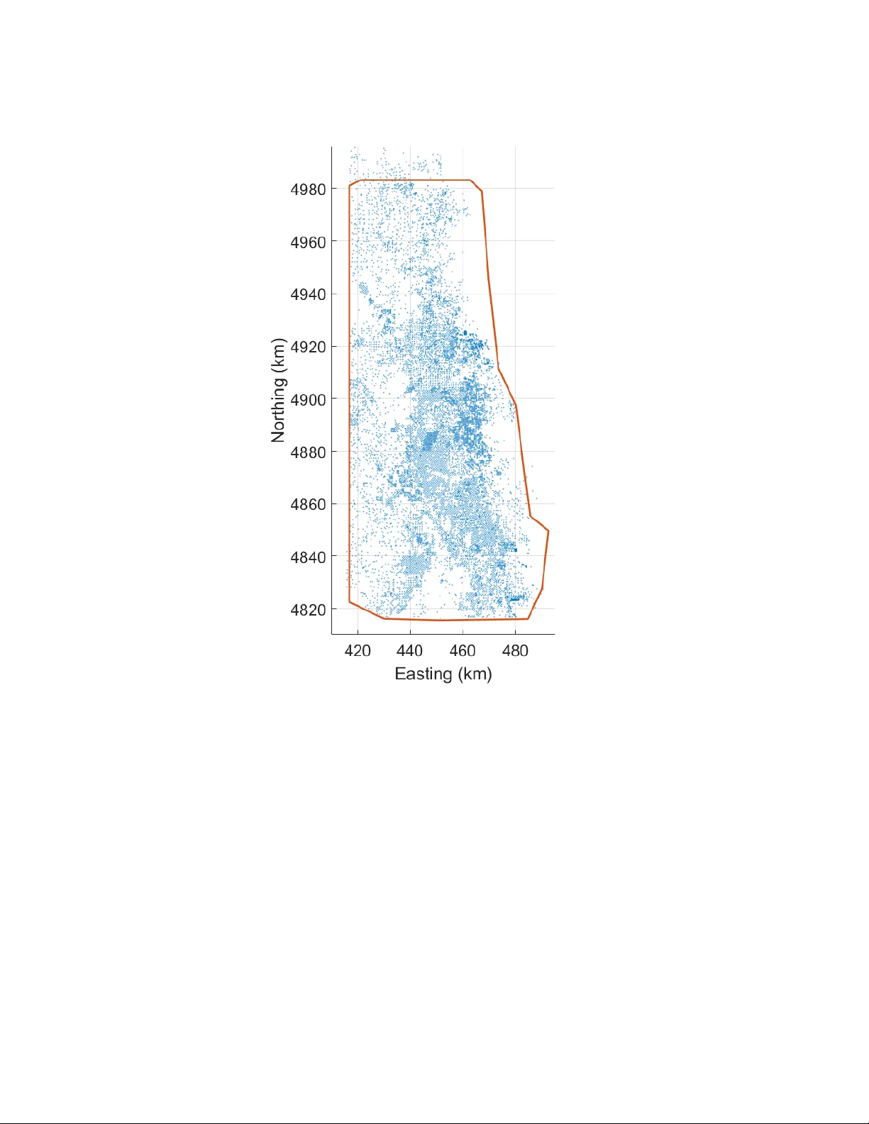
Sto c hastic Lo cal In teraction Mo del: Geostatistics without Kriging Dionissios T. Hristopulos, ∗ Andreas P avlides, V asiliki D. Agou, and P anagiota Gk afa Scho ol of Miner al R esour c es Engine ering, T e chnic al University of Cr ete, Chania 73100, Gr e e c e (Dated: Jan uary 9, 2020) Abstract Classical geostatistical metho ds face serious computational c hallenges if they are confronted with large sets of spatially distributed data. W e present a simplified stochastic local interaction (SLI) mo del for computationally efficien t spatial prediction that can handle large data. The SLI metho d constructs a spatial in teraction matrix (precision matrix) that accoun ts for the data v alues, their lo- cations, and the sampling densit y v ariations without user input. W e sho w that this precision matrix is strictly p ositiv e definite. The SLI approach does not require matrix inv ersion for parameter es- timation, spatial prediction, and uncertaint y estimation, leading to computational pro cedures that are significan tly less in tensive computationally than kriging. The precision matrix in volv es compact k ernel functions (spherical, quadratic, etc.) whic h enable the application of sparse matrix metho ds, th us impro ving computational time and memory requiremen ts. W e in vestigate the prop osed SLI metho d with a data set that includes approximately 11500 drill-hole data of coal thic kness from Campb ell Count y (Wy oming, USA). W e also compare SLI with ordinary kriging (OK) in terms of estimation p erformance, using cross v alidation analysis, and computational time. According to the v alidation measures used, SLI p erforms sligh tly b etter in estimating seam thickness than OK in terms of cross-v alidation measures. In terms of computation time, SLI prediction is 3 to 25 times (dep ending on the size of the kriging neigh b orhoo d) faster than OK for the same grid size. P A CS num b ers: 02.50.-r, 02.50.Tt, 02.60.Ed, 04.60.Nc, 05.50.+q, 89.30.A-, 89.60.-k ∗ dionisi@mred.tuc.gr 1 I. INTR ODUCTION Kriging and its v arious flav ors are the golden rule in geostatistics [3, 5, 6, 25, 31] and in mining applications of geostatistics in particular [2, 9, 19]. Ho wev er, the application of kriging to large datasets faces difficulties due to the computationally demanding in v ersion of the co v ariance matrix [29, 33]. Hence, v arious shortcuts and approximations hav e b een dev elop ed that allo w w orking with large datasets including the use of a finite searc h radius [26], tapered co v ariance functions [12], and fixed rank kriging [8]. F or reviews of the problem with large data see [20, 29]. F or data that are collected on rectangular grids there is an efficien t solution whic h is based on Gaussian Mark ov random fields (GMRFs) [27]. Ho wev er, this approach cannot b e directly extended to scattered data, although it is p ossible to generalize GMRFs b y linking them to sto c hastic partial differential equations [21]. The motiv ation for sto chastic lo c al inter action (SLI) mo dels is the p ossibilit y , known in the statistical field theories of physics and in Mark o v random field mo dels, to construct spatial and spatiotemporal dependence based on energy functions with lo c al inter actions . In statistical ph ysics this idea is presen t in the widely-used Boltzmann-Gibbs distributions that include the Gaussian field theory and the binary Ising mo del among others, e.g. [22]. Lo cal in teractions allow building sparse and explicit precision (inv erse cov ariance) ma- trices for the spatial dep endence. Hence, computationally fast algorithms can b e designed for sp atial pr e diction based on the conditional mean. The uncertain ty of the estimates is easily assessed by means of the c onditional varianc e whic h follows directly from the preci- sion matrix. The explicit form of the precision matrix implies indep endence from the curse of co v ariance matrix inv ersion, which plagues the application of geostatistical metho ds to large datasets. Hence, suc h mo dels can b e used as computationally efficien t alternatives to kriging. An SLI mo del that inv olves gradien t and curv ature terms w as presented in [17]. This mo del has a precision matrix that is not demonstrably non-negative definite, ev en though it is in practice w ell-defined in most cases. Herein w e presen t a simpler v ersion of the mo del whic h do es not include the curv ature term and p ossesses a positive definite precision matrix. The SLI mo del can b e view ed as an extension of Gaussian Markov r andom fields (GM- 2 RFs) [27] to scattered data b y means of kernel functions. F rom a differen t viewpoint, the SLI mo del can b e view ed as a discrete analogue of Spartan spatial random fields which are de- fined in contin uum space [13, 14, 16]. In order to accommodate random sampling geometries, the SLI mo del incorporates ideas from mac hine learning suc h as the use of k ernel functions. The range of the kernels is determined b y a set of lo cal bandwidths whic h is learned from the sample data. Hence, SLI prediction uses only a subset of the data for prediction at an y giv en p oin t. In kriging this restriction is imp osed by empirically determining a search neigh b orho od by trial and error. In the case of SLI, the range of the kernel is automatically adjusted b y the algorithm (see Section I I C). An additional adv antage of SLI o ver kriging is that the former do es not require co v ariance matrix inv ersion to compute the prediction and prediction uncertaint y . The remainder of this manuscript is structured as follows: Section I I presen ts the SLI metho dology , including the SLI model, the equations for prediction and conditional standard deviation, and the lea ve-one-out cross v alidation procedure for model parameter estimation. In Section II I the Campb ell coal dataset is briefly describ ed. Section IV presents the SLI mo del parameter estimation, while Section V fo cuses on the estimation of the v ariogram for ordinary kriging. Section VI provides the SLI-based and kriging-based estimates of coal resources and the asso ciated uncertainties. Section VI I studies the stability of the SLI estimates and compares the SLI and ordinary kriging predictiv e p erformance using lea ve-P- out cross v alidation. Finally , in Section VI I I we presen t our conclusions, discuss p oten tial applications of the metho d and analogies with other approaches, and outline directions for future research. I I. METHODOLOGY A. Notation In the follo wing, x S ≡ ( x 1 , . . . , x N ) > denotes the sample v alues at the lo cations of the sampling set S N = { s 1 , . . . , s N } , where s i ∈ D ⊂ R d , i = 1 , . . . , N . The sup erscript > denotes the matrix transp ose. The prediction set in volv es the p oin ts z p , p = 1 , . . . , P whic h 3 t ypically corresp ond to the no des of a map grid P ⊂ Z d . In general, S N and P are disjoin t sets. The SLI optimal prediction at these p oints will be denoted by ˆ x p . Assuming a constant mean, m x , fluctuations around the m ean will b e denoted b y primes, i.e., x 0 i = x i − m x . In case the mean is not homogeneous, a trend function is subtracted to obtain the fluctuations. The SLI mo del is defined is terms of the fluctuations. How ev er, the constan t mean or the trend function do not need to b e known a priori , since they can b e determined in the estimation stage. B. Kernel F unctions The SLI form ulation uses ideas from kernel r e gr ession [23, 32] in order to express the lo cal spatial dep endence. The interactions b et ween neighboring p oin ts are expressed in terms of suitably selected weigh ting functions, whic h are supplied by kernel functions. A k ernel (w eighting) function K ( s n , s m ) : R d × R d → R is a non-negative function that assigns a real v alue to any pair of p oin ts s n and s m . The range of the kernel is determined b y a c haracteristic length scale known as the b andwidth and denoted by h . The bandwidth should tend to zero as N → ∞ , so that for large and dense datasets emphasis is placed on p oin ts that are close to the target site. F or s n , s m ∈ R d let u = k s n − s m k /h represen t the normalized distance. A kernel function is (a) non-negative, i.e., K ( u ) ≥ 0 for all u ; (b) symmetric, i.e., K ( − u ) = K ( u ) for all u ∈ R 0 , + ; (c) maximized at u = 0; (d) a con tin uous function of u . A list of common k ernel functions is given in T able I. The first six functions of the table (triangular, Epanec hnik ov, quadratic, quartic, tricub e, spherical, Cauch y) are compactly supp orted, while the last tw o functions (exp onen tial, Gaussian) are infinitely extended but in tegrable. C. Kernel W eights The kernel functions can b e used to define w eights for the interaction b et w een t w o points s n and s m as follows 4 w ( r n,m ; h ) = K ( r n,m /h n ) P N k =1 P N l =1 K ( r k,l /h k ) , for n, m = 1 . . . , N , (1) where r n,m = s n − s m is the distance vector, while h n is a bandwidth sp ecific to the p oin t s n that reflects the sampling densit y around that p oin t. As a result of the lo cal bandwidth definition in (1), the k ernel w eights are not necessarily symmetric with respect to interc hange of the indices, i.e., in general w ( r n,m ; h ) 6 = w ( r m,n ; h ), since the local sampling densit y around the p oin t s n can b e quite different than the sampling densit y around s m . In general, one can consider N differen t bandwidths. Ho wev er, then the spatial mo del in volv es more parameters than data v alues, since the SLI mo del has other co efficien ts in addition to the bandwidths. It is b etter to define the lo c al b andwidths in terms of a small set of free parameters. An intuitiv e and flexible c hoice is to use h n = µ D n, [ k ] ( S N ) , (2) where h n is the bandwidth assigned to the p oin t s n , D n, [ k ] ( S N ) is the distance b etw een s n and its k -ne ar est neighb or in the sampling set S N , and µ > 0 is a p ositive bandwidth tuning parameter. The local distances D n, [ k ] ( S N ) can b e efficien tly computed using near-neighbor estimation algorithms, while the global co efficien t µ b ecomes a mo del parameter that is determined from the data via the cross-v alidation pro cedure as describ ed in Section I I G. The ab o v e definition of the bandwidth implies that larger bandwidth v alues are assigned to p oin ts in areas where the sampling is sparse. D. Gradien t-based SLI Energy F unction The SLI model is defined in terms of a Gibbs-Boltzmann exp onen tial join t densit y of the follo wing form [3] f ( x S ) = 1 Z ( θ ) e −H ( x S ; θ ) , 5 T ABLE I: List of common k ernel functions. The normalized distance u is giv en b y u = k r k /h . ϑ ( x ) = 1 if x ≥ 0 and ϑ ( x ) = 0 if x < 0 is the unit step function. Name Equation ( u ≥ 0) T riangular K ( u ) = (1 − u ) ϑ (1 − u ) Epanec hniko v K ( u ) = (1 − u ) 2 ϑ (1 − u ) Quadratic K ( u ) = (1 − u 2 ) ϑ (1 − u ) Quartic (biweigh t) K ( u ) = (1 − u 2 ) 2 ϑ (1 − u ) T ricub e K ( u ) = (1 − u 3 ) 3 ϑ (1 − u ) Spherical K ( u ) = (1 − 1 . 5 u + 0 . 5 u 3 ) ϑ (1 − u ) T runcated Cauc h y K ( u ) = 1 / (1 + u 2 ) ϑ (1 − u ) Exp onen tial K ( u ) = exp( − u ) Gaussian K ( u ) = exp( − u 2 ) where θ is the SLI parameter v ector that needs to b e determined from the data. The func- tion H ( x S ; θ ) is the energy of the SLI mo del whic h incorp orates the lo cal in teractions. The denominator Z ( θ ) is known in physics as the p artition function and represen ts a normaliza- tion constan t [22]. It will not b e necessary to ev aluate this constan t in order to estimate the parameters or to predict at non-measured p ositions. In the case of scattered data, a parsimonious SLI energy functional that includes squared fluctuation and squared “gradien t” terms is given b y [16] H ( x S ; θ ) = 1 2 λ  ( x S − m x ) > ( x S − m x ) N + c 1 S 1 ( x S ; h )  , (3) where m x is the v ector of the lo cal expected v alues (whic h is assumed constan t herein), λ is a sc ale c o efficient that is proportional to the o verall v ariabilit y of the data, c 1 > 0 is a p ositiv e rigidity c o efficient that weighs the cost of gradients in the data, S 1 ( x S ; h ) is the k ernel-av erage square gradien t, h = ( h 1 , . . . , h N ) > is a vector of lo c al kernel b andwidths that is used to determine the lo cal bandwidths, and θ = ( λ, m x , c 1 , k , µ ) > . The gr adient-b ase d ener gy terms are given b y the follo wing kernel a verage 6 S 1 ( x S ; h ) =  ( x n − x k ) 2  h = N X n =1 N X k =1 w ( r n,k ; h ) ( x n − x k ) 2 , (4) where  ( x n − x k ) 2  h represen ts the Nadaray a-W atson av erage [23, 32] of the square differ- ences of the data v alues. E. SLI Precision Matrix F orm ulation The SLI energy function (3) is a quadratic function of the sample v alues. Hence, it can b e equiv alently expressed in the following form that in v olves the precision matrix J ( θ ): H ( x S ; θ ) = 1 2 ( x S − m x ) > J ( θ ) ( x S − m x ) . (5) The precision matrix has the follo wing structure J ( θ 0 ) = 1 λ  I N N + c 1 J 1 ( h )  , (6a) and dep ends on the reduced parameter v ector θ 0 = ( λ, c 1 , k , µ ) > . In the ab o v e, I N is the N × N iden tity matrix which results from the energy of the squared fluctuations, and J 1 ( h ) is the gr adient pr e cision sub-matrix which results from the sum of the squared differences and is given b y [ J 1 ( h )] n,m = − w n,m ( h ) − w m,n ( h ) + δ n,m N X k =1 [ w n,k ( h ) + w k,n ( h )] , (6b) where w n,m ( h ) = w ( r n,m ; h ) is an abbreviation of the kernel w eights (1) and δ n,m = 1 if m = n while δ n,m = 0 if m 6 = n is the Kr one cker delta . Theorem 1. The SLI pr e cision matrix define d by (6) is strictly p ositive definite for λ > 0 and c 1 > 0 . Mor e over, it is diagonal ly dominant. Pr o of. The matrix J ( θ 0 ) is p ositiv e definite if it is real-v alued and symmetric, ev ery non-zero x = ( x 1 , . . . , x n ) > and every n ∈ N it holds that x > J ( θ 0 ) x ≥ 0 . The matrix J ( θ 0 ) defined b y (6) is real-v alued and symmetric b y construction. In addition, if w e set x 0 = x S − m x , it 7 follo ws from (5) that x 0 > J ( θ 0 ) x 0 = 2 H ( x ). This equation holds for an y sample x S and for an y m x ∈ R , thus for all p ossible x . Ho wev er, the energy is equiv alently expressed based on (3) as follo ws 2 H ( x ; θ ) = 1 λ " x 0 > x 0 N + c 1  ( x n − x k ) 2  h # . It is straigh tforward to sho w based on (3) and (4) that since c 1 , λ > 0, the energy is strictly p ositiv e for any non-zero vector x 0 . If all the en tries of the v ector x 0 tak e the same v alue, the gradien t term, whic h is prop ortional to c 1 , v anishes; ho wev er, the first term is still p ositiv e. Hence, the matrix J ( θ 0 ) is strictly p ositive definite . Diagonal dominance requires that for all n = 1 , . . . , N the following condition b e satisfied | J n,n | ≥ N X m 6 = n =1 | J n,m | . The diagonal dominance condition is stricter than positive definiteness. Hence, the former implies the latter (but not vice v ersa). F rom (6) it follows that J n,n = 1 N λ + c 1 λ N X m 6 = n =1 ( w n,m + w m,n ) , (7a) J n,m = − c 1 λ ( w n,m + w m,n ) , m 6 = n. (7b) Based on the ab o ve and the non-negativity of the weigh ts, i.e., w n,m ≥ 0 for all m, n = 1 , . . . , N , it follo ws that | J n,n | − N X m 6 = n =1 | J n,m | = 1 / N λ. Hence the diagonal dominance of the SLI precision matrix is prov ed. 8 F. SLI Prediction In this section we sho w ho w to use the SLI mo del to estimate the unknown v alues of the field at the sites z p ∈ P . Let us consider that one the prediction p oin ts z p is added to the sampling netw ork. The SLI energy function is then mo dified as follows: ˆ H ( x S , x p ; θ ) = H ( x S ; θ ) + J p,p x 0 2 p 2 + 1 2 N X n =1 ( J n,p + J p,n ) x 0 p x 0 n . (8) The first term in (8) is the sample energy (3), while the second and third terms represent the additional energy con tribution that in v olves z p : the second term is the self-interaction of the prediction p oin t which con tributes prop ortionally to the square of the fluctuation, and the third term inv olv es the interaction of the prediction p oin t with the sampling p oints. The latter represents lo cal gradien ts that reflect differences b etw een the fluctuation at z p and neigh b oring sample p oints. The energy (8) determines the conditional probabilit y densit y function at the prediction p oin t, which is giv en b y f ( x p | x S , θ ) ∝ exp h − ˆ H ( x S , x p ; θ ) i . (9) The optimal SLI prediction at z p is equal to the v alue that minimizes the energy (8) and th us maximizes the conditional p df. This v alue is a stationary p oin t of the energy , i.e., it satisfies ˆ x p = arg min x p ˆ H ( x S , x p ; θ ∗ − λ ) , where θ ∗ − λ denotes the optimal p ar ameter ve ctor (excluding λ ) whic h is estimated from the data as shown in Section I I G. F or now w e assume that θ ∗ − λ is known. The first term in (8) excludes the prediction p oint and th us it drops out in the minimiza- tion. The first-order deriv ativ es of the next t w o energy terms lead to a linear equation for the stationary p oint, whic h admits the follo wing unique solution 9 ˆ x p = m x − 1 J p,p ( θ ∗ ) N X n =1 J p,n ( θ ∗ ) ( x n − m x ) . (10) In (10) we used the symmetry of the precision matrix, i.e., the fact that J p,n = J n,p . The precision matrix entries that inv olve the prediction p oin ts are obtained from (7) as follo ws J p,p ( θ ∗ ) = 1 N λ ∗ + c ∗ 1 λ ∗ N X n =1 ( w n,p + w p,n ) , (11a) J p,n ( θ ∗ ) = − c ∗ 1 λ ∗ ( w n,p + w p,n ) . (11b) In ligh t of the k ernel weigh t definition (1), the summands in (11a) are either zero (if the distance b et ween s n and z p exceeds the lo cal bandwidth) or p ositiv e (otherwise). The predictor (10) is a stationary p oin t of the energy . It remains to v erify that it represen ts the minim um so that the prediction corresp onds to the mo de of the conditional p df (9). The second-order deriv ativ e of the energy (8) with resp ect to x p is given by J p,p . According to (11) it holds that J p,p > 0 since λ ∗ , c ∗ 1 > 0 and the k ernel weigh ts are p ositiv e. Hence the predictor indeed corresp onds to the global minim um of the energy . a. Pr op erties of the SLI pr e dictor 1. Note that the prediction equation (10) is analogous to the equation that determines the conditional mean in GMRFs. This is not surprising since the SLI predictor finds the minimum energy at the prediction p oin t, conditionally on the sample v alues. 2. The SLI predictor is unbiase d as can b e seen from (10): the second term on the righ t hand side, which is prop ortional to the fluctuations, v anishes up on calculating the ensem ble av erage. 3. The SLI predictor is not an exact in terp olator. According to (10), exactitude requires that if z p → s n ∗ ∈ S N then J p,n = 0, for all n 6 = n ∗ . This could only o ccur if the bandwidth tends to zero, or if it is sufficien tly small to exclude all other p oin ts b esides s n ∗ for all n ∗ ∈ { 1 , . . . , N } . How ever, the difference b et ween the SLI prediction and 10 the true v alue is usually negligible. This is due to the fact that the sample v alue at the nearest point to the prediction lo cation has the largest linear SLI w eight and hence the most impact on the prediction. 4. The prediction is indep enden t of the sc ale c o efficient λ . This b ecomes ob vious up on insp ection of (10), since the prediction inv olves the ratio of precision matrix elemen ts. 5. The analogy of SLI with GMRFs allo ws us to calculate the c onditional varianc e at the prediction p oin t as σ 2 p = 1 J p,p ∝ λ ∗ . (12) The conditional v ariance endo ws the SLI metho d with a measure of pr e diction unc er- tainty which is analogous to the kriging v ariance. Just lik e the kriging v ariance, the SLI conditional v ariance do es not explicitly dep end on the data v alues. It only dep ends indirectly to the exten t that the data influence the mo del parameters. b. Computational efficiency: The n umerical cost of the prediction equation (10) is pro- p ortional to N . Since the predictor is applied P times to generate the map grid, the n u- merical complexity is O ( N P ). According to (11) the numerical complexity of calculating the precision matrix is O ( N ) p er prediction p oin t; therefore the o verall complexit y is again O ( N P ). How ever, the kernel w eigh ts (1) inv olve a double summation o ver the sampling p oin ts which has a computation complexity O ( N β ), where 1 < β ≤ 2. The maximum complexit y rate, β = 2, is obtained for infinite-support k ernels. F or compactly supp orted k ernels, rates β < 2 can b e ac hiev ed. In general, the upp er b ound of the SLI computational complexit y is O ( N 2 + N P ). The memory space required for storage of the precision matrix scales as O ( q N 2 ), where q is the sp arsity of the precision matrix; for compactly supported k ernels typically q  1. Kriging has a numerical complexit y O ( N 3 ) for the inv ersion of the cov ariance matrix, and O ( N 2 + N P ) for the calculation of the kriging weigh ts and the prediction [33]. The kriging complexit y is practically dominated b y the inv ersion of the cov ariance matrix. In addition, kriging requires the storage of the cov ariance matrix whic h consumes O ( N 2 ) of memory space. The computational requirements of kriging can b e reduced by introducing 11 v arious mo difications, e.g., using searc h neigh b orho o ds with a small n umber of sampling p oin ts around eac h prediction point [25] or b y means of tapered co v ariance functions that ha ve compact supp orts [12]. G. SLI P arameter Estimation The SLI parameter v ector is giv en b y θ = ( λ, m x , c 1 , k , µ ) > . In addition to the data, the estimated θ also depends on the kernel function. W e use the follo wing approac h to estimate the SLI mo del parameters from the data: 1. The mean m x is set equal to the sample a verage. This is a reasonable c hoice in the absence of spatial trends, esp ecially for large datasets. Ho wev er, it is also p ossible to consider m x as a parameter to b e determined from the data by means of cross v alidation as sho wn by Hristopulos and Agou [18]. 2. The order k of the near-neigh b or used to estimate the lo cal bandwidths according to (2) is t ypically assigned an in teger v alue determined by exp erimentation with the data. Herein we use k = 3; we justify this c hoice b elo w. 3. The optimal rigidit y coefficient c ∗ 1 and global bandwidth parameter µ ∗ are determined b y means of lea ve-one-out (LOO) cross-v alidation (CV). In LOO CV sample p oin ts are remov ed one at a time. Their v alues are then estimated b y means of the remaining N − 1 sample p oin ts and the SLI prediction equation (10). After all the p oin ts are remo ved and estimated, a sp ecified validation me asur e (e.g., mean absolute error, root mean square error) that quantifies the discrepancy b et ween the estimates and the true v alues is calculated. The v alidation measure is used as the c ost function for the optimization of the SLI parameters. 4. The optimal v alue of the scale co efficien t is determined by means of [17] λ ∗ = 2 H ( x S ; θ ∗ − λ ) N , where θ ∗ − λ = (1 , m ∗ x , c ∗ 1 , k ∗ , µ ∗ ) > . (13) 12 The v alue of λ ∗ is only used in determining the conditional v ariance but not for pre- diction. The abov e pro cedure is rep eated for differen t c hoices of the kernel function, and the kernel mo del whic h optimizes the cost function is selected. Maxim um lik eliho o d estimation (MLE) is also p ossible within the SLI framew ork. Ho w- ev er, in using MLE we are forced to estimate the partition function, Z ( θ ), which in v olves calculating the determinant of the large, alb eit sparse, precision matrix J ( θ 0 ). I I I. DESCRIPTION OF THE D A T A AND STUD Y AREA W e apply the SLI mo del to a set of coal thickness data from 11416 drill-holes. The data come from the Gillette field in Campb ell Coun ty , Wyoming (USA). The lo cations of the drill-holes are sho wn in Fig. 1. Campb ell Coun ty lies within the P owder Riv er Basin and includes tw o of the largest coal mines in the world: North Antelope Ro c helle coal mine and Blac k Th under coal mine. The Gillette coal field con tains significan t quan tities of exploitable coal resources that are low in sulfur and ash con tent. The study domain extends o ver an area that cov ers appro ximately 9500 km 2 . W e fo cus on coal beds from the upp er part of F ort Union F ormation whic h include the Roland b ed and coal in the Wyodak-Anderson zone. The stratigraphic cross-section show casing the Wy o dak-Anderson coal zone for part of the Gillette Field is sho wn in Fig. 2. The geological formations present in the Gillette field are sho wn in Fig. 3 [11]. Coal from the Wyodak zone has higher mean gross calorific v alue (4760 k cal/kg), lo wer mean ash yield (5.8%), and low er mean total sulfur conten t (0.46%) compared with the resp ectiv e v alues for the com bined Wy o dak-Anderson coal zones [10]. The main statistics of the marginal distribution of the coal thickness data are listed in T able I I. The frequency histogram which represents the empirical probabilit y distribution of the thickness v alues is shown in Fig. 4. Both the statistics shown in T able I I and the histogram in Fig. 4 sho w evidence of mild deviation from the normal (Gaussian) distribution. The spatial distribution of the drill-holes, and hence the sampling densit y , v aries significan tly 13 FIG. 1: Drill-hole lo cations of the coal thic kness data from the Gillette field. The red line represen ts the b order of the area within which the resources will b e estimated. in space as evidenced in Fig. 1. The median of the nearest distance b etw een drill-holes is 458 m. All the n umerical tests b elo w are conducted and timed on a desktop computer running Windo ws 10 operating system equipped with In tel(R) Core(TM) i7-6700K CPU @ 4.00GHz and 16.0 GB RAM installed. The n umerical implemen tation w as p erformed in the MA TLAB programming environmen t (release R2016a). 14 FIG. 2: Structural cross section showing the Wyodak-Anderson coal zone (W-A Zone) of the Gillette coalfield [28]. T ABLE I I: Statistics of coal thic kness in the upp er part of F ort Union F ormation based on data from the 11416 drill-hole lo cations of Gillette Field. Mean (m) Median (m) Maxim um (m) Minimum (m) Standard deviation (m) Sk ewness 7.83 7.71 22.67 0.33 2.99 0.13 IV. SLI MODEL ESTIMA TION F OR GILLETTE FIELD T o use SLI for interpolation we first need to estimate the mo del parameters from the Gillette field coal data. W e p erform this task using LOO-CV as describ ed in Section I I G. Kernel weigh ting functions are utilized in the SLI predictions as explained in Section I I B to determine the weigh ts given b y equation (1). T o find the optimal k ernel function we use LOO-CV on the en tire dataset and select the kernel function that optimizes the CV cost function. Herein we use the mean absolute error (MAE) as the cost function. The optimization is p erformed in the Matlab environmen t using the constrained minimization function fmincon with the interior-point algorithm [24]. 15 FIG. 3: Section sho wcasing geological formations and coal zones for the Gilette Field [28]. A. Kernel function selection W e compare the predictiv e p erformance of different compactly supp orted k ernels from the list shown in T able I. Compact kernels lead to sparse precision matrices (see Section I I E) that are computationally less in tensiv e for big datasets. The comparison is based on the mean absolute error obtained by means of lea ve-one-out cross v alidation. The SLI predictions are based on the equation (10). T able I I I sho ws the cross-v alidation MAE for the differen t k ernel functions obtained using neigh b or order k = 3 to define the distances D n, [ k ] ( S N ) in equation (2). As is evidenced T able I II, the parameter c 1 that con trols the gradien t precision sub-matrix (6a) tak es v alues close to 115 for all the k ernels. The bandwidth con trol parameter µ shows more dependence 16 FIG. 4: F requency histogram of the coal thickness distribution in the upp er part of F ort Union F ormation based on data from 11416 drill holes in Gilette field. on the k ernel function. The MAE takes very similar v alues for all the studied k ernels, ranging b et w een 1 . 12 m and 1 . 13 m (truncating at tw o decimal p oints). Based on these results w e select the spherical k ernel whic h giv es one of the lo w est MAE (slightly less than 1 . 12 m). The Epanechnik o v k ernel also returns practically the same MAE v alue, but a higher v alue for µ ; as the latter determines the bandwidth, higher v alues of µ imply increased memory requiremen ts and computational time. In general, w e exp ect that an y of the kernels listed in T able II I (except for the uniform kernel which has a slightly higher MAE) will lead to comparable p erformance. B. Distribution of SLI bandwidths The distribution of bandwidths for the spherical k ernel is sho wn in the histogram plot of Fig. 5. The bandwidths are obtained from (2) using k = 3 and µ = 2 . 3675. As evidenced in the histogram plot, the bandwidth distribution is disp ersed with a p eak at ≈ 1500 m; ho wev er, there are also v alues as large as 8000 m. The dispersion of the distribution reflects the v ariations of the sampling density (cf. Fig. 1) in Gillette field: Larger (smaller) v alues 17 T ABLE I II: Comparison of the mean absolute error (MAE) v alue in coal thickness estimation by SLI using different k ernel functions with neighbor order k = 3 and initial parameter v alues c (0) 1 = 115 and µ (0) = 1 . 5. MAE is optimized by means of a constrained optimization metho d. The v alue of µ is constrained in the interv al [0 . 5 , 5], and c 1 ∈ [eps , ∞ ], where eps ≈ 2 . 22 × 10 − 16 is the floating-p oint relativ e accuracy . Kernel c 1 µ λ MAE (m) Uniform 115 . 0000 1 . 5000 0 . 1949 1 . 1315 T riangular 115 . 0003 2 . 0018 0 . 1802 1 . 1213 Quadratic 115 . 0003 1 . 8958 0 . 1907 1 . 1228 Biw eight 115 . 0002 2 . 1772 0 . 1859 1 . 1209 T ricubic 115 . 0002 2 . 1885 0 . 1891 1 . 1215 Epanec hniko v 115 . 0003 2 . 4526 0 . 1676 1 . 1199 Spherical 115 . 0003 2 . 3675 0 . 1727 1 . 1199 T ABLE IV: Comparison of the mean absolute error (MAE) v alue in coal thic kness estimation by SLI using the spherical k ernel function with neighbor order k = 2 , 3 , 4 and initial parameter v alues c (0) 1 = 115 and µ (0) = 1 . 5. The v alue of µ is constrained in the in terv al [0 . 5 , 5], and c 1 ∈ [eps , ∞ ]. The computational time was b et ween 5 and 9 min utes. Neigh b or order c 1 µ λ MAE (m) k = 2 115.0003 2.6795 0.1671 1 . 1182 k = 3 115.0003 2.3675 0.1727 1.1199 k = 4 115.0002 2.0518 0.1717 1.1188 of the bandwidth are obtained in areas of sparser (denser) sampling. The c hoice of neighbor order k = 3 is based on T able IV, whic h compares the parameter estimates and the MAE v alues obtained for three differen t neigh b or orders: k = 2 , 3 , 4. The table shows that k = 2 giv es the low est MAE; how ever, all the MAE are equal within the second decimal place. In order to be impartial in our selection w e c ho ose k = 3. As the neigh b or order k increases, the optimal µ decreases (see T able IV), th us tending to k eep the v alue of the optimal bandwidth constan t. This b eha vior further demonstrates the ability of SLI to adjust the bandwidth adaptiv ely without user input. 18 FIG. 5: F requency histogram of the kernel bandwidths (m) used in the SLI metho d. The bandwidths were determined from (2) using the spherical k ernel with near-neigh b or order k = 3. C. P arameter estimation using global optimization Note that the estimated c ∗ 1 = 115 . 0003 is very close to the initial guess c (0) 1 = 115. This result suggests that the optimization, whic h is p erformed by means of the constrained optimization Matlab function fmincon with an in terior-p oin t algorithm, ma y b e stuck in a lo cal minim um. T o inv estigate this p ossibilit y w e use the global searc h optimization function in Matlab, which can find global solutions to problems that contain multiple maxima or minima. This pro cedure is time intensiv e, but it allows for a b etter exploration of the SLI parameter space. W e use the Matlab GlobalSearch solv er whic h generates a sequence of starting p oin ts (initial guesses) in com bination with the interior-point lo cal optimization 19 routine [30]. The global optimizer is run with differen t initial v alues and b ounds for c 1 . The results of global optimization for four different combinations of initial v alues and b ounds for c 1 are rep orted in T able V. All runs take sev eral hours to complete, due to the exhaustiv e search of the parameter space b y the global optimizer. As evidenced in T able V the global optimizer giv es differen t solutions dep ending on the initial conditions. These solutions are in a different region of parameter space than the lo cal optim um ( c ∗ 1 ≈ 115 , µ ∗ ≈ 2 . 37 , λ ∗ ≈ 0 . 17). Ho wev er, all the solutions lead to v ery similar results for the cost function (i.e., the MAE). This in vestigation sho ws that differen t lo cal minima of the SLI cost function are essentially identical with resp ect to prediction performance. W e further discuss this issue in Section VI I. Note that b oth the global and lo cal solutions giv e essen tially the same estimate for µ ∗ . At the same time, the ratio c ∗ 1 /λ ∗ is also approximately the same for b oth the global ( ≈ 670) and the lo cal ( ≈ 676) estimates. This observ ation is further analyzed and justified in Section VI I A. T ABLE V: Estimates of SLI parameters using LOO-CV and optimal mean absolute error (MAE) for the coal thickness data. The estimates are deriv ed using the Matlab global optimization solver GlobalSearc h with differen t initial guesses and constraint in terv als for c 1 . The SLI mo del is implemented using the spherical k ernel function with neighbor order k = 3. The parameter µ is constrained in the in terv al [0 . 5 , 5] and its initial guess is µ (0) = 1 . 5. Constrain ts and Initialization c ∗ 1 µ ∗ λ ∗ MAE (m) c ∗ 1 /λ ∗ c 1 ∈ [eps, ∞ ], c (0) 1 = 115 1 . 0001 × 10 4 2 . 3742 14 . 9147 1 . 1996 670.48 c 1 ∈ [10 , 10 8 ], c (0) 1 = 115 7.3092 × 10 7 2.3743 1.0900 × 10 5 1 . 1196 669.72 c 1 ∈ [eps, ∞ ], c (0) 1 = 10 8.3285 × 10 13 2.3762 1.2427 × 10 11 1.1196 669.91 c 1 ∈ [10 , 10 8 ], c (0) 1 = 10 8.2394 × 10 7 2.3743 1.2287 × 10 5 1.1196 670.58 V. V ARIOGRAM MODELING In this section we estimate the v ariogram model that will b e used for ordinary kriging in terp olation and resources estimation. W e use the robust v ariogram estimator [7] for the empirical v ariogram of coal thickness whic h w e then fit to five common v ariogram mo dels. The robust v ariogram estimator is giv en b y 20 ˆ γ ( r ) =  1 2 N ( r ) P N ( r ) i =1 | x ( s i ) − x ( s i + r ) | 1 / 2  4 0 . 457 + 0 . 494 N ( r ) + 0 . 045 N 2 ( r ) , (14) where r is the distance (lag) vector b et w een t wo p oin ts and N ( r ) is the num b er of pairs separated by r . W e used (14) to calculate the omnidirectional v ariogram. W e then tested fiv e different the- oretical v ariogram mo dels (Spherical, Cubic, Gaussian, P o wer, and Exp onen tial) com bined with a n ugget term. The fits of the theoretical models γ ( r ; θ ) to the empirical v ariogram are presen ted in Fig. 6. The b est fitting model was selected b y minimizing the sum of weigh ted squared errors giv en by (15). The sum of weigh ted squared errors for the fiv e v ariogram mo dels tested are sho wn in T able VI. The spherical mo del is sho wn to minimize the sum of weigh ted squared errors. The optimal parameters for the spherical v ariogram mo del are sho wn in T able VI I. ε ( θ ) = L X i =1 [ γ ( r i ; θ ) − ˆ γ ( r i )] 2 γ 2 ( r i ; θ ) (15) T ABLE VI: Sum of w eighted squared errors b et ween the empirical v ariogram and the five theoretical mo dels that are tested based on equation (15) (units are in m 4 ). V ariogram Mo del Gaussian Cubic Spherical Po w er Exponential Fitting Error ε ( θ ) 11.55 2.67 1.92 6.79 3.37 T ABLE VI I: P arameters of the optimal spherical v ariogram mo del: σ 2 is the correlated v ariance, ξ is the correlation length, and c 0 is the nugget v ariance. The parameters are estimated by minimizing the error function (15). σ 2 (m 2 ) ξ (km) c 0 (m 2 ) 8.05 29.1 1.07 The optimality of the spherical function for b oth the v ariogram model and the SLI spher- ical kernel is coincidental. The spherical v ariogram mo del implies a spherical cov ariance, 21 FIG. 6: Robust v ariogram estimator (circles) and optimal fits to theoretical mo dels (Gaussian, Spherical, Po w er, Exp onen tial, and Cubic). The horizon tal axis is the lag distance k r k . The v ertical axis represen ts the v ariogram v alues of coal thic kness. while the spherical kernel in SLI en ters in the precision matrix. Finally , w e used the om- nidirectional v ariogram estimator and did not consider anisotropic v ariogram models. W e estimated geometric anisotrop y using the metho d of co v ariance Hessian identit y [4, 15]. This led to an estimate of the correlation length ratio along the tw o principal directions sligh tly less than tw o, which is considered as marginally isotropic. 22 VI. ESTIMA TION OF COAL RESOUR CES In this section w e estimate the coal resources of Gillette field using SLI and ordinary kriging. Our goal is to compare the SLI predictions with those of ordinary kriging. This comparison allo ws assessing the in terp olation p erformance of SLI against an established sto c hastic metho d. The estimate of the resources is based on estimated coal thickness v alues at the no des of an interpolation grid. The interpolation domain (contained inside the red- line b order in Fig. 1) is co v ered b y a map grid comprising 661355 orthogonal (appro ximately square) cells. The cell size is 114.7 m × 134.7 m. A. SLI Estimation of Coal Resources The coal dep osits in the upp er part of F ort Union F ormation in Gillette field are estimated b y SLI in terp olation at a total volume equal to V = A c P X p =1 ˆ x ( z p ) = 74 . 1 × 10 9 m 3 , (16) where A c is the surface area of the in terp olation grid cell and { ˆ x ( z p ) } P p =1 the estimated coal thic kness for the lay ers describ ed in Section I II at the cen ter p oin ts of the grid. These estimates are based on the spherical k ernel function and the mo del parameters of T able II I. The SLI metho d estimates b oth the most probable coal thic kness at each p oin t and the resp ectiv e prediction v ariance. The coal thickness prediction map is sho wn in Fig. 7a. The standard deviation of the SLI prediction, i.e., the square ro ot of the conditional v ariance of the SLI predictor giv en b y (12), is shown in Fig. 8a. An interesting feature of the SLI standard deviation map is the low uncertain ty v alues near the Northeastern b order of the study area which is a region of low sampling densit y . Ho wev er, as w e show in Fig. 8, b oth the bandwidth and the num b er of SLI neigh b ors (i.e., sampling p oints that are coupled with the prediction point via the SLI mo del) are rather high (i.e., more than 600) near the b oundary . Hence, the uncertaint y in this area is constrained b y a large, alb eit distan t, n umber of neighbors. The bandwidth for eac h prediction p oin t is 23 (a) SLI Map (b) SLI StD FIG. 7: SLI estimates of coal thic kness and standard deviation σ SLI for the upp er part of F ort Union F ormation in Gillette field. determined via the optimization pro cess based on the neigh b or order, the k ernel function, and the parameter µ . The bandwidth v alues can th us v ary considerably . This is in con trast with fixed-radius kriging, which maintains a constant search radius for all the prediction p oin ts. The n umber of SLI neigh b ors for each prediction p oin t is determined by the local bandwidth and the sampling p oin t configuration. An insp ection of the SLI standard deviation map (Fig. 8a) and the map of lo cal neigh b ors (Fig. 8b) sho ws that the n um b er of neigh b ors is correlated with the SLI standard deviation. The SLI uncertaint y seems to b eha ve more lik e 24 the standard deviation deriv ed from several sto c hastic sim ulations, in which the uncertain ty is proportional b oth to the data spacing and to the complexity in the fluctuations, than like the kriging standard deviation. (a) Log bandwidth (b) Local neigh b ors FIG. 8: (Left): Logarithm of the SLI bandwidth o ver the map area. (Right): Logarithm of n umber of neigh b ors p er map grid p oin t. B. OK Estimation of Coal Resources F or the estimation of the coal resources in the study area and the visualization of the spatial distribution of coal thickness w e use an OK interpolation grid iden tical with the SLI grid. W e tested four different circular searc h neigh b orhoo ds. The resp ectiv e searc h radii are equal to 1.5 km, 5.7 km, 9.1 km and 14.6 km. These v alues were guided by the correlation 25 length of the selected spherical mo del ( ≈ 29 km). W e implemen ted LOO-CV for each searc h radius, using the same v ariogram parameters (shown in T able VI I). Results for cross v alidation measures obtained with the searc h radii of 9.1 km and 14.6 km are sho wn in T able VI I I. There is no significan t difference b et ween the CV measures obtained with these radii and those obtained with radii of 1.5 km and 5.7 km. F or the purp ose of mapping the coal thic kness w e use the radius of 14.6 km b ecause it allows almost full co verage of the map grid. The resulting kriging maps of coal thic kness and it s standard deviation are sho wn in Figure 9. Note that the colorbar scale next to the OK standard deviation extends to v alues less than 1 m, i.e., low er than the n ugget standard deviation ( ≈ 1 m). This is due to using common color scales for the OK and SLI maps. The v alues of the OK standard deviation are actually larger than the n ugget standard deviation. Based on ordinary kriging the coal dep osits are estimated at 72.4 × 10 9 m 3 , using the spherical v ariogram mo del and mo del parameters of T able VI I with neigh b orho od 14.6 km. The SLI prediction takes ≈ 12 min, while kriging with a searc h radius of 9.1 km (14.6 km) tak es ≈ 42.7 min ( ≈ 319.2 min). C. Metho d Comparisons In this section we compare the p erformance of SLI and OK interpolation in terms of (i) the LOO-CV error of the coal thickness estimates (ii) v arious cross v alidation statistics and (iii) the interpolated maps of coal thic kness. First, we focus on the lea v e-one-out cross v alidation error whic h is given b y  ( s i ) = x ( s − i ) − ˆ x i ( s i ; θ ∗ i ) , i = 1 , . . . , N , where ˆ x − i ( s i ; θ ∗ i ) is the SLI (OK) estimate at the point s i based on the remaining N − 1 p oin ts and the parameter vector estimate deriv ed from the N − 1 p oin ts. The histograms of the LOO-CV errors are sho wn in Fig. 10 and exhibit ov erall go o d agreemen t. The error distributions are symmetric, reflecting the unbiasedness of the SLI and OK predictors. The v ast ma jorit y of the error v alues are distributed b et w een − 5 m and 26 FIG. 9: (a) Map of coal thic kness based on ordinary kriging. (b) Map of OK standard deviation σ OK . Both maps are obtained using the spherical v ariogram mo del with the optimal parameters (see T able VI I) and a search neigh b orho od of 14.6 km. 5 m. How ev er, there are a few error v alues with magnitudes b et w een 5m and 10 m as w ell as some v alues with larger magnitude. Figure 10 also exhibits b o x plots of the LOO-CV errors. The cen tral mark of the b ox plots is the median of the empirical distribution, and the edges of the b o x corresp ond to the 25th and 75th p ercen tiles. The whiskers extend to the most extreme v alues that are not considered outliers. V alues are considered as outliers if they lie outside the range [ q 3 − 1 . 5( q 3 − q 1 ) , q 3 + 1 . 5 ( q 3 − q 1 ) ], where q 1 and q 3 are the 25th and 75th percentiles of the sample data. This range corresp onds to the 99.3% probability interv al for the normal distribution. 27 Outliers are plotted as individual p oints (mark ed by crosses). A comparison of the tw o b o x plots sho ws that the SLI error is less disp erse, while the OK error has more w eight in the tails of the distribution, including a couple of v alues with magnitudes ab o v e 15. FIG. 10: Left: Histograms of the SLI (blue online) and OK (y ellow online) lea ve-one-out cross v alidation errors. The SLI parameters are given in T able I II. The spherical v ariogram parameters used in OK are giv en in T able VI I.A kriging searc h radius of 9.1 km is used. Righ t: Bo x plots of the SLI and OK errors (see text for definition of the b o x plot elements). Next, w e compare the predictiv e p erformance of SLI and OK in T able VI I I by means of cross-v alidation statistics. The following cross-v alidation measures are considered: 1. Mean Error (ME) to represent bias. 2. Mean Absolute Error (MAE). 3. Ro ot Mean Square Error (RMSE). 28 4. P earson’s linear correlation co efficien t ( R ). 5. Maxim um Absolute Error (MaxAE). 6. Mean Absolute Relativ e Error (MARE). 7. Ro ot Mean Square Relativ e Error (RMSRE). The SLI estimates ha ve lo w er mean absolute error, ro ot mean square error, maxim um absolute error and higher correlation co efficien t than the kriging estimates. On the other hand, kriging shows less bias, and lo wer relativ e MAE and RMSE. T ABLE VI II: LOO-CV measures of coal thickness based on (i) ordinary kriging with the spherical v ariogram mo del and (ii) SLI with spherical k ernel and neigh b or order k = 3. The v ariogram parameters are given in T able VI I and the SLI parameters are giv en in T able I II. A kriging search radius equal to 9.1 km is used. The following v alidation measures are shown: MAE: mean absolute error; MaxAE: Maxim um absolute error; MARE: mean absolute relativ e error; RMSE: ro ot mean square error; RMSRE: ro ot mean square relative error; R : Pearson’s correlation co efficien t. S.R.: Searc h radius. Metho d ME (m) MAE (m) MARE RMSE (m) RMSRE MaxAE (m) R (%) OK (9.1 km S.R.) 4.0224 × 10 − 4 1.1788 0.2480 1.8067 0.8312 16.7286 80.27% OK (14.6 km S.R.) 4.0573 × 10 − 4 1.1787 0.2480 1.8066 0.8313 16.7290 80.27% SLI ( k = 3) 5.6420 × 10 − 4 1.1199 0.2480 1.7033 0.8527 14.8781 82.23% Finally , the difference b et ween the SLI and OK estimates of coal thic kness ov er the map grid is illustrated in Fig. 11. The four interv als used are defined as follo ws: OK > SLI cor- resp onds to differences less than − 1m (higher OK estimates), OK=SLI includes differences b et w een − 1m and 1m, SLI > OK contains differences b etw een 1 and 3.5m, and SLI  OK differences higher than 3.5m. The difference b et w een the SLI and OK predictions ranges from − 7 . 6 m (higher OK estimates) to 9.67 m (higher SLI estimates). Figure 11a shows that the SLI estimate of coal thic kness at most map grid lo cations is appro ximately equal to OK estimates. A t lo cations where this is not true, SLI estimates tend to exceed the OK estimates more frequen tly than the opp osite. This leads to the ov erall higher SLI-based estimate of resources (74 . 1 × 10 9 m 3 v ersus 72 . 4 × 10 9 m 3 based on OK). 29 Regarding the spatial distribution of prediction uncertaint y , Fig. 11b sho ws that the SLI standard deviation in most places exceeds the OK standard deviation. This is not surprising, since the OK predictor is constructed based on the minimization of the mean error v ariance while the SLI metho d do es not constrain the v ariance. A t the same time, there are spatial p ock ets where the SLI uncertaint y is low er than the resp ectiv e OK v alue. A juxtap osition of the plots in Fig. 11b and Fig. 8 shows that areas with lo w er SLI v ariance (e.g., near the northeastern b order of the study domain) coincide with areas that hav e high bandwidth and, esp ecially , high num b er of SLI neighbors. The presence of many neighbors tends to constrain the uncertain ty , since the precision matrix elemen ts J p,p include a higher n umber of p ositiv e terms w n,p and w p,n , according to (11a); this tends to increase J p,p and thus, according to (12), reduce the v ariance. VI I. CR OSS V ALID A TION ANAL YSIS In this section w e use the metho d of cross v alidation [1, 3] with t wo goals in mind: (i) to in vestigate the stability of the SLI mo del parameter estimates and (ii) to b etter assess the predictiv e p erformance of SLI and Kriging. In cross v alidation studies the dataset is split in tw o disjoin t sets: the test set is used to estimate the mo del parameters, while the training set includes the p oin ts where the mo del p erformance is tested. The p erformance of the mo del is quan tified b y calculating a v alidation statistic (see b elo w) that measures the difference betw een the data v alues in the test set and those estimated by means of the mo del. The split of the dataset is p erformed multiple times resulting in differen t configurations for the test and training sets. This leads to a set of v alidation statistics whic h can b e a veraged o v er all cross-v alidation configurations, th us pro viding a statistical measure of the mo del’s p erformance. Herein we use le ave-P-out cr oss validation (LPO-CV) , where 1 ≤ P < N is an integer n umber which determines h ow man y p oin ts N test = P are contained in the test set and how man y p oin ts N train = N − P are con tained in the training set. Since the Campb ell dataset includes a large num b er of data p oin ts, we use P = N test = b N × p c , where b x c is the flo or function which returns the greatest in teger that do es not exceed x , and p = 10% , 90% is a 30 (a) Prediction differences (b) Std differences FIG. 11: (a) Map of coal thic kness differences b et w een the SLI and OK estimates of coal thic kness (m). (b) Map of the standard deviation differences ( σ SLI − σ OK ) of coal thic kness. SLI maps are obtained using the spherical kernel and neigh b or order k = 3 (see T able IV). Kriging maps are obtained using the spherical v ariogram mo del with the optimal parameters (see T able VI I) and a searc h neigh b orho od of 14.6 km. rate that determines whic h p ercentage of the data are used to test the model. In the curren t study we use 100 rep etitions (folds) for a smal l tr aining set with p = 10% (i.e., w e k eep ten p ercen t of the data in the test set) and with a lar ge tr aining set with p = 90%. The test and training sets are randomly selected and they are used in cross v alidation analysis with b oth kriging and SLI. 31 A. SLI P arameter Stability Analysis W e in vestigate the dep endence of the SLI parameters on the n um b er and the configuration of the sampling points. W e are motiv ated b y the observ ations in Section IV C, m ultiple lo cal optima with very similar v alues of the cross-v alidation cost function seem to exist. The parameter µ is not further inv estigated since its estimate is stable (cf. Section IV C). The SLI parameter estimates are based on the spherical k ernel function with neighbor order k = 3. The initial guesses for the parameter v alues are c (0) 1 = 115 and µ (0) = 1 . 5. The (lo cal) constrained minimization algorithm is used. The SLI parameters c 1 and λ estimated for each of the 100 folds based on a small training set (1142 locations) are presented in Fig. 12. As evidenced in Fig. 12a, 61 estimates of c 1 ha ve v alues in the range of 115 . 0 − 115 . 4. How ever, there are also t w o estimates of c 1 that are of order 10, t wo estimates in the range 10 2 − 10 3 , 34 estimates of c 1 that are of order 10 5 − 10 7 . While this b ehavior ma y seem o dd in the first place, the ratio of c 1 /λ is approximately constan t, i.e., c 1 ≈ 59 . 79 λ as we sho w in Fig. 12b. Note that similar b eha vior was observ ed in LOO-CV (see Section IV C), alb eit the v alue of the ratio was differen t ( ≈ 670). The v alue of the ratio in general dep ends on the configuration of the sampling p oin ts (cf. T able V). In order to dev elop some understanding for this b eha vior, let us recast the SLI predictiv e equations (10) and (11) as follo ws ˆ x p = m x − 1 N − 1 + c ∗ 1 W p N X n =1 c ∗ 1 ( w n,p + w p,n ) ( x n − m x ) (17) where W p = N X n =1 ( w n,p + w p,n ) . Equation (17) shows that the prediction is indep enden t of λ . In addition, if N − 1  c ∗ 1 W p , the prediction essentially remains in v arian t if c ∗ 1 is replaced by αc ∗ 1 , since the factors c ∗ 1 in the n umerator and the denominator cancel out. Then, SLI energy is also multiplied by α . Finally , the new v alue of λ according to (13) is also m ultiplied with α since it is proportional to the energy . These argumen ts show that different v alues of c ∗ 1 and λ ∗ with constant 32 (a) c 1 (b) c 1 vs. λ FIG. 12: SLI c 1 and λ parameters estimated from 100 small training sets that include 10% of the data. (a) V alues of the c 1 parameter. (b) Scatter plot of c 1 v ersus λ (logarithmic axes are used). ratio c ∗ 1 /λ ∗ lead to nearly identical predictions, pro vided that the condition N c ∗ 1 W p  1 is fulfilled. Exact prop ortionalit y only holds if the ab o ve condition is fulfilled for all the prediction p oin ts. W e rep eat the same exp erimen t using large training sets that include 90% (i.e., 10278) of the p oin ts. In this case the estimates of c 1 are close to the initial guess c 1 = 115 for all the subsets. Similarly , λ estimates are in the range [0 . 184 , 0 . 200]. The results are s ho wn in Fig. 13. In this case the estimates of c 1 , λ are considerably more stable and there is no apparen t trend. This is explained by the higher sampling density of larger training sets, and the fact that the training sets share many p oin ts (since 90% of the total n umber of p oin ts are used in eac h training set). 33 (a) c 1 (b) c 1 vs. λ FIG. 13: SLI c 1 and λ parameters estimated from 100 large training sets that include 90% of the data. (a) V alues of the c 1 parameter. (b) Scatter plot of c 1 v ersus λ . B. Comparison of Cross-V alidation Statistics In this section w e compare the in terp olation p erformance of SLI and OK in terms of the cross-v alidation statistics, using results from b oth the small and large training sets. In the SLI analysis the spherical kernel with neigh b or order k = 3 is used while in OK the spherical mo del with n ugget is fitted to the empirical v ariogram and a kriging search radius of 9.1 km is used to reduce computational time. This radius is sufficien t for cross-v alidation analysis. In Fig. 14 we compare the b o x plots for ME, MAE, RMSE and R for the tw o methods based on cross v alidation analysis of small training sets. In addition, Fig. 15 extends the comparison to large training sets. The main patterns evidenced in the b o x plots b et ween the SLI and the OK cross v alidation statistics are the follo wing: 1. The SLI MAE and RMSE ha ve lo wer median v alues than the resp ective OK measures (for b oth small and large training sets). 2. The correlation co efficien t has a higher median v alue for SLI than for OK (also for 34 b oth small and large training sets). 3. In the case of small training sets, the ME median for OK is closer to zero (0.0055) than for SLI (0.0155). In addition, the in ter-quartile range is higher for SLI (0.0898) than for OK (0.0770). 4. This pattern is reversed for large training sets: the OK-based ME median is − 0 . 0050 while the SLI-based ME median is − 0 . 0011. The inter-quartile range is higher for OK (0 . 0781) than for SLI (0 . 0702). So, it seems that SLI makes more efficient use of the higher sampling density . 35 FIG. 14: Box plots of cross-v alidation statistics for the SLI and OK metho ds. The CV statistics are calculated using a training set that con tains 10% of the data p oin ts and a v alidation set that comprises 90% of the p oin ts. 36 FIG. 15: Box plots of cross-v alidation statistics for the SLI and OK metho ds. The CV statistics are calculated using a training set that con tains 90% of the data p oin ts and a v alidation set that comprises 10% of the p oin ts. 37 VI I I. CONCLUSIONS This paper presen ts a stochastic lo cal in teraction (SLI) mo del for spatial estimation which is based on a generalized concept of the square gradien t for scattered data. The SLI spatial prediction is expressed, conditionally on the data, in terms of a sp arse pr e cision matrix, whic h is demonstrably p ositiv e definite. The precision matrix allows fast estimation of the mean and v ariance of the conditional distribution at the prediction lo cations. The sparse SLI precision matrix is a feature analogous to that of Gaussian Marko v random fields defined on regular grids. Hence, SLI extends the original GMRF idea by means of kernel functions that implemen t lo cal interactions b et w een the no des of unstructured net works. This implemen tation is suitable for modeling scattered spatial data. In addition, SLI allo ws efficien t pro cessing of large datasets, b ecause it incorp orates spatial correlations in the form of sparse precision matrices. F or example, for the curren t study the sparsity index is ≈ 0 . 21%, i.e., less than 1% of the precision matrix elemen ts are non-zero. The sparsit y feature implies considerably reduced memory space requirements. I n addition, matrix inv ersion is not required to derive the SLI estimates and their standard deviations at unmeasured lo cations, th us reducing the necessary computational time. With resp ect to the analysis of the Campbell coal dataset, SLI gives comparable (sligh tly b etter) cross-v alidation statistics compared to those obtained with Ordinary Kriging with a finite search radius. In addition, SLI estimates a higher volume of coal in the study area than OK. Regarding the prediction uncertaint y , the SLI estimates of conditional v ariance are o verall higher than those of Ordinary Kriging. This is not surprising, since the SLI predictor is not based on optimization of the error v ariance. In terms of computational speed, filling the in terp olation grid with the SLI predictor is ab out 3-25 times faster than with ordinary kriging ( ≈ 12 min with SLI v ersus ≈ 42 min with a searc h radius of 9.1 km and ≈ 5 hr with a search radius of 14.6 km). Overall, we ha ve sho wn that SLI is a comp etitiv e metho d for the spatial interpolation of scattered data which can b e applied to the estimation of natural resources, providing computational b enefits for large datasets. In conclusion, w e b eliev e that SLI will provide a comp etitiv e to ol for spatial analysis of large spatial datasets. In terms of future researc h, anisotropic and non-stationary extensions of SLI are possible, 38 as well as the developmen t of SLI-based conditional simulation capabilities that can tak e adv antage of the sparse precision matrix structure. Geometric anisotrop y can b e handled using a directional measure of distance in the kernel functions. Non-stationarit y can b e addressed in t wo wa ys: firstly , by introducing a v ariable mean function m x ( s ) instead of a constan t m x in the SLI energy (3), and secondly b y replacing the rigidit y parameter c 1 with a rigidit y function c 1 ( s ) > 0. The application of SLI to spatiotemp oral data is also p ossible, and a first step in this direction is presen ted in [18]. More general SLI mo dels with additional terms in the energy function and m ultiple v ariates can also b e dev elop ed. Finally , the positive-definiteness of the precision matrix is maintained even if non-Euclidean measures of distance are used in the kernel functions. This is a potential adv antage compared to standard geostatistical metho ds whic h are based on cov ariance function mo dels, since the latter are not necessarily p ermissible for non-Euclidean distance metrics. 39 A CKNO WLEDGMENT W e w ould like to thank Ricardo Olea (United States Geological Surv ey , Reston, Virginia, USA) who provided the coal data analyzed and graciously read a draft of this man uscript, offering v aluable commen ts and insigh ts. REFERENCES [1] Arlot S, Celisse A, et al. (2010) A surv ey of cross-v alidation pro cedures for mo del selection. Statistics Surv eys 4:40–79 [2] Armstrong M (1998) Basic Linear Geostatistics. Berlin, German y: Springer [3] Chil ` es J P , Delfiner P (2012) Geostatistics: Modeling Spatial Uncertain ty . New Y ork, NY, USA: John Wiley & Sons, 2nd edition [4] Chorti A, Hristopulos D T (2008) Non-parametric identification of anisotropic (elliptic) corre- lations in spatially distributed data sets. IEEE T ransactions on Signal Pro cessing 56(10):4738– 4751 [5] Christak os G (1992) Random Field Models in Earth Sciences. San Diego: Academic Press [6] Cressie N (1993) Spatial Statistics. New Y ork, NY, USA: John Wiley & Sons [7] Cressie N, Hawkins M (1980) Robust estimation of the v ariogram: I. Mathematical Geology 12(2):115–25 [8] Cressie N, Johannesson G (2008) Fixed rank kriging for v ery large spatial data sets. Journal of the Roy al Statistical So ciety: Series B (Statistical Metho dology) 70(1):209–226 [9] Do wd P A, Dare-Bryan P C (2007) Planning, designing and optimising pro duction using geostatistical sim ulation. In Dimitrakopoulos R, editor, Orebo dy Mo delling and Strategic Mine Planning, Carlton, Victoria, Australia: The Australasian Institute of Mining and Metallurgy , Sp ectrum Series, 2nd edition, 363–378 40 [10] Ellis M S (2002) Quality of Economically Extractable Coal Beds in the Gillette Coal Field as Compared W ith Other T ertiary Coal Beds in the P owder River Basin, Wyoming and Mon tana. T echnical Report No. 2002-174, U.S. Geological Surv ey [11] Ellis M S, Flores R M, Ochs A M, Strick er G D, Gunther G L, Rossi G S, Bader L R, Sc huenemey er J H, P ow er H C (1999) Gillette Coalfield, Po wder River Basin: Geology , Coal Qualit y , and Coal Resources. T echnical rep ort, U.S. Geological Survey Professional Paper 1625-A, Chapter PG [12] F urrer R, Genton M G, Nychk a D (2006) Cov ariance tap ering for interpolation of large spatial datasets. Journal of Computational and Graphical Statistics 15(3):502–523 [13] Hristopulos D (2003) Spartan Gibbs random field mo dels for geostatistical applications. SIAM Journal on Scientific Computing 24(6):2125–2162 [14] Hristopulos D, Elogne S (2007) Analytical properties and co v ariance functions for a new class of generalized gibbs random fields. IEEE T ransactions on Information Theory 53(12):4667–4679 [15] Hristopulos D T (2002) New anisotropic co v ariance mo dels and estimation of anisotropic pa- rameters based on the co v ariance tensor iden tity . Sto c hastic Environmen tal Res earc h and Risk Assessmen t 16(1):43–62 [16] Hristopulos D T (2015) Co v ariance functions motiv ated by spatial random field mo dels with lo cal interactions. Stochastic Environmen tal Research and Risk Assessmen t 29(3):739–754 [17] Hristopulos D T (2015) Sto c hastic lo cal interaction (SLI) mo del: Bridging machine learning and geostatistics. Computers and Geosciences 85(P art B):26–37 [18] Hristopulos D T, Agou V D (2019) Sto c hastic lo cal interaction mo del with sparse precision matrix for space-time interpolation. arXiv preprin t arXiv:190207780 [19] Journel A G, Kyriakidis P C (2004) Ev aluation of Mineral Reserv es: A Sim ulation Approach. Oxford, UK: Oxford Universit y Press [20] Lasinio G J, Mastran tonio G, P ollice A (2013) Discussing the “big n problem”. Statistical Metho ds & Applications 22(1):97–112 [21] Lindgren F, Rue H, Lindstr¨ om J (2011) An explicit link b et w een Gaussian fields and Gaussian Mark ov random fields: The SPDE approac h. Journal of the Roy al Statistical So ciet y , Series B 73(4):423–498 41 [22] Mussardo G (2010) Statistical Field Theory . Oxford Universit y Press [23] Nadara ya E A (1964) On estimating regression. Theory of Probability and its Applications 9(1):141–142 [24] No cedal J, W righ t S (2006) Numerical Optimization. New Y ork, NY: Springer Science & Business Media, 2nd edition [25] Olea R A (2012) Geostatistics for Engineers and Earth Scientists. New Y ork, NY, USA: Springer Science & Business Media [26] Riv oirard J (1987) Tw o key parameters when choosing the kriging neighborho o d. Mathematical Geology 19(8):851–856 [27] Rue H, Held L (2005) Gaussian Marko v Random Fields: Theory and Applications. Bo ca Raton, FL: Chapman and Hall/CR C [28] Stric ker G D, Flores R M, T rippi M H, Ellis M S, Olson C M, Sulliv an J E, T ak ahashi K I (2007) Coal qualit y and ma jor, minor, and trace elements in the powder riv er, green river, and williston basins, wyoming and north dak ota. T echnical rep ort, US Geological Survey [29] Sun Y, Li B, Gen ton M G (2012) Geostatistics for large datasets. In P orcu E, Montero J, Sc hlather M, editors, Adv ances and Challenges in Space-time Modelling of Natural Ev ents, Lecture Notes in Statistics, Springer Berlin Heidelb erg, 55–77 [30] Ugra y Z, Lasdon L, Plummer J, Glo ver F, Kelly J, Mart ´ ı R (2007) Scatter search and lo cal NLP solv ers: A multistart framew ork for global optimization. INF ORMS Journal on Computing 19(3):328–340 [31] W ac k ernagel H (2003) Multiv ariate Geostatistics. Berlin, Germany: Springer V erlag [32] W atson G S (1964) Smooth regression analysis. Sankhy a Ser A 26(1):359–372 [33] Zhong X, Kealy A, Duc kham M (2016) Stream kriging: Incremen tal and recursive ordinary kriging o v er spatiotemp oral data streams. Computers & Geosciences 90:134–143 42