Entropy-based Time-Varying Window Width Selection for Nonlinear type Time-Frequency Analysis

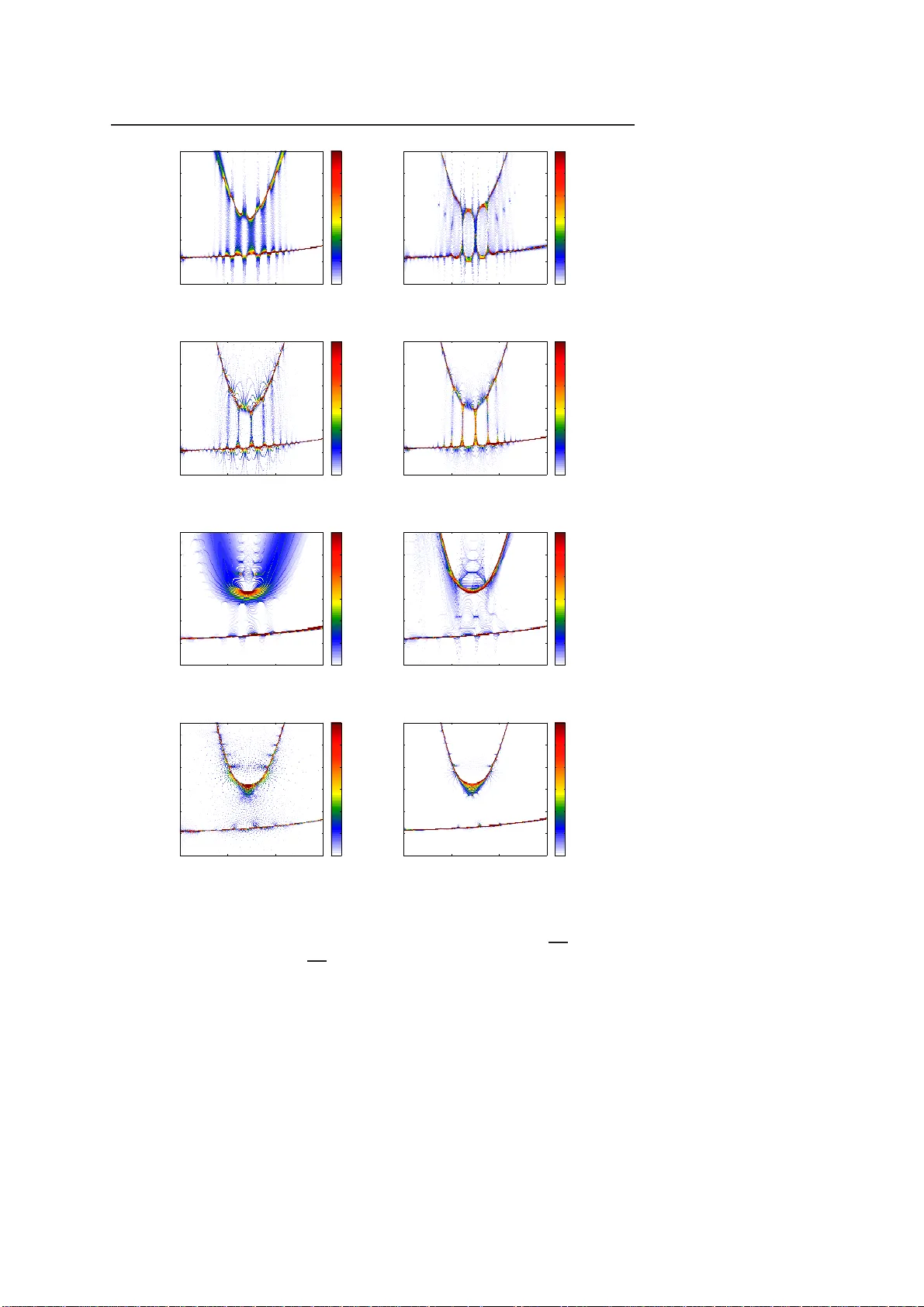
Noname man uscript No. (will be inserted b y the editor) En trop y-based time-v arying windo w width selection for nonlinear-t ype time-frequency analysis Y ae-Lin Sheu · Liang-Y an Hsu · Pi-T ai Chou · Hau-Tieng W u Receiv ed: date / Accepted: date Abstract W e prop ose a time-v arying optimal window width (TVOW W) scheme and an adaptive optimal windo w width (AO WW) s election sc heme to optimize the perfor mance of several nonlinear-t yp e time-freq ue nc y ana lyses, including the r eassignment metho d and its v ariatio ns. A window r endering the most con- centrated distribution in the time-frequency repres e n tation (TFR) is r egarded as the optimal windo w. The TV OWW selection s c heme is particula rly use- ful for sig nals that comprise fast-v arying instantaneous fr equencies and small sp ectral gaps. T o demonstr a te the efficacy of the metho d, in addition to a na lyz- ing synthetic sig nals, w e study an atomic time-v arying dip ole moment driven by t w o-color mid-infrar e d laser fields in attosecond physics and near -threshold harmonics of a h ydrog en atom in the strong laser field. Keyw ords Nonlinear -t yp e time-frequency analysis · Time-v arying optimal window width · Adaptive optimal window width · a tto s econd physics 1 In trodu ction Scient ists inv estigate nature by c o llecting diverse types of data. They then infer the underlying rules by mo deling and ana lyzing the recorded data . Time Y.-L. Sheu the Departmen t of Chemistry , National T aiwan Univ ersit y , T aip ei, T aiwan and the Depart- men t of Mathematics, Universit y of T oron to, M5S 2E4, T oronto, Canada L.-Y. Hsu the Department of Chemistry , N orth w estern Universit y , 60208, Ev anston, USA P .-T. Chou the Department of Chemistry , N ational T aiwan Univ ersity , T aip ei, T aiwan H.-T. W u the Departmen t of Math ematics, Universit y of T or onto, M5S 2E4, T oron to, Can ada and Mathematics D ivision, National Cen ter for Theoretical Sciences, T aip ei, T aiwan E-mail: hau wu@math.toron to.edu 2 Y ae-Lin Sheu et al. series is a commonly encountered da ta type. Its time- ev olving nature paves the w ay for scientists to access the sys tem’s dyna mics. Time- fr equency (TF) analysis is a p ow erful time series analysis tool, whic h captures nonstationary oscillator y dynamics and serves as a po rtal to the underlying system. During the pas t 70 years, several TF analy sis metho ds were developed [25], which can b e clas sified into three types: linear , quadratic, and nonlin- ear. Linear-type transfor ms, such as the short time F ourier transfor m (STFT) and t he con tin uous wa v elet transfor m (CWT), have b een widely studied. They a r e sub ject to the limitation of the uncer tain ty principle asso ciated w ith the CWT, o r the STFT [25, 26, 44]. Quadratic- t yp e transforms , such a s the Wigner-Ville distribution and Cohen clas s , could provide a mo r e adaptive analysis of the input signal. Howev er, they suffer from severe mo de mixing artifacts [25]. There are s ev eral no nlinear-type transforms including: the r eas- signment metho d (RM) [1 1, 3 ] and its v ariations, the TF by co nvex o ptimiza- tion (Tycoo n) [33], the Blasc hke decomp osition (BKD) [18, 19], the empirical mo de decomp osition (E MD) [30], the iterative filtering [17], the sparsification approach [29], the approximation appr oach [1 6], the TF jig s aw puzzle (TFJP) for the Ga bor tra nsform (GT) [32, 43], the non-s ta tionary GT (NSGT) [5], the matching pursuit [37], and sev eral others. The v a riations of RM include: the synchrosqueezing transform (SST) [22, 53], the sy nc hrosqueez e d w a ve pac ket transform [54], the synchrosqueezed S-transfor m [31], the seco nd-order SST [41], the concentration of fre q uency and time (ConceFT) [23], and the de- shap e SST [36]. While the approaches v ary from algorithm to algorithm, the common g oal of nonlinear-type tr ansforms is to o btain a “sharp ened” TF rep- resentation (TFR) that could pr ovide mo re accur ate dynamica l infor mation underlying the recorde d time series. W e refer int erested reader s to [23] for a more extensive literatur e sur vey a nd their applica tions. The nonlinear-type transfor ms can b e classified into tw o categ ories. The first ca tegory consists of transfor ms that do not requir e c ho osing a window, like the BKD, the E MD, and the Tyco on. While the EMD has been widely applied, its applicatio n to data analysis needs mor e attent ion due to its lack of mathematical foundation. The BKD, on the other hand, is solidly suppor ted by the complex a nalysis theor y . How ever, ther e ar e still several mathema tica l challenges left unsolv ed, and the applica tion of the BKD to data analysis is still in its infancy . The Tyco on is a s yn thesis-base d approa c h to es timate the TFR with the sparsity constra in t based on the conv ex optimization. The Tycoo n theoretically has the p otential to achiev e a sharp TFR, but it is currently compute-intensiv e. The seco nd categor y co nsists of transforms that dep end on a c hosen win- dow, which can b e cla s sified into t wo sub categor ies: reass ignmen t-type a nd non-reas s ignmen t-type. The rea ssignment-t ype subca tegory includes the RM and its v a riations, and the non-reass ignmen t-type sub catego ry inc ludes the other algo rithms. While different metho ds are sub ject to different limitations, they are all limited by the window sele ct ion problem. The question is: what is the optimal window when we analyze a given time series ? In the idea l situ- ation, the optimal windo w s hould b e univ ersal a nd always pr ovides the opti- TVO WW and AO WW 3 mal re s ults under some constr ain ts. How ever, it is widely believed that there probably is no optimal window due to the co mplica ted nonlinear it y hidden inside the natural signals. T o r esolve this is sue, different metho ds provide dif- ferent solutions. F or example, in the reassignment-t yp e transfor ms, we could theoretically prove that when the signa l and window sa tisfy some regula r it y conditions, the algo r ithms ar e adaptive to the signal, in the sens e that the depe ndence on the windo w is neg ligible; see, for example, [22, Theo rem 3.3]. How ev er, in practice, the situation mig h t b e more complicated. Therefore, the per formance of the alg orithm is not guar ant eed. Thus, how to determine the optimal window for nonlinear time series is a crucia l issue. In this pap er, we aim to alleviate this window selec tio n is s ue fo r the reassig nmen t-type transfo rms. W e co nsider the R´ enyi entropy to determine the o ptimal window. By applying the optimal window width, the TFR sharp- ness can b e enha nc e d while the reco nstruction r outine of the SST a nd its v a riations can b e preserved. W e sp ecifically consider a window that is optimal for a c hosen TF analysis , if the distribution of the asso cia ted TFR is highly concentrated. While there are several w ays to measure the dis tr ibution con- centration, we apply the R ´ enyi ent ropy [2 0, 6 , 45], which has b een shown to efficiently estimate the signal information conten t and complexity in the TFR. The article is org anized as follows. Section 2 summarizes t he background material, including the adaptive harmonic mo del (AHM) des cribing an oscilla- tory signal co mp osed of m ultiple co mponents, and several reass ignmen t-type TF analysis to ols tha t could b e applied to analyze such signals . Section 3 de- scrib es a s c heme to optimize the p erformance of the reas signment -type TF analyses b y window width selec tio n techniques. A compariso n of the prop osed scheme and some non-rea ssignment-t ype tr ansforms is also provided. Numeri- cal results a nd a n applica tio n to the attosecond physics are reported in Se c tio n 4. A conclusion is drawn in Section 5. 2 Bac kground In this section, we summarize the AHM to q ua n tify oscillator y signals, and re - view se veral r ecen tly pr opo sed TF analys is to ols suitable for ana lyzing signals satisfying the AHM. Wh ile the review could be extended to other r e assignment- t yp e transforms, suc h as the RM, the de-sha pe SST and the ConceFT, w e only review the SST 1 and the 2nd-order SST in this section. 2.1 Adaptive Harmonic Mo del The AHM aims to des cribe the time-v arying oscillatory dynamics in a giv en signal. Suppo s e that the s ignal x ( t ) is comp osed of finite K ≥ 1 oscillator y functions; that is , x ( t ) = P K k =1 f k ( t ), where f k is the k -th o scillatory function 1 The SST can b e defined also on the CWT [22], the S-transfor m [ 31], as well as other linear-type TF transforms [54]. Here we focus only on the SST defined on the STFT. 4 Y ae-Lin Sheu et al. and k = 1 , . . . , K . The k -th o scillatory function f k is co mp osed o f an amplitude mo dulation (AM) a k ( t ), which is positive, and a phas e function φ k ( t ), which is stric tly monotonically incre asing, s o that f k ( t ) = a k ( t ) cos(2 π φ k ( t )), for k = 1 , . . . , K . The φ ′ k ( t ) is thus p ositive and is regarded as the instantaneous frequency (IF) of the k -th os c illa tory function. In this study , we consider only real oscilla tory signals , s ince most time series we acquir e in the real world are real. While such a AHM describ es a s ig nal comp osed of multiple oscillato ry functions, it is to o gener al to work with a nd we need some constra in ts. Fix ǫ ≥ 0. Let the p ositive co nstan t c be the supremum of the v ariation of the IF function; that is, k φ ′′ k k ∞ ≤ c for k = 1 , . . . , K . It is also a ssumed that the v a riation o f the AM is controlled by the IF; that is, | a ′ k ( t ) | ≤ ǫφ ′ k ( t ) for all time t ∈ R and k = 1 , . . . , K . W e call an oscillatory function satisfying these constraints an in trinsic mo de t ype (IMT) function. Assume tha t the smalles t frequency gap b et ween tw o adja c e n t IMT comp onen ts is d , and d > 0 , for all time t ∈ R . That is, φ ′ k ( t ) − φ ′ k − 1 ( t ) > d , for k = 2 , . . . , K . In practice, we assume ǫ < 1 and is small eno ugh s o that the AM is slo wly v ary ing . The function satisfying the ab ov e conditions is said to be the generalize d AHM for the signal, and the constants ǫ, c, d are mo del parameters . 2.2 STFT The STFT of a tempered distr ibution x with respe ct to a c hosen windo w G in the Sch w artz s pa ce is defined by V G x ( u, η ) = Z ∞ −∞ x ( t ) G ( t − u ) e − i 2 πη ( t − u ) d t, (1) where u ∈ R is the time and η ∈ R + is the frequency . 2.3 SST The SST can b e embedded in different line a r-type trans fo rms, such as the CWT [22], the wa ve pa c ket [54] or the S- transform [31]. Here we only mention the SST em bedded in STFT due to the page limit. The SST with the resolution κ > 0 and the threshold γ ≥ 0 is defined by S G,κ,γ x ( u, ξ ) = Z A x,γ ( u ) V G x ( u, η ) 1 κ h  | ξ − ω γ x ( u, η ) | κ  d η , (2) where u ∈ R is the time, ξ > 0 is the frequency , A x,γ ( u ) :=  η ∈ R + :   V G x ( u, η )   ≥ γ  , h ( t ) = 1 √ π e − t 2 , κ > 0 and ω x ( u, η ) is the r e assignment rule : ω γ x ( u, η ) = ( − i∂ u V G x ( u,η ) 2 π V G x ( u,η ) when | V G x ( u, η ) | ≥ γ −∞ when | V G x ( u, η ) | < γ . (3) TVO WW and AO WW 5 The TFR determined b y the STFT is sha rpe ned by reassig ning its co ef- ficient at ( u, η ) to a different p oint ( u, ξ ) a ccording to the r e a ssignment rule. The SST is cle a rly nonlinear in nature. It is imp ortant to no te that the re- assignment r ule pr imarily dep ends on the phase information of the STFT, which contains the IF infor ma tion. According to the theor etical analys is in [53, 41], the TFR o f the SST is conce ntrated only on the IFs of a ll oscillatory comp onent s when the IF’s of IMT functions in x ( t ) are slowly v a rying. While the SST algorithm lo o k s co mplicated at the firs t glance, the idea un- derlying the algor ithm is intuit ive. T ake a harmonic function x ( t ) = Ae i 2 πξ 0 t int o acco un t. Cho ose the window function G that sa tisfies ˆ G is a real function and ˆ G ( ξ ) ≥ γ when ξ ∈ [ − ∆, ∆ ], wher e γ > 0 is chosen small enough and ∆ > 0. Note that x ( t ) is a n IMT function. The STFT of x ( t ) could b e dir ectly cal- culated b y the Plancheral theor em, and we hav e V G x ( u, η ) = A ˆ G ( η − ξ 0 ) e i 2 πξ 0 u . The information we hav e interest in a n oscillatory signal, the IF, is hidden in the phase of V G x ( u, η ). An in tuitive idea to obtain the IF in this case is first to a pply the loga r ithm function on V G x ( u, η ), next to divide it by i 2 π , and then to apply the deriv ative a ccording to u when | ˆ G ( η − ξ 0 ) | ≥ γ ; that is, d i 2 πd u  log( A ˆ G ( η − ξ 0 )) + i 2 π ξ 0 u  = ξ 0 . Clear ly , this oper ator is equiv alent to the reassig nmen t rule; that is, ∂ u log[ V G x ( u, η )] i 2 π = − i∂ u V G x ( u, η ) 2 π V G x ( u, η ) (4) when | ˆ G ( η − ξ 0 ) | ≥ γ . W e choose − i∂ u V G x ( u,η ) 2 π V G x ( u,η ) to estimate the IF s inc e we do not need to worry ab out the phase unwrapping problem when applying the lo garithm function to a complex function. T o contin ue, note that we hav e − i∂ u V G x ( u, η ) = 2 π ξ 0 V G x ( u, η ) by a direct calculatio n. Hence, ω γ x ( u, η ) = ξ 0 when η ∈ [ ξ 0 − ∆, ξ 0 + ∆ ] and ω γ x ( u, η ) = −∞ otherwise. F or this signal, we hav e A x,γ ( u ) = [ ξ 0 − ∆, ξ 0 + ∆ ], a nd the rea ssignment rule indicates that the IF is ξ 0 . Thus, the SST of x can then b e computed by the following equation: S G,κ,γ x ( u, ξ ) = e i 2 πξ 0 u Z ξ 0 + ∆ ξ 0 − ∆ ˆ G ( η − ξ 0 ) 1 κ 1 √ π e −| ξ − ξ 0 | 2 /κ 2 dη (5) = C e i 2 πξ 0 u 1 κ e −| ξ − ξ 0 | 2 /κ 2 , where C = 1 √ π R ∆ − ∆ ˆ G ( η ) dη ≈ 1 √ π G (0). Cle a rly , when κ is small, for each u , S G,κ,γ x ( u, ξ ) is concentrated around ξ 0 , which help a lle viate the smearing effect in the STFT caused by the uncertaint y pr inciple. 2.4 Second-Orde r SST When the IF is not slowly v ar ying, the sha rpe ning ability of the SST might be deteriorated. The 2nd-o rder SST resolves this pr oblem b y taking the seco nd order information in the phase of the STFT to co rrect the r eassignment r ule. 6 Y ae-Lin Sheu et al. The 2nd- order SST co uld b e viewed as a combination o f the SST and the RM – its sharpe ning ability is similar to that of the RM, a nd it allo ws us to reconstruct IMT f unctions like the SST. There ar e a t leas t tw o v ersions o f 2nd- order SST. W e discuss the v ertical SST (vSST) and the oblique SST (oSST) [41]. Both the vSST and the o SST depend o n the 2nd-order reass ig nmen t rule, which is a correctio n of the reass ignmen t rule ω γ x in (3): ˆ ω γ x ( u, η ) =  ω γ x ( u, η ) + c ( u, η )( u − ˆ t x ( u, η )) when ∂ η ˆ t x ( u, η ) 6 = 0 ω γ x ( u, η ) otherwise , (6) where u ∈ R is the time, η > 0 is the fre q uency , and ˆ t x ( u, η ) = u + i ∂ η V G x ( u, η ) V G x ( u, η ) and c ( u, η ) = ∂ t ω γ x ( u, η ) ∂ η ˆ t x ( u, η ) . (7) The vSST with the resolution κ > 0 and the threshold γ ≥ 0 is defined by v S G,κ,γ x ( u, ξ ) = Z A x,γ ( u ) V G x ( u, η ) 1 κ h  | ξ − ˆ ω γ x ( u, η ) | κ  d η ; (8) the oSST with the res olution κ > 0 and τ > 0 and thresho ld γ ≥ 0 is defined by oS G,κ,γ x ( u, ξ ) = Z Z V G x ( y , η ) e iπ (2 ξ − c ( y ,η )( τ − y ))( τ − y ) × 1 κ h  | ξ − ˆ ω γ x ( y , η ) | κ  1 τ h  | u − ˆ t x ( y , η ) | τ  d η d y . (9) Note that the vSST co uld be viewed as a direct g eneralization of the SST with the mo dified reas signment rule, while the oSST could b e viewed as a mixture of the SST a nd the RM. The r eader is refer red t o [41] for details of the 2nd-order SST and [8] for its theoretical analysis. 2.5 IMT function reconstr uction Each IMT function [2 2] can b e reconstruc ted from the SST, as well as the vSST, if the input signa l x ( t ) = P K k =1 x k ( t ) s atisfies the AHM. T ake the SST as an exa mple. Each IMT f unction x k = a k ( t ) cos(2 π φ k ( t )), k ∈ { 1 , ..., K } , can b e reconstructed by the following tw o steps. Fir st, ev aluate the “ complexification” of the k -th IMT function b y ˆ x C k ( t ) = 1 G (0) Z ˆ Z k ( t ) ˜ S κ,γ G,x ( t, ξ )d ξ , (10) where ˆ Z k ( t ) = [ ˆ φ ′ k ( t ) − ǫ 1 / 3 , ˆ φ ′ k ( t ) + ǫ 1 / 3 ] and ˆ φ ′ k ( t ) is the estimated IF of the k-th IMT function, which can be obtained b y the r idge e xtraction a lgorithm [12, 9, 38]. Then, the k -th IMT function is then extracted by ˆ x k ( t ) = ℜ ˆ x C k ( t ) , (11) TVO WW and AO WW 7 where ℜ is the ope r ator ta king the rea l par t of the input complex v alue. The reconstructio n formula (10) could s erve as an appro ach to obtain the co mplex form o f a real signal. This pr oper t y is imp ortant since, in general, ev aluating the c o mplex form of an IMT function is a nontrivial issue. It is opted that there are several constra in ts for the sp ectra o f a k ( t ) and cos(2 π φ k ( t )) in order to successfully obtain the imaginary counterpart o f x k ( t ) a nd a k ( t ) sin(2 π φ k ( t )) via the Hilbert transform. W e refer the reader with in terest to [7, 40] for details. 3 Time-V arying Opti mal Windo w Widths It has been well-kno wn that a short window is helpful for analyzing a signa l with fast-v arying IF comp onents. O n the o ther hand, for sig na ls w ith tw o IMT functions with close IFs, the window should b e long enough to av oid sp ectra l ov erlaps. An “optimal” window should pro vide a balance b etw een these tw o facts. How ever, the uncertain ty principle [26, 44] s uggests that th e b enefits of a short and a long windo w width cannot be attained simultaneously . In this regar d, w e need a metho d to choos e a pr oper window width dynamically to balance on bo th e nds . Several attempts have b een prop osed in the literature to ba la nce b etw een different window bandwidths. F or exa mple, in [3 2, 4 3], the TFJP w as prop osed to select the o ptimal window for the GT based on the R´ enyi en tropy [20]; in [4], the NSGT depends o n a frame asso cia ted with a non-unifor m gr id on the TF plane, which comes from the information provided by the signal. The frame could b e viewed as the “optimal window” for the GT. These approaches hav e bee n shown to be helpful in the audio pro cessing [32], fo r example, the b eat tracking pr oblem [2 8]. In general, these approaches could be unders too d as the TF tiling or a dictionar y lea rning pro ble m – for a chosen redundancy , how to provide the b est tiling of the TF plane, o r to c ho o se the optimal frame, so that the TF representation is “optimal” based on a c hosen cr iter ion, for example, the minimal ℓ 1 norm [24] or the minimal R´ en yi entropy . The reass ig nmen t-type transforms could be viewed as an approach to so lv e the dictionary lea rning pro blem by taking the phase of the STFT in to account. Note tha t the STFT could be viewed as ev aluating the co efficients of a sig na l asso ciated w ith a n infinitely redundant dictionary D = { G ( t − · ) e i 2 πξ t } t ∈ R ,ξ ∈ R + , (12) where G is the chosen window. Dire ctly determining the o ptimal fra me out of D is not an easy tas k. Instead of determining the optimal fra me, the reassig nmen t rule used in the RM and the SST and its v ariations could b e viewed as an alternative to approximate the optimal frame out of D . Note that in the SST (2), the vSST (8), and the oSST (9), the coefficients of the STFT are moved to a new lo catio n based on the r e assignment r ule. In this sense, nonlinear -t yp e TF analysis could b e viewed as ev aluating the co efficient s of an appr o ximated optimal frame. W e mention that this viewpoint has been taken in to accoun t to design the T yco on alg orithm [33]. Theoretically , if the signal sa tisfies the 8 Y ae-Lin Sheu et al. AHM model, it has been shown that the reassig nmen t rule could lead to the optimal fra me [1 2, 2 2, 4 1]. How ever, due to the lack of knowledge of the mo del parameters , like ǫ, c, d of a g iv en signal, the reassignment rule, and hence the TFR, might b e influence d by the interaction of the chosen w indow and the time-v a rying AM and IF, and the ov erlap o f sp ectra o f different o scillatory comp onent s. In practice, although we hav e a rule of th umb of ho w to c hoo se the window based on the a pr iori knowledge of the signal, the reas signment rule might deviate from the optimal frame. In order to reso lve this issue, we prop ose an a daptive wa y to determine the o ptimal window for the reassignment-t yp e transforms. This a pproach can be vie wed as corr ecting the approximated optimal frame deter mined by the reassig nmen t rule. A window is regar ded as optimal for a chosen reassignment- t yp e TF ana lysis if it provides the most co ncen trated TFR. Since the IF a nd AM o f each IMT function may v ary from time to time, a single windo w optimal for the e ntire signal mig h t not b e suitable. Therefore, the no tion o f the optimal window for a chosen TF analy s is sho uld be lo c al . F o r example, for each time, we determine an optimal window. In gener al, finding the optimal window is a difficult task. In s tatistics, the problem is commonly reduced to the window b andwidth sele ction problem [52]. In this work, we simplify the window selection problem to the window bandwidth selection problem. T o further simplify the discus sion, we consider the Gaussian window, that is, G ( t ) = g σ ( t ) := 1 √ 2 π σ e − t 2 / (2 σ 2 ) , (13) where σ > 0 is the b andwi dth of the window. In this ca se, the STFT is the same as the GT. In this sectio n, for a chosen TF analysis with the Gaussian window (13), we descr ib e a time-v arying o ptimal window width ( TVO WW) selec tio n scheme a nd an ada ptiv e optimal window width (A OWW) selection s c heme to compute a s eries of local optimal windo w widths. W e men tion that a lthough we fo cus o n the window bandwidth selection problem with the Gaussia n window, the discussion b elow could be dir ectly g eneralized to other window functions, or even multiple window functions. 3.1 The TV OWW and the AO WW s election s c hemes First s e lect a reass ig nmen t-type transfo rm, for example, the SST. The TVO WW selection sc heme ev alua tes the lo cal windo w width b y iterating the following steps for each time u ∈ R : 1. Ev aluate the distr ibution concentration of the TFR o n [ u − b , u + b ] × R + , where b ≥ 0 deter mines the size of the neighborho o d, b y a chosen distribution concentration measure, denoted as C σ,b ( u ). 2. The lo cal optimal window width at the time instant u is determined by ˜ σ b ( u ) := arg min σ> 0 C σ,b ( u ) . (14) TVO WW and AO WW 9 3. Apply the windo w width ˜ σ b ( u ) to ev aluate the TFR of the signal x ( t ) at time u . The prop osed scheme co uld b e dir ectly a pplied to other TF analys es, such as the STFT, the 2nd-o rder SST or other nonlinear TF analy s es. When b = ∞ , ˜ σ b is a c o nstant v alue a nd the SST is reduced to the orig inal SST with one window width, which is c hosen to optimize the selected measure of distribution concentration. W e reg ard this sp ecial case the glob al optimal window width (GOWW ). The AO WW selection scheme ev aluates the lo cal window width via iterat- ing the following steps for a given pair of time and frequency , ( u, ξ ). 1. Ev aluate the distr ibution concentration of the TFR o n [ u − b , u + b ] × [max { 0 , ξ − b F } , ξ + b F ], where b ≥ 0 determines the s ize of the neighbo rho od and b F > 0 determines the size of the neighborho o d in the frequency axis , by a c hosen distribution concentration measure, deno ted a s C σ,b,b F ( u, ξ ). 2. The lo cal optimal window width at the time instant u is determined by ˜ σ b,b F ( u, ξ ) := argmin σ> 0 C σ,b,b F ( u, ξ ) . (15) 3. Apply the window width ˜ σ b,b F ( u, ξ ) to e v aluate the TFR of the sig na l x ( t ) at time u a nd frequency ξ . While the AO WW could pr o vide a shar per TFR, compared w ith the TVOWW , the c o mputational burden of the AO WW selection scheme is grea tly incr eased. F ur thermore, for a given time u , since the window width v ar ies for different frequencies, the r econstruction formula (10) ca nnot b e a pplied. W e mention that t he ab ov e algorithm can be easily generalized to selecting m ultiple win- dow functions. Ther eb y , different windows ca n b e taken in to account in the optimization (1 4) o r (15), so that the optimal window function a nd its cor - resp onding optimal window width are selected. Since the m ultiple window selection is out of the scop e of this work, we will study it in the future work. 3.2 R´ en yi entropy The information en tropy is a common measure to estimate the dispersio n o f an information co n tent. By viewing the TFR a t each time as a probability density function, a larg er entropy indicates a less distr ibuted concentration o f the TFR. In th is study , we adopt the R´ enyi entrop y to meas ur e the distribution concentration of a TFR [6]. The α - R ´ enyi entropy of a non-zero function p , where α > 0 , is defined as R α ( p ) := 1 1 − α log 2  k p k 2 α k p k 2  2 α , (16) where k p k α := ( R | p ( x ) | α dx ) 1 /α for 0 < α < ∞ . Note that when α < 1, k · k α is not a norm but a quasi-nor m. It is w ell-known that the larger the R´ en yi ent ropy is, the less concent rated the distribution is [3 2, 4 8]. That is to say , a 10 Y ae-Lin Sheu et al. window width providing the least R´ enyi ent ropy is r egarded as the optimal window width. Note that when α → 0, the R ´ enyi entropy gives the ℓ 0 norm information of the signa l; whe n α → 1, the Shannon entropy is recovered; and when α → 1 / 2, we obtain the information of the commo nly used ratio norm ℓ 1 /ℓ 2 . In g eneral, α > 2 is recommended for TFR measur es [48] and w e chose α = 2 . 4 in this study . In practice, we notice that the results are insensitive within a certain range of α v alue s ( α > 0). Denote the T FR o f a chosen TF analysis P defined on R × R + . The TFR distribution is considered the most concentrated if its corr espo nding R´ en yi ent ropy is minimized. W e th us define the measure o f distribution co ncen tration in the TV OWW selection scheme as C σ,b ( u ) := 1 1 − α log 2 RR I u | R ( t, ξ ) | 2 α d t d ξ  R R I u | R ( t, ξ ) | 2 d t d ξ  α , (17) where u ∈ R and I u := [ u − b, u + b ] × [0 , ∞ ). Similar ly , the distribution concentration measure in the AO WW s e le ction scheme is defined as C σ,b,b F ( u, ξ ) := 1 1 − α log 2 RR J u,ξ | R ( t, ξ ) | 2 α d t d ξ  RR J u,ξ | R ( t, ξ ) | 2 d t d ξ  α , (18) where u ∈ R , ξ ∈ R + , and J u,ξ := [ u − b, u + b ] × [max { 0 , ξ − b F } , ξ + b F ]. 4 Results and Discussio ns W e start the demonstr ation of the prop osed the TVO WW and the AO WW selection schemes by analyzing a synth etic data. W e then show the result of analyzing the laser-driven atomic dip ole momen t, and discuss the performa nc e of the pro pose d scheme. In this sectio n, for the SST and the 2nd- o rder SST, the numerical v alue of κ a nd τ are selected to b e sma ll enough s o that 1 κ h ( · κ ) and 1 τ h ( · τ ) a re both implemen ted as discretized Dirac meas ur es. The γ v alue is fixed at 10 − 6 % o f the mea n squa re energy of the sig nal x ( t ) under analysis . 4.1 Synthet ic Signal Consider a mult icomp onent sig na l given by x ( t ) = x 1 ( t ) + x 2 ( t ) + x 3 ( t ) , (19) where the signal comp onents are: x 1 ( t ) = cos(2 π φ 1 ( t )) χ [ −∞ , 20] ( t ) x 2 ( t ) = cos(2 π φ 2 ( t )) χ [ −∞ , 13 . 6] ( t ) x 3 ( t ) = cos(2 π φ 3 ( t )) χ [17 . 5 , ∞ ] ( t ) , TVO WW and AO WW 11 where χ I is the indicator function suppo rted on I ⊂ R a nd φ 1 ( t ) = 1 . 33 t − 5 + 3 t φ 2 ( t ) = − 0 . 04 37( t − 5 ) 4 + 0 . 5( t − 5) 3 + 0 . 25( t − 5) 2 + 5 t φ 3 ( t ) = − 2 . 7 3 . 5 cos (3 . 5 t ) + 0 . 85( t − 15) 2 + 0 . 5 t. The corre s ponding IFs are φ ′ 1 ( t ) = (ln 1 . 3 3) 1 . 33 t − 5 +3, φ ′ 2 ( t ) = − 0 . 175( t − 5) 3 + 1 . 5( t − 5) 2 + 0 . 5( t − 5) + 5, a nd φ ′ 3 ( t ) = 2 . 7sin 3 . 5 t + 1 . 7( t − 15) + 0 . 5 . The obs e r ved signal Y ( t ) = x ( t ) + λΦ ( t ), where Φ is the white Gaussian noise with mean 0 and standard deviation (std) 1 , and the λ v alue ( λ > 0) is chosen so tha t the signal-to- noise ratio (SNR), defined as 20 log std( x ( t )) λ , is 15 dB. Y ( t ) is sa mpled at 60 Hz from the 0-th to the 25 -th second (s). W e select the optimal window width σ from a se t of candida te bandwidths, { 1 1 / 720 , 31 / 720 . . . , 501 / 72 0 } s . 4.1.1 TFR wi th the GOWW W e first s ho w the limitation of using the GOWW selection scheme for the SST. In other w ords, w e run the o ptimal windo w selection sc heme with b = ∞ , resulting in the GO WW of 7 1 / 720 s. Fig. 1(a) demonstrates that the SST with the GOWW can capture the o scillatory dyna mics. Nevertheless, while a small window width is required to reduce the R´ enyi entrop y in the TFR, it results in the evident interference pattern b etw een the neighboring IF comp onents. F or example, the sp ectral ga p (diff erences betw een the a djacen t IF comp o nen ts) at the 5-th s (i.e., φ ′ 1 (5) and φ ′ 2 (5)) is 1 . 8 Hz, a nd a strong interference pattern is o bserved at the 5-th s . According to Definitions 3.1 a nd 3 .2 in [2 2], the window width, measured by the full width at half maxim um (FWHM), whic h is defined as 2 √ 2 ln 2 ˜ σ b , s hould b e at least 1 / 1 . 8 ≈ 0 . 55 s in o r der to separate the tw o neighboring comp onents in the AHM. Her e, the FWHM of the GOWW is 0 . 23 s, which is insufficient and leads to the interference pa ttern. Similar int erference patterns ca n be obs e r ved at times 1 3 . 6 s , a nd 18 . 5 s, where sp ectra l gaps are approximately 3 Hz and 7 Hz, r e s pectively . It is clear that a larger sp ectral gap results in a less coupled interaction b et ween the IF components. In summary , since the optimal window is chosen globally , the loca l details ma y not b e refined ev en if the ov erall sha rpness of the TFR is increa sed. 4.1.2 TFR wi th the TVO WW W e next demons trate that the propos ed TVO WW se lection scheme can further improv e the TFR qualit y . T o reduce the computation capacity , w e ev aluate the lo cal optimal window width every 0 . 25 s in a neighbor hoo d with a width o f 2 b = 0 . 3 3 s. The neig h b orho o d size is found to be inse nsitiv e to the final result. While a sma ll v alue is favorable, the width of the ne ig h b orho o d should be greater than the sampling pe r io d [27]. Subsequently , a linear in terpo lation is applied to the s amples of the TVO WWs such that there is an o ptima l window for each time insta n t in the signa l interv a l. The TFR of the SST with the 12 Y ae-Lin Sheu et al. TV OWW is presented in Fig. 1(b) and its co mparison w ith the true IFs is display ed in Fig. 1(c). It is clearly shown that the coupling artifact betw een closing IF c ompone nts is eliminated, par ticula rly at the 5th s, as well as at the 13 . 6 , and 18 . 5 s. The IF co mponents in the TFR with an improv ed quality approaches the ideal IF comp onents, as in Fig . 1(c). W e further display the corres p onding TV OW W along with t he sp ectral gap in Fig. 1(d). According to this figur e, the window widths become large at the closing times 5 s , 13 . 6 s, and 18 . 5 s to separate the different IF compo nen ts. Note that at time 5 s , the larg est window width is ˜ σ b = 345 720 = 0 . 48 s, corresp onding to a FWHM of 1 . 08 s, which is large r than 0 . 55 s. Time (Sec) Frequency (Hz) 5 10 15 20 25 0 5 10 15 20 25 0 1 2 3 4 5 6 (a) SST w i th the GOW W Time (Sec) Frequency (Hz) 5 10 15 20 25 0 5 10 15 20 25 0 1 2 3 4 5 6 (b) SST with TVO WW Time (Sec) Frequency (Hz) x 1 (t) x 2 (t) x 3 (t) 0 5 10 15 20 25 0 5 10 15 20 25 0 2 4 6 8 10 (c) Comparison with ideal IFs 5 10 15 20 25 0 10 20 Spectral gap Hz 5 10 15 20 25 0 0.1 0.2 0.3 0.4 0.5 TVOWW Time (Sec) Sec (d) Spectral gap and the TVO WW Fig. 1: (a) The TFR of the SST with the GO WW. (b) The TFR of the SST with the TVO WW. (c) The true IFs (blue: x 1 ( t ); ma gen ta: x 2 ( t ); r ed: x 3 ( t )) a r e sup e rimpo s ed on the TFR of the SST with the TVO WW. Note that the r a nge of the colorba r is incr e ased for th e c o mparison. (d) The spectra l gap (upper panel) and the cor r esp o nding TV OWW (low er panel). It is clea r that when the sp ectral gap is sma ll, a lo nger window is needed. The TFR v a lues are normalized by the z-sco r e. TVO WW and AO WW 13 4.1.3 Ne c essity of Sele cting a Pr op er Windo w Width In this subsection, w e accen tuate that while the 2nd-or der SST and the RM could provide a sharp er TFR co mpared with the SST, the impact of the win- dow width is not neg ligible. W e demonstrate the TFR o f the syn thetic signal (19) analyzed by the 2 nd- order SST and the RM in Fig. 2 and Fig. 3. In b oth figures no noise is inv olved. While the 2nd-order SST and the RM can mit igate the limitation of the SST caused b y the fas t-v ar ying IF components, witho ut a prop er choice of the window width, the 2nd-o rder SST and the RM could fail. Figure 2 shows that a la rge window width is required to separa te the t w o comp onent s with clos ing IFs. The (a)-(d) in Fig . 2 are TFRs using a small window width 111 720 s, which is the GOWW o f the vSST. The coupling artifact betw een the t wo comp onents ca used by the s ma ll width for the a ll transfor ms is ev ident. As mentioned in previous s e ctions, the coupling artifact can be greatly diminished by increasing the window width. In (d)-(h) in Fig. 2, we choose the window width as 345 720 s, which is the largest TVO WW for the SST. F o r all TFRs, the tw o IF comp onents are clearly sepa r ated, particularly in the RM result Fig. 2(h). Figure 3 shows that a small window width is requir ed to capture the v a riation in an oscillating IF comp onent. Note tha t the small w indow width is 111 720 s and the larg e window width is 251 720 s. A small window width pro vides a fine tempo ral resolution, whic h allows us to extra ct the dynamical information of an IF comp onent ((a)-(d) in Figure 3), while a lar g e w indow width cause s ambiguit y in temp oral directio n ((e)-(h) in Figure 3). In summary , a prop er windo w width is a prerequisite to obtain the a c curate IF infor mation in the TFR in spite of the fa ct that the con ven tional r eassign- men t rule in the RM and high-or der reassig nmen t rules in the 2nd-order SST can cop e with the fast-v a rying IF co mponents efficiently . 4.1.4 R e c onstruction Err or A nalysis Finally , to qua ntify the improv ement of the TFR by taking the TV OWW in to account, we ev aluate the normalized ro ot-mean-sq ua re deviatio n (RMSD) b y comparing the reco nstructed signa l comp onents, the IF, and the AM with corres p onding true answers. The normalized RMSD for the ev aluation comp onent ˆ f i , where i = 1, 2, and 3, is given as normalized RMSD( ˆ f i ) = k ˆ f 2 i ( t ) − f 2 i ( t ) k L 2 | f i, max − f i, min | , (20) where f i, max and f i, min are the maximum and min imum v alues o f f i , respec- tively . Here ˆ f i can represent the rec onstructed sig na l comp onent ˆ x i , the re- constructed IF and the reconstructed AM from the TFR. 14 Y ae-Lin Sheu et al. In addition to the noiseless co ndition, we c o mpute the nor malized RMSD for SNR of 1 5 a nd 10 dB for 25 trials, and r epo rt the mean and the standar d deviation of the normalized RMSD. The results for the reco nstruction per formance, the reconstructed IF, and the reconstr ucted AM for ea c h c o mponent ar e pres en ted in Fig. 4, 5, and 6, r espectively . The IF compo nen ts are estimated by ev alua ting the ce n ter of mass o f the TFR. The AM co mponents a r e e x tracted from the env elope o f the reconstructed signal comp onents. Note that the error v aries for different metho ds to co mpute the AM c o mponents. The results confirm the b enefit of the TV OWW selection scheme, particu- larly for the c ompone nts x 1 ( t ) and x 2 ( t ). F or x 3 ( t ), the er rors of the GOWW and the TV O WW selection sc hemes are similar, since th is signal compo nen t is less coupled with the others. The results for the reconstr ucted IF and the recons tructed AM for ea c h comp onent a re pr esent ed in Figure 5 and 6, res pectively . The IF comp o- nent s a re estimated by ev aluating the center of mass o f the TFR. The AM comp onent s are extracted from the env elop e of the r econstructed signal com- po nen t. Note that the error v aries for differen t methods to compute the AM comp onent s. Although not shown in the pap er due to the pag e limit, w e men tion tha t the TVO WW selection technique ca n b e applied to the 2nd-SST and o ther v a riations o f the SST t o improv e the re c o nstruction quality . 4.1.5 T owar d an Optimal ly Conc entr ate d TFR – A OWW W e demonstra te that the AO WW selection scheme can achiev e a more con- centrated TFR by considering the optimal window width in bo th time and frequency axes. F or the exa mple of the synthetic s ignal, we set 2 b F = 1 . 6 Hz and ev aluate the lo cal o ptimal window width ev ery 1 . 4 Hz. The TFR results for the SST and the vSST using the AO WW s election sc heme are present ed in Fig. 7. B y comparing Fig.7(a) with Fig.1(b), we found that the TFR is sharp ened using the AO WW s election scheme, at the exp ense of significa n tly increased computation a nd the lo st of the inv erse routine to reco nstruct ea c h IMT comp onent. Moreover, the T FR of the vSST with the AO WW (Fig.7(b)) and that with the TV OWW is similar. 4.1.6 The Influenc e of Par ameters in the GOWW, the TV O WW and the AO WW Sele ction Schemes W e mention that the optimal α v alue c hosen for the Renyi e n tropy mig h t depe nd on the application. F o r a s pecific application, we co uld further optimize α , and it might dep end on par ameters s uc h as the sampling rate, freque nc y - axis and time-axis discretization, and the parameter b and b F . In this subsec tion we show that the GOWW, the TVOWW and the AOW W selection sc hemes are not sensitive to these parameters. T able 1 presen ts the normalized RMSD of the r e constructed co mponents for thr ee differ en t α , which TVO WW and AO WW 15 T able 1 Comp onen t reconstruction errors for three differen t v alues of α in the GO WW and the TVOW W selection sche mes. Here b and b F are fixed. α = 2 α = 2 . 4 α = 2 . 8 x 1 ( t ) GOWW 0 . 1177 0 . 1177 0 . 1177 TVO WW 0 . 0357 0 . 0359 0 . 0353 x 2 ( t ) GOWW 0 . 1152 0 . 1152 0 . 1152 TVO WW 0 . 0288 0 . 0287 0 . 0280 x 3 ( t ) GOWW 0 . 0202 0 . 0202 0 . 0202 TVO WW 0 . 0210 0 . 0213 0 . 0213 T able 2 Component reconstruction err ors for three different v alues of b in the TVO WW selection scheme. Here α and b F are fixed. b = 0 . 08 s b = 0 . 17 s b = 0 . 25 s x 1 ( t ) 0 . 0354 0 . 0358 0 . 039 8 x 2 ( t ) 0 . 0288 0 . 0294 0 . 034 2 x 3 ( t ) 0 . 0199 0 . 0200 0 . 020 0 T able 3 Instan taneous fr equency reconstruction error wi th three different v alues of b F in the AO WW selection scheme. Here α and b are fixed. b F = 0 . 6 Hz b F = 0 . 8 Hz b F = 1 . 0 Hz x 1 ( t ) 0 . 0184 0 . 0170 0 . 0150 x 2 ( t ) 3 . 29 × 10 − 4 2 . 72 × 10 − 4 2 . 66 × 10 − 4 x 3 ( t ) 0 . 0056 0 . 0049 0 . 0050 are 2, 2 . 4, and 2 . 8. Here b a nd b F are fixed. T able 2 pre s en ts the normaliz e d RMSD of the reconstructed comp onents for three different b , which a re 0 . 8 s, 0 . 17 s, a nd 0 . 25 s. Here α a nd b F are fixed. Since no r econstruction ro utine is av a ilable for the A OWW, the ev aluation of the dep endence of the A OW W on the chosen par ameters is based o n the devia tion of the IF co mponents via ridge e x traction. T able 3 presents the normaliz e d RMSD of the reconstructed IF comp onents for three different b F , which are 0 . 6 Hz, 0 . 8 Hz, and 1 Hz. Here α and b a re fixed. Here the loc a l o ptimal windo w widt h is ev aluated every 1 Hz. The s e r esults pr ovide the evidence that the GOWW, the TV OWW, and the A OWW selection schemes ar e stable to thre e ma jor parameter s α , b , and b F . 4.2 Application to A ttosecond Physics During the past decade, r eal-time observ ation and direct control of electronic motion in a toms, molecules, nano structures and solids have been achiev ed due to a dv ent in the synthesis o f attoseco nd pulses [34]. In gener al, an isolated attosecond pulse is cr e ated b y the sup erp osition of a bro a dband sup erco n tin- uum in high-order harmonic g eneration driven b y high-in tensit y femtosecond laser pulses [13]. T o date, an isolated attosecond pulse as short as 67 attosec- onds has been rep orted [55]. T o synthesize shor ter attosecond pulses, a b etter understanding of the underlying physical mechanism is needed. The ph ysical mechanism of the synthesis of a ttosecond pulses can b e under stoo d by ana- lyzing the electron dipo le mo men t oscillation induced by an applied laser field 16 Y ae-Lin Sheu et al. via the TF ana lysis. In the previous litera tur e [1 , 2, 14 , 35, 39, 42, 47, 50, 51], the linear-type transfor ms bas ed on s hort window widths have b een adopted and the results are consistent with the classical tra jecto ry simulations [21]. How- ever, ther e is no disc us sion on how and why small windows a re chosen in t he field of attosecond ph ysics. T o clarify this issue, we study the electron dip ole mo men t in atomic hy- drogen evoked b y an optimally shap ed laser wa v eform that can g e nerate an isolated 21 attosecond pulse [15]. Such a laser pr o file can greatly extend the high-order harmonics up to 900 harmonics within a sho r t time interv a l, sug - gesting fast-v arying IF comp onents. The time-dep endent dip ole momen t in the acceleratio n for m is computed by solving a three-dimensional time-dep endent Schr¨ o dinger equation in th e framework of the time- dependent generaliz e d pseu- dosp ectral (TDGPS) metho d within the elec tr ic dipo le approximation [49]. The TDGPS metho d gives accurate orbital ener gies and has b een employed in the strong field ph ysics as well a s attosecond science. The sim ulation details are referred to [15]. W e then co mpute the R´ en yi entropy for a series of window widths, ra nging from 0 . 25 ato mic units (a.u.) to 8 . 3 3 a.u. W e apply the TV OWW se le c tion scheme with a neighbor ho o d size of 2 b = 1 0 a.u., resulting in Fig. 8. Fig. 8 indicates tha t there ar e three emissions taking place. The cutoffs o f the first and third emissions are located at around the 50 0th o rder, and the sec ond emiss ion reaches the 900th order . The branches o n the TFR nearly coincide with the classical tra jector ies r epo rted in the previous literature [15]. F o r comparison purp oses, enla rged details of the seco nd emission with the GOWW and the TV OWW ar e display ed in Fig. 9. It is obs erved that at ar ound 0 . 43 laser cycles (1 laser cycle = 275 . 77 a.u.), the bra nc h indicated by the blue arr ow in Fig. 9(b) corr espo nding to the lo ng tra jectory quant um path has the stro ngest int ensity and consists of the most harmonics. While the branch indicated by the red arr ow dies out after 0 . 35 las er c y cles in the TFR o f the SST with the GOWW (Fig. 9(a)), it is r evealed b y the r esult with the TV OWW (Fig. 9(b)) that the short tra jectory quan tum path also has an influence on the high order harmonic emission. These high o rder har monics occ ur a lmost simultaneously , which is a prerequisite of a dep endable attosecond pulse. In the sec ond ex ample, we demonstrate that the A OWW s e lection scheme is beneficia l to distinguish the near-threshold harmonics in the TF repres en- tation of a hydrogen atom in the s tr ong laser field . Figure 10 shows the TF r epresentations for HHG genera ted b y a mo nochromatic laser field with a w av elength o f 800 nm and an in tensit y of 5 × 10 13 W/cm 2 . The laser field profile is describ ed b y sin 2 ( π t/ ( nT )), wher e n = 40 is the pulse length mea- sured in optica l cy c les ( T = 2 π /ω 0 ), and ω 0 is fundament al angular frequency of the laser wav elength. (The definit ion of the laser field profile and the s im- ulation details can b e found in [47, 46].) The laser parameter s c orresp ond to the Keldysh par a meter γ K = 1 . 51 [10, 47], indicating that the main dynamic mechanism is the multip hoton io niz a tion proc ess. Generally sp eaking, γ K ≫ 1 and γ K ≪ 1 corr espo nd to the multiphoton ioniza tion r egime and the tun- neling ionization regime, respectively . Figure 10(a) presents the result of the TVO WW and AO WW 17 synchrosqueezed Mor let wa velet transform with a scaling par ameter τ = 6 , and in Fig. 10(b) the AO WW selection sc heme is applied. Due to the adv an- tage of m ultiresolution, the sy nc hrosqueez e d Morlet wav elet transfor m [35, 47] can clearly describ e the b elow-threshold harmonics (from the 1st to the 5 th harmonics), and the chirp-like dynamics in the ab ov e-thresho ld region. How- ever, in the near-threshold regio n (The ionization thr e shold in this case is the 8 . 78th har monic.), the harmonics (i.e., from the 7th to the 11th harmo nics) are coupled and ambiguous. After applying the AO WW selection s cheme with a neighborho o d size of 2 b = 0 . 24 T and 2 b F = 0 . 46 ω 0 , the near -threshold har - monics in Fig . 10(b) ar e clear ly depicted in the TFR. The se c ond exa mple indicates that the AOW W selection scheme ma y be a pplied to other atomic systems such as the Cs atom [35]. 4.3 A compariso n with other metho ds The prop osed TVO WW a nd the A OWW selection sc hemes ha ve s imilarities with some no n-reassignment-t yp e TF analysis metho ds. F or example, in the sparsificatio n approach [29], when the signal satisfies the r egularity conditions of the AHM, a dictionary des ign and a sparsity based optimization lead to the desired time-v a rying s p ectra l informatio n and signal decomp osition. How ever, it is not cle ar how to achieve the o ptimal dictio na ry desig n, a nd the optimiza- tion step in the sparsification c ould be compute-in tensive if the dictionary is chosen improp erly . T o hav e a parallel c o mparison with the reassig nmen t-type transforms, note that the dictionary in the rea ssignment-t ype transfo r ms, for example, D in (12), is infinitely redundant. The “o ptimal” frame is not chosen by any direct optimization pro cedure. Instea d, the reassignment rule provides an approximation of the optimal fr a mes. When combined with the TVO WW or the A OWW selection scheme, we get the optimal frame ov er an infinitely redundant dictionar y . In this sense, when combined with the TVO WW o r the A OWW, the reassignment-t yp e trans forms could be viewed a s a v ariation of the sparsificatio n approa c h. The Tycoon [33], o n the other hand, could b e viewed a s a TF ana ly sis techn ique base d on the convex o ptimization from the synthesis viewp oint [4]. In this appr o ach, we do not design a dictionary o r choose a window. Instea d, we need to determine s ome fundament al quantities that a “go o d” TFR sho uld satisfy , and then dir ectly find this go o d TFR by o ptimizing a functional cap- turing the deter mined fundamental quantit ies. Since the TFR determined by the SST could a pproximate th e consider ed functional [22, 33], the co m bination of the TVO WW or the AOW W and the SST and its v a riations could be viewed as a relaxation of the Tycoon. In the TFJP [3 2], we first fix a TF plane tiling. F or e ach blo ck in the TF plane tiling, the optimal window for the GT is then selected ba sed on the R ´ enyi en tropy . While it leads to a shar per TFR, the “ uncertaint y” still exists. F ur thermore, since the TF plane tiling is not uniformly dis tr ibuted, the signa l decomp osition ability is limited. While the SST and its v ariations combined 18 Y ae-Lin Sheu et al. with the TVO WW or the AO WW sele ction schemes could b e viewed a s a v a riation of the TFJP in the sense o f “window selection”, we men tion that the TFJP a nd frame-base d metho ds a re different in essence. Specific a lly , TFJP is not s p ecifically designed fo r sums of frequency mo dulated sig nals but for a more general signal, so the application fields of the TFJP are different . 5 Conclusions In this study , we prop ose tw o optimal window width s e lection schemes, namely , the TV OWW a nd the A O WW selection tec hniques, to optimize the concen- tration of the TFR deter mined by a chosen TF analysis . The R ´ enyi en tropy is applied to determine the concen tration of the TFR. In addition to sho wing the per formance of the propose d sc heme in a syn thetic s ig nal, we show p otent ial applications of this method to a tto s econd physics. W e believe that this work can serve as a corner stone in ultrafast dynamics in atoms and molecules to uncov er new physics. 6 Ac kno wledgemen t Hau-tieng W u acknowledges the supp ort of Slo a n Research F ellow FR-2015- 65363 a nd P rofessor Br uno T orresa ni and P rofessor Matthieu Kow alski for the fruitful discussions for differen t topics related to this w ork. Y a e-lin Sheu thanks P rof. S.-I Ch u and Y. Chou for their a dvice on numerical pa rameters of the gener alized pseudosp ectra l metho d. The a utho rs thank the anonymous reviewers for their constructive sug gestions to improve the manuscript. References 1. P . An toine, B. Piraux, and A. Maquet. Time profile of harmonics generate d by a single atom in a str ong electromagnet ic field. Phys. R ev. A , 51:R1750–R1753, 1995. 2. Ph. Antoine, B. Pir aux, D. B. Milo ˇ sevi´ c, and M . Ga jda. Generation of ultrashort pulses of harmonics. Phys. R ev. A , 54:R1761–R1764, Sep 1996. 3. F. Auger, E. Chassande-Mottin, and P . Flandrin. Making r eassignmen t adjustable: The Lev en b erg-Marquardt approac h. In A c oustics, Sp e e c h a nd Signal Pr o c essing (ICASSP), 2012 IEEE International Confer e nc e on , pages 3889–3892, March 2012. 4. P . Balazs, M . Do erfler, M. Ko w alski, and B. T orresani. Adapted and adaptive linear time-frequency represent ations: A s ynthesis poi nt of view. IEEE Signal Pr o c essing Magazine , 30(6):20–31, 2013. 5. P . Balazs, M. Dorfler, F. Jaillet, N. H olighaus, and G. V elasco. Theory , implemen tation and applications of nonstationary Gabor f rames. J ournal of Computational and Applie d Mathematics , 236(6):1481 – 1496, 2011. 6. R. G. Baraniuk, P . Flandri n, A. J. E. M. Janssen, and O. J. J. Mic hel. Measuring time- frequency infor mation con ten t using the r´ enyi en tropies. IEEE T r ans. Inf. The ory , 47(4):1391 – 1049, 2001. 7. E. Bedrosian. The analytic si gnal represent ation of mo dulated wa veforms. Pr o c. IRE , 50:2071–207 6, 1962. 8. R. Behera, S. Meignen, and T. Ober lin. Theoretical analysis of the second-order syn- c hrosqueezing transform . s ubmi tted, 2015. TVO WW and AO WW 19 9. R. Carmona, W. Hwang, and B. T orr ´ esani. Multiridge detection and time-frequency reconstruction. IEEE T r ans. Signal Pr o c ess. , 47(2):480–492, 1999. 10. Z. Chang. F undamentals of attose c ond optics . CR C, 2011. 11. E. Chassande-Mottin, F. A uger, and P . Flandrin. Time-frequency/time-scale r eassign- men t. In Wavelets and signal pr o cessing , Appl. N umer. Harmon. Anal., pa ges 233–267. Birkh¨ auser Boston, Boston, MA, 2003. 12. Y.-C. Chen, M.- Y. Cheng, and H.- T. W u. Nonparametric and adaptiv e modeli ng of dynamic seasonality and trend wi th heteroscedast ic and dependent error s. J. R oy. Stat. So c . B , 76:651–682, 2014. 13. M. Chini, K. Zhao, and Z. Chang. The generation, c haracterization and applications of broadband isolated attosecond pulses. Natur e Photon. , 8:178–186, Oct 2149. 14. C. C. Chiril˘ a, I. Dreissigack er, E. V. v an der Zw an, and M. Lein. Emission times in high-order harmonic generation. Phys. R ev. A , 81:033412, 2010. 15. Y. Chou, P .-C. Li, T.- S. Ho, and S.-I Chu. Optimal con trol of high-order harmonics for the generation of an isolated ultr ashort attosec ond pulse with t w o-color midinfrared laser fields. Phys. R ev. A , 91:063408, Jun 2015. 16. C. K. Ch ui and H.N. Mhask ar. Signal deco mp osition and analysis via ext raction of frequencies. Appl. Comput. Harmon. Anal. , 40(1):97– 136, 2016. 17. A. Cicone, J. Li u, and H. Zhou. Adaptive l ocal iterative filtering for signal decomposi tion and instan taneous frequency analysis. Appl. Com put. Harmo n. A nal. , 41(2):384–411, 2016. 18. R. R. Coif man and S. St einerb erger. Nonlinear pha se unwinding of functions. J F ou rier Ana l Appl , in press, 2015. 19. R. R. Coifman, S. Steinerberger, and H.-T. W u. Carrier f requencies, holomorphy and un winding. ArXiv e-prints , 2016. 20. R. R. Coif man and M. V. Wick erhauser. Entrop y-based algorithms for b est basis selec - tion. IEEE T r ans. Inf. The ory , 38(2):713– 718, 1992. 21. P . B. Corkum. Plasma p ersp ectiv e on strong field multiphoton ionization. Phys. R ev. L ett. , 71:1994–199 7, Sep 1993. 22. I. Daub ec hies, J. Lu, and H.- T. W u. Synchrosquee zed wa v elet transforms: An empirical mode decomposition-li k e to ol. Appl. Comput. Harmon. Anal. , 30:243–261, 2011. 23. I. Daubechies, Y . W ang, and H .-T. W u. ConceFT: Concen tration of frequency and time via a multitapered synchrosqueezing transform. Philosophic al T r ansactions of the Ro yal So c iety of Lo ndon A: Mathematic al, Physic al and Engine ering Scie nc e s , 374(2065), 2016. 24. D. L. Donoh o and M. Elad. Optimally sparse r epresen tation in gene ral (no northogonal) dictionaries via ℓ 1 minimization. Pr o c. Natl. A c ad. Sci. USA. , 100(5) :2197–2202, 2003. 25. P . Flandri n. Time- fr equency / t ime-sc ale analysis . Academic Press, San Di ego, 2008. 26. K. Gr¨ oc henig. F ound ations of Time-F r e q uency Analysis . Birkhauser, first edition, 2001. 27. P . Hla w atsc h and P . Flandrin. The in terference structure of wigner distribution and related time-f requency represent ations. In The Wigner Distri bution - The ory and Ap- plic ations in Signal Pr o c essing , pages 59–133, Amsterdam, March 1997. Elsevier. 28. A. Holzapfel, G.A. V elasco, N. Holighaus, M . D¨ orfler, and A. Flexer. Adv an tages of non- stationary Gab or transf orms in b eat tac king. Pr o c e e dings of the 1st international A CM workshop on Music information r etrieval with user-c enter e d and multimo dal str ate gies , pages 45–50, 2011. 29. T. Hou and Z. Shi. Data-driv en time-fr equenc y analysis. Appl. Comput. Harmon. Ana l. , 35(2):284 – 308, 2013. 30. N. E. Huang, Z. Shen, S. R. Long, M. C . W u, H.H. Shih, Q. Zheng, N.-C . Y en, C. C. T ung, and H. H. Liu. The empirical mode decomposi tion and the Hilb ert spectrum for nonlinear and non-stationary time series analysis. Pr o c. R. So c. Lo nd. A , 454(1971) :903– 995, 1998. 31. Z. Huang, J. Zhang, T. Zhao, and Y. Sun. Synch rosqueezing s- transform and i ts ap- plication in seismic spectral decomp osition. Ge oscienc e and R emote Sensing, IEEE T r ansactions on , PP(99):1–9, 2015. 32. F. Jaillet and T orr´ esani. Time-f requency jigsaw puzzle: adaptiv e multiwindo w and multila y erd Gabor expansions. International Journal of Wavelets, Multireso lution and Information Pr o c essing , 05(2):293 – 315, 2007. 20 Y ae-Lin Sheu et al. 33. M. Kow alski, A. Meynard, and H. -T. W u. Conv ex Optimi zation approac h to signals with fast v arying instan taneous frequenc y. Appl. Com put. Harmon. A nal. , 2016. In press. 34. F. Krausz an d M. Iv anov . A ttosecond ph ysics. R ev. Mo d. Phys. , 81:163–234, F eb 20 09. 35. P .-C. Li, Y.- L. Sheu, C. Laughlin, and S. -I Ch u. Dynamical origin of near- and b elo w- threshold harmonic generation of cs in an intense mid- infrared laser field. Nat. Comm. , 6:7178, 2015. 36. C.-Y. Lin, S. Li, and H.-T. W u. W av e-shape function analysis–when cepstrum meets time-frequency analysis. J. F ourier Ana l. Appl. , accepted for publication. doi=10.1007/s0004 1-017-9523-0, 2017. 37. S. Mallat and Z. Zhang. Matc hing pursuit with time-frequency dictionaries. IEEE T r ans. Signal Pr o c ess. , 41:3397–3415, 1993. 38. S. M eignen, T. Ob erlin, and S. McLaughlin. A new algorithm for multicomponen t signals analysis based on sync hrosqueezing: With an application to signal sampling and denoising. IEEE T r ans. Signal Pr o cess. , 60(12):5787–57 98, 2012. 39. M. Murak ami, O. Korobkin, and M. Horbatsc h. High-harmonic generation from hydro- gen atoms driven by tw o-color mu tually or thogo nal laser fields. Ph ys. Rev. A , 88:063419, 2013. 40. A. H . N uttall. On the quadrature approximation to the hilb ert transform of modulated signals. Pr o c. IEEE , 54:1458–145 9, 1966. 41. T. Ob erlin, S. M eignen, and V. Perrier. Second-order sync hrosqueezing transform or inv ertible reassignment ? tow ards i deal time-frequency representa tions. IEEE T r ans. Signal Pr o c ess. , 63(5):1335 –1344, M ar c h 2015. 42. T. Pfeifer, L. Gallmann, M. J. A bel, P . M . Nagel, D . M. Neumark, and S. R. Leone. Heterodyne mi xing of laser fields for temp oral gating of high-order harmonic generation. Phys. R ev. L ett. , 97:163901, 2006. 43. B. Ricaud, G. Stempfel, B. T orr esani, C Wiesmeyr, H. Lacham bre, and D. Onch is. An optimally concen trated Gabor transform f or lo calized time-fr equenc y comp onen ts. A dv. Comput. Math. , 40(3):683–702, 2014. 44. B. Ricaud and B. T orr ´ esani. A survey of uncertaint y principles and some si gnal pr o- cessing applications. A dv. Comput. Math. , 40(3):629–65 0, 2014. 45. E. Sejdic, I. Djurovic, and J. Jiang. Ti m e-frequency feature representation using en ergy concen tration: An ov erview of recen t adv ance s. Digital Signal Pr o c ess. , 19(1):153 – 183, 2009. 46. Y.-L. Sheu, L.-Y. Hsu, H.-T. W u, P . -C. Li, and S.-I Chu. A new tim e-frequency method to rev eal quantum dyn amics of at omic h ydrogen in intense laser pulses: Sync hrosqueez - ing transform. AIP A dvanc e s , 4(11):117138, 2014. 47. Y.-L. Sheu, H. T. W u, and L. Y. Hsu. Exploring laser- driv en quan tum phenomena from a time-f requency analysis p ersp ectiv e: a comprehensive study . Opt. Expr ess , 23(23):304 59–30482, Nov 2015. 48. L. Stanko vic. A measure of some tim e-frequency distributions conc ent ration. Signal Pr o c ess. , 81(3):621 – 631, 2001. Special section on D i gital Signal Pro cessing for M ulti- media. 49. X. M . T ong and S.-I Chu. Theoretical study of mu ltiple high-order harmonic genera- tion by in tense ultrashort pulsed laser fields: A new generalized pseudospectral time- dependent method. Chem. Phys. , 217(2-3):119 – 130, 1997. 50. X. M. T ong and S.- I Chu. Probing the sp ectral and temp oral structures of high-order harmonic generation i n in tense laser pulses. Phys. R ev. A , 61:021802, 2000. 51. M. T udorovsk ay a and M. Lein. High-order harmonic generation in the presence of a resonance. Phys. R ev. A , 84:013430, 2011. 52. M.P . W and and M. C . Jones. Kerne l Smo othing . Chapman & Hall, New Y ork, 1995. 53. H.-T. W u. A daptive Anal ysis of Complex Data Set s . PhD thesis, Princeton Univ ersity , 2011. 54. H. Y ang. Sync hrosqueez ed W av e Pac k et T ransform s and Diffeomorphism Based Spectral Analysis for 1D General Mo de Decompositions. Appl. Comput. Harmon. Ana l. , 39:33– 66, 2014. 55. K. Zhao, Q. Zhang, M. Chini, Y. W u, X . W ang, and Z. Chang. T ailoring a 67 attoseco nd pulse through adv an tageous phase-mismatch . Opt. L ett. , 37(18):3891–3893 , Sep 2012. TVO WW and AO WW 21 Time (Sec) Frequency (Hz) 2 4 6 8 2 3 4 5 6 7 8 0 1 2 3 4 5 6 (a) SST, small window width Time (Sec) Frequency (Hz) 2 4 6 8 2 3 4 5 6 7 8 0 1 2 3 4 5 6 (b) vSST, small window width Time (Sec) Frequency (Hz) 2 4 6 8 2 3 4 5 6 7 8 0 1 2 3 4 5 6 (c) oSST, small window width Time (Sec) Frequency (Hz) 2 4 6 8 2 3 4 5 6 7 8 0 1 2 3 4 5 6 (d) RM, small window width Time (Sec) Frequency (Hz) 2 4 6 8 2 3 4 5 6 7 8 0 1 2 3 4 5 6 (e) SST, large window width Time (Sec) Frequency (Hz) 2 4 6 8 2 3 4 5 6 7 8 0 1 2 3 4 5 6 (f ) vSST, l arge windo w width Time (Sec) Frequency (Hz) 2 4 6 8 2 3 4 5 6 7 8 0 1 2 3 4 5 6 (g) oSST, large window width Time (Sec) Frequency (Hz) 2 4 6 8 2 3 4 5 6 7 8 0 1 2 3 4 5 6 (h) RM, large wi ndow width Fig. 2: A la rge window is needed to separate the tw o adjacent IF comp onen ts for different TF analyses. The window width in the upp er panel is 111 720 s (small), and that in the lower panel is 345 720 s (large). The TFRs of the SST, the vSST, the oSST, a nd the RM are s ho wn in (a)(e), (b)(f ), (c)(g), a nd (d)(h), r espe ctiv ely . The TFR v a lues ar e normalized by the z-sc ore. It is clear that while the TFRs of the 2nd-order SST and the RM are sharpened, with the small window width these TFRs suffer from the “coupling artifact” caused b y the t w o closing IF comp onent s. A longer window width in this case can help remov e the a rtifact. W e could see that the SST could not well handle the fast-v arying IF. 22 Y ae-Lin Sheu et al. Time (Sec) Frequency (Hz) 17 18 19 20 21 22 0 5 10 15 20 0 1 2 3 4 5 6 (a) SST, small window width Time (Sec) Frequency (Hz) 17 18 19 20 21 22 0 5 10 15 20 0 1 2 3 4 5 6 (b) vSST, small window width Time (Sec) Frequency (Hz) 17 18 19 20 21 22 0 5 10 15 20 0 1 2 3 4 5 6 (c) oSST, small window width Time (Sec) Frequency (Hz) 17 18 19 20 21 22 0 5 10 15 20 0 1 2 3 4 5 6 (d) RM, small window width Time (Sec) Frequency (Hz) 17 18 19 20 21 22 0 5 10 15 20 0 1 2 3 4 5 6 (e) SST, large window width Time (Sec) Frequency (Hz) 17 18 19 20 21 22 0 5 10 15 20 0 1 2 3 4 5 6 (f ) vSST, l arge windo w width Time (Sec) Frequency (Hz) 17 18 19 20 21 22 0 5 10 15 20 0 1 2 3 4 5 6 (g) oSST, large window width Time (Sec) Frequency (Hz) 17 18 19 20 21 22 0 5 10 15 20 0 1 2 3 4 5 6 (h) RM, large wi ndow width Fig. 3: A sma ll window width is needed to ca pture the v a r iation in the osc illa - tory IF comp onent. The window width in the upp er panel is 111 720 s (small), and that in th e low er panel is 251 720 s (large). The TFR s of the SST, the vSST, the oSST, a nd the RM are s ho wn in (a)(e), (b)(f ), (c)(g), a nd (d)(h), r espe ctiv ely . The TFR v a lues ar e normalized by the z-sc ore. It is clear that while the TFRs of the 2nd-or der SST and the RM are sharp ened, with the lar ge windo w width these TFRs are “confused” b y the fast-v a rying IFs. A shorter w indow width in this ca se can help incr ease the TFR quality . W e could see that the SST could not well handle the fast-v arying IF. TVO WW and AO WW 23 no noise snr=15 dB snr=10 dB 0 0.01 0.02 0.03 0.04 0.05 x 1 (t) normalized RMSD GOWW TVOWW (a) no noise snr=15 dB snr=10 dB 0 0.01 0.02 0.03 0.04 0.05 0.06 x 2 (t) normalized RMSD GOWW TVOWW (b) no noise snr=15 dB snr=10 dB 0 0.01 0.02 0.03 0.04 x 3 (t) normalized RMSD GOWW TVOWW (c) Fig. 4: The normalized RMSD estima ted by compa ring the true answer x i ( t ) with the reco nstructed sig nal ˆ x i ( t ) from TFRs with the GOWW o r the TV OWW for i = 1 , 2 , and 3. Noisy cases ar e considered for the SNR of 15 and 10 dB. no noise snr=15 dB snr=10 dB 0 0.02 0.04 0.06 0.08 0.1 x 1 (t) normalized RMSD GOWW TVOWW (a) no noise snr=15 dB snr=10 dB 0 1 2 3 4 5 6 7 x 10 −3 x 2 (t) normalized RMSD GOWW TVOWW (b) no noise snr=15 dB snr=10 dB 0 0.005 0.01 0.015 0.02 0.025 x 3 (t) normalized RMSD GOWW TVOWW (c) Fig. 5: The normalized RMSD estimated by comparing the true instantaneous frequency with the reconstructed ins tan taneous fr e quency from TFRs with the GOWW or the TVO WW for each IMT. No isy cases a r e considered for the SNR of 15 a nd 10 dB. no noise snr=15 dB snr=10 dB 0 0.05 0.1 0.15 0.2 x 1 (t) normalized RMSD GOWW TVOWW (a) no noise snr=15 dB snr=10 dB 0 0.05 0.1 0.15 0.2 x 2 (t) normalized RMSD GOWW TVOWW (b) no noise snr=15 dB snr=10 dB 0 0.05 0.1 0.15 x 3 (t) normalized RMSD GOWW TVOWW (c) Fig. 6: The nor ma lized RMSD estimated by comparing the true a mplitude mo dulation with the reconstructed amplitude mo dulation from TFRs with the GOWW or the TVO WW for each IMT. No isy cases a r e considered for the SNR of 15 a nd 10 dB. 24 Y ae-Lin Sheu et al. Time (Sec) Frequency (Hz) 5 10 15 20 25 0 5 10 15 20 25 0 1 2 3 4 5 6 (a) SST Time Frequency 5 10 15 20 25 0 5 10 15 20 25 1 2 3 4 5 6 (b) vSST Fig. 7: The TFRs of the SST and the vSST using the A OWW. Time (Cycle) Harmonic Order −0.5 0 0.5 1 0 200 400 600 800 1000 Fig. 8: The TFR of the SST with the TVO WW for the electron dipole moment in an ac celeration form. Note tha t the TFR is in the logarithmic scale. The second e mission that reaches up to the 900th ha r monic order in a v ery shor t int erv al ca n b e utilized to synthesize an iso lated ultra short a tto s econd puls e . TVO WW and AO WW 25 Time (Cycle) Harmonic Order 0.3 0.35 0.4 0.45 0.5 500 600 700 800 900 −1.2 −1 −0.8 −0.6 −0.4 −0.2 0 (a) GOWW Time (Cycle) Harmonic Order 0.3 0.35 0.4 0.45 0.5 500 600 700 800 900 −1.2 −1 −0.8 −0.6 −0.4 −0.2 0 (b) TVO WW Fig. 9: Enlarg ed figur es from Fig. 8 show delicate differences b etw een the TFR with the GOWW (a) and the TVO WW (b). The blue a rrow indicates the branch corresp onding to the long tra jectory qua n tum path and the red a rrow indicates the branch corr espo nding to the short tra jectory quantum path. Time (Cycle) Harmonic Order 19 19.5 20 20.5 0 5 10 15 20 −1 −0.5 0 0.5 1 (a) Synchrosqueez ed Morlet wa ve let transform Time (Cycle) Harmonic Order 19 19.5 20 20.5 0 5 10 15 20 −1 −0.5 0 0.5 1 (b) AO WW applied to the Syn- c hrosqueezed M orlet w av elet transform Fig. 10 : (a) The TFR o f the synchrosqueezed Morlet wav elet transfor m o f the acceleratio n dip o le moment using a laser field o f a wav elength of 800 nm a nd an intensit y of 5 × 10 13 W/cm 2 . (b) The TFR of the synchrosqueezed Morlet wa v elet tra nsform with the A OWW selection scheme applied.