Estimating the travel time and the most likely path from Lagrangian drifters

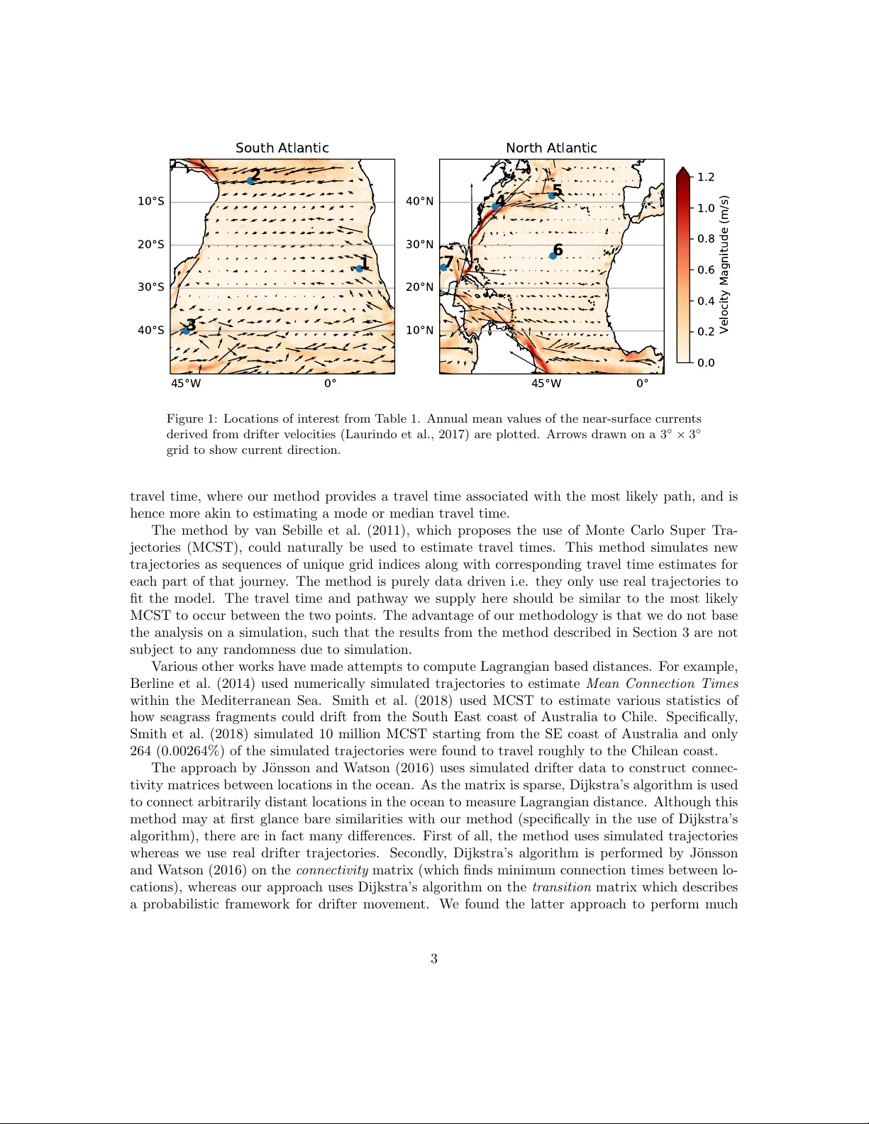
Estimating the tra v el time and the most lik ely path from Lagrangian drifters Mic hael O’Malley 1 , Adam M. Sykulski 1 , Rom uald Laso-Jadart 2 , Mohammed-Amin Madoui 2 Abstract W e pro vide a nov el metho dology for computing the most lik ely path taken b y drifters b et ween arbitrary ﬁxed lo cations in the o cean. W e also provide an estimate of the tra vel time asso ciated with this path. Lagrangian pathw ays and trav el times are of practical v alue not just in understanding surface v elo cities, but also in mo delling the transp ort of ocean-b orne sp ecies suc h as planktonic organisms, and ﬂoating debris suc h as plastics. In particular, the estimated trav el time can be used to compute an estimated Lagrangian distance, which is often more informative than Euclidean distance in understanding connectivity betw een lo cations. Our metho dology is purely data-driven, and requires no simulations of drifter tra jectories, in con trast to existing approac hes. Our metho d scales globally and can simultaneously handle m ultiple lo cations in the ocean. F urthermore, w e provide estimates of the error and uncertain ty asso ciated with both the most likely path and the asso ciated tra vel time. 1 In tro duction The Lagrangian study of transport and mixing in the ocean is of fundamental interest to o cean mo dellers (v an Sebille et al., 2018, 2009; LaCasce, 2008). In particular, the analysis of data obtained from Lagrangian drifting ob jects greatly con tribute to our kno wledge of o cean circulation, e.g. through analysing the accuracy of n umerical and stochastic mo dels (Hun tley et al., 2011; Sykulski et al., 2016), or the use of drifter data to better understand v arious pathw ays and where to search for marine debris (Miron et al., 2019; v an Sebille et al., 2012; McAdam and v an Sebille, 2018). Meehl (1982) used ship drift data to create a surface v elo cit y data set on a 5 ◦ × 5 ◦ grid. These v elo cities w ere used to sim ulate the Lagrangian drift of ﬂoating ob jects in W ak ata and Sugimori (1990). More recen t works focus on using drifting buo ys to deriv e Lagrangian mo dels to discov er areas where ﬂoating debris tends to end up (v an Sebille, 2014; v an Sebille et al., 2012; Maximenk o et al., 2012). Adv ances in technology ha ve resulted in muc h b etter data quality , which no w p ermits the use of more detailed metho dology . The newer mo dels provide densities of where debris ends up on grid scales as small as 0 . 5 ◦ × 0 . 5 ◦ . In this pap er, we prop ose a no vel computationally fast metho d for estimating a so called “most likely p athway” b etw een tw o p oints in the o cean, alongside an estimated trav el time for this path wa y . ∗ 1 STOR-i Cen tre for Do ctoral T raining / Department of Mathematics and Statistics, Lancaster Universit y , UK † 2 G´ enomique M´ etab olique, Genoscope, Institut F. Jacob, CEA, CNRS, Univ Evry , Univ Paris-Sacla y , Evry , F rance 1 The metho d is purely data-driv en. W e demonstrate our methodology on data from the Glob al Drifter Pr o gr am (GDP) , but the metho d is designed to w ork with any Lagrangian tracking data set. Additionally , w e dev elop and test related methodology for pro viding uncertaint y on b oth the path wa ys and the tra vel times. Our method is automated with little expert knowledge needed from the practitioner. W e provide a set of default parameters whic h allo w the metho d to run as in tended. The method simply takes in a set of locations within the o cean, and outputs a data structure con taining most likely paths and corresp onding tra vel time estimates b etw een all pairs of locations. W e focus on a global scale: we aim to pro vide a measure of Lagrangian connectivit y for lo cations whic h are thousands of kilometres apart. An individual drifter tra jectory is unlikely to connect t wo arbitrary lo cations far apart, hence the need for our methodology which fuses information across many drifters. A tool which predicts tra vel times is of practical use in man y ﬁelds. F or example in ecological studies of marine sp ecies, genetic measuremen ts are taken at v arious lo cations in the ocean (W atson, 2018). Euclidean distance is often used as a measure of separability and isolation-by-distance (Bec king et al., 2006; Ellingsen and Gray, 2002) to ﬁnd correlations with diversit y metrics or genetic diﬀeren tiation b etw een communities or p opulations of organisms. Due to v arious currents and land barriers, we exp ect Euclidean distance to often b e a p o or measure of how ‘distan t’ or dissimilar comm unities or p opulations sampled in t wo locations are. The method prop osed in this w ork would use the estimated tra vel times to supply a matrix con taining a L agr angian distanc e measure betw een all pairs of lo cations. This matrix can then be contrasted with a pairwise genetic distance matrix b et ween these lo cations and will yield new insights. In many instances the Lagrangian distance matrix will b e more correlated with genetic relatedness than a Euclidean distance matrix. This observ ation was already made in the Mediterranean Sea when studying plankton (Berline et al., 2014), and oﬀ the coast of California for a sp ecies of sea snail (White et al., 2010). Both of the w orks by Berline et al. (2014) and White et al. (2010) rely on simulating tra jectories from detailed o cean current data sets to estimate the Lagrangian distance. Such approaches do not scale globally and rely on sim ulated tra jectories from currents rather than real observ ations. In Figure 1, w e show seven lo cations plotted on a map with o cean currents. W e use these lo cations as a pro of-of-concept example throughout this pap er. The exact co ordinates are giv en in T able 1. The aim is to introduce and motiv ate a metho d which provides an estimate as to how long it w ould tak e to drift betw een an y tw o of these lo cations. F or example, the tra vel time from lo cation 2 to lo cation 3 in the South Atlan tic Ocean should b e smaller than the return journey due to the Brazil curren t. W e c ho ose to include lo cations in b oth the North and South Atlan tic as w e wish to demonstrate that the metho d successfully ﬁnds pathw a ys linking p oin ts which are extremely far apart. 1.1 Comparison with Related W orks In this section w e giv e a brief ov erview of techniques that hav e used the Global Drifter Program to ac hieve a similar or related task. The work by Rypina et al. (2017) prop oses a statistical approach for obtaining trav el times. A source area is deﬁned such that at least 100 drifters pass through the source area. The metho d fo cuses on obtaining a spatial probability map and a mean trav el time for ev ery 1 ◦ × 1 ◦ bin outside of the source area. This method successfully combines many tra jectories, ho wev er for m ultiple lo cations one w ould hav e to decide on a v arying grid box for each location of in terest. Suc h a grid box m ust b e manually c hosen by the practitioner meaning that the metho d do es not scale w ell with multiple lo cations. Rypina et al. (2017) also focus on estimating a mean 2 45°W 0° 40°S 30°S 20°S 10°S South Atlantic 1 2 3 45°W 0° 10°N 20°N 30°N 40°N North Atlantic 4 5 6 7 0.0 0.2 0.4 0.6 0.8 1.0 1.2 Velocity Magnitude (m/s) Figure 1: Lo cations of in terest from T able 1. Ann ual mean v alues of the near-surface curren ts deriv ed from drifter v elo cities (Laurindo e t al., 2017) are plotted. Arro ws dra wn on a 3 ◦ × 3 ◦ grid to sho w curren t direction. tra v el tim e, where our me th o d pro vides a tra v el time asso ciated with the most lik ely path, and is hence more akin to estimating a mo de or median tra v el time. The me th o d b y v an Sebille et al. (2011), whic h prop oses the use of Mon te Carlo Sup er T ra- jectories (M CST), could naturally b e used to estimate tra v el times. This metho d sim ulates new tra j e ctories as sequences of unique grid indices along with corresp onding tra v el time estimates for eac h part of that jou rney . The metho d is p urely data driv en i.e. they only use real tra jectories to ﬁt the mo del. The tra v el time and path w a y w e supply here should b e similar to the most lik ely MCST to o ccur b et w een the t w o p oin ts. The adv an tage of our m etho dology is that w e do not base the analysis on a sim ulation, s u c h that the results from the metho d describ ed in Section 3 are not sub j e ct to an y randomness due to sim ulation. V arious other w or ks ha v e made attempts to compute Lagrangian based distances. F or example, Berline et al. (2014) used n umerically sim ulated tra jectories to estimate Me an Conne ction Times within the Mediterranean Sea. Smith et al. (2018) used MCST to estimate v arious statistics of ho w se agr as s fragmen ts could drift f rom the South East coast of Australia to Chile. Sp eciﬁcally , Smith et al. (2018) sim ulated 10 mil lion MCST starting from the SE c oast of Australia and only 264 (0.00264%) of the sim ulated tra jectories w ere found to tra v el roughly to the Chilean coast. The approac h b y J¨ onsson and W atson (2016) uses sim ulated drifter data to construct connec- tivit y matrices b et w een lo cations in the o cean. As the matrix is sparse, Dijkstra’s algorit hm is used to connect arbitrarily d is t a n t lo cations in the o ce an to measure Lagrangian distance. Although this metho d ma y at ﬁrst glance bare s imilar ities with our metho d (sp eciﬁcally in the use of Dijkstra’s algorithm), there are in fact man y diﬀerences. First of all, the metho d uses sim ulated tra jectories whereas w e use real drifter tra jectories. Secondly , Dijkstra’s algorithm is p erformed b y J¨ onsson and W atson (2016) on the c onne ctivity matrix (whic h ﬁnds m in im um conn e ction times b et w e en lo- cations), whereas our approac h use s Dijkstra’s algorithm on the tr ansition matrix whic h describ es a probabilistic framew ork for drifter mo v emen t. W e found the latter approac h to p erform m uc h 3 b etter with real data. Finally , we cannot directly implemen t the approac h describ ed in J¨ onsson and W atson (2016) as only connectivity v alues higher than one year are used b y the algorithm. F or real data suc h a step would result in a v ery sparse connectivity matrix making the metho d infeasible. An initial analysis w e conducted using similar methodology ac hieved p o or results. There are a v ariety of w orks which use Mark o v transition matrices for diﬀerent aims to this w ork. Ser-Giacomi et al. (2015b) and Miron et al. (2019) lo ok at probable paths, where b oth of these w orks ﬁnd a path going b etw een t wo p oints in a certain num ber of days using a dynamic program. F royland et al. (2014) and Miron et al. (2017) study o cean dynamics b y analysing eigenv alues of the transition matrix. Other metho ds in the literature include characterizing dispersion and mixing (Ser-Giacomi et al., 2015a), iden tiﬁcation coheren t regions (F royland et al., 2007; Ser-Giacomi et al., 2015a), forward integration of tracers (v an Sebille et al., 2012; Maximenko et al., 2012), and guiding drifter deplo yments (Lumpkin et al., 2016). W e diﬀer from these works as we ultimately aim to ﬁnd trav el times, as w ell as pathw ays, betw een multiple ﬁxed lo cations. Our prop osed algorithm for computing trav el times and pathw ays will also use the aforemen- tioned Marko v transition matrix approach. Our key no velt y is that we build on this conceptual approac h b y implemen ting and demonstrating the b eneﬁts of using the (H3) spatial indexing system for discretization, and by supplying uncertain ty quan tiﬁcation guidelines by applying grid rotations and data b o otstrapping. The steps outlined in Algorithm 1 are individually known across disparate literature, ho wev er, this is the ﬁrst paper to our kno wledge that eﬀectively combines these steps to solv e the problem of interest. W e provide numerous examples to show how our metho dology ro- bustly outperforms state-of-the-art alternativ e approac hes. In addition, we supply freely-a v ailable soft ware in the form of a Python pack age, of which all parameters in the mo del can easily b e customized to suit the needs of the practitioner. In summary , the nov el contributions of this work are: a) the combination of the steps in Section 3 to form a computationally-eﬃcien t algorithm whic h applies directly to transition matrices to ﬁnd most lik ely paths and trav el times sim ultaneously , b) computation of uncertaint y from discretization error and data sampling (Section 4), and c) the demonstration of the metho d sho wing it success- fully obtains robust measures of connectivit y b et ween both v ery distant and closely lo cated p oints (Section 5). The key outcome is that w e obtain o ceanographic tra vel times and most lik ely paths requiring no simulated tra jectories. W e b elieve our method is preferable to Rypina et al. (2017) as w e do not require custom treat- men t to diﬀeren t source areas. J¨ onsson and W atson (2016) requires the simulation of many v ery long and exp ensiv e to compute tra jectories whic h obtain spurious results on real data. Using MCST’s as in Smith et al. (2018) relies on simulation. The estimation of a full pairwise trav el time matrix of the lo cations in T able 1 requires 42 trav el time estimations. With MCSTs this would likely require the simulation of millions of tra jectories and man ual analysis of eac h lo cation pair. Our metho d, in con trast, can pro duce such a trav el time matrix in a matter of seconds given that the transition matrix needs to b e estimated just once a priori . In a similar manner, global tra vel time maps can b e made in a matter of minutes, such as those that w e will b e sho wing in Section 5. 2 Bac kground and Notation 2.1 Global Drifter Program The Global Drifter Program(GDP) is a database managed by the National Oceanographic and A tmospheric Administraction (NOAA) (Lumpkin and Centurioni, 2019; Lumpkin and Pazos, 2007). 4 This data set con tains o v er 20,000 free-ﬂoating buo ys tem p orally spanning from F ebru ary 15, 1979 through to the curren t da y . These buo ys are referred to as drifters . The drifter design comprises of a sub-surface ﬂ oat and a drogue so c k. Often this drogue so c k detac hes. W e refer to the drifters whic h ha v e lost their drogue s o c k as non-drogued drifters, and drogued for those whic h still ha v e the drogue attac hed. Here w e use the drif te r data recorded up to July , 2020. W e use data whic h has b een recorded from drogued drifters only . This results in a total of 23461 drifters b eing used, where the spatial distribution of observ ations is sho wn in Figure 2. Only using drogued drifters is not a restriction, it w ould b e straigh tforw ard to simply use the data from non-drogued drifters if a practitioner w as in terested in a sp ecies or ob ject whic h exp eriences a high wind for c in g, or a com bination of b oth if it is b eliev ed that the s p ecies fol lo w ed a mixture of near surface and wind-for c ed curren ts. The data is qualit y con trolled and in terp olated to six hourly in terv als using the metho dology from Han s en and P oulain (1996). These in terp olated v alues do con tain some noise due to b oth satellite error and in terp olation, ho w ev er, the magnitud e of this noise is negligible in comparison to the size of grid w e use in Section 3. Hence, w e ignore this noise and tr e at the in terp olated v alues as observ ations. F or the same reason w e n ote that the in terp olation metho d used is not imp ortan t here, instead of the six hourly pro duct w e could use the hourly pro duct pro d uce d b y metho dology prop osed b y Elip ot et al. (2016), or drifter data smo othed b y splines as prop osed b y Early and Sykulski (2020). The v alue of using the Glob a l Drifter Program is w e obtain a true mo del-free represen tation of the o cean. All phenomena whic h act on the drifters are accoun ted for in the data set. T h e other common approac h is to ﬁrst obtain an estimate of the underlying v elo cit y ﬁeld, then sim ulate thousands of tra j e ctories using the v elo cit y ﬁeld. While this sim ulation approac h is often satisfactory in some applications, the mo dels ge n e r ally do not agree completely with the actual observ ation s . Spatial distribution of 6 hourly observations 0 1 20 100 500 1000 2000 2494 Count Figure 2: Num b er of observ at ions from the Global Drifter Program in eac h 1 ◦ × 1 ◦ longitude- latitude b o x. 5 2.2 Notation Here we use x ◦ , y ◦ to b e a geographic co ordinate corresp onding to latitude and longitude resp ec- tiv ely . W e refer to the longitude-latitude grid system using the notation x ◦ × y ◦ , which means eac h grid b o x goes x ◦ along the longitude axis and y ◦ along the latitude axis. W e use b old fon t for an y data which is in longitude-latitude pairs; i.e r = r lon , r lat , and non-b old text for either a grid index or a single n umber. W e use S to denote the set of all p ossible grid indices. A full table of notation is given in App endix B. 2.3 Capturing Drifter Motion W e deﬁne the drifter’s probability densit y function as P ( r 1 , t | r 0 , t 0 ) where the drifter started at r 0 ∈ R 2 at time t 0 and mo ved to p osition r 1 ∈ R 2 at time t , where r 0 and r 1 are longitude-latitude pairs. In the absence of a mo del, this probabilit y density cannot b e estimated con tinuously from data alone. Therefore, we follo w previous works whic h spatially discretize the problem (Maximenko et al., 2012; v an Sebille et al., 2011; Miron et al., 2019; Rypina et al., 2017; Lumpkin et al., 2016). Instead of considering r 0 ∈ R 2 , w e consider r 0 ∈ S where S is some set of states which corresp ond to a polygon in space; we will deﬁne how these are formed in Section 3.2. Often these states are simply 1 ◦ × 1 ◦ degree b o xes (e.g. as used in Figure 2). As in Maximenk o et al. (2012), w e assume that the process driving the drifter’s mov emen t is temp orally stationary . That is: P ( r 1 , t | r 0 , t 0 ) = P ( r 1 | r 0 , t − t 0 ) , r 0 , r 1 ∈ S , i.e. the probability of going from r 0 to r 1 dep ends only on the time incremen t. The probability do es not dep end on the start or ﬁnish time. F urthermore, given that w e are using data whic h is observ ed at regular and discrete times, we shall only consider discrete v alues of time. Let s = { s 0 , s 1 , s 2 , . . . , s n } b e a sequence of lo cations equally spaced in time where each entry s i can tak e the v alue of anything within S . W e deﬁne the probabilit y p ( s i +1 = q | s i = k ) as the probability that the position at time i + 1 is q giv en that the state at time i w as k where q, k ∈ S . A Lagrangian decorrelation time causes the drifter to ‘forget’ its history (LaCasce, 2008). W e aim to choose a quantit y which is globally higher than the Lagrangian decorrelation time. The reasoning b ehind using this time is that if w e consider a sequence of observ ations, which are at least the Lagrangian decorrelation time apart then the following Marko v prop ert y is satisﬁed: p ( s i +1 = q i +1 | s i = q i , s i − 1 = q i − 1 , · · · , s 0 = q 0 ) = p ( s i +1 = q i +1 | s i = q i ) , (1) where q i is just some ﬁxed state and s i is the random pro cess. In other words, the Marko v prop erty states that probabilit y of transition to state s i +1 is indep endent of all the past states at times i − 1 and earlier, given the state at time i is kno wn. In this case, the physical time diﬀerence asso ciated with i + 1 and i b eing larger than the chosen Lagrangian decorrelation time v alidates the use of the Mark ov assumption. F or the rest of this pap er we assume that the time b etw een discrete time observ ations is equal to T L . W e call this quantit y the Lagrangian cut oﬀ time. Setting T L higher than the decorrelation 6 time allows us to use the Mark ov prop ert y from Equation (1) freely . In so doing, alongside the simpliﬁcation of discretizing lo cations, this allows the problem to b e treated as a discrete time Mark ov c hain. Here w e ﬁx T L = 5 days as this m atc hes previous similar w orks (Maximenk o et al., 2012; Miron et al., 2019). The estimated decorrelation time for the ma jorit y of the surface of the Ocean is lik ely to b e lo w er than 5 da ys (e.g. see Zh urbas and Oh (2004) for the P aciﬁc and Lumpkin et al. (2002) for regions in the A tlantic). In Appendix E w e conduct a sensitivity analysis to show our results are not o verly sensitiv e to the c hoice of T L as long as T L > 2 da ys. 3 Metho d for Computing the Most Lik ely P ath and T ra v el Time Maximenk o et al. (2012) and v an Sebille et al. (2012) fo cus on the use of a transition matrix estimated from drifters to disco ver p oints where drifters are likely to end up. In this section we build on such an approach by providing a metho d to take suc h a matrix and provide an o cean path wa y and trav el time. In Section 3.1, we explain in detail ho w the transition matrix is formed. As a grid system is needed to form the discretization of data we in tro duce our chosen system in Section 3.2. Then in Section 3.3, w e describ e how we estimate the most likely path of a drifter to hav e taken. Finally , in Section 3.4 w e explain how we turn the most likely path and transition matrix into an estimate of trav el time. W e giv e a summary of ho w this articulates in the pseudo-co de in Algorithm 1. 3.1 T ransition Matrix The lo cation of a drifter at an y given time is a contin uous vector in R 2 , the longitude and latitude of the p oin t. W e deﬁne an injective map which maps this contin uous pro cess onto a discrete set of states which are indexed by in tegers in S . W e deﬁne the map as follows: f : R 2 → S . (2) W e aim to make a Mark ov transition matrix T of size n states ro ws and columns, where T s,q denotes, the probability of movin g from s to q in one time step. Similarly to the approach of Maximenko et al. (2012), we form our transition matrix using a gap metho d. In each drifter tra jectory we only consider observ ations as a pair of points T L da ys apart. When using this metho d for other applications w e advise using T L to be higher than the decorrelation time of velocity to justify the Mark ov assumption. Consider a tra jectory as a sequence of p ositions y j = { y i,j } n j i =1 where j is the j th out of N tra jectories, n j is the num b er of lo cation observ ations in the tra jectory , and y i,j ∈ R 2 are the longitude-latitude p ositions. First, we map eac h tra jectory into observ ed discrete states. W e will denote these states as follo ws, g i,j = f ( y i,j ) . (3) F or each s, p ∈ S we estimate the relev ant entry of our transition matrix T through using the follo wing empirical estimate: T s,p = P N j =1 P n j − 4 T L i =1 I [ g i +4 T L ,j = p ] I ( g i,j = s ) P N j =1 P n j − 4 T L i =1 I [ g i,j = s ] , (4) 7 Where I is the indicator function, suc h that it takes the v alue 1 if the statement inside it is true, and zero otherwise. Note that we take gaps of 4 T L as observ ations are ev ery 6 hours in the GDP application and T L is in days. The estimation of the transition matrix, using the discretization of tra jectories in Equation (3), in com bination with Equation (4), is commonly referred to as Ulam’s approac h (Ulam, 1960). W e exp ect that states in S which are not spatially close will hav e non-zero en tries such that the matrix T will be v ery sparse, but this is not a problem for the metho dology to work o ver large distances as we shall see. 3.2 Spatial Indexing Clearly the resulting transition matrix describ ed in Section 3.1 strongly dep ends on the choice of grid function in Equation (2). Most previous works (v an Sebille et al., 2012; Maximenko et al., 2012; Rypina et al., 2017; McAdam and v an Sebille, 2018; Miron et al., 2019) use longitude-latitude based square grids where all grid b oxes t ypically v ary b et ween 0 . 5 ◦ × 0 . 5 ◦ and 1 ◦ × 1 ◦ . A 1 ◦ × 1 ◦ grid cell around the equatorial region will b e approximately equal area to a 111 . 2km × 111 . 2km square b o x. How ev er, if w e take such a grid ab o ve 60 ◦ latitude, e.g. the Norwegian sea, the grid cell will b e approximately equal area to a 55 . 6km × 111 . 2km square b ox. There are a few other c hoices which we argue are more suitable for tracking moving data on the surface of the Earth. Typically three types of grids exist for tessellating the globe: triangles, squares, or a mixture of hexagons and p en tagons. Here w e choose to use hexagons and p entagons as they ha ve the desirable property that ev ery neighbouring shap e shares precisely t wo v ertices and an edge. This is diﬀeren t to sa y a square grid where only side-by-side neigh b ours share tw o v ertices and an edge, whereas diagonal neigh b ours share only a vertex. This equiv alence of neighbors property for hexagons and p entagons is clearly desirable for the tracking of ob jects as this will result in a smo other transition matrix. W e sp eciﬁcally use the grid system called H3 b y UBER (UBER, 2019). This system divides the glob e such that an y longitude and latitude coordinate is mapp ed to a unique hexagon or p entagon. This shap e will ha v e a unique ge ohash which w e can use to k eep track of grid index. The b eneﬁt of using such a spatial indexing system is that attention is paid to ensuring that each hexagon is appro ximately equal area. W e use the r esolution 3 index where each hexagon has an a verage area of 12 , 392km 2 . A square b ox of size 111 . 32km × 111 . 32km has roughly the same area as this which is v ery similar to the size of a 1 ◦ × 1 ◦ grid cell near the equator. An example of an area tessellated b y H3 is sho wn in Figure 3. Other potential systems which could b e used include S2 by Go ogle whic h is a square system, or simply using a longitude-latitude system as v arious other w orks do. W e show some example path w ays using diﬀeren t grid systems and resolutions in the Supplemen tary Information Figure S1. The longitude-latitude system results in pathw ays that unrealistically follow long blo c k-wise vertical or horizon tal straight line motions, in cont rast to the more realistic and meandering pathw a ys pro duced b y the hexagonal-p entagonal H3 grid system. 3.3 Most Likely P ath F or our analysis, the ﬁrst step is to deﬁne a most lik ely path. A path is simply a sequence of states suc h that the ﬁrst elemen t is the origin and the last element is the destination. W e also require that tw o neighboring states are not equal to each other. Deﬁnition 1 (P ath) . We deﬁne the sp ac e of p ossible p aths P o,d , b etwe en the origin o ∈ S and 8 Figure 3: A small area around the Strait of Gibraltar whic h is tessellated using the H3 spatial index. W e sho w resoluti ons 1, 2 and 3 in red, blue and blac k resp ectiv ely . Blac k is the resolution used in this w ork. destination d ∈ S , as the fol lowing: P o,d = { p = ( p 0 , p 1 , p 2 , . . . , p n ) : p i ∈ S ∀ i ∈ { 1 , . . . , n − 1 } , p 0 = o, p n = d, p i − 1 6 = p i } . With a c ar dinality op er ator | p | = n which denotes the length of the p ath. Giv en the transition matrix T w e deﬁne the probabilit y of suc h a path: P ( p ) = n − 1 Y i =0 P ( s i +1 = p i +1 | s i = p i ) = n − 1 Y i =0 T p i ,p i +1 . (5) Deﬁnition 2 (Most lik ely path) . Consider any p ath p ∈ P o,d = { p 0 , p 1 , p 2 , . . . , p n } . By the most likely p ath ˆ p we me an the p ath which maximises the pr ob ability of observing that p ath. ˆ p = arg max p ∈P o,d { P ( p ) } = arg max p ∈P o,d ( n − 1 Y i =0 T p i ,p i +1 ) . (6) Optimising Equation (6) app ears in tractable at ﬁrst glance. Ho w ev er, this c an easily b e solv ed with shortest path algorithms suc h as Dijkstra’s algorithm (Dijkstra, 1959). W e giv e pr e cise details on ho w to ﬁnd this path w a y in App endix C. 3.4 Obtaining a tra v el time es tima te The most lik ely path is often a quan tit y of in terest in itself, h o w ev er w e can also obtain a tra v el time estimate of this path. The metho d should b e fast and eﬃcien t as it should b e able to run 9 for large sets of lo cations quickly . W e ac hiev e this by giving a formula to estimate the tra vel time based directly on the transition matrix. Consider the path, p = { p 1 , . . . , p n } , from whic h w e aim to estimate the exp ected tra v el time. The key consideration this section addresses is: the path is a sequence of unique states, whereas when sim ulating from a discrete time Mark ov c hain, the chain has a probabilit y of remaining within the same state for m ultiple time steps. W e therefore aim to obtain an estimate of ho w long the Mark ov c hain takes, on a verage, to jump b et ween p i and p i +1 , and then aggregate this ov er the path to form a tra vel time estimate. W e assume that the only p ossibilit y is that the drifter follows the path we are interested in. So p i m ust b e follow ed by p i +1 . Now w e use t to index the time of the Marko v chain and suppose s t = p i . W e are then interested in the random v ariable k where t + k is the ﬁrst time that the pro cess transitions from p i to p i +1 . Note that the only p ossibilit y for states { s t + l } k − 1 l =1 is that they are all p i , otherwise the ob ject w ould not b e following the path of in terest. Therefore, we obtain the distribution of k as follo ws (pro of in Appendix D.1): P ( s t + k = p i +1 , { s t + l = p i } k − 1 l =1 | s t = p i , p } ) = T p i ,p i +1 T k − 1 p i ,p i ( T p i ,p i + T p i ,p i +1 ) k . (7) Note that if w e set a = T p i ,p i T p i ,p i + T p i ,p i +1 in Equation (7) w e get: P ( s t + k = p i +1 | s t = p i , p ) = a k − 1 (1 − a ) , (8) whic h is the probability distribution function of a negativ e binomial distribution with success prob- abilit y a and num ber of failures b eing one. W e denote the random v ariable for the tra vel time b et ween p i and p i +1 as k i . As the negativ e binomial distribution corresp onds to the time un til a failure, w e are in terested in taking one time increment longer than this as we require k i to be the time that we mov e from p i to p i +1 i.e. the time of the failure. Therefore the distribution of k i exactly follo ws k i − 1 ∼ NB(1 , a ). Also, note that k i is in units of the chosen Lagrangian cutoﬀ time T L . T o get the expectation of the total Lagrangian tra vel time w e consider the sum of all the individual parts of the tra vel times k = P n − 1 i =0 k i , such that w e obtain: E [ k ] = n − 1 X i =0 E [ k i ] = n − 1 X i =0  T p i ,p i T p i ,p i +1 + 1  , (9) where we ha ve used that the exp ectation of the negativ e binomial is E [ x ∼ NB(1 , a )] = a 1 − a . W e could attempt to obtain a simple v ariance estimate for the estimate E [ k ] with classical statistics. Ho w ever, w e would only b e able to account for v ariabilit y within the estimates of the en tries T , as w e would hav e to assume p is kno wn. In our case we are interested in the time of ˆ p , which is itself an estimate as it dep ends on T . Obtaining any analytical uncertaint y in the estimation of the most likely path would b e intractable due to the complexity of the shortest path algorithm. Therefore, we prop ose to address the issue of uncertaint y in E [ k ] and p due to data randomness in Section 4.2 using the non-parametric b o otstrap. T o ﬁnish this section, we provide the pseudo-co de for our approac h in Algorithm 1. 10 Input: Drifter data set y , a set of lo cations x , Lagrangian cutoﬀ time T L Map all the drifter locations y to their grids g j,i = f ( y j,i ) using the map from Equation (2). Map all the locations of in terest to their grids g x i = f ( x i ). F orm transition matrix T using Equation (4). for e ach unique p air o and d in { g x i } x i ∈ x do Find and store the most likely path ˆ p o,d b y optimizing Equation (6). Using this path, ﬁnd and store the exp ected trav el time E [ ˆ k o,d ] using Equation (9). end Result: T rav el times E [ ˆ k o,d ] for every pair of lo cations in x and a corresp onding path ˆ p o,d giv en as a sequence of grid indices in S . Algorithm 1: Pseudo-code which summarises how Section 3 is used to turn drifter data and a spatial index function in to most likely paths and trav el time estimates. 4 Stabilit y and Uncertain t y 4.1 Random Rotation A k ey consideration is that the ﬁnal results of the algorithmic approac h may strongly rely on the precise grid system f chosen in Equation (2). T o address the uncertain t y due to the discretization w e prop ose to r andomly sample a new grid system then run the algorithm for the new grid system. In a simple 2d square grid one could simply sample a new grid system by sampling tw o num bers b et ween 0 and the length of a side of the square, then shifting the square by these sampled amoun ts in the x and y direction. In global complicated grid systems such as the one we consider here prop osing uniform random shifting is not trivial. Rather than trying to reconﬁgure the grid system, instead we suggest a more universal alterna- tiv e. W e suggest randomly rotating the longitude-latitude locations of all the relev ant data using random rotations. Such a strategy will w ork for any spatial grid system as it just inv olves a pre- p ossessing step of transforming all longitude-latitude co ordinates 1 . Note that for each rotation w e are required to re-assign the p oints to the grid and re-estimate the transition matrix. These are the tw o most computationally exp ensiv e pro cedures of the metho d. T o generate the random rotations we use the method suggested b y Sho emake (1992). In summary , it amoun ts to generating 4 random num b ers on a unit 4 dimensional hypersphere as the quaternion representation of the 3 dimensional rotation, which can equiv alently b e represented as a rotation matrix M . Then w e apply this rotation to the Cartesian representation of longitude and latitude. T o obtain trav el times which remo ve bias eﬀects from discretization, we sample n rot rotation matrices M ( i ) . W e then run Algorithm 1, how ev er as a prep ossessing step we rotate all locations of the drifter tra jectories and lo cations of interest. F or eac h rotation matrix this will result in a set of trav el times ˆ d ( i ) . The sample mean of these rotations will b e more stable than the v anilla metho d. The sample standard deviation will inform us ab out uncertaint y in trav el times due to discretization. 1 Conditional on the grid system having a reasonable minimum area. This metho d rotates the p oles to a random point, whic h w ould giv e spurious results in a longitude-latitude grid. Thus providing another reason why the H3 system is more suitable. 11 4.2 Bo otstrap If w e required a rough estimate of uncertaint y we could consider that ˆ p , the most lik ely path, is ﬁxed and then estimate V ar[ ˆ k ]. How ev er, this w ould be a p oor estimate because such an estimate would assume that: (1) the transition matrix entries follo w a certain distribution, and (2) the path ˆ p is the true most likely path. In realit y neither of these are true, they will b oth just b e estimates. The transition matrix elemen ts are estimated from limited data and the shortest path strongly dep ends on the estimated transition matrix, e.g. a small change in the transition matrix could result in a signiﬁcan tly diﬀerent path. Therefore, we obtain estimates of uncertaint y by b ootstrapping (Efron, 1993). Bo otstrapping is a method to automate v arious inferential calculations by resampling. Here the main goal is to estimate uncertaint y around ˆ θ = E [ ˆ k ]. The b o otstrap inv olves ﬁrst resampling from the original drifters to obtain a new data set. W e call y ∗ = { y ∗ j } j =1 ,...N a b o otstrap sample, where y ∗ j is a drifter tra jectory whic h has been sampled with replacement from the original N drifters. Then we use y ∗ as the input dataset to Algorithm 1. W e do this resampling B times to obtain B estimates of ˆ θ = E [ ˆ k ], we denote these b o otstrap estimates as { ˆ θ ( b ) } B b =1 . W e then estimate our ﬁnal b o otstrapp ed mean and standard deviation estimates as the follo wing: sd 2 boot =    P B b =1  ˆ θ ( b ) − ˆ θ ( . )  2 B − 1    , where ˆ θ ( . ) = B X b =1 ˆ θ ( b ) /B . (10) In addition to the uncertaint y measure in trav el time that b oth the b o otstrap and rotation metho dology provide, these metho ds also supply a collection of sample most lik ely paths. These paths can be used to in vestigate v arious phenomena, such as why the uncertaint y is high. W e can plot the paths for a ﬁxed origin-destination pair and ma y see for example that many paths follow one curren t where another collection of paths follo w a diﬀerent current. W e giv e n umerous examples of this in Sections 5.2 and 5.3. 5 Application W e use the lo cations giv en in T able 1 for the demonstration of the method describ ed in this paper. These locations were chosen for multiple reasons; (1) they were placed on or near o cean curren ts, suc h as the South A tlantic current, the Equatorial current and the Gulf Stream; the magnitudes of whic h can b e seen in Figure 1, and (2) stations w ere placed in b oth the North and South A tlan tic to show ho w the method can ﬁnd pathw a ys whic h are not trivially connected. First we go ov er an application of the v anilla metho d from Section 3, then w e provide brief results using the adaptations using b ootstrap and rotations from Section 4 in Section 5.2 and Section 5.3 resp ectively . W e supply a link to a Python pack age and co de used to create these results in the App endix. Prior to our analysis we take a practical step to improv e the reliability of the metho d. we ﬁnd the states corresp onding to − 79 . 7 ◦ , 9 . 07 ◦ , − 80 . 73 ◦ , 8 . 66 ◦ (t wo p oints on the Panama land mass), − 5 . 6 ◦ , 36 ◦ and − 5 . 61 ◦ , 35 . 88 ◦ (t wo p oints on the Strait of Gibraltar), then remov e the 12 Longitude Latitude 1 9.0 -25.5 2 -25.0 -5.0 3 -45.0 -40.0 4 -69.0 39.0 5 -42.5 41.5 6 -42.0 27.5 7 -93.2 24.8 T able 1: T able of station locations corresp onding ro ws and columns from T . If this step is not taken the metho d often uses pathw ays crossing the P anama land mass, resulting in imp ossibly short connections to the P aciﬁc Ocean. The reasoning for remo ving the p oints on the Strait of Gibraltar is data-driven, further details are in the supplemen tary information, particularly ho w one can adapt the metho d to sp ecify trav el times in to and out of the Mediterranean sea. Figure 4 shows the pathw a ys b et ween a represen tative sample of the stations. First we note what features are observed in the most likely path. The Gulf Stream is used on almost ev ery path trying to access locations 4, 5 or 6 in Figure 4. Observe in Figure 4 c ) when going from lo cation 3 to 5 that the metho d chooses to en ter the Gulf of Mexico and then uses the Gulf Stream to access lo cation 5, even though the actual geo desic distance of this path is long. Other examples whic h use the Gulf Stream include d ) and h ). Generally , an y of the paths leaving lo cation 1 and attempting to trav el northw est use the Benguela Curren t, for example Figure 4 a ), i ) and g ). The trav el times obtained b etw een the sample stations in Figure 4 show interesting results regarding the lack of symmetry when reversing the direction of the path b et ween tw o stations. When going from location 2 to lo cation 4 w e estimate a long most lik ely path in terms of physical distance. How ev er, the resulting trav el time of this path (0.7 y ears) is smaller than the trav el time of the more direct path from lo cation 4 to lo cation 2 (4.8 years) - which is m uch shorter in distance. This is b ecause the path going from lo cation 2 to lo cation 4 follows strong currents suc h as the North Equatorial current and the Gulf Stream. Another interesting result is that going from 3 to 5 and vice versa are relativ ely close in terms of trav el time even though 3 to 5 uses the Gulf Stream but the return does not. In the most likely path from 3 to 5, up until around − 16 ◦ latitude the tra vel time is 5.2 years, whic h w e exp ect as the path wa y seems to b e going against the Brazil curren t. After this p oin t the rest of the path takes the remaining 3 y ears despite the remainder b eing ov er half the actual ph ysical distance of the path wa y . W e expect this short time is due to the metho d ﬁnding a pathw ay along the North Brazil curren t, follo wed by the Caribbean curren t, follo wed b y the Gulf Stream. 5.1 Global T ra vel Times Figure 5 shows the trav el time distribution to and from tw o ﬁxed lo cations, taken to matc h the studied lo cations of J¨ onsson and W atson (2016), to the en tire glob e. W e note that the trav el time map is less smo oth than the one shown in J¨ onsson and W atson (2016). The black and purple areas how ever (up to 5 y ears tra vel time) are similar to those found in J¨ onsson and W atson (2016), sho wing agreement ov er short spatial scales. When it comes to larger distances we generally ﬁnd 13 a) 1 -> 2: 2.1 Years 2 -> 1 : 3.2 Years 1 2 3 b) 1 -> 3: 4.6 Years 3 -> 1 : 2.7 Years 1 2 3 c) 3 -> 5: 8.2 Years 5 -> 3 : 7.6 Years 1 2 3 4 5 6 7 d) 6 -> 7: 2.7 Years 7 -> 6 : 3.2 Years 2 4 5 6 7 e) 4 -> 6: 3.3 Years 6 -> 4 : 5.6 Years 2 4 5 6 7 f) 3 -> 6: 7.6 Years 6 -> 3 : 5.3 Years 1 2 3 4 5 6 7 g) 1 -> 7: 3.3 Years 7 -> 1 : 8.8 Years 1 2 3 4 5 6 7 h) 2 -> 4: 0.7 Years 4 -> 2 : 4.8 Years 1 2 3 4 5 6 7 i) 1 -> 6: 4.2 Years 6 -> 1 : 10.8 Years 1 2 3 4 5 6 7 Figure 4: Ex a mple path w a ys found from the metho d. Sequences of blue hexagons are going from the lo w er n um b er to the higher n um b er. Sequences of red hexagons are going from the higher n um b er to the lo w er n um b er. Num b ered lo c ations are as in T able 1. The exp ected tra v el time of the most lik e ly path is giv en in the title of eac h plo t. Similar plots can b e pro vided for ev ery lo cation pair using the onlin e co de, ho w ev er these are not presen ted here o wing to p age length c onsiderations. the maps are mark edly diﬀeren t. F or example the y ello w patc h in the north east paciﬁc in Figure 5c is not seen in J¨ onsson and W atson (2016). Su c h discrepancies can b e attributed to man y reasons 14 a) Travel times to star from the rest of the globe b) Travel times from star to the rest of the globe c) Travel times to star from the rest of the globe d) Travel times from star to the rest of the globe 0 5 10 15 20 25 30 Travel Time (Years) Figure 5: T ra v el times of the most lik ely path orig inating from the red stars and going to or from (indicated b y the title) the cen troid of a 2 . 5 ◦ × 2 . 5 ◦ square grid system. Figure setup and lo cations tak en to matc h Figure 2 of J¨ onsson and W atson (2016). suc h as: (1) they reﬂect the diﬀerence in metho ds, where w e use a transition matrix approac h, and J¨ onsson and W atson (2016) use a connectivit y matrix; (2) J¨ onss on and W atson (2016) aim to ﬁnd the shortest path in time, whereas w e aim to ﬁnd the exp ected time of the most lik ely path; and (3) the results sho wn here are deriv ed from real data, whereas J¨ onsson and W atson (2016) use sim ulated tra jectories. W e sho w an example in Figure 6 whic h explains the lac k of spatial smo othness in Figure 5, where w e sho w t w o path w a ys b oth originating from a ﬁxed p oin t and ending at t w o distinct p oin ts only 1 ◦ latitude apart. The p oin ts are on either side of the discon tin uit y in th e north-east P aciﬁc seen in Figure 5c. The path w a ys b ecome visibly diﬀeren t af te r they ha v e b oth reac hed the south P aciﬁc. Suc h a phenomenon results in the lac k of spatial smo othness of tra v el time distribution s . This demonstrates that the tra v el times do not necessarily ob ey the triangle inequalit y . If smo othn e ss 15 is desired w e sho w an alternativ e approac h in the supplemen tary information, where instead a minim um tra v el time is the ob jectiv e, whic h is then more analogous to the J¨ onsson and W atson (2016) approac h. W e argue ho w ev er that the exp ected tra v el time of the most lik e ly path, rather than the minim um tra v el time, is a more relev an t metric for estimating connectivit y and Lagrangian distance in application s measuring spatial d e p endence b et w een p oin ts in the o cean. Path from SE africa to ( 1 3 2 , 2 5 ) b l u e , ( 1 3 1 , 2 5 ) g r e e n . Figure 6: The most lik ely path from t w o p oin ts in the North P aciﬁc to th e south-east coast of Africa. The green and blue path w a ys are almost iden tical as they cross the south A tlan tic. The path w a ys diﬀer greatly ho w ev er as they cross the P aciﬁc, ev en though the t w o starting p o in ts in the north P aciﬁc are only 1 degree apart. The path going from − 131 ◦ , 25 ◦ has an exp e cted tra v el time of 21.2 y ears, the path going from − 132 ◦ , 25 ◦ has an exp ected tra v el time of 11.4 y ears. 5.2 Bo otstrap T o sho w the v alue of the b o otstrap w e sho w the results for one particular pair of stations, the path w a y going from lo cation 1 to lo cation 3 and bac k. The path w a ys whic h result from the b o otstrap are sho wn in the b ottom panel of Figure 7. The dark er lines on the ﬁgu re imply that that this transition is used more of te n . W e see that f or most of the journey the dark er lines closely follo w the original path. The b o otstrap disco v e r s some sligh tly diﬀeren t paths, for example around − 20 ◦ Longitude the path going from 3 to 1 o ccasionally seems to ﬁnd that going furt he r south is a more lik ely path. Also, around the b eginning of the path going from 1 to 3, w e see that the most lik ely path tak en most frequen tly b y the b o otstrap samples often do es not follo w the most lik ely path from the full data. The main goal of the b o otstrap is that w e obtain an estimate of the s tan dard errors. In this case w e get standard error estimates using Equation (10) of 0.5 y ears for going from 3 to 1 and 0.6 y ears for going from 1 to 3. In general, w e found that the standard error w as lo w er when the path follo ws the d irec ti on of ﬂo w. The top ro w of plots in Figu re 7 app e ar s to sho w that there is a sligh t bias b et w een the b o otstrap mean and the v anilla metho d tra v el time. W e b eliev e this is due to the v ariance within the paths. The mean estimated from the b o o t s trap samples are c lose to the estimates from the rotati on metho d w e will shortly presen t in Figure 9. T h e rotation mean estimates ar e within 0.4 y ears of the b o otstrap me ans in b oth cases sho wn here. 16 2 4 6 Travel Time (Years) 0 20 Count Bootstrap Times: 3 - > 1 2 4 6 Travel Time (Years) 0 20 40 Count Bootstrap Times: 1 - > 3 40°W 20°W 0° 40°S 40°S 30°S 30°S 20°S 20°S 1 3 Figure 7: Tw o b o otstrap distributions of tra v el times are sho wn in the top ro w resulting from 200 b o o tstrap samples. The v ertical line is the tra v el tim e if th e full data is used to estimate the path and time. T he corresp onding b o o tstrapp ed paths are sho wn in the b ottom ﬁgure. Blue lines and hexagons are for going from 1 to 3, re d lines and hexagons are for going from 3 to 1. The l ines connect the cen troi ds of the spatial index of the b o otstrapp ed paths. Dark er lines mean that path is tak en more often. The ligh t hexagons are the path w a y tak en if the full data i s used with no resampling i.e. the path w a y sho w n in Figure 4. 5.3 Rotation If w e consider t w o p oin ts in the same H3 Index, for example lo cation 1 (9 ◦ , − 25 . 5 ◦ ) and a new p oin t 9 ◦ , − 26 . 2 ◦ (as sho wn in Figure 8), then using the original grid system the metho d will simply pro duce a tra v el time of 0. T o solv e this problem, w e consider using 100 rotations as explained in Section 4.1. F or eac h rotation w e estimate the tra v el time b oth bac k and forth. In 22 of the rotations the t w o p oin ts ended up in the same hexagon, hence resulting in a zero tra v el time . W e plot the distribution of th e other 78 tra v el times in the b ottom ro w of Figure 8. The mean of all the en tries including the ze r os is 20.5 da y s for going from the new p oin t to lo cation 1, and 22.2 da ys for going from lo cation 1 to the new p oin t. The second b eneﬁt of p erforming rotations is to mak e estimates less dep enden t on the grid system. W e use t he same 100 rotations as with the previous example, and compute the most lik ely path and the mean tra v el times. In Figure 9 w e plot the path w a ys with the mean and standard deviation of the tra v el tim es resulting from these 100 rotations. The tra v el ti m es and paths sho wn in this ﬁ gure are comparable to those giv en in Figure 4. In most of the path w a ys w e see that the dark est, most p opular paths matc h up with the path w a ys in Figure 4. One of the more in teresting results from this analysis is the path going from 2 to 1 in Figure 9 a). Most of the paths go u p closer to the Equator, then use the Equatorial Coun ter curren t, f ollo w ed b y the Guinea and Gulf of Guinea curren ts as in the original v anill a application of the metho dology . A small n um b er of the rotations res u lt in p ath w a ys that end up crossing the South A tlan tic, to th e south of lo cation 2, then follo ws the South A tlan tic curren t o v er to lo c ati on 1. In general, the tra v el times from the rotation and original metho d can b e signiﬁcan tly diﬀeren t, whic h supp orts the need for this rotation metho dology . If w e c ompare Figure 4 and Figure 9, most of the distances sta y close to what they w ere in the origin al results using no rotations. W e see that going from 6 to 4 drops from 5. 6 y ears in Figure 4e) to 3.8 y ears in Figure 9e) and 4 to 6 increases from 3.3 y ears to 5.4 y ears. This causes the ordering of the distances to c hange as 6 to 4 is no w the shorter t ra v el time. W e b eliev e the cas e in e) is mainly due to 4 b eing lo cated just north w est 17 7°E 8°E 9°E 10°E 11°E 27°S 27°S 26°S 26°S 25°S 25°S 0 20 40 Travel time (days) 0 10 20 30 Count red -> blue 0 20 40 Travel time (days) 0 10 20 blue -> red Figure 8: Plot of lo cat ion 1 from T able 1 and the p oin t 9 ◦ , − 26 . 2 ◦ , whic h is 0 . 7 ◦ south of lo c ation 1. The relev an t H3 hexagon is plotted o v er the p oin ts. In the b ottom ro w w e plot the histogram and densit y estimate of the tra v el times in eac h direction from applying 100 rotations. The 22 zeros for when the t w o lo cations are in the same hexagon are not included in the histogram. of the stronger curren ts of th e Gulf Stream, whic h mak es it sensitiv e to the grid sys tem. Ho w ev er, the high standar d errors in Figure 9 suggest w e are uncertain ab out this tra v el time. 6 Discussion and Conclusion In con trast to v an Sebille (2014), our m etho dology as presen ted do e s not tak e in to accoun t season- alit y . W e ha v e a few ideas for ho w seasonalit y could b e incorp orated in fu ture w or k. An ob vious adaptation, if the aim w as to obtain a short tra v el time whic h is exp ected to lie in a small 3 mon th windo w, is to just estimate T using drifter observ ations whic h are in that time windo w. Alter- nativ ely , w e could use T L to b e a certain jump suc h as a gap of t w o mon ths, then w e estimate 6 transition matrices sa y T ( k ) , where the en tries T ( k ) i,j are probabilities of going from th e previous time p erio d at state i to state j at the curren t time. Suc h a set up could still b e solv ed using our shortest path algorithm. W e justify our approac h in the same w a y as Maximenk o et al. (2012): w e aim to pro v ide a global view and a s i m p le general concept explainin g the pattern of p oten tial path w a ys and tra v el times. The base metho d can then b e adapted b y practition e rs to accoun t for lo cal spatial or temp oral considerations. More results demonstrating the robustness of our metho d, and motiv ation of parameter c hoices, can b e found in the supplemen tary information. A k ey ﬁnding w e di s cuss here, is that w e found the siz e of the grid system aﬀects the estimated tra v el times signiﬁcan tly , regardless of whether the lat-lon or the H3 grid system is used. Therefore w e do not recommend comparing tra v el times obtained from t w o diﬀeren t grid sizes. Generally the results ar e correlated in an order compari s on sense, ho w ev er, their magnitudes c hange. T ypically a smaller grid sys t e m results in shorter tra v el 18 a) 1 -> 2: 2.2(sd 0.3) Years 2 -> 1 : 3.9(sd 1.1) Years 1 2 3 b) 1 -> 3: 4.1(sd 0.6) Years 3 -> 1 : 2.3(sd 0.5) Years 1 2 3 c) 3 -> 5: 6.9(sd 2.5) Years 5 -> 3 : 7.9(sd 1.5) Years 1 2 3 4 5 6 7 d) 6 -> 7: 2.7(sd 0.3) Years 7 -> 6 : 2.7(sd 0.7) Years 2 4 5 6 7 e) 4 -> 6: 5.4(sd 3.5) Years 6 -> 4 : 3.8(sd 1.6) Years 2 4 5 6 7 f) 3 -> 6: 7.4(sd 2.4) Years 6 -> 3 : 5.8(sd 1.0) Years 1 2 3 4 5 6 7 g) 1 -> 7: 3.2(sd 0.4) Years 7 -> 1 : 10.7(sd 2.8) Years 1 2 3 4 5 6 7 h) 2 -> 4: 0.8(sd 0.1) Years 4 -> 2 : 7.6(sd 2.6) Years 1 2 3 4 5 6 7 i) 1 -> 6: 4.3(sd 0.4) Years 6 -> 1 : 7.7(sd 1.7) Years 1 2 3 4 5 6 7 Figure 9: This ﬁgure l a y out is the same a s in Figure 4, ex c ept here w e plot paths resulting from 100 random rotations. Eac h line connects the ce n troid of eac h hexagon within the path. Note that the hexagons no w come from rotated grid systems, so the cen troids could b e at an y lo c ation hence the smo oth con tin uous lo oking line s. The lines are plotted w ith transparency , when m ultiple lines o v erlap these lines will lo ok dark er. Standard deviations of the tra v el times of the 100 paths are rep orted in the title of eac h ﬁgure. times. Due to this w e w ould only advise the results to b e used in relativ e comparison to eac h other, for example b y sa ying that the tra v el time from a to b is t wice that than from b to c , where b oth 19 times are obtained with the same grid system. The c hoice to show resolution 3 in this pap er w as found to p erform robustly (balancing the error from discretisation and data sparsit y), and follows grid sizes that approximately match previous w orks where 1 ◦ × 1 ◦ grids are used, but this can b e c hanged easily in the online pack age. The use of the b ootstrap and rotations are relatively easy methods to implement, each of whic h pro vides eﬀective estim ates of uncertaint y from data uncertain ty and discretisation resp ectiv ely . Ho wev er, com bining these pro cedures in to one requires careful consideration. If we wan ted to run n rot rotations and B b ootstraps for each rotation, w e still require a metho d to combine these estimates of trav el times. W e could treat every rotation equiv alen tly , so say that our b o otstrap sample in Equation (10) is all n rot × B samples to obtain an estimate of uncertaint y in tra vel time due to the combination of grid discretization and data randomness. Additionally , w e could decomp ose the uncertaint y and pro vide a standard error for just the data randomness by estimating a standard error for each rotation using just the B samples in eac h rotation, and then taking the a verage of all n rot standard error estimates. Our choice of the Lagrangian decorrelation time of 5 da ys ma y be to o low in some instances. Previous works hav e found correlations in the v elo city data lasting longer than 5 da ys in certain regions (Lumpkin et al., 2002; Zh urbas and Oh, 2004; Elip ot et al., 2010). This may suggest that using a larger v alue for T L ma y b e needed to justify the Mark ov assumption. The tradeoﬀ ho wev er is resolution, where shorter timescales allow pathw ays and distances to b e computed with more detail. Our metho dology is designed ﬂexibly such that the practitioner can pic k the most appropriate timescale for the spatial region and application of in terest. In general some unexp ected features of the metho d do occur suc h as the discontin uity discussed in Section 5.1. W e exp ect there would b e less of a discontin uit y if these times were computed with the rotation metho dology , how ever w e argue that the discon tinuities with trav el times of most lik ely pathw a ys should alw ays exist. If smo othness of tra vel times was a ma jor requiremen t, then one could consider the shortest path in tra vel time rather than the most likely path. W e brieﬂy sho w this adaptation in the supplemen tary information. W e exp ect the results w ould require more careful c hecking in such an approach, as the shortest path would b e more likely to use an y glitches in the grid system suc h as if there was a connection o ver P anama. T o summarize, in this paper w e hav e created a nov el metho d to estimate Lagrangian path w ays and trav el times b etw een o ceanic locations, th us oﬀering a new, fast and intuitiv e tool to improv e our knowledge of the dynamics of marine organisms and o ceanic transp ort and global circulation. Ac kno wledgments The w ork of M. O’Malley w as funded b y the Engineering and Ph ysical Sciences Res earc h Council (Gran t EP/L015692/1). The w ork of A. M. Sykulski was funded by the Engineering and Physical Sciences Research Council (Gran t EP/R01860X/1). Data Av ailability Statemen t The drifter data w ere provided by the Global Drifter Program (Lumpkin and Cen turioni, 2019). The curren ts used for visualisation purp oses in Figure 1 are V3.05 of the dataset supplied on the Global Drifter Program w ebsite (Laurindo et al., 2017). 20 A P ac k age Co de to repro duce all ﬁgures related to the method is av ailable at https://github.com/MikeOMa/ MLTravelTimesFigures whic h dep ends on the p ython pack age implementing all of the abov e meth- o ds in this pap er at https://github.com/MikeOMa/DriftMLP . The pac k age takes roughly 3 min- utes total to go from raw data to a pairwise tra vel time matrix for the locations sho wn in T able 1 using Algorithm 1. B T able of Notation W e include a table of mathematical notation for reader reference in T able 2. C Finding the shortest path T o solv e the optimization of Equation (6), we can equiv alen tly consider the log of P ( p ): log P ( p ) = n − 1 X i =0 log T p i ,p i +1 . Then we use the fact that: ˆ p = arg max p ∈P o,d { log P ( p ) } = arg min p ∈P o,d {− log P ( p } ) = arg min p ∈P o,d ( − n − 1 X i =0 log T p i ,p i +1 ) . (11) No w in this form this can be solved using the v ast literature on shortest path algorithms. D Shortest P ath Algorithms Shortest path algorithms (Gallo and Pallottino, 1988; Dijkstra, 1959), such as Dijksta’s algorithm, are p opular algorithms which ﬁnd the so called s hortest path within a graph. In our case the graph is formed such that the vertices or no des uniquely corresp ond to a grid system index, i.e. a ro w/column in the transition matrix T . If there is a non-zero probabilit y in T i,j w e add an edge denoted e i,j , where the w eight on this edge is denoted w ( e i,j ) = − log( T i,j ) b et ween the vertex i and going to the vertex j . Note that T i,j is not necessarily the same as T j,i , hence we hav e a dir e cte d gr aph . Giv en a start v ertex o and an end vertex d , shortest path algorithms will ﬁnd the path P = { v 1 . . . , v n } such that P minimises the follo wing n − 1 X i =1 w ( e v i ,v i +1 ) , hence it solv es the problem in Equation (11). The algorithm used is exact, hence if no path is found then no path exists giv en the curren t netw ork. 21 P ( x | y ) denotes the probabilities of ev ent(s) x given that y occurs. E [ x ] The exp ectation of x . f ( s ) The discretization function i.e. H3. I ( x ) Indicator function giving 1 if x is true and 0 otherwise. arg max x ∈ S An op erator which gives the input v alue, whic h maximises the function q , restricted to the set S . T , T i,j T denotes transition matrix, with en tries T i,j . i, j ∈ S , de- noting the probabilit y of mov- ing from state i to j in T L da ys. x ◦ × y ◦ refers to a longitude-latitude grid system, x degrees in the longitudinal direction, y de- grees in the latitudinal direc- tion. T L Lagrangian cut oﬀ time. S The set of all possible spatial indices. P o,d The set of all p ossible paths going from o to d . p = { p i } n i =1 A path wa y of length n . Indicates a sequence p 1 , p 2 , . . . , p n . All p i ∈ S . k The exp ected tra vel time of a path p . ˆ p , ˆ k Hat notation implies w e are considering the most likely path and trav el time of that path resp ectiv ely . s t used to index the state of the Mark ov c hain after t steps. T able 2: T able of mathematical notation. 22 D.1 Deriv ation of Equation 7 The deriv ation uses the Marko v property , the conditional probability deﬁnition, and the fact that P ( x ∈ { a, b } ) = P ( x = a ) + P ( x = b ). P ( s t + k = p i +1 , { s t + l = p i } k − 1 l =1 | s t = p i , p } ) = P ( s t + k = p i +1 | s t + k − 1 = p i , s t + k ∈ { p i , p i +1 } ) × k − 1 Y l =1 P ( s t + l = p i | s t + l − 1 = p i , s t + l ∈ { p i , p i +1 } ) = P ( s t + k = p i +1 | s t + k − 1 = p i ) P ( s t + k ∈ { p i , p i +1 } | s t + k − 1 = p i ) × k − 1 Y l =1 P ( s t + l = p i | s t + l − 1 = p i ) P ( s t + l ∈ { p i , p i +1 } | s t + l − 1 = p i ) = P ( s t + k = p i +1 | s t + k − 1 = p i ) P ( s t +1 ∈ { p i , p i +1 } | s t = p i ) k × k − 1 Y l =1 P ( s t + l = p i | s t + l − 1 = p i ) = T p i ,p i +1 T k − 1 p i ,p i ( T p i ,p i + T p i ,p i +1 ) k where the ﬁrst equalit y follows from the explanation given in Section 3.4. E Brief Sensitivit y Analysis to cut oﬀ time The main tuning parameter whic h w e hav e ﬁxed in this pap er is the Lagrangian cut oﬀ time used when estimating the transition matrix T . The metho d is not esp ecially sensitive to this choice as w e shall now demonstrate. T o show the sensitivit y we ran an experiment where for a grid of v alues for T L w e estimated a pairwise trav el time matrix for the lo cations in T able 1, then we estimated the Spearman correlation co eﬃcien t betw een the non-diagonal entries of each matrix to the corresp onding en try of the trav el time matrix generated from T L = 5. Results are shown in Fig- ure 10. The exp erimen t sho ws that the distances c hange but o verall the matrices are v ery strongly correlated, particularly for T L > 2. F or comparison the a verage correlation v alue betw een the the pairwise tra vel time matrix T L and the tra vel time matrices generated from the 100 rotations used in Section 5.3 is 0.8. A similar analysis, considering sensitivity to grid sizes is giv en in the online supplemen tary information. References Bec king, L. E., D. F. Cleary , N. J. de V o ogd, W. Renema, M. de Beer, R. W. v an So est, and B. W. Hoeksema, 2006: Beta div ersity of tropical marine b enthic assemblages in the Sp ermonde Arc hip elago, Indonesia. Marine Ec olo gy , 27 (1) , 76–88. 23 0 2 4 6 8 10 12 14 T L 0 . 65 0 . 70 0 . 75 0 . 80 0 . 85 0 . 90 Sp ea rman Co rrelation Co rrelation b et w een travel time matrices using diﬀerent T L values to travel time at T L = 5 Figure 10: Sp earman Correlation co eﬃcien t b et w een the non-diagonal elemen ts of the tra v el time matrix generated b y T L = 5 and the matrices generated b y the v alues of T L on the x -axis. Berline, L. O., A. M. Rammou, A. Doglioli, A. Molcard, and A. P etrenk o, 2014: A Connectivit y- Based Eco-Regionalization Metho d of the Mediterranean Sea. PL oS ONE , 9 (11) , 1–9, doi: h ttps://doi.org/10.1371/journal.p one.0111978. Dijkstra, E. W., 1959: A note on t w o problems in connexion with graphs. Numerische Mathematik , 1 (1) , 269–271, doi:h ttps://doi.org/10.1007/BF01386390. Early , J. J., and A. M. Sykulski, 2020: Smo othing and in terp olating noisy GPS data with smo othing splines. Journal of A tmospheric and Oc e anic T e chnolo gy , 37 (3) , 449–465. Efron, B., 1993: A n intr o duction to the b o otstr ap . Monographs on statistics and applied probabili t y ; 57, Chapman & Hall, Ne w Y ork. Elip ot, S., R. Lumpkin, R. C. P erez, J. M. Lilly , J. J. Early , and A. M. Sykulski, 2016: A global surface drifter data s et at hourly resolution. Journal of Ge ophysic al R ese ar ch: Oc e ans , 121 (5) , 2937–2966, doi:h ttp://doi.org/10.1002/2016JC011716. Elip ot, S., R. Lumpkin, and G. Prieto, 2010: Mo diﬁcation of inertial o scillation s b y the mesoscale eddy ﬁeld. Journal of Ge ophysic al R ese ar ch: Oc e ans , 115 (9) , 1–20, doi:h ttps://doi.org/10.1029/ 2009JC005679. Ellingsen, K., and J. Gra y , 2002: Spatial patterns of b en thic div ersit y: Is there a latit udinal gradien t along the Norw egian con tinen tal shelf ? Journal of A n i mal E c olo gy , 71 , 373 – 389, doi:h ttps://doi.org/10.1046/j.1365- 2656.2002.00606.x. F ro yland, G., K. P adb erg, M. H. England, and A. M. T reguier, 2007: Detection of coheren t o ceanic structures via transfer op erators. Physic al r eview letters , 98 (22) , 224 503. F ro yland, G., R. M. Stuart, and E. v an Sebille, 2014: Ho w w ell-connected is the surface of the global o cean? Chaos: A n Inter disciplinary Journal of Nonline ar Scienc e , 24 (3) , 033 126. Gallo, G., and S. P allottino, 1988: Shortest path algorithms. A nnals of Op er ations R ese ar ch , 13 (1) , 1–79, doi:h ttps://doi.org/10.1007/BF02288320. 24 Hansen, D. V., and P .-M. P oulain, 1996: Qualit y con trol and interpolations of WOCE-TOGA drifter data. Journal of A tmospheric and Oc e anic T e chnolo gy , 13 (4) , 900–909. Hun tley , H. S., B. Lipphardt Jr, and A. Kirwan Jr, 2011: Lagrangian predictability assessed in the East China Sea. Oc e an Mo del ling , 36 (1-2) , 163–178. J¨ onsson, B. F., and J. R. W atson, 2016: The timescales of global surface-ocean connectivity . Natur e c ommunic ations , 7 (1) , 1–6. LaCasce, J. H., 2008: Statistics from Lagrangian observ ations. Pr o gr ess in Oc e ano gr aphy , 77 (1) , 1–29. Laurindo, L. C., A. J. Mariano, and R. Lumpkin, 2017: An impro ved near-surface velocity clima- tology for the global o cean from drifter observ ations. De ep Se a R ese ar ch Part I: Oc e ano gr aphic R ese ar ch Pap ers , 124 , 73–92. Lumpkin, R., and L. Centurioni, 2019: Global Drifter Program qualit y-controlled 6-hour interpo- lated data from ocean surface drifting buo ys. NO AA National Centers for En vironmental Infor- mation. Accessed [2020-01-20], doi:h ttps://doi.org/10.25921/7n tx- z961. Lumpkin, R., L. Centurioni, and R. C. Perez, 2016: F ulﬁlling observing system implemen tation requiremen ts with the global drifter array . Journal of Atmospheric and Oc e anic T e chnolo gy , 33 (4) , 685–695. Lumpkin, R., and M. P azos, 2007: Measuring surface currents with surface velocity program drifters: The instrumen t, its data, and some recent results. L agr angian analysis and pr e diction of c o astal and o c e an dynamics , 2 , 39–67. Lumpkin, R., A.-M. T reguier, and K. Sp eer, 2002: Lagrangian eddy scales in the Northern At- lan tic Ocean. Journal of Physic al Oc e ano gr aphy , 32 (9) , 2425–2440, doi:h ttps://doi.org/10.1175/ 1520- 0485- 32.9.2425. Maximenk o, N., J. Hafner, and P . Niiler, 2012: Path wa ys of marine debris derived from tra jectories of Lagrangian drifters. Marine Pol lution Bul letin , 65 (1-3) , 51–62, doi:https://doi.org/10.1016/ j.marp olbul.2011.04.016. McAdam, R., and E. v an Sebille, 2018: Surface connectivity and in tero cean exchanges from drifter- based transition matrices. Journal of Ge ophysic al R ese ar ch: Oc e ans , 123 (1) , 514–532, doi: h ttps://doi.org/10.1002/2017JC013363. Meehl, G. A., 1982: Characteristics of surface current ﬂo w inferred from a global o cean current data set. Journal of Physic al Oc e ano gr aphy , 12 (6) , 538–555. Miron, P ., F. J. Beron-V era, M. J. Olascoaga, and P . Koltai, 2019: Mark ov-c hain-inspired search for MH370. Chaos: An Inter disciplinary Journal of Nonline ar Scienc e , 29 (4) , doi:https://doi. org/10.1063/1.5092132. Miron, P ., F. J. Beron-V era, M. J. Olascoaga, J. Shein baum, P . P ´ erez-Brunius, and G. F royland, 2017: Lagrangian dynamical geograph y of the gulf of mexico. Scientiﬁc r ep orts , 7 (1) , 1–12. 25 Rypina, I. I., D. F ertitta, A. Macdonald, S. Y oshida, and S. Jayne, 2017: Multi-iteration approach to studying tracer spreading using drifter data. Journal of Physic al Oc e ano gr aphy , 47 (2) , 339–351, doi:h ttps://doi.org/10.1175/JPO- D- 16- 0165.1. Ser-Giacomi, E., V. Rossi, C. L´ op ez, and E. Hern´ andez-Garc ´ ıa, 2015a: Flow netw orks: A c haracter- ization of geophysical ﬂuid transp ort. Chaos: An Inter disciplinary Journal of Nonline ar Scienc e , 25 (3) , 036 404. Ser-Giacomi, E., R. V asile, E. Hern´ andez-Garc ´ ıa, and C. L´ op ez, 2015b: Most probable paths in temp oral weigh ted net works: An application to ocean transp ort. Physic al r eview E , 92 ( 1) , 012 818. Sho emak e, K., 1992: Uniform random rotations. Gr aphics Gems III (IBM V ersion) , Elsevier, 124– 132. Smith, T. M., and Coauthors, 2018: Rare long-distance disp ersal of a marine angiosperm across the P aciﬁc Ocean. Glob al Ec olo gy and Bio ge o gr aphy , 27 (4) , 487–496, doi:https://doi.org/10.1111/ geb.12713. Sykulski, A. M., S. C. Olhede, J. M. Lilly , and E. Danioux, 2016: Lagrangian time series mo dels for oce an surface drifter tra jectories. Journal of the R oyal Statistic al So ciety. Series C: Applie d Statistics , 65 (1) , 29–50, doi:https://doi.org/10.1111/rssc.12112. UBER, 2019: H3 spatial index. Accessed: 2020-01-08, h ttps://eng.ub er.com/h3/. Ulam, S. M., 1960: A c ol le ction of mathematic al pr oblems. In terscience tracts in pure and applied mathematics ; no. 8, In terscience Publishers, New Y ork. v an Sebille, E., 2014: Adrift.org.au - A free, quick and easy to ol to quantitativ ely study planktonic surface drift in the global o cean. Journal of Exp erimental Marine Biolo gy and Ec olo gy , 461 , 317–322, doi:https://doi.org/10.1016/j.jem b e.2014.09.002. v an Sebille, E., L. M. Beal, and W. E. Johns, 2011: Advectiv e time scales of Agulhas leak age to the North Atlantic in surface drifter observ ations and the 3D OFES model. Journal of Physic al Oc e ano gr aphy , 41 (5) , 1026–1034, doi:https://doi.org/10.1175/2011JPO4602.1. v an Sebille, E., M. H. England, and G. F royland, 2012: Origin, dynamics and ev olution of ocean garbage patches from observ ed surface drifters. Envir onmental R ese ar ch L etters , 7 (4) , doi: 10.1088/1748- 9326/7/4/044040. v an Sebille, E., P . v an Leeuw en, A. Biasto ch, C. Barron, and W. de Ruijter, 2009: Lagrangian v alidation of numerical drifter tra jectories using drifting buoys: Application to the Agulhas system. Oc e an Mo del ling , 29 (4) , 269–276, doi:10.1016/J.OCEMOD.2009.05.005. v an Sebille, E., and Coauthors, 2018: Lagrangian o cean analysis: F undamentals and practices. Oc e an Mo del ling , 121 , 49–75, doi:https://doi.org/10.1016/j.ocemo d.2017.11.008. W ak ata, Y., and Y. Sugimori, 1990: Lagrangian motions and global densit y distributions of ﬂoating matter in the o cean sim ulated using ship drift data. Journal of Physic al o c e ano gr aphy , 20 , 125– 138. 26 W atson, J. R., 2018: The geograph y of the w orld’s o ceans explains patterns of planktonic diversit y . 2018 Oc e an Scienc es Me eting , AGU. White, C., K. A. Selkoe, J. W atson, D. A. Siegel, D. C. Zacherl, and R. J. T o onen, 2010: Ocean curren ts help explain p opulation genetic structure. Pr o c e e dings of the R oyal So ciety B: Biolo gic al Scienc es , 277 (1688) , 1685–1694. Zh urbas, V., and I. S. Oh, 2004: Drifter-derived maps of lateral diﬀusivit y in the Paciﬁc and A t- lan tic o ceans in relation to surface circulation patterns. Journal of Ge ophysic al R ese ar ch: Oc e ans , 109 (C5) . 27 Supplemen tal Material : Estimating the trav el time and the most lik ely path from Lagrangian drifters Mic hael O’Malley 1 , Adam M. Sykulski 1 , Romuald Laso-Jadart 2 , and Mohammed-Amin Madoui 2 1 Lancaster Universit y , UK. 2 G ´ enomique M ´ etabolique, Genoscop e, Institut F. Jacob, CEA, CNRS, Univ Evry , Univ Paris-Sacla y , Evry , F rance Abstract This document con tains supplementary information including extra examples for the inter- ested reader. W e include: 1. An example of v arious grid systems to pro duce path wa ys. This allow the reader to see the eﬀects diﬀerent grid systems hav e. 2. A brief comparison to an example given by Smith et al. (2018). 3. Three additional versions of Figure 9 for comparison purposes. 4. A global shortest tra vel time map, in con trast to the most lik ely path trav el time map giv en in Figure 7 of the main text. 5. A more in depth sensitivity analysis. 6. An explanation of how the metho d can ﬁnd artiﬁcial connections and an adaptation of the metho d in the Strait of Gibraltar case. Section S1 Square Grid Paths vs H3 W e ran an experiment using a resolution 3 and resolution 4 H3 grid and three diﬀeren t sized longitude-latitude grids. The resolution 4 grid breaks do wn eac h resolution 3 cell into roughly sev en polygons (in the manner seen in Figure 3 of the main text), resulting in an av erage area of 1 , 770 km 2 , hence a muc h ﬁner grid. The transition probabilities from the smaller grid sizes generally hav e higher uncertaint y , due to less data whic h then results in even more v ariable path wa ys. In Figure S1, w e can see that the v ariance across grid sizes is far larger than the diﬀerence in results from changing T L . One of the more concerning features of a longitude-latitude grid system is that the path wa ys tend to choose transitions either directly east, w est, north or south and rarely do diagonal transitions. This is particularly visible with the larger 1.5 degree grid size. In contrast, for the H3 grids we do not see this sort of pattern, and tra jectories are more naturally resembling meandering pathw ays. This is a key beneﬁt of the H3 grid system, in addition to the more constan t cell sizes it produces across the glob e. 1 T L =2 55 ° S 45 ° S 35 ° S 25 ° S 15 ° S H3 Grid - resolution 3 4.75 y ea rs 1.91 y ea rs H3 Grid - resolution 4 2.46 y ea rs 1.95 y ea rs 0.5 Degree Lon-Lat Grid 2.83 y ea rs 2.09 y ea rs 1 Degree Lon-Lat Grid 4.78 y ea rs 2.04 y ea rs 55 ° S 45 ° S 35 ° S 25 ° S 15 ° S 1.5 Degree Lon-Lat Grid 4.7 y ea rs 2.42 y ea rs T L =5 55 ° S 45 ° S 35 ° S 25 ° S 15 ° S 4.62 y ea rs 2.7 y ea rs 1.81 y ea rs 0.84 y ea rs 1.92 y ea rs 1.07 y ea rs 3.88 y ea rs 2.1 y ea rs 55 ° S 45 ° S 35 ° S 25 ° S 15 ° S 5.24 y ea rs 2.04 y ea rs T L =10 45 ° W 25 ° W 5 ° W 15 ° E 55 ° S 45 ° S 35 ° S 25 ° S 15 ° S 4.36 y ea rs 1.82 y ea rs 45 ° W 25 ° W 5 ° W 15 ° E 1.41 y ea rs 0.76 y ea rs 45 ° W 25 ° W 5 ° W 15 ° E 1.89 y ea rs 0.84 y ea rs 45 ° W 25 ° W 5 ° W 15 ° E 4.07 y ea rs 1.92 y ea rs 45 ° W 25 ° W 5 ° W 15 ° E 55 ° S 45 ° S 35 ° S 25 ° S 15 ° S 4.95 y ea rs 2.62 y ea rs Cut Oﬀ Time Figure S1: P aths and tra v el times b et w een lo cation 1 and 3 in T able 1 of the main text. Results giv en for T l = 2, 5, 10 da ys and with v arious grid system s. Grid s ystems are the same within a column, indicated b y the title of that column. Lagrangian cut-oﬀ times are altered b y ro w. 2 Section S2 Comparison to Smith et al. (2018) Smith et al. (2018) studied long-distance disp ersal ev en ts through a n um b er of metho ds. An example of path w a ys are giv en in Figure 2 of Smith et al. (2018), ab out ho w an o b ject could drift from the south-east coast of Australia o v er to the south-w est coast of Brazil. The t w o path w a ys giv en are from sim ulat ed particles under the HYbrid Co ord inate Ocean Mo del (HY- COM) (Chassignet et al., 2007) and using Mon te Carlo Sup er T ra jectories (v an Sebille et al., 2011), whic h w e qualitativ ely compare to our Most Lik ely P ath metho d here. Figure S2 pro- vides the re sults whic h the most lik ely path metho d found using 60 rotatio ns. W e sho w results from b oth resolution 3 and resolution 4 in the ﬁgure. The path w a ys sho wn in Figure S2 lo ok v ery similar to those of the route of sim ulate d HYCOM particles. The tra v el times rep orted in Figure S2 are also comparable, where the minim um time rep orted in Smith et al . (2018) is 2.4 y e ars using MCSTs. The resolution 3 tra v el time results in a close matc h, whic h is exp ected as the grid size is similar to what Mon te Carlo Sup er T ra jectories are created w ith. Figure S2: 60 P ath w a ys of particles going from the south-east coast of Australia to the south-w est coast of B r az il . Both resolution 3 and resolution 4 H3 grid results sho wn. P ath w a y axis and grid lines set to matc h Figure 2 of Smith et al. (2018). 3 Section S3 Bo otstrap and Rotation P ath w a ys In Figure 9 of the main b o dy we show ed example path wa ys for rotations in resolution 3 of the H3 grid system. Here w e sho w the same results in three diﬀeren t ﬂa vors. • A similar plot using resolution 4 of the H3 grid system in Figure S3 with 60 rotations. • A bo otstrap v ersion in Figure S4 with 100 b o otstrap samples. • A bo otstrap v ersion using resolution 4 in Figure S5 with 100 b o otstrap samples. Due to computational restrictions with the resolution 4 netw orks w e use 60 rotations instead of the 100 used in the main document for resolution 3. W e see that there is less v ariance in the pathw ays due to rotations in resolution 4 compared to resolution 3, how ever the v ariability in the pathw ays from the b ootstrap is considerably larger. This is due to the classic bias-v ariance trade-oﬀ in statistical estimation. The results are less biased at resolution 4 due to less discretization, but the v ariance of the transition matrix entries increases due to less data being a v ailable to estimate transition probabilities. In the main bo dy we presen t resolution 3 as this seems to balance this trade-oﬀ well in the global dataset, how ever in regional studies with high data density (suc h as data from numerous recen t clustered drifter deploymen ts), w e imagine that resolution 4 migh t optimally balance this trade-oﬀ and reduce uncertaint y in these regional studies. Section S4 Shortest T ra v el Time Map W e recreate the trav el time map shown in Figure 5 of the main document, ho wev er this time we use the exp ected tra vel time as the ob jective of the shortest path algorithm. The new ob jective w e use to ﬁnd the optimal path and tra vel time is: ˆ p = arg min p ∈P n − 1 X i =0 T p i ,p i T p i ,p i +1 + 1 , (1) whic h is the minimum of Equation (9) in the main text. W e show the result of this in Figure S6. As w e are now directly looking for a minimum, this map is more directly comparable to the results sho wn in Figure 2 in J¨ onsson and W atson (2016). The map shown in Figure S6 is smo other than the results of J¨ onsson and W atson (2016). The tra vel times from this map may b e preferable to the most lik ely trav el times map; for example if distances whic h ob ey the triangle inequalit y are desired. These are not used as part of the main text as w e believe the expected trav el time of the most lik ely path is a more suitable measure for most applications. Essentially , if there was a ‘true’ and non-Gaussian tra vel time distribution, the minimum trav el time is an estimate of the minimum of that distribution, whereas the trav el time of the most lik ely path is more akin to a mo de. This explains, in part, the larger tra vel times we obtain in Figure 5 of the main do cumen t, v ersus what w e see here in Figure S6 and in Figure 2 of J¨ onsson and W atson (2016). Section S5 Grid Size and Lagrangian cut oﬀ time sensitivit y T o inv estigate the relationship b etw een the assumed decorrelation time ( T L ), and the grid size, w e show an extended v ersion of the sensitivity analysis sho wn in Appendix d of the main paper. Under each resolution we estimate the trav el time matrix for a grid of v alues for T L . Then we 4 Figure S3: This ﬁgu re is similar to Fi gure 9 of the main text, ho w ev er here w e on ly use 60 rotations and use resolution 4 of the H3 grid system. Eac h line connects the cen troid of eac h hexagon within the path. 5 a) 1 -> 2: 2.4(sd 0.4) Years 2 -> 1 : 4.0(sd 0.9) Years 1 2 3 b) 1 -> 3: 3.7(sd 0.6) Years 3 -> 1 : 2.3(sd 0.5) Years 1 2 3 c) 3 -> 5: 5.4(sd 1.5) Years 5 -> 3 : 6.6(sd 1.4) Years 1 2 3 4 5 6 7 d) 6 -> 7: 2.6(sd 0.4) Years 7 -> 6 : 2.2(sd 0.5) Years 4 5 6 7 e) 4 -> 6: 2.3(sd 1.0) Years 6 -> 4 : 3.1(sd 1.0) Years 4 5 6 7 f) 3 -> 6: 6.2(sd 1.4) Years 6 -> 3 : 5.7(sd 1.5) Years 1 2 3 4 5 6 7 g) 1 -> 7: 3.2(sd 0.4) Years 7 -> 1 : 8.4(sd 2.2) Years 1 2 3 4 5 6 7 h) 2 -> 4: 0.8(sd 0.1) Years 4 -> 2 : 5.0(sd 1.1) Years 1 2 3 4 5 6 7 i) 1 -> 6: 4.4(sd 0.5) Years 6 -> 1 : 8.5(sd 2.4) Years 1 2 3 4 5 6 7 Figure S4: This ﬁgure i s similar to Figure 9 of th e main text. Here w e only use 100 b o otstrap samples instead of rotations and use resolution 3 of th e H3 grid system. Eac h lin e connects the cen troid of eac h hexagon within t he path. Note all paths are in the same non-rotated grid system here. 6 Figure S5: This ﬁgure i s similar to Figure 9 of th e main text. Here w e only use 100 b o otstrap samples instead of rotations and use resolution 4 of th e H3 grid system. Eac h lin e connects the cen troid of eac h hexagon within t he path. Note all paths are in the same non-rotated grid system here. 7 a) Travel times to star from the rest of the globe b) Travel times from star to the rest of the globe c) Travel times to star from the rest of the globe d) Travel times from star to the rest of the globe 0 5 10 15 20 25 30 Travel Time (Years) Figure S6: Similar to Figure 5 of the main text, ho w e v er rather than the tra v el time of the most lik ely p ath, this sho ws the shortest exp ected tra v el time. 8 estimate the Sp earman and Pearson correlation (of the oﬀ-diagonal en tries) to the trav el times created at T L = 5 for that grid system. The results are sho wn in Figure S7. W e show the same correlation metric betw een eac h pair of grid systems in Figure S8. W e see the correlation v alues are at worst 0.68 which would still b e in terpreted as a mo derate to strong p ositive correlation. W e also sho w the mean and v ariance of the tra vel times in each matrix pro duced under the ﬁve grid systems and a grid of v alues for T L in Figure S9. It can clearly b e seen that the smaller grid systems ( H3 resolution 4 and 0 . 5 ◦ × 0 . 5 ◦ ) are less robust to changes in v alue of T L . The mean and standard deviation show a down ward trend as we increase the v alue of T L . This sho ws the added robustness of resolution 3 and motiv ates this choice in the main pap er for this dataset (the Global Drifter Program). W e recommend rep eating such sensitivit y analyses for use with diﬀerent datasets, esp ecially if applied to simulated tra jectories or regional studies. Section S6 Artiﬁcial connections When running the analysis for the rotations of Section 5c, if we do not tak e the prepro cessing step of removing the tw o points on the Strait of Gibraltar, we ﬁnd that some rotations allow this connection. In 71 of the 100 rotations w e were unable to obtain a trav el time estimate from the A tlantic into the Mediterranean and in 95 w e w ere unable to ﬁnd a tra vel time estimate from the Mediterranean to the Atlan tic. When we do not do a rotation we are able to obtain an estimate into the Mediterranean, this is due to the w ay the grid aligns as sho wn in Figure 3. Ev en if only one of the 100 rotations are unable to provide an estimate it would b e advisable to not use the estimate from this method. Therefore, using the v anilla method on its own to estimate trav el times into the Mediterranean is not a go od option. Ov erall, the metho d provided dep ends on the av ailability of drifter data making a connection at some p oint. Connections such as going across the Strait of Gibraltar are in practice highly unlik ely; an y pathw ay whic h crosses it is due to a grid cov ering b oth the east and west of the Strait of Gibraltar. One potential wa y to adapt the metho d to approximate trav el times across the Strait is, either adding artiﬁcial simulated tra jectories as in v an Sebille et al. (2012), or simply add a v ery small probabilit y to the transition matrix crossing from the west to the east of the Strait of Gibraltar (and vice v ersa). F or example, take t wo lo cations, one west and one east of the Strait of Gibraltar, sa y these corresp ond to states w and e resp ectiv ely . If we wan ted the crossing time to b e 100 days in to the Mediterranean sea, set T e,w suc h that 19 × T e,w = T e,e , the transition matrix will no longer b e v alid as the e row no longer sums to one but the method will still w ork as intended, giving a 100 day crossing time from state e to w . Suc h an adaptation w ould require the remo v al of the state whic h co vers the Strait of Gibraltar to force the algorithm to take the artiﬁcial 100 da y crossing. This example where the metho d detects the Mediterranean Sea’s artiﬁcial connection is an in teresting b onus feature of the rotation methodology , ho wev er, it is not as easily applicable to the Panama land mass problem. In the case of P anama, we will still obtain a tra vel time estimate from the Gulf of Mexico to the Paciﬁc if a grid cell can cov er b oth sides, but the times whic h are permitted to skip ov er the Panama land mass will b e muc h shorter. An automatic detection could be ac hieved by lo oking at a large sample of rotations then running a test for m ulti mo dality . If it ﬁnds that there are tw o mo des which are v ery far apart then this would be a sign that the metho d is ﬁnding some shortcut whic h is only present under some rotations. If suc h a metho d work ed to detect the Panama land mass, we could then use it to searc h for more subtle surface transp ort barriers. In general it is preferable to preprocess the transition matrix T suc h that rows/columns corresponding to unw an ted links such at the Panama Canal and the Strait of Gibraltar are simply remov ed, as w e performed in our analysis. Visual detection of path wa ys will generally solv e any issues. 9 0 . 6 0 . 8 1 . 0 H3 resolution 3 sp ea rman p ea rson 0 . 9 1 . 0 H3 resolution 4 0 . 8 0 . 9 1 . 0 0 . 5 ◦ × 0 . 5 ◦ grid 0 . 8 0 . 9 1 . 0 1 . 0 ◦ × 1 . 0 ◦ grid 0 2 4 6 8 10 12 14 T L 0 . 8 1 . 0 1 . 5 ◦ × 1 . 5 ◦ grid Co rrelation Co eﬃcient Figure S7: A rep eat of the exp erimen t sho wn in Figure 10 of the main text, h o w ev er w e s h o w the results under b oth Sp earman and P earson c or relations and under 5 diﬀeren t grid syste ms. 10 H3 resolution 3 H3 resolution 4 0 . 5 ◦ × 0 . 5 ◦ grid 1 . 0 ◦ × 1 . 0 ◦ grid 1 . 5 ◦ × 1 . 5 ◦ grid H3 resolution 3 H3 resolution 4 0 . 5 ◦ × 0 . 5 ◦ grid 1 . 0 ◦ × 1 . 0 ◦ grid 1 . 5 ◦ × 1 . 5 ◦ grid 1 0.77 0.75 0.84 0.84 0.77 1 0.95 0.83 0.78 0.75 0.95 1 0.81 0.77 0.84 0.83 0.81 1 0.92 0.84 0.78 0.77 0.92 1 0 . 80 0 . 85 0 . 90 0 . 95 1 . 00 Sp ea rman Co rrelation Co eﬃcient Figure S8: The pairwise Sp earman correlation v alue b e t w een the 42 tra v el time estimates pro duced b y e ac h grid system. W e ﬁx T L = 5 da ys. 11 4 5 H3 resolution 3 Mean 2 3 H3 resolution 3 Standa rd Deviation 1 . 5 2 . 0 2 . 5 H3 resolution 4 Mean 1 . 0 1 . 5 H3 resolution 4 Standa rd Deviation 2 3 0 . 5 ◦ × 0 . 5 ◦ grid Mean 1 2 0 . 5 ◦ × 0 . 5 ◦ grid Standa rd Deviation 4 5 1 . 0 ◦ × 1 . 0 ◦ grid Mean 2 3 1 . 0 ◦ × 1 . 0 ◦ grid Standa rd Deviation 0 5 10 5 6 1 . 5 ◦ × 1 . 5 ◦ grid Mean 0 5 10 T L 3 4 5 1 . 5 ◦ × 1 . 5 ◦ grid Standa rd Deviation Summa ry Statistic of T ravel Time (Y ea rs) Figure S9: The mean and standard deviation of the 42 tra v el time estimates used throughout the pap er. W e sho w the mean and v ariance of these 42 tra v el time e stimates in y ears for eac h com bination of the 5 grid systems and 28 decorrelation times (0. 5 , 1, 1.5,..., 14 da ys). 12 References Chassignet, E. P ., Hurlburt, H. E., Smedstad, O. M., Halliwell, G. R., Hogan, P . J., W allcraft, A. J., Baraille, R., and Bleck, R. (2007). The h ycom (h ybrid co ordinate o cean model) data assimilativ e system. Journal of Marine Systems , 65(1-4):60–83. J¨ onsson, B. F. and W atson, J. R. (2016). The timescales of global surface-o cean connectivity . Natur e c ommunic ations , 7(1):1–6. Smith, T. M., Y ork, P . H., Broitman, B. R., Thiel, M., Ha ys, G. C., v an Sebille, E., Putman, N. F., Macreadie, P . I., and Sherman, C. D. (2018). Rare long-distance disp ersal of a marine angiosp erm across the Paciﬁc Ocean. Glob al Ec olo gy and Bio ge o gr aphy , 27(4):487–496. v an Sebille, E., Beal, L. M., and Johns, W. E. (2011). Adv ective time scales of Agulhas leak age to the North Atlantic in surface drifter observ ations and the 3D OFES model. Journal of Physic al Oc e ano gr aphy , 41(5):1026–1034. v an Sebille, E., England, M. H., and F royland, G. (2012). Origin, dynamics and evolution of o cean garbage patches from observ ed surface drifters. Envir onmental R ese ar ch L etters , 7(4). 13

Estimating the travel time and the most likely path from Lagrangian drifters

Original Paper

Comments & Academic Discussion

Leave a Comment

Original Paper

Related Papers

Comments & Academic Discussion

Leave a Comment